Abstract

We discuss charge symmetry and charge independence breaking in a chiral effective field theory approach for few–nucleon systems based on a modified Weinberg power counting. We construct a two–nucleon potential with bound and scattering states generated by means of a properly regularized Lippmann–Schwinger equation. We systematically introduce strong isospin–violating and electromagnetic operators in the theory. We use standard procedures to treat the Coulomb potential between two protons in momentum space. We present results for phase shifts in the proton-proton, neutron-proton and the neutron-neutron systems. We discuss the various contributions to charge dependence and charge symmetry breaking observed in the nucleon–nucleon scattering lengths.

1 Introduction

The forces between two (or more) nucleons have been studied over many decades but the connection to the underlying theory of the strong interactions is so far only loosely established. QCD is formulated in terms of strongly interacting quark and gluon fields and thus not amenable to most standard field theoretical methods. On the other hand, it is well established that meson theory works fairly well at low energies. Such models are based on the exchange of pions and heavier mesons between the nucleons supplemented by form factors or short distance regulators. The drawback with such approaches is the fact that one can not systematically calculate corrections and that strong form factors are ill-defined concepts in any field–theoretical sense. However, the pion exchange originally proposed by Yukawa can now be linked to one specific property of low–energy QCD, namely its spontaneous and explicit chiral symmetry violation. Pions arise as Goldstone bosons with point–like derivative couplings to the nucleons in accordance with Goldstones theorem. In fact, one has a hierarchy of scales in the problem, the long distances given by one– and two–pion exchange, whereas intermediate and short distances are often modelled in terms of heavy meson exchanges and also are given by the unphysical form factor ranges. Starting from nucleon and pion degrees of freedom, effective field theory (EFT) allows for a clean separation of these scales and consequently offers a systematic and controlled understanding of the forces between two or more nucleons. Apart from dealing with the various scales appearing in nuclear systems, it is straightforward to implement the spontaneously and explicitely broken chiral symmetry of QCD as well as external probes in the EFT. The appearance of shallow bound states (or, equivalently, large scattering lengths) requires some method of resummation. There are essentially two ways of tackling this problem. One approach is to build the potential from EFT and employ it in a properly regularized Lippmann–Schwinger (or Schrödinger) equation. This scheme was proposed in ref.[1] and will be referred to as the Weinberg approach. Alternatively, one can also do the expansion directly on the level of the scattering amplitude and resum the leading order, momentum–independent four–nucleon interaction [2]. This is the so–called KSW scheme. While at extremely low energies, much below the scale set by the pion mass, it is sufficient to consider four–nucleon interactions only (otherwise the rather successfull effective range expansion would not work), for typical nuclear momenta of the size of the pion mass, pions have to be included explicitely. In refs.[3, 4] a next–to–next–to–leading order chiral two–nucleon potential in a modified Weinberg scheme was developed for the neutron–proton ($np$) system and shown to be close in accuracy to the so–called modern potentials (in some partial waves). This isospin symmetric potential will be the starting point of the investigation presented here.

It is well established that the nucleon–nucleon interactions are charge dependent (for a review, see e.g.[5] and a recent summary is given in [6]). For example, in the ${}^{1}S_{0}$ channel one has for the scattering lengths $a$ and the effective ranges $r$

$$a_{\rm CIB} = \frac{1}{2}\left(a_{nn}+a_{pp}\right)-a_{np}=5.64\pm 0.40~{}{\rm fm}~{},$$ (1.1)

$$r_{\rm CIB} = \frac{1}{2}\left(r_{nn}+r_{pp}\right)-r_{np}=0.03\pm 0.06~{}{\rm fm}~{}.$$ (1.2)

These numbers for charge independence breaking (CIB) are taken from the recent compilation of Machleidt [7]. It is understood that the Coulomb effects for $pp$ ($nn$) scattering are subtracted based on standard methods (for a treatment of the Coulomb effects in proton–proton scattering in an EFT framework, see ref.[8]). One sometimes refers to these as the nuclear amplitudes. The charge independence breaking in the scattering lengths is large, of the order of 25%, since $a_{np}=(-23.740\pm 0.020)\,$fm. Of course, it is magnified at threshold due to kinematic factors (as witnessed by the disappearance of the effect in the effective range). In addition, there are charge symmetry breaking (CSB) effects leading to different values for the $pp$ and $nn$ threshold parameters,

$$a_{\rm CSB}=a_{pp}-a_{nn}=1.6\pm 0.6~{}{\rm fm}~{},\quad r_{\rm CSB}=r_{pp}-r_{nn}=0.10\pm 0.12~{}{\rm fm}~{}.$$ (1.3)

Combining these numbers gives as central values $a_{nn}=-18.9\,$fm and $a_{pp}=-17.3\,$fm. We should point out already here that a recent measurement performed at Bonn [9] leads to a sizeably smaller value for $a_{nn}$ in the ${}^{1}S_{0}$ channel which affects both values $a_{\rm CIB}$ and $a_{\rm CSB}$. We come back to the implications of that measurement later. Both the CIB and CSB effects have been studied intensively within potential models of the nucleon–nucleon (NN) interactions. In such approaches, the dominant CIB comes from the charged to neutral pion mass difference in the one–pion exchange (OPE), $a_{\rm CIB}^{\rm OPE}\simeq 3.6\pm 0.2\,$fm. Additional contributions come from $\gamma\pi$ and $2\pi$ (TPE) exchanges. According to some calculations, their size is approximately $1/3^{\rm rd}$ of the leading OPE contribution. For the TPE, significantly smaller results can also be found in the literature, see e.g. table 3.3 in ref.[5]. In case of the $\pi\gamma$ contribution, a recent calculation[10] gives a value which is more than a factor of ten smaller than the leading OPE contribution. We will come back to these issues later. Note also that the charge dependence in the pion–nucleon coupling constants (if existing) in OPE and TPE almost entirely cancel. Naively, one would expect a possible charge dependence of the pion–nucleon coupling constants to be of a similar importance as the pion mass difference in OPE. This strong suppression of charge–dependent couplings has eluded a deeper understanding until the EFT considerations based on power counting spelled out in ref.[11]. In the meson–exchange picture, CSB originates mostly from $\rho-\omega$ mixing, $a_{\rm CSB}^{\rho-\omega}\sim 1.2\pm 0.4\,$fm. Other contributions due to $\pi-\eta$, $\pi-\eta^{\prime}$ mixing or the proton–neutron mass difference are known to be much smaller. This picture has been challenged in ref.[12] where it was claimed that the sum of various two–boson–exchange diagrams can fully explain the observed CSB in the singlet scattering length (for a more detailed discussion and a comparison to the approaches based on $\rho-\omega$ mixing, see ref. [7]). It was already shown in refs.[13, 14, 15, 11] that EFT gives novel insight concerning the size of the TPE and $\pi\gamma$ contributions as well as the suppression of possible charge–dependent $\pi N$ coupling constants. However, a systematic and detailed study of CIB and CSB in the Weinberg approach has not been given so far. We will fill this gap by working out the complete effects of isospin violation at leading order (LO) and next–to–leading order (NLO) in the modified Weinberg approach of refs.[3, 4], which has been proven very successful up to the pion production threshold, i.e. $E_{\rm lab}\simeq 300\,$MeV.

The manuscript is organized as follows. In section 2 we give a brief reminder of the effective field theory underlying our calculations. The problem of isospin violation in the NN force is taken up in section 3. We show how to incorporate strong and electromagnetic isospin breaking in the EFT based on an extended power counting and organize the various contributions from the light quark mass difference as well as from soft and hard photons. In addition, we discuss how to treat the Coulomb potential in momentum space. In section 4 the renormalized potential at NLO is displayed. It consists of one– and two–pion exchanges, $\pi\gamma$ graphs and local four–nucleon interactions with zero or two derivatives. The results are given and discussed in section 5. We conclude with a summary and outlook. Some subtleties related to the CIB two–pion exchange are spelled out in the appendix.

2 Brief reminder of nuclear chiral perturbation theory

In this section we briefly spell out the central ideas underlying our calculations. One starts from an effective chiral Lagrangian of pions and nucleons, including in particular local four–nucleon interactions which describe the short range part of the nuclear force, symbolically

$${\cal L}_{\rm eff}={\cal L}_{\pi\pi}+{\cal L}_{\pi N}+{\cal L}_{NN}~{},$$ (2.1)

where each of the terms admits an expansion in small momenta and quark (meson) masses. To a given order, one has to include all terms consistent with chiral symmetry, parity, charge conjugation and so on. The methods to construct such Lagrangians and to calculate the corresponding Feynman diagrams are by now standard, see e.g. [16]. From the effective Lagrangian, one derives the two–nucleon potential. This is based on a modified Weinberg counting as described in ref.[3] which is applied to the two–nucleon potential to a certain order in small momenta and pion masses,

$$V(\vec{p},\vec{p}\,^{\prime})=\sum_{i}V^{(i)}(\vec{p},\vec{p}\,^{\prime})~{},$$ (2.2)

with $\vec{p},\vec{p}\,^{\prime}$ the nucleon centre-of-mass (cms) momenta and the superscript $i$ gives the (non–negative) chiral dimension. The power counting underlying this potential is based on the considerations presented in ref.[3]. To leading order (LO), this potential is the sum of the time–honored one–pion exchange (OPE) (with point-like coupling) and of two four–nucleon contact interactions without derivatives. The low–energy constants (LECs) accompanying these terms have to be determined by a fit to some data, like e.g. the two S-waves in the low energy region (for $np$). At next–to–leading order (NLO), one has corrections to the OPE, the leading order two–pion exchange (TPE) graphs (called the box, triangle and football diagrams according to the number of non–linear $NN\pi\pi$ interactions involved, which are zero, one and two, in order) and seven dimension two four–nucleon terms with unknown LECs (for the $np$ system). The existence of shallow nuclear bound states (or large scattering lengths $a\gg 1/M_{\pi}$) forces one to perform an additional nonperturbative resummation. This is done here by obtaining the bound and scattering states by solving a regularized Lippmann–Schwinger (LS) equation, projected onto states with orbital angular momentum $l$, total spin $s$ and total angular momentum $j$,

$$T^{sj}_{l^{\prime},l}(p^{\prime},p)=V^{sj}_{l^{\prime},l}(p^{\prime},p)+\sum_{l^{\prime\prime}}\,\int_{0}^{\infty}\frac{dp^{\prime\prime}\,{p^{\prime\prime}}^{2}}{(2\pi)^{3}}\,V^{sj}_{l^{\prime},l^{\prime\prime}}(p^{\prime},p^{\prime\prime})\frac{m}{p^{2}-{p^{\prime\prime}}^{2}+i\eta}T^{sj}_{l^{\prime\prime},l}(p^{\prime\prime},p)~{},$$ (2.3)

with $\eta\to 0^{+}$ and $m$ denotes the nucleon mass. In the uncoupled case, $l$ is conserved. The partial wave projected potential $V^{sj}_{l^{\prime},l}(p^{\prime},p)$ is obtained by standard methods, see e.g. [4]. The potential has to be understood as regularized, as dictated by the EFT approach employed here. That is done in the following way:

$$V({p},{p}^{\prime}\,)\to f_{R}({p})\,V({p},{p}^{\prime})\,f_{R}({p}^{\prime})~{},$$ (2.4)

where $f_{R}(p)$ is a regulator function chosen in harmony with the underlying symmetries. In what follows, we work with a sharp cut–off,

$$f_{R}^{\rm sharp}(p)=\theta(\Lambda^{2}-p^{2})~{}.$$ (2.5)

Within a certain range of cut–off values, the physics should be independent of its precise value. This range increases has one goes to higher orders, as demonstrated explicitely for the $np$ case in [4].

3 Explicit isospin violation

3.1 Sources of isospin violation

Here, we briefly discuss how isospin violation arises in the Standard Model and show how it can be implemented in the effective field theory. We stress that there are two small parameters which allows one to treat strong and electromagnetic isospin breaking perturbatively. The electromagnetic effects can further be separated into two types, soft and hard photons. The soft photons lead on one hand to perturbatively calculable photon loop effects and on the other hand the nonperturbative resummation of such photons generates the long range Coulomb force. The effects of hard photons can completely be absorbed in electromagnetic short distance operators. We also briefly discuss the relation to the notions of charge independence and charge symmetry more often used in this context.

Consider first pure QCD, i.e. a world with no electroweak interactions. To be specific, we are only concerned with the sector of the two light up and down quarks. For equal current quark masses $m_{u}=m_{d}$, the QCD Hamiltonian is invariant under a global (flavor) transformation of the type

$$q=\left(\begin{array}[]{c}u\\ d\par\end{array}\right)\rightarrow q^{\prime}={\cal V}\,q={\cal V}\,\left(\begin{array}[]{c}u\\ d\end{array}\right)\,\,\,,\quad{\cal V}\in SU(2)\quad.$$ (3.1)

Of course, in nature the light quark masses are not equal. In fact, they differ considerably, $m_{u}/m_{d}=0.55\pm 0.15$ for the standard $\overline{\rm MS}$ subtraction scheme at a renormalization scale of 1 GeV. Still, isospin is a good approximate symmetry because what counts is not the ratio of the quark masses but rather their difference compared to the typical scale of strong interactions,

$$\varepsilon\equiv{m_{d}-m_{u}\over\Lambda_{\rm QCD}}\simeq{1\over 30}\ll 1~{},$$ (3.2)

since $\Lambda_{\rm QCD}\simeq 150\,$MeV. QCD thus provides a reason why isospin is such a good approximate symmetry. In fact, one could also use the larger chiral symmetry breaking scale $\Lambda_{\chi}=4\pi F_{\pi}/\sqrt{N_{f}}$, with $F_{\pi}=92.4\,$MeV the pion decay constant and $N_{f}$ the number of quark flavors. This would indicate even smaller isospin breaking effects. For our purposes it suffices to state that such dimensional arguments let one understand the smallness of the observed isospin breaking. Another way of looking at the relative strength of isospin violation is to compare the isoscalar (isospin conserving) $\sim(m_{u}+m_{d})$ to the isovector (isospin violating) $\sim(m_{u}-m_{d})$ part of the QCD quark mass term,

$${\cal H}_{\rm mass}^{\rm QCD}=-\frac{1}{2}\bar{q}\,(m_{\rm u}+m_{\rm d})(1+\epsilon\tau_{3})\,q~{},$$ (3.3)

leading one to expect that

$$\epsilon\equiv{m_{d}-m_{u}\over m_{d}+m_{u}}\sim{1\over 3}$$ (3.4)

would be the appropriate small parameter. From the numerical value of $\epsilon$, isospin symmetry would appear to be accidental. This argument, however, ignores the generic scale of QCD generated by dimensional transmutation. On the other hand, for the organisation of the effective field theory, it is advantageous to work in the isospin basis as given in eq.(3.4). Therefore, we will count strong isospin violation in terms of $\epsilon$, but keep in mind that the true size of isospin violation is smaller than indicated by the numerical size of the parameter $\epsilon$.

In the presence of electromagnetism, further isospin violation is induced since the charges of the quarks are unequal. These effects are in general small due to the explicit appearance of the fine structure constant $\alpha=e^{2}/4\pi=1/137.036$. In fact, in many cases the strong and electromagnetic isospin–violating effects are of the same size. A good example is the neutron–proton mass difference where $(m_{n}-m_{p})^{\rm QCD}\simeq 2.1\,$MeV and $(m_{n}-m_{p})^{\rm QED}\simeq-0.8\,$MeV, leading to the physical value of $m_{n}-m_{p}=1.3\,$MeV. The pion mass difference is special, because of the absence of $D$–couplings in SU(2) there is no strong contribution in the light quark mass difference but only a very tiny second order contribution (due to $\pi^{0}-\eta$ mixing). In what follows, we will use

$$\Delta M_{\pi}=M_{\pi^{\pm}}-M_{\pi^{0}}=4.6~{}{\rm MeV}~{},$$ (3.5)

which is almost entirely of electromagnetic origin. Due to the long range nature of the electromagnetic interactions, one has to be careful in separating long and short distance physics generated by virtual photons. While the latter can be represented by a string of local contact interactions with increasing chiral dimension, the former generate the Coulomb singularities and need to be treated separately.

In the nuclear physics language, it is more common to talk about charge (in)dependence and charge symmetry (breaking). Charge independence refers to the invariance under any rotation in isospin space. A violation of this symmetry is called charge dependence or charge independence breaking (CIB). On the quark level, charge symmetry is a rotation about the 2–axis in isospin space

$${\cal P}_{\rm cs}\left(\begin{array}[]{c}u\\ d\end{array}\right)={\rm e}^{(i\pi/2)\tau_{2}}\,\left(\begin{array}[]{c}u\\ d\end{array}\right)=\left(\begin{array}[]{c}-d\\ \,\,u\end{array}\right)\,\,\,,\quad{\cal P}_{\rm cs}^{2}={\bf 1}\quad,$$ (3.6)

and similarly for the nucleon isodoublet consisting of the proton and the neutron. The violation of this symmetry is called charge symmetry breaking (CSB). It is a special case of charge dependence. On the level of the two–nucleon force, charge independence implies a potential of the form (i.e. which is a scalar in isospin space)

$$V_{ij}=A+B\vec{\tau}_{i}\cdot\vec{\tau}_{j}~{},$$ (3.7)

where $A$ and $B$ are functions of the nucleon spin and momentum (or space) coordinates and ‘$i,j$’ labels the interacting nucleons. Charge symmetry allows for a more general two–body force,

$$V_{ij,{\rm cs}}=A+B\vec{\tau}_{i}\cdot\vec{\tau}_{j}+C\tau_{i}^{3}\cdot\tau_{j}^{3}~{}.$$ (3.8)

If one works out the Coulomb potential in terms of the nucleon charge matrix $Q$, it is obvious that the electromagnetic effects lead to breaking of charge independence and charge symmetry,

$$V_{ij,{\rm Coulomb}}={e^{2}\over 16\pi r^{2}}(1+\tau_{i}^{3})(1+\tau_{j}^{3})~{}.$$ (3.9)

Stated differently, CIB of the strong NN interactions means that the proton–proton ($pp$), neutron–proton ($np$) or neutron–neutron ($nn$) are different once the Coulomb effects have been removed. CSB, on the other hand, refers to the difference between the $pp$ and the $nn$ interactions.

3.2 Power counting, effective Lagrangian and classification scheme

As discussed in the preceeding section, the Standard Model supplies us with two small parameters, which allow one to systematically include isospin violation in terms of two external scalar sources,

$$\chi = 2B\,(m_{\rm u}+m_{\rm d})\,(1+\epsilon\tau_{3})~{},$$ (3.10)

$$Q = \frac{e}{2}\,(1+\tau_{3})~{},$$ (3.11)

where $B$ measures the strength of the quark-antiquark condensation in the vacuum, $B=|\langle 0|\bar{u}u|0\rangle|/F_{\pi}^{2}$, with $F_{\pi}$ the weak pion decay constant. We work here in the standard approach with $B\gg F_{\pi}$. The charge matrix $Q$ defines the strength of the virtual photon coupled to the matter fields. Since a virtual photon can not leave a Feynman diagram, only even powers of $Q$ can appear in the effective Lagrangian (with the exception of the covariant derivative), as detailed below. A further consequence is that virtual photons appear necessarily in loop diagrams. The germane electromagnetic expansion parameters is $\alpha=e^{2}/4\pi$ (although one could equally well use $e^{2}$ or $e^{2}/(4\pi)^{2}$).

Due to its perturbative nature induced by the small parameters, we treat the strong and electromagnetic isospin violation in addition to the power counting of the isospin symmetric potential mentioned in section 2. In principle, one has a double expansion of the form $\epsilon^{n}\,\alpha^{m}$ with $n,m$ are integers. However, since we iterate the potential in the LS equation, we have to avoid double counting. Here, the isospin basis given in Eqs.(3.10,3.11) proves to be very useful.

We now discuss the various parts of the effective Lagrangian underlying the analysis of isospin violation in the two–nucleon system. To include virtual photons in the pion and the pion–nucleon system using the above-defined external sources is by now a standard procedure [17]-[24]. The lowest order (dimension two) pion Lagrangian takes the form

$${\cal L}_{\pi\pi}=\frac{F_{\pi}^{2}}{4}\langle\nabla_{\mu}U\nabla^{\mu}U^{\dagger}+\chi U^{\dagger}+\chi^{\dagger}U\rangle+C\langle QUQU^{\dagger}\rangle~{}.$$ (3.12)

Here, $U(x)$ collects the isotriplet of pion fields, $\nabla_{\mu}$ is the (pion) covariant derivative containing the virtual photons, $\langle\,\,\rangle$ denotes the trace in flavor space, and the last term, which contains the nucleon charge matrix $Q$=$e\,$diag$(1,0)$, leads to the charged to neutral pion mass difference, $\Delta M_{\pi}^{2}=M_{\pi^{\pm}}^{2}-M_{\pi^{0}}^{2}$, via $\Delta M_{\pi}^{2}=8\pi\alpha C/F_{\pi}^{2}$, i.e. $C=5.9\cdot 10^{-5}\,$GeV⁴. Note that to this order the quark mass difference $m_{u}-m_{d}$ does not appear in the meson Lagrangian (due to G–parity). That is chiefly the reason why the pion mass difference is almost entirely an electromagnetic (em) effect. The equivalent pion–nucleon Lagrangian to second order takes the form

$${\cal L}_{\pi N}^{\rm str} = N^{\dagger}\left(iD_{0}-\frac{g_{A}}{2}\vec{\sigma}\cdot\vec{u}\right)N+N^{\dagger}\left\{\frac{\vec{D}^{2}}{2m}+c_{1}\langle\chi_{+}\rangle+\left(c_{2}-\frac{g_{A}^{2}}{8m}\right)u_{0}^{2}+c_{3}u_{\mu}u^{\mu}\right.$$ (3.13)

$$\qquad\qquad+\left.\frac{1}{4}\left(c_{4}+\frac{1}{4m}\right)[\sigma_{i},\sigma_{j}]u_{i}u_{j}+c_{5}\left(\chi_{+}-\frac{1}{2}\langle\chi_{+}\rangle\right)+\dots\right\}N~{},$$

which is the standard heavy baryon effective Lagrangian in the rest–frame $v_{\mu}=(1,0,0,0)$. $m$ is the nucleon mass, $u=\sqrt{U}$, $u_{\mu}$ the chiral viel–bein, $u_{\mu}\sim-i\partial_{\mu}\phi/F_{\pi}+\ldots\,$ and $\chi_{+}=u\chi^{\dagger}u+u^{\dagger}\chi u^{\dagger}$. The four–nucleon interactions to be discussed below do not modify the form of this Lagrangian (for a general discussion, see e.g. ref.[22]). Strong isospin breaking is due to the operator $\sim c_{5}$. More precisely, this low–energy constant always appears in the combination $c_{5}\,B\,(m_{u}-m_{d})$. Electromagnetic terms to second order are given by [23, 24]

$${\cal L}_{\pi N}^{\rm em}=F_{\pi}^{2}N^{\dagger}\left\{f_{1}\langle Q_{+}^{2}-Q_{-}^{2}\rangle+f_{2}\tilde{Q}_{+}\langle Q_{+}\rangle+f_{3}\langle Q_{+}^{2}+Q_{-}^{2}\rangle\right\}N~{},$$ (3.14)

with $Q_{\pm}=uQ^{\dagger}u\pm u^{\dagger}Qu^{\dagger}$ and $\tilde{A}=A-\langle A\rangle/2$ projects onto the off–diagonal elements of the operator $A$. The last term in eq.(3.14) is not observable since it leads to an equal electromagnetic mass shift for the proton and the neutron, whereas the operator $\sim f_{2}$ to this order gives the em proton–neutron mass difference. In what follows, we will refrain from writing down such types of operators which only lead to an overall shift of masses or coupling constants. We note that in the pion and pion–nucleon sector, one can effectively count the electric charge as a small momentum or meson mass. This is based on the observation that $M_{\pi}/\Lambda_{\chi}\sim e/\sqrt{4\pi}=\sqrt{\alpha}\sim 1/10$. It is thus possible to turn the dual expansion in small momenta/meson masses on one side and in the electric coupling $e$ on the other side into an expansion with one generic small parameter. As noted before, we use the fine structure constant $\alpha=e^{2}/4\pi$ as the electromagnetic expansion parameter. We now turn to the two–nucleon sector, i.e. the four–fermion contact interactions without pion fields. Consider first the strong terms. Up to one derivative, the effective Lagrangian takes the form

$${\cal L}_{NN}^{\rm str} = l_{1}(N^{\dagger}N)^{2}+l_{2}(N^{\dagger}\vec{\sigma}N)^{2}+l_{3}(N^{\dagger}\langle\chi_{+}\rangle N)(N^{\dagger}N)+l_{4}(N^{\dagger}\tilde{\chi}_{+}N)(N^{\dagger}N)$$ (3.15)

$$+ l_{5}(N^{\dagger}\vec{\sigma}\langle\chi_{+}\rangle N)(N^{\dagger}\vec{\sigma}N)+l_{6}(N^{\dagger}\vec{\sigma}\tilde{\chi}_{+}N)(N^{\dagger}\vec{\sigma}N)+\ldots~{},$$

where the ellipsis denotes terms with two (or more) derivatives acting on the nucleon fields. Similarly, one can construct the em terms. The ones without derivatives on the nucleon fields read

$${\cal L}_{NN}^{\rm em} = N^{\dagger}\left\{r_{1}\langle Q_{+}^{2}-Q_{-}^{2}\rangle+r_{2}\tilde{Q}_{+}\langle Q_{+}\rangle\right\}N(N^{\dagger}N)$$ (3.16)

$$+ N^{\dagger}\vec{\sigma}\left\{r_{3}\langle Q_{+}^{2}-Q_{-}^{2}\rangle+r_{4}\tilde{Q}_{+}\langle Q_{+}\rangle\right\}N(N^{\dagger}\vec{\sigma}N)$$

$$+ N^{\dagger}\left\{r_{5}Q_{+}+r_{6}\langle Q_{+}\rangle\right\}N(N^{\dagger}Q_{+}N)+N^{\dagger}\vec{\sigma}\left\{r_{7}Q_{+}+r_{8}\langle Q_{+}\rangle\right\}N(N^{\dagger}\vec{\sigma}Q_{+}N)$$

$$+ r_{9}(N^{\dagger}Q_{+}N)^{2}+r_{10}(N^{\dagger}\vec{\sigma}Q_{+}N)^{2}~{}.$$

There are also various terms resulting form the insertion of the Pauli isospin matrices $\vec{\tau}$ in different ${N}^{\dagger}N$ binomials. Some of these can be eliminated by Fierz reordering, while the others are of no importance for our considerations. The special form of eqs.(3.10,3.11) allows us to rewrite all nucleonic contact terms with insertions of external fields at a given chiral order as the sum of isospin symmetric contact structures and of

$$V_{\rm CSB} \sim (N^{\dagger}\tau_{3}N)(N^{\dagger}N),$$ (3.17)

$$V_{\rm CIB} \sim (N^{\dagger}\tau_{3}N)^{2},$$ (3.18)

which parameterize the non–pionic CSB and CIB-effects (as discussed in more detail below). Note that in the iteration all isoscalar pieces in the external sources $Q$ and $\chi$ get resummed and we therefore only consider terms linear in $\alpha$ and $\epsilon$. As in ref.[4], we form appropriate combinations of these four–nucleon operators so that we can pin down the corresponding LECs in the low partial waves. Specifically, we combine the isospin conserving and violating terms in the following manner (in a somewhat symbolic notation),

$${\cal L}_{NN}=C_{\beta}^{\rm sym}\,(N^{\dagger}\,P_{\beta}\,N)^{2}+C_{\beta}^{\rm str}\,(N^{\dagger}\,P_{\beta}\,\langle\chi_{+}\rangle\,N)\,(N^{\dagger}N)+C_{\beta}^{\rm em}\,(N^{\dagger}\,P_{\beta}\,\langle Q^{2}\rangle\,N)\,(N^{\dagger}N)+\ldots$$ (3.19)

where the ellipsis stands for terms with two (or more) derivatives. Also, $P_{\beta}$ is a projector onto the appropriate partial wave with $\beta$ denoting the corresponding angular momentum and isospin quantum numbers, i.e. for $\beta=\,^{1}S_{0}$ we have $P_{\beta}=\sigma_{2}\tau_{2}\vec{\tau}/\sqrt{8}$. The precise number of parameters in each partial wave to a given order will be enumerated in the next section. It is also worth to stress that the isospin–breaking contact interactions appear at the same order as the four–nucleon contact terms with two derivatives in the isospin symmetric case. For that, we have to specify more explicitely how to organize the various isospin breaking contributions to the potential.

After having set up the power counting of the underlying effective Lagrangian, we are in the position of classifying the various contributions to isospin violation (or CIB and CSB) in the NN interaction, more precisely, on the level of the two–nucleon potential. The pion mass difference in the OPEP leads to a contribution of the form

$$V_{\rm OPE}^{\Delta M_{\pi}}\sim\Delta M_{\pi}^{2}{\partial\over\partial M_{\pi}^{2}}V_{\rm OPE}\sim{\Delta M_{\pi}^{2}\over M_{\pi}^{2}}V_{\rm OPE}\sim\alpha Q^{-2}~{},$$ (3.20)

where $Q$ denotes some small momentum or pion mass and $V_{\rm OPE}$ the isospin symmetric OPEP. Therefore, the pion mass squared in the denominator leads to an enhancement of this contribution by two powers in small momenta. So the leading order isospin violating potential scales as $\alpha/Q^{2}$. This order we denote by “${\rm LO}\!\!\!\!/$”, meaning leading order in the isospin breaking NN potential. It is also worth to point out that we count the Coulomb potential as ${\rm LO}\!\!\!\!/$  despite the fact that it stems from an infinite sum of photon exchanges. Formally, however, the Coulomb potential $\alpha/|\vec{q}-\vec{q}\,^{\prime}|^{2}$ has the same structure as the ${\rm LO}\!\!\!\!/$  OPEP. The leading order momentum–independent isospin violating four–nucleon contact interactions do not appear at ${\rm LO}\!\!\!\!/$  because they simply scale as $\alpha Q^{0}$ and $\epsilon Q^{0}$, so they come together with the pion mass difference and $\pi\gamma$ graphs at N${\rm LO}\!\!\!\!/$ , since these latter two also scale as $\alpha Q^{0}$. Subleading TPE proportional to the dimension two LECs $c_{i}$ would appear at N${}^{2}{\rm LO}\!\!\!\!/$  whereas a possible isospin breaking in the pion–nucleon coupling constants, $g_{\pi^{0}pp}\neq g_{\pi^{+}pn}$, is a N${}^{3}{\rm LO}\!\!\!\!/$  effect, i.e. is expected to be very suppressed.

Order	Parameter	Contribution
${\rm LO}\!\!\!\!/$	$\alpha$	Pion mass difference in OPE
	$\alpha$	Coulomb potential
N${\rm LO}\!\!\!\!/$	$\alpha$	Pion mass difference in TPE
	$\alpha$	$\pi\gamma$–exchange
	$\alpha$	four–nucleon contact interaction with no derivatives $\sim(N^{\dagger}\tau_{3}N)^{2}$
	$\epsilon$	four–nucleon contact interaction with no derivatives $\sim(N^{\dagger}\tau_{3}N)(N^{\dagger}N)$

We remark that this power counting is similar to but also distinctively different from the one in the KSW scheme [11]. In that approach, pion exchange is treated perturbatively and consequently $\pi\gamma$ loop graphs only appear at NN${\rm LO}\!\!\!\!/$. It is instructive to consider the N${\rm LO}\!\!\!\!/$  four–nucleon contact interactions (which only affect the S–waves). Terms proportional to $(N^{\dagger}QN)^{2}$ or $(N^{\dagger}\chi_{+}N)^{2}$ clearly lead to CIB since

$$\langle nn|(N^{\dagger}\tau_{3}N)^{2}|nn\rangle=\langle pp|(N^{\dagger}\tau_{3}N)^{2}|pp\rangle\neq\langle np|(N^{\dagger}\tau_{3}N)^{2}|np\rangle~{},$$ (3.21)

whereas the operator proportional to the light quark mass difference, i.e. the isovector part of $\chi$ leads to CSB,

$$\langle nn|(N^{\dagger}\tau_{3}N)(N^{\dagger}N)|nn\rangle=-\langle pp|(N^{\dagger}\tau_{3}N)(N^{\dagger}N)|pp\rangle\quad{\rm and}\quad\langle np|(N^{\dagger}\tau_{3}N)(N^{\dagger}N)|np\rangle=0~{}.$$ (3.22)

This means that the leading order mechanisms giving rise to CIB and CSB are very different, in particular, CSB is driven by the light quark mass difference. We should also note that in the above classification scheme we have not listed the nucleon mass difference explicitely. Throughout, the kinematics is given in terms of the physical proton and neutron mass, $m_{p}=938.27\,$MeV and $m_{n}=939.57\,$MeV, respectively, leading to slightly different threshold energies. This is an effect concerning the external legs and therefore affects the S–matrix of the scattering process only indirectly. Consequently, we did not list such type of contribution in the classification scheme. In the pertinent TPE graphs we neglect this mass splitting, which is consistent with the underlying power counting. We also point out that the possible isospin breaking in the pion–nucleon coupling constants appears at NN${\rm LO}\!\!\!\!/$ in the KSW scheme as first observed in ref.[11]. Before we can work out the effects of CIB and CSB in the two–nucleon system, we have to discuss how to treat the long–range Coulomb force.

3.3 Momentum space treatment of the Coulomb potential

As the Coulomb potential is of infinite range, the S–matrix has to be formulated in terms of asymptotic Coulomb states. Therefore, the phase shifts for a given angular momentum $l$ due to the strong potential in the presence of the long–range electromagnetic interactions, denoted by $\delta_{l}^{l}$, are defined in terms of a linear combination of (ir)regular Coulomb–functions $F(G)$ as

$$\chi_{l}(r)=F_{l}(r)+\tan(\delta_{l}^{l})\,G_{l}(r)$$ (3.23)

analogously to the expression for an arbitrary potential of short range (i.e. in the absence of the Coulomb force)

$$\chi_{l}(r)=F^{0}_{l}(r)+\tan(\delta_{l}^{s})\,G^{0}_{l}(r)$$ (3.24)

with $F^{0}$, $G^{0}$ denoting solutions of the Coulomb problem with zero charge (conventionally expressed in terms of Bessel and Neumann functions) and the corresponding phase shift is called $\delta_{l}^{s}$. So far, we have restricted ourselves to uncoupled channels, but nevertheless it is straightforward to extend the formalism to the case of coupled ones. One simply has to rewrite the wave–functions as 2x2–matrices

$$\Psi\,\equiv\,\Psi_{l-1,l+1}\,=\,\left(\begin{tabular}[]{c c}$\Psi_{l-1}$&0\\ 0&$\Psi_{l+1}$\end{tabular}\right)~{},$$ (3.25)

with $\Psi=F,G$, substitute tan$\delta_{l}$ by the coupled-channel K–matrix $K_{l-1,l+1}$, and redefine eq.(3.23) as a matrix-equation (for compactness, we drop all indices)

$$\chi\,=\,F-\mu\,q\,K\,G~{},$$ (3.26)

with $\mu$ being the reduced mass and $q$ the momentum transfer. In what follows we will only consider uncoupled channels to simplify notation, nevertheless the extension to coupled channels will always be obvious in the above-described sense.

As eq.(3.23) exhibits asymptotical Coulomb-states, we have to re-express our Lippmann-Schwinger-equation in terms of them. Therefore, the calculation of phase shifts requires a large number of Fourier-transformed Coulomb-functions. That would make the investigations very time-consuming. Consequently, we are now going to develop a formalism that makes use of the phase shifts calculated for plane wave asymptotics as defined in eq.(3.24). This procedure has been applied first in ref.[25]. The starting point of this technique is the observation, that for a potential of the form

$$V=V_{\rm Coulomb}+V_{\rm strong}$$ (3.27)

with

$$V_{\rm strong}\psi_{l}=0\,\,\,(r\geq R)~{},$$ (3.28)

and $\psi_{l}$ the two–nucleon wave-function for a given angular momentum, two exact solutions for the wave-function can be given for every point on a sphere with radius $R+\epsilon$. One is of the form as in eq.(3.23), and another one according to eq.(3.24) with the phase shifts calculated for the following potential as in eq.(3.27), with V_Coulomb being the Fourier-transformed Coulomb-potential integrated to the radius $R$,

$$V_{\rm Coulomb}(\mid\vec{q}\,^{\prime}-\vec{q}\mid) = \int_{0}^{R}d^{3}r\,e^{i(\vec{q}\,^{\prime}-\vec{q}\,)\cdot\vec{r}}\,\,\frac{\alpha}{r}$$ (3.29)

$$= \frac{4\pi\alpha}{\mid\vec{q}~{}^{\prime}-\vec{q}\mid^{2}}(1-\cos(\mid\vec{q}~{}^{\prime}-\vec{q}\mid R))~{}.$$

Here, $\vec{q},\vec{q}\,^{\prime}$ are the cms momenta and $\alpha$ is the fine-structure constant. On the above-defined sphere, both wave functions describe the same system. Now we know how to obtain an expression for the strong shift $\delta_{l}^{l}$ in the presence of the Coulomb interaction in terms of the short-range shift $\delta_{l}^{s}$ in the absence of electromagnetism: We only have to match the two solutions. This is most conveniently done by requiring the logarithmic derivative of both solutions to be equal, what enables us to express the strong shift in the presence of the Coulomb force in a Wronskian form:

$$\tan(\delta_{l}^{l})\,=\,\frac{\tan(\delta_{l}^{s})[F,G_{0}]+[F,F_{0}]}{[F_{0},G]+\tan(\delta_{l}^{s})[G_{0},G]}$$ (3.30)

with

$$[F,G]\,=\,\biggl{(}G\frac{dF}{dr}-F\frac{dG}{dr}\biggr{)}_{r=R}$$ (3.31)

Here again, the continuation to coupled channels in the form of a matrix-equation is obvious.

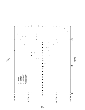
Figure 1: Phase shifts for the pure Coulomb potential at $E_{\rm lab}=1,10,100,300\,$MeV as a function of the matching radius $R$.

The only remaining difficulty is the determination of the matching radius $R$, because the given solution is wrong as long as (3.28) is not valid. On the other hand, it is not possible to extend $R$ to arbitrarily large values, because the cosine in eq.(3.29) will cause rapid oscillations. Therefore, some test calculations are necessary. First, we put a pure Coulomb potential in our framework. In this particular case, the phase shift defined in eq.(3.23) should be zero and $R$ should allowed to be arbitrarily small (but equal to zero). Nevertheless beyond some radius, the abovementioned oscillations are expected. In Fig.1 we have plotted the phase shift for several lab energies in the ${}^{1}S_{0}$ wave. Second, we took the well known Reid93 [26] potential for proton-proton scattering as $V_{\rm strong}$ and re-did the procedure. In Fig.2 we confer our calculation for different $R$ with the published phase shifts of the Reid93-potential at a fixed energy, $E_{\rm lab}=10\,$MeV. As a third check, we compared an r-space solution for a Fourier transformed one-pion-exchange potential of the Bonn-type [27] (dipole cutoff) and the standard Coulomb potential with the same one-pion-exchange in our framework. The checks showed the expected behavior and it seems to be a good choice to define $R=10\,$fm in all partial waves (which is in accordance with a Fourier transformation of our strong potential as well) as it has been done for the Bonn potential [28]. For $R$ less than 5-7 fm, the strong potential is still present, for $R$ bigger than 15 fm, the oscillations can not be neglected.

3.4 Range expansion

It is of particular interest to consider the scattering lengths and effective range parameters. The effective range expansion takes the form (written here for a genuine partial wave)

$$p\,\cot(\delta)=-\frac{1}{a}+\frac{1}{2}\,r\,p^{2}+v_{2}\,p^{4}+v_{3}\,p^{6}+v_{4}\,p^{8}+{\cal O}(p^{10})~{},$$ (3.32)

with $p$ the nucleon cms momentum, $a$ the scattering length and $r$ the effective range. It has been stressed in ref.[29] that the shape parameters $v_{i}$ are a good testing ground for the range of applicability of the underlying EFT since a fit to say the scattering length and the effective range at NLO leads to predictions for the higher order range parameters $v_{i}$.

We now turn to the proton–proton scattering length. It is well–known that the strong hadronic part $a_{pp}$ can only be separated from the one in the presence of the Coulomb interaction $a_{pp}^{C}$ in a regularization scheme dependent way. For a cut–off field theory employing a sharp cut-off as done here, one expects a relation of the form,

$${1\over a_{pp}(\Lambda)}={1\over a_{pp}^{C}}+\alpha\,\left[F\left(\ln{\Lambda\over m}\right)+{\rm const.}\right]~{}.$$ (3.33)

Some explicit examples for the function in the square brackets in a theory where the pions are integrated out are given in ref.[8] (see also [30]). We refrain from further discussing the explicit cut–off dependence of this relation but will come back to this when we discuss the numerical results. It is also important to stress that within the EFT, only a certain range of cut–off values is allowed and thus the often made statement, that the separation of the hadronic scattering length $a_{pp}$ from $a_{pp}^{C}$ is completely arbitrary, does not hold.

4 Renormalized potential

In this section we collect the explicit formulae for the various pieces of the potential expressed in terms of renormalized quantities. The infinities appearing in the TPE diagrams are treated exactly in the same manner as in ref.[4] and we refrain from repeating these arguments here.

Consider first the one–pion exchange (OPE). Its contribution is given in the standard Yukawa form. More precisely, for the $nn$ and the $pp$ systems, only the neutral pion can be exchanged whereas for the $np$ $T=1$ case, we have a superposition of neutral and charged pion exchanges,

$$V^{(0)}_{{\rm OPE},pp}=V^{(0)}_{{\rm OPE},nn} = -\left({g_{A}\over 2F_{\pi}}\right)^{2}\,\vec{\tau}_{1}\cdot\vec{\tau}_{2}\,\,{\vec{\sigma}_{1}\cdot\vec{q}\,\vec{\sigma}_{2}\cdot\vec{q}\over\vec{q}\,^{2}+M_{\pi^{0}}^{2}}~{},$$ (4.1)

$$V^{(0)}_{{\rm OPE},np} = -\left({g_{A}\over 2F_{\pi}}\right)^{2}\,\vec{\tau}_{1}\cdot\vec{\tau}_{2}\,\vec{\sigma}_{1}\cdot\vec{q}\,\vec{\sigma}_{2}\cdot\vec{q}\,\biggl{(}{2\over\vec{q}\,^{2}+M_{\pi^{+}}^{2}}-{1\over\vec{q}\,^{2}+M_{\pi^{0}}^{2}}\biggr{)}~{},$$ (4.2)

with $\vec{q}=(\vec{p}\,^{\prime}-\vec{p}\,)$ the exchanged momentum in the centre-of-mass system, where $\vec{p}$ and $\vec{p}\,^{\prime}$ denote the cms momentum of the incoming and the outgoing two–nucleon pair, in order. For later comparison, we also give the isospin symmetric one–pion exchange potential, it reads

$$V^{(0)}_{{\rm OPE},{\rm sym}}=-\left({g_{A}\over 2F_{\pi}}\right)^{2}\,\vec{\tau}_{1}\cdot\vec{\tau}_{2}\,{\vec{\sigma}_{1}\cdot\vec{q}\,\vec{\sigma}_{2}\cdot\vec{q}\over\vec{q}\,^{2}+M_{\pi}^{2}}~{},$$ (4.3)

with

$$M_{\pi}=\frac{2}{3}M_{\pi^{+}}+\frac{1}{3}M_{\pi^{0}}=138.03~{}{\rm MeV}~{},$$ (4.4)

the average pion mass. So far, we have expressed the pion–nucleon coupling in terms of the Lagrangian parameters $g_{A}$ and $F_{\pi}$. With the help of the Goldberger–Treiman relation $g_{\pi NN}=g_{A}m_{N}/F_{\pi}$ it is then possible to write down these coupling in a more familiar form. As explained above, we do not need to worry about possible isospin breaking effects in $g_{\pi NN}$. They are not only suppressed by the power counting but also known to be small in the most recent phase shift analysis [14].

Consider now the TPE potential. At NLO, for the case of equal pion masses, we can use eq.(2.12) of ref.[4] with the average pion mass as defined in eq.(4.4). We give this expression here for completeness,

$$V_{2\pi,{\rm sym}} = -\frac{\vec{\tau}_{1}\cdot\vec{\tau}_{2}}{384\pi^{2}F_{\pi}^{4}}\,L(q)\,\biggl{\{}4M_{\pi}^{2}(5g_{A}^{4}-4g_{A}^{2}-1)+q^{2}(23g_{A}^{4}-10g_{A}^{2}-1)+\frac{48g_{A}^{4}M_{\pi}^{4}}{4M_{\pi}^{2}+q^{2}}\biggr{\}}$$ (4.5)

$$-\frac{3g_{A}^{4}}{64\pi^{2}F_{\pi}^{4}}\,L(q)\,\biggl{\{}\vec{\sigma}_{1}\cdot\vec{q}\,\vec{\sigma}_{2}\cdot\vec{q}-q^{2}\,\vec{\sigma}_{1}\cdot\vec{\sigma}_{2}\biggr{\}}+P(\vec{k},\vec{q}\,)~{},$$

$$L(q) = \frac{1}{q}\sqrt{4M_{\pi}^{2}+q^{2}}\,\ln\frac{\sqrt{4M_{\pi}^{2}+q^{2}}+q}{2M_{\pi}}~{},$$ (4.6)

and we have set $q\equiv|\vec{q}\,|$. Obviously, the first term of the NLO isospin symmetric TPEP in eq.(4.5) is isovector while the second one is isoscalar. The polynom $P(\vec{k},\vec{q}\,)$ can be absorbed in the isospin symmetric dimension two four–nucleon contact interactions up to some small finite shifts as discussed in the appendix (in what follows, we will ignore this effect). The pion mass difference in the TPE can be incorporated along the lines outlined in ref.[15]. For completeness, we repeat here the basic steps of that paper and bring the potential in the form appropriate to our discussion. It is most convenient to consider the isoscalar and isovector TPE piece separately,

$$V_{2\pi}=V_{2\pi}^{0}+V_{2\pi}^{1}\,\vec{\tau}_{1}\cdot\vec{\tau}_{2}~{}.$$ (4.7)

For the isoscalar part, we can express the TPE as

$$V_{2\pi}^{0}=\frac{2}{3}V_{2\pi}^{0}(M_{\pi^{+}},M_{\pi^{+}})+\frac{1}{3}V_{2\pi}^{0}(M_{\pi^{0}},M_{\pi^{0}})~{},$$ (4.8)

where the arguments refer to the masses of the two exchanged pions. We remark that due to charge conservation, only similar pions can be exchanged in this case. This explicit form is used in the numerical evaluation with $V_{2\pi}^{0}$ as given in eq.(4.5). It is also instructive to perform a Taylor expansion of this expression around the average pion mass,

$$\frac{2}{3}V_{2\pi}^{0}(M_{\pi^{+}},M_{\pi^{+}})+\frac{1}{3}V_{2\pi}^{0}(M_{\pi^{0}},M_{\pi^{0}})$$ (4.9)

$$= \frac{2}{3}\biggl{(}V_{2\pi}^{0}(M_{\pi},M_{\pi})+2{\partial V^{0}_{2\pi}\over\partial M_{\pi^{+}}}\biggl{|}_{M_{\pi^{+}}=M_{\pi}}(M_{\pi^{+}}-M_{\pi})+{\cal O}(\alpha^{2})\biggr{)}$$

$$+ \frac{1}{3}\biggl{(}V_{2\pi}^{0}(M_{\pi},M_{\pi})+2{\partial V^{0}_{2\pi}\over\partial M_{\pi^{0}}}\biggl{|}_{M_{\pi^{0}}=M_{\pi}}(M_{\pi^{0}}-M_{\pi})+{\cal O}(\alpha^{2})\biggr{)}$$

$$= V_{2\pi}^{0}(M_{\pi},M_{\pi})+\frac{4}{3}{\partial V^{0}_{2\pi}\over\partial M_{\pi^{+}}}\biggl{|}_{M_{\pi^{+}}=M_{\pi}}\frac{1}{3}(M_{\pi^{+}}-M_{\pi^{0}})+\frac{2}{3}{\partial V^{0}_{2\pi}\over\partial M_{\pi^{0}}}\biggl{|}_{M_{\pi^{0}}=M_{\pi}}\biggl{(}-\frac{2}{3}\biggr{)}(M_{\pi^{+}}-M_{\pi^{0}})+{\cal O}(\alpha^{2})$$

$$= V_{2\pi}^{0}(M_{\pi},M_{\pi})+{\cal O}(\alpha^{2})~{},$$

i.e. to order ${\cal O}(\alpha)$ there is no isospin breaking in the isoscalar TPE. For the isovector TPE, we have the general structure

$$V_{2\pi}^{1} = \tau_{1}^{3}\,\tau_{2}^{3}\,V_{2\pi}^{1}(M_{\pi^{+}},M_{\pi^{+}})+(\vec{\tau}_{1}\cdot\vec{\tau}_{2}-\tau_{1}^{3}\,\tau_{2}^{3})\,V_{2\pi}^{1}(M_{\pi^{+}},M_{\pi^{0}})$$ (4.12)

$$= \left\{\begin{array}[]{ll}V_{2\pi}^{1}(M_{\pi^{+}},M_{\pi^{+}})&{\rm for}~{}~{}pp~{}~{}{\rm and}~{}~{}nn\\ 2V_{2\pi}^{1}(M_{\pi^{+}},M_{\pi^{0}})-V_{2\pi}^{1}(M_{\pi^{+}},M_{\pi^{+}})&{\rm for}~{}~{}np,T=1\end{array}\right.\quad.$$

Clearly, for the $pp$ (and the $nn$) system, we have to use the charged pion mass. In case of $np$, we use for the numerical evaluation the expression in eq.(4.12). If one again considers the pion mass difference as a small effect and Taylor expands around its average value, one finds that to order $\alpha$ one has to use the neutral pion mass in $V_{2\pi}^{1}$ for the $T=1$ $np$ system.

The $\pi\gamma$ exchange diagrams have already been obtained in ref.[14] and we use the results obtained in that paper omitting all computational details here (although it should be stressed that the treatment of the divergent loop integrals has to be considered approximative, however, for the accuracy of our calculation it is sufficient). Due to isospin only charged pion exchange can contribute to the $\pi\gamma$ potential $V_{\pi\gamma}$ and thus it only affects the $np$ system. The potential has the form

$$V_{\pi\gamma}(\vec{q}\,) = -{g_{A}^{2}\over 4F_{\pi}^{2}M_{\pi^{+}}^{2}}\,(\vec{\tau}_{1}\cdot\vec{\tau}_{2}-\tau_{1}^{3}\,\tau_{2}^{3})\,\vec{\sigma}_{1}\cdot\vec{q}\,\vec{\sigma}_{2}\cdot\vec{q}\,\,V_{\pi\gamma}(\beta)~{},$$

$$V_{\pi\gamma}(\beta) = {\alpha\over\pi}\biggl{[}-{(1-\beta^{2})^{2}\over 2\beta^{4}(1+\beta^{2})}\ln(1+\beta^{2})+{1\over 2\beta^{2}}-{2\bar{\gamma}\over 1+\beta^{2}}\biggr{]}~{}.$$ (4.13)

Here, $\beta=|\vec{q}\,|/M_{\pi^{+}}$ and $\bar{\gamma}$ is a regularization scheme dependent constant. Consistent with the renormalization procedure adopted in ref.[4] (no finite renormalization), we set $\bar{\gamma}=0$ and the expression for the potential simplifies accordingly. The analytical form of $V_{\pi\gamma}$ is similar to the one of the OPEP but it differs in strength by the factor $\alpha/\pi\simeq 1/400$. Due to this inherent smallness, one only expects it to have some influence on the S–wave scattering length.

Finally, we consider the contact interactions. In the isospin limit and at leading order (i.e. with no derivatives), we have two independent contact interactions and seven at NLO (two derivatives). Particular linear combinations of these terms can be projected onto the appropriate partial waves, specifically the two S–waves (${}^{1}S_{0},^{3}S_{1}$), the four P–waves (${}^{1}P_{0},^{3}P_{j}$) and the mixing parameter $\epsilon_{1}$ of the coupled ${}^{3}S_{1}-^{3}D_{1}$ system (for $T=0$). For the two nucleon systems with $T=1$, one has of course only the singlet S–wave and the three triplet P–waves. In case of CIB and CSB, each of the next–to–leading order S–wave contact terms consists actually of three different contributions, namely the isospin symmetric part $C_{\rm sym}$ (with two derivatives) as defined in ref.[4], the CIB part $\sim\tau_{1}^{3}\,\tau_{2}^{3}$ and, the CSB part $\sim(\tau_{1}^{3}+\tau_{2}^{3})$ . Four the P–waves, we only have the two–derivative isospin symmetric contact terms since the equivalent CIB and CSB contact interactions only appear at two orders higher. Therefore, we concentrate on the S–waves. The evaluation of these interactions in the different isospin channels leads to the following contribution to the various NN potentials

$$C_{pp} = C_{\rm sym}+C_{\rm CIB}+C_{\rm CSB}~{},$$ (4.14)

$$C_{nn} = C_{\rm sym}+C_{\rm CIB}-C_{\rm CSB}~{},$$ (4.15)

$$C_{np} = C_{\rm sym}-C_{\rm CIB}~{}.$$ (4.16)

As long as only the $pp$ and the $np$ phase shift are used to pin down the parameters accompanying these contact interactions, one can extract from the contact interactions

$$C_{pp}-C_{np} = 2C_{\rm CIB}+C_{\rm CSB}~{},$$

$$C_{pp}+C_{np} = 2C_{\rm sym}+C_{\rm CSB}~{}.$$ (4.17)

Only if one has access to a third observable, a separation of these three different contributions is possible. In the ${}^{1}S_{0}$ channel, the $nn$ scattering length and the effective range come into play. These can be measured by various methods (as discussed below) and for that particular partial wave, we can then separate the isospin symmetric, CIB and CSB contributions to the coupling constant $C$ via

$$C_{\rm CSB}=\frac{1}{2}(C_{pp}-C_{nn})~{},$$ (4.18)

$$C_{\rm CIB}=\frac{1}{2}(C_{pp}-C_{np}-C_{\rm CSB})~{}.$$ (4.19)

This finishes our formal discussion and we now turn to the results.

5 Results and discussion

5.1 Fitting procedure

First, we must fix the parameters. Throughout, we work with $g_{A}=1.26$, $m_{p}=938.27\,$MeV, $m_{n}=939.57\,$MeV, $M_{\pi^{0}}=134.98\,$MeV and $M_{\pi^{+}}=139.57\,$MeV. Next, we describe the fitting procedure to pin down the LECs. We proceed along the same lines as detailed in [4]. We perform two types of fits. The global ones are obtained by fitting to the phase shifts of the Nijmegen partial wave analysis for the $np$ and the $pp$ case [26]. More precisely, the isospin–symmetric LO and NLO LECs are determined from a best fit to the S–wave ${}^{1}S_{0}$ and the three triplet P–waves ${}^{3}P_{0,1,2}$ at laboratory energies of 1, 5, 10, 25 and 50 MeV and the N${\rm LO}\!\!\!\!/$  LECs entirely from the singlet S–wave (for $np$ and $pp$). Alternatively, for the S–wave we also use the scattering lengths to determine the isospin breaking LECs. This fit is marked by a “$\star$”. We work with a sharp momentum–space regulator $\Lambda$ in the LS equation. The errors for the partial waves are taken from ref. [26]. For a certain range of $\Lambda$, the $\chi^{2}$ distribution is shallow as expected in any cut–off EFT. Here, we are only interested in the cut–off range which allows to simultaneously fit the $np$ and the $pp$ systems. This is the case for the range $300~{}{\rm MeV}\leq\Lambda\leq 500$ MeV. The upper limit in this range is given by the fit to the $pp$ partial waves. We remark that as a check we have reproduced the results of ref.[4] for the $np$ case (for the parameters and cut–offs used there). The corresponding values for the LECs are collected in table 1 for $\Lambda=500\,$MeV and the cut–off dependence of the LO and NLO S–wave LECs is given in table 2.

	${}^{1}S_{0}$	${}^{1}S_{0}~{}\star$	${}^{3}P_{0}$	${}^{3}P_{1}$	${}^{3}P_{2}$
$C^{\rm LO}_{np}$ [104 GeV-2]	$-$0.133	$-$0.093	$--$	$--$	$--$
$C^{\rm NLO}_{np}$ [104 GeV-4]	1.822	2.125	1.335	$-$0.394	0.191
$C^{\rm LO}_{pp}$ [104 GeV-2]	$-$0.129	$-$0.086	$--$	$--$	$--$
$C^{\rm NLO}_{pp}$ [104 GeV-4]	1.822	2.125	1.335	$-$0.394	0.191

Table 1: Values of the LECs for in the various partial waves for a sharp cut–off $\Lambda=500\,$MeV.

$\Lambda$ [MeV]	300	400	500
$C^{\rm LO}_{np}$ [104 GeV-2]	$-$0.1550	$-$0.1545	$-$0.1331
$C^{\rm NLO}_{np}$ [104 GeV-4]	1.613	1.621	1.822
$C^{\rm LO}_{pp}$ [104 GeV-2]	$-$0.1537	$-$0.1532	$-$0.1290
$C^{\rm NLO}_{pp}$ [104 GeV-4]	1.613	1.621	1.822

Table 2: Values of the LECs for in the ${}^{1}S_{0}$ partial waves as a function of the sharp cut–off.

5.2 Phase shifts

Having determined the LECs, we can now predict the S– and P–waves for energies larger than 50 MeV and all other partial waves are parameter free predictions. To be specific, we employ the cut–off $\Lambda=500\,$ MeV. In Fig.3, we show the ${}^{1}S_{0}$ partial wave for energies up to 200 MeV. As noted in ref. [4], for an improved description of this partial wave up to $E_{\rm lab}=300$ MeV, one has to go to NNLO. The triplet P–waves are collected in Fig.4. As already pointed out in [4], the pion mass difference plays an important role in ${}^{3}P_{0}$ for which we get a good description up to $E_{\rm lab}=200\,$MeV. The good description of the ${}^{3}P_{1}$ phase up to the inelastic threshold can be traced back to the dominance of the OPE. The insufficient description of the ${}^{3}P_{2}$ wave was already be observed in [4] and can be cured to some extend at N²LO. Some higher partial waves $(^{1}D_{2},^{3}F_{2},^{3}F_{3},^{1}G_{4})$, which are free of tunable parameters at NLO, are shown in Fig.5. Depending on the partial wave, we find satisfactory description of these waves up to 150 MeV. This holds in particular for the mixing parameter $\epsilon_{2}$ not shown in the figure. These results can be improved by going to NNLO, but for our purpose the accuracy achieved for lab energies up to 150$\ldots$200 MeV is sufficient. In particular, it allows to study CIB and CSB which is most pronounced in the threshold region.

5.3 Charge independence breaking

In the absence of $nn$ data, we define

$$X_{\rm CIB}=X_{pp}-X_{np}~{},\quad X=\{\delta,a,r,v_{1},v_{2},v_{3}\}~{},$$ (5.1)

for the pertinent phase shift, scattering length and range parameters (in a given partial wave). We show first the energy dependence of $\delta_{\rm CIB}$ in the various partial waves, in comparison to the Nijmegen PSA and the most recent results obtained from the CD-Bonn potential. The S– and P–waves are collected in Figs.6 and 7, respectively. In the S–wave, our prediction for energies above 50 MeV shows an interesting difference to the result of the CD-Bonn potential (filled squares in fig.6). In that approach a phenomenological term had to be added to describe correctly the CIB in the scattering lengths, this affects in particular the CIB difference above $E_{\rm lab}=50\,$MeV as depicted by the open squares. The prediction by ignoring this additional term, whose explicit structure is not spelled out in ref.[7], agrees with our full N${\rm LO}\!\!\!\!/$ result. For ${}^{3}P_{1,2}$, our predictions based on the Nijmegen PSA are distinctively different from the CD-Bonn results, however, these phase differences are in both cases of very small magnitude. The CIB in the higher partial waves is shown in Fig.8, only in ${}^{3}F_{3}$ one finds some difference between our prediction and the one obtained using the CD-Bonn potential.

We now turn to the scattering lengths and range parameters. To be specific, we consider the ${}^{1}S_{0}$ partial wave. The $np$ and $pp$ scattering lengths as a function of the cut–off $\Lambda$ are given in table 3. While the result for $a_{np}$ is, of course, independent of the cut–off (within an accuracy of about 0.3%), the $pp$ scattering length varies due to the subtraction ambiguity discussed in section 3.4. It is, however, gratifying to see that within the range of allowed cut–offs, this variation is modest, i.e. $|\delta a_{pp}/a_{pp}|\simeq 0.6~{}{\rm fm}/17~{}{\rm fm}\simeq 3\%.$ Consequently, we get

$$a_{\rm CIB}=6.14\ldots 6.75~{}{\rm fm}~{},$$ (5.2)

for $\Lambda=300\ldots 500\,$MeV.

$\Lambda$ [MeV]	300	400	500
$a_{np}$ [fm]	$-$23.65	$-$23.67	$-$23.71
$a_{pp}$ [fm]	$-$17.51	$-$17.53	$-$16.96

Table 3: $np$ and $pp$ scattering lengths in ${}^{1}S_{0}$ partial wave for the range of cut–off parameters discussed in the text.

To further dissect the physics underlying CIB, we list in table 4 the various contributions to the CIB in the scattering length and effective ranges due to the neutron–proton mass difference ($\Delta m_{N}$), the pion–mass difference ($\Delta M_{\pi}$) in OPE and TPE, from $\pi\gamma$ graphs and due to the contact interactions. These contributions have been obtained in the following manner: The total potential is a sum of different terms and to assess the importance of one particular mechanism, we simply switch that term off and obtain its contribution as the difference between the full result and the one in the absence of that term. Due to the inherent non–linearity of the problem (iteration of the potential, pseudo–boundstate close to threshold) the sum of the individual contributions does not give the full result. In the literature one can find a set of prescriptions to rescale these contributions based on an expansion in the inverse of the scattering length. We do not follow these schemes but stick to the prescription just outlined. As expected, the pion mass difference is a very important effect, but is alone insufficient to account for the CIB in the scattering lengths. The TPE contribution deserves some discussion. It has already been worked out in ref.[15], where a similar result with an opposite sign was found. There are several reasons for that disagreement. First of all, the authors of ref.[15] performed all calculations in configuration space whereas we are working in momentum space. Several zero range terms arising by Fourier transformation of the non–polynomial part of eq.(4.5) have not been taken into account in ref.[15]. Secondly, we are using a sharp momentum cut–off whereas some smooth local coordinate space cut–off has been applied in ref.[15]. Finally, the charge independent part of the potential was chosen in [15] to be the one of the Argonne AV18 potential. In this sense, our description is more consistent and is entirely based on the potential derived within chiral EFT. Therefore, a direct comparison with the numerical results of [15] should not be made. We find the same ordering in the importance of the three types of diagrams, box larger than triangle larger than football. However, there is also a strong cut–off dependence, e.g. the box diagram contribution to $a_{\rm CIB}$ changes form -1.6 fm to -1.1 fm as $\Lambda$ varies from 500 to 300 MeV. Such a strong cut–off dependence has, in fact, to be expected, since neither the contribution to CIB of the complete CIP TPE nor of its non–polynomial part, shown in table 4, correspond to any observable quantity. Only the complete CIB contribution to phase shifts can be measured experimentally. The $\pi\gamma$ contribution agrees with the findings in ref.[14]. Finally, we would like to stress the rather sizeable contribution of the contact interactions to $a_{\rm CIB}$, which deserve some study within models of CIB.

	$\Delta m_{N}$	$\Delta M_{\pi}$ OPE	$\Delta M_{\pi}$ TPE	$\pi\gamma$	contact
$a$ [fm]	0.1284	2.9173	$-$1.1376	$-$0.4203	4.5083
$r$ [fm]	$-$0.0019	$-$0.0804	0.0135	0.0066	$-$0.0739
$v_{1}$ [fm3]	$-$0.0018	$-$0.2684	0.0083	0.0143	$-$0.0589
$v_{2}$ [fm5]	$-$0.0120	$-$2.2246	0.0541	0.0893	$-$0.4249
$v_{3}$ [fm7]	$-$0.0719	$-$17.800	0.2830	0.5606	$-$2.5355

Table 4: Various contributions to CIB in the ${}^{1}S_{0}$ partial wave for a sharp cut–off $\Lambda=500$ MeV as explained in the text.

5.4 The $nn$ system and charge symmetry breaking

To discuss charge symmetry breaking, one has to know the $nn$ scattering length. With the “standard value” of $a_{nn}=-18.9\pm 0.4\,$fm one obtains the value given in eq.(1.3). However, a recent measurement performed at Bonn University using $nd$ breakup combined with exact solutions of the three–body problem gives a sizeably lower value, $a_{nn}=-16.4\pm 0.4\,$fm . For the central value of the Bonn result, we get

$$a_{\rm CSB}=-0.9~{}{\rm fm}~{},$$ (5.3)

which is smaller in size than the value of eq.(1.3) and of opposite sign. As discussed before, we can not predict this scattering length due to the presence of a four–nucleon LEC but rather use the value of $a_{nn}$ as input to predict the $nn$ ${}^{1}S_{0}$ phase shift shown in Fig.9 in comparison to the $np$ and $pp$ phases. Note also that CSB dies out much faster than CIB, at $E_{\rm lab}=25\,$MeV the two $nn$ curves are identical. It is also interesting to investigate the origin of CSB in the EFT. At NLO, there are two effects, namely the nucleon mass difference and the short–distance physics encoded in the leading order CSB four–nucleon interaction. While in the case based on eq.(1.3), the nucleon mass difference effect (0.33 fm) and the contact term (1.27 fm) go in the same direction, for a scattering length as in eq.(5.3), the short distance physics encoded in the contact interaction (-1.21 fm) has to overcome the positive contribution from the nucleon mass difference (0.29 fm). This becomes more transparent if we work out the LECs as defined in eqs.(4.18,4.19) at leading order. Using the standard value for $a_{nn}$, we have (in units of $10^{4}$ GeV^-2),

$$C_{\rm CIB}=0.0026~{},\quad C_{\rm CSB}=0.0012~{},$$ (5.4)

whereas the value of the scattering length from the Bonn measurement gives

$$C_{\rm CIB}=0.0036~{},\quad C_{\rm CSB}=-0.0008~{}.$$ (5.5)

We remark that the importance of the contact term contributions to CSB is in agreement with findings in the CD–Bonn potential, where CSB is largely driven by TPE with non–nucleonic intermediate states. Such contributions are subsumed in the contact interactions of our approach. It is also interesting to compare these NLO results with ones obtained in the KSW scheme [11], cf. Fig.10. As it has already been found in the isospin symmetric calculations, both schemes give similar results in the low energy region but the KSW scheme can not be applied systematically for momenta larger than the pion mass.

6 Summary

In this paper, we have calculated charge independence and charge symmetry breaking in the two–nucleon system based on a chiral effective field theory. This naturally extends the results for the $np$ system presented in refs.[3, 4]. The results of this investigation can be summarized as follows:

1. Based on a modified Weinberg power counting (as explained in ref.[3]), we have systematically included strong and electromagnetic isospin violation in a chiral two–nucleon potential at NLO. Strong isospin violation is due to the light quark mass difference and can easily be incorporated by means of an external scalar source. The electromagnetic effects due to hard photons are represented by local contact interactions. Soft photons appear in loop diagrams and also generate the long–range Coulomb potential. The corresponding classification scheme for the various contributions to CIB and CSB based on the extended power counting at ${\rm LO}\!\!\!\!/$ and N${\rm LO}\!\!\!\!/$ is given in section 3.2.

2. The resulting potential consists of two distinct pieces, the strong (nuclear) potential including isospin violating effects and the Coulomb potential. The nuclear potential consists of one– and two–pion exchange graphs (with different pion and nucleon masses), $\pi\gamma$ exchange diagrams and a set of local four–nucleon operators (some of which are isospin symmetric, some depend on the quark charges and some on the quark mass difference). Since the nuclear effective potential is naturally formulated in momentum space, we use the matching procedure developed in ref.[25] to incorporate the correct asymptotical Coulomb states. The necessary regularization of the potential is performed on the level of the Lippmann–Schwinger equation, using a sharp momentum space cut–off $\Lambda$.

3. The low–energy constants accompanying the contact interactions and the cut–off $\Lambda$ are determined by a simultaneous best fit to the S– and P–waves of the Nijmegen phase shift analysis in the $np$ and the $pp$ systems for laboratory energies below 50 MeV. This allows to predict these partial waves at higher energies and all higher partial waves. Most physical observables come out independent of the cut–off for $\Lambda$ between 300 and 500 MeV. The upper limit on this range is determined by the $pp$ interactions. The resulting phase shifts are shown in figs.3-5, and the CIB phases $\delta_{\rm CIB}=\delta_{pp}-\delta_{np}$ in figs.6-8, in comparison to the outcome of the Nijmegen PSA and recent results based on the CD–Bonn potential [7].

4. We have studied in detail the range expansion for the $np$ and the $pp$ system. For the range of cut–offs, the $pp$ scattering length varies modestly with $\Lambda$ due to the scheme–dependent separation of the nuclear and the Coulomb part, $|\delta a_{pp}/a_{pp}|\simeq 0.6~{}{\rm fm}/17~{}{\rm fm}\simeq 3\%$. We have dissected the various contributions to CIB in the scattering length, reconfirming the importance of the pion mass difference in the OPE. The TPE contribution is smaller in size but of opposite sign, and also strongly cut–off dependent.

5. We have also studied the $nn$ system, performing effective range fits based on the “standard” value for $a_{nn}=-18.9\,$fm and using the most recent result from deuteron break-up, $a_{nn}=-16.4\,$fm [9]. This leads to rather different physics underlying charge symmetry breaking, as discussed in section 5.4.

We have shown that charge independence and charge symmetry breaking can be systematically studied in an effective field theory based on a modified Weinberg power counting. In the future, it would be of interest to also study the effects of two–pion exchange diagrams with the inclusion of explicit delta degrees of freedom to further dissect the physics underlying CIB and CSB. In addition, one should also include vacuum polarisation and magnetic moment corrections to the Coulomb potential if one wants to achieve the same precision as in the so–called modern potentials. Work along such lines is in progress.

Appendix A Closer look at the two–pion exchange potential

In this appendix we discuss in more detail the CIB contributions from the TPEP. In fact, we will show that one generates some polynomial pieces at N${\rm LO}\!\!\!\!/$  which lead to finite shifts in some LECs. However, the effect of these shifts will turn out to be numerically very small. Nevertheless, when improving the accuracy of our potential, such effects have to be taken into account.

In the isospin symmetric case, we can write the NLO TPEP $V^{(2)}_{2\pi,{\rm 1-loop}}$in the form, see also eq.(4.5),

$$V^{(2)}_{2\pi,{\rm 1-loop}}=V^{\rm TPEP}_{\rm non-polynom}+(S_{1}+S_{2}\,q^{2})\,(\vec{\tau}_{1}\cdot\vec{\tau}_{2})+S_{3}\,\biggl{[}(\vec{\sigma}_{1}\cdot\vec{q}\,)\,(\vec{\sigma}_{2}\cdot\vec{q}\,)-(\vec{\sigma}_{1}\cdot\vec{\sigma}_{2})\,q^{2}\biggr{]}~{},$$ (A.1)

with

$$S_{1} = \frac{1}{384\pi^{2}F_{\pi}^{4}}\biggl{\{}-18M_{\pi}^{2}(5g_{A}^{4}-2g_{A}^{2})\ln\frac{M_{\pi}}{\varepsilon}-M_{\pi}^{2}(61g_{A}^{4}-14g_{A}^{2}+4)$$ (A.2)

$$\qquad\qquad\qquad\qquad\qquad\qquad+18M_{\pi}^{2}(5g_{A}^{4}-2g_{A}^{2})J_{0}-3(3g_{A}^{4}-2g_{A}^{2})J_{2}\biggr{\}}~{},$$

$$S_{2} = \frac{1}{384\pi^{2}F_{\pi}^{4}}\biggl{\{}(-23g_{A}^{4}+10g_{A}^{2}+1)\ln\frac{M_{\pi}}{\varepsilon}-{1\over 2}(13g_{A}^{4}+2g_{A}^{2})+(23g_{A}^{4}-10g_{A}^{2}-1)J_{0}\biggr{\}},$$ (A.3)

$$S_{3} = -\frac{3g_{A}^{4}}{64\pi^{2}F_{\pi}^{4}}\biggl{\{}\ln\frac{M_{\pi}}{\varepsilon}+\frac{1}{3}-J_{0}\biggr{\}}~{},$$ (A.4)

in terms of the divergent loop functions $J_{0,2}$, the IR regulator $\varepsilon$ (for details, see ref.[4]) and the non–polynomial part is given in eq.(4.5). From here on, we concentrate on the polynomial terms, which have the genuine structure

$$V^{\rm TPEP}_{\rm polynom}=V^{0}_{\rm polynom}+V^{1}_{\rm polynom}\,\vec{\tau}_{1}\cdot\vec{\tau}_{2}~{}.$$ (A.5)

Again, the pion mass difference $\Delta M_{\pi}^{2}\sim\alpha$ will lead to CIB. Following the same arguments as used in section 4, up to corrections of order $\alpha^{2}$, one uses the various pion masses in the polynomial pieces as explained for the non–polynomial ones. To be specific, consider the $T=1$ $np$ case. We denote the corresponding LECs by $C_{S},C_{T},C_{i}$. Putting in the appropriate pion masses, one finds for the isovector piece

$$V^{1}_{{\rm polynom},pp,nn}-V^{1}_{{\rm polynom},np} = V^{1}_{\rm polynom}(M_{\pi^{\pm}})-V^{1}_{\rm polynom}(M_{\pi^{0}})$$ (A.6)

$$= (A+B\,q^{2})\,\vec{\tau}_{1}\cdot\vec{\tau}_{2}~{}.$$

The term $\sim A$ leads to a relative shift between $C_{pp}^{\rm LO}$, $C_{nn}^{\rm LO}$, and $C_{np}^{\rm LO}$ in the ${}^{1}S_{0}$ wave. However, we do not need to know the precise value of this shift (and thus of the constant $A$) since these LECs are any way fitted independently. To the contrary, one has to know the value of $B$,

$$B={1\over 384\pi^{2}F_{\pi}^{4}}\biggl{(}-23g_{A}^{4}+10g_{A}^{2}+1\biggr{)}\,\ln\frac{M_{\pi^{\pm}}}{M_{\pi^{0}}}=-4.98~{}{\rm GeV}^{-4}~{}.$$ (A.7)

This leads to finite shifts in the NLO LECs,

$$\Delta C_{{}^{s}L_{j}}^{\rm NLO}=C_{pp,nn,^{s}L_{j}}^{\rm NLO}-C_{np,^{s}L_{j}}^{\rm NLO}~{},$$ (A.8)

in the usual spectroscopic notation. We find

$$\Delta C_{{}^{1}S_{0}}^{\rm NLO}=4\pi B~{},\quad\Delta C_{{}^{3}P_{j}}^{\rm NLO}=-\frac{8\pi}{3}B~{},$$ (A.9)

so that

$$C_{pp,nn,^{1}S_{0}}^{\rm NLO}=\biggl{(}C_{np,^{1}S_{0}}^{\rm NLO}-0.0063\biggr{)}\cdot 10^{4}\,{\rm GeV}^{-4}~{},$$

$$C_{pp,nn,^{3}P_{j}}^{\rm NLO}=\biggl{(}C_{np,^{3}P_{j}}^{\rm NLO}+0.0042\biggr{)}\cdot 10^{4}\,{\rm GeV}^{-4}~{}.$$ (A.10)

The effect of these shifts is numerically very small, as demonstrated for the ${}^{1}S_{0}$, ${}^{3}P_{0}$ and ${}^{3}P_{1}$ waves in fig.11.

Figures

 

Figure 2: ${}^{1}S_{0}$ phase shift for Reid93 plus Coulomb potential at $E_{\rm lab}=10\,$MeV (solid line) for varying matching radius (dashed line).

Figure 3: ${}^{1}S_{0}$ phase shifts for the $np$ and $pp$ systems (solid and dashed line, respectively) im comparison to the Nijmegen PSA, filled circles: $np$, open circles: $pp$.

Figure 4: P–wave phase shifts for the $np$ and $pp$ systems im comparison to the Nijmegen PSA. For notations, see Fig.3.

Figure 5: Higher partial waves for the $np$ and $pp$ systems in comparison to the Nijmegen PSA. For notations, see Fig.3.

Figure 6: CIB ${}^{1}S_{0}$ phase shift (solid line) im comparison to the Nijmegen PSA (dashed line) and the CD-Bonn potential (filled and open squares, as explained in the text).

Figure 7: CIB P–wave phase shifts in comparison to the Nijmegen PSA and the CD-Bonn potential. For notations, see Fig.6.

Figure 8: CIB phase shifts in the higher partial waves in comparison to the Nijmegen PSA and the CB-Bonn potential. For notations, see Fig.6.

Figure 9: Range fit for the $nn$ ${}^{1}S_{0}$ phase shift based on different scattering lengths $(a_{nn}=-18.9\,$fm: long-dashed line, $a_{nn}=-16.4\,$fm: short-dashed line) in comparison to the $np$ and $pp$ phases. For further notations, see Fig.3.

Figure 10: Range fit for the $nn$ and $np$ ${}^{1}S_{0}$ phase shifts. The long-dashed and long-short-dashed lines refer to the $np$ and $nn$ results at NLO in the KSW counting [11]. The results of the present approach are: $np$ solid line, $nn$ with $a_{nn}=-18.9,-16.4\,$fm: dotted and and short-dashed line, respectively. The filled circles are the Nijmegen PSA values.

Figure 11: Effect of the polynomial TPEP shifts on the ${}^{1}S_{0}$, ${}^{3}P_{0}$, ${}^{3}P_{1}$ waves as discussed in the appendix. The (solid) dashed lines correspond to (not) incorporating the finite shifts as given in eq.(A.10).

References

- [1] S. Weinberg, Nucl. Phys. B363 (1991) 3.
- [2] D.B. Kaplan, M.J. Savage and M.B. Wise, Nucl. Phys. B534 (1998) 329.
- [3] E. Epelbaoum, W. Glöckle and Ulf-G. Meißner, Nucl. Phys. A637 (1998) 107.
- [4] E. Epelbaum, W. Glöckle and Ulf-G. Meißner, Nucl. Phys. A671 (2000) 295.
- [5] G.A. Miller, B.M.K. Nefkens and I. Slaus, Phys. Rep. 194 (1990) 1.
- [6] S.A. Coon, nucl-th/9903033.
- [7] R. Machleidt, nucl-th/0006014.
- [8] X. Kong and F. Ravndal, Nucl. Phys. A665 (2000) 137.
- [9] V. Huhn et al., Phys. Rev. Lett. 85 (2000) 1190.
- [10] J.L. Friar and S.A. Coon, Phys. Rev. C53 (1996) 588.
- [11] E. Epelbaum and Ulf-G. Meißner, Phys. Lett. B461 (1999) 287.
- [12] G.Q. Li and R. Machleidt, Phys. Rev. C58 (1998) 259.
- [13] U. van Kolck, Phys. Rev. C49 (1994) 2932.
- [14] U. van Kolck et al., Phys. Rev. Lett. 80 (1998) 4386.
- [15] J. Friar and U. van Kolck, Phys. Rev. C60 (1999) 034006.
- [16] V. Bernard, N. Kaiser and Ulf-G. Meißner, Int. J. Mod. Phys. E4 (1995) 193.
- [17] G. Ecker, J. Gasser, A. Pich and E. de Rafael, Nucl. Phys. B321 (1989) 311.
- [18] R. Urech, Nucl. Phys. B433 (1995) 234.
- [19] H. Neufeld and H. Rupertsberger, Z. Phys. C68 (195) 91.
-
[20]
Ulf-G. Meißner, G. Müller and S. Steininger,
Phys. Lett. B406 (1997) 154,
(E) ibid B407 (1997) 434. - [21] M. Knecht and R. Urech, Nucl. Phys. B519 (1998) 329.
- [22] N. Fettes, Ulf-G. Meißner and S. Steininger, Nucl. Phys. A640 (1998) 199.
- [23] Ulf-G. Meißner and S. Steininger, Phys. Lett. B419 (1998) 403.
- [24] G. Müller and Ulf-G. Meißner, Nucl. Phys. B556 (1999) 265.
- [25] C.M. Vincent, S.C. Phatak, Phys. Rev. C10 (1974) 391.
- [26] V.G.J. Stoks et al., Phys. Rev. C49 (1994) 2950.
- [27] R. Machleidt, K. Holinde, Ch. Elster, Phys. Rep. 149 (1987) 1.
- [28] J. Haidenbauer and K. Holinde, Phys. Rev. C40 (1989) 2465.
- [29] T.D. Cohen and J.M. Hansen, Phys. Rev. C59 (1999) 13.
- [30] B.R. Holstein, Phys. Rev. D60 (1999) 114030.