Hadronic interactions of the $J/\psi$

Abstract

We calculate the cross sections for reactions of the $J/\psi$ with light mesons. We also evaluate its finite temperature spectral function. We investigate separately the role of elastic and inelastic channels and we compare their respective importance. We describe $J/\psi$ absorption channels that have not been considered previously to our knowledge. The relevance of our study to heavy ion collisions is discussed.

I Introduction

The study of relativistic heavy ion collisions offers the tantalizing possibility of observing many-body effects in a strongly interacting system at densities and temperatures far removed from equilibrium. At ultrarelativistic energies, the main focus of the active experimental and theoretical programs is the creation, observation, and interpretation of a new form of matter: the quark-gluon plasma. Its existence is a prediction of QCD, even though some ambiguities concerning the specific nature of an eventual phase transition and its experimental signatures [1] still remain. It is fair to say that the activity generated by this field makes it one of the most exciting areas of contemporary subatomic physics.

The $J/\psi$ meson has been singled-out as a promising candidate to signal deconfinement. Indeed, the presence of a high temperature quark-gluon plasma would screen the $c\bar{c}$ interaction [2] or ionize the quarkonium state [3], leading to a suppression of the $J/\psi$ in events where the plasma is produced in comparison with events where it is not. While the suppression of $J/\psi$ (and $\psi^{\prime}$) in p-A and in heavy ion collisions involving medium-mass projectiles at 200A GeV [4] can be explained by absorption models without plasma assumptions [5, 6], the subsequent Pb + Pb data has led to analyses involving plasma formation [7]. However, the plasma interpretation of this “anomalous” $J/\psi$ absorption observed with the Pb projectile needs the introduction of model-dependent assumptions. Furthermore, alternative explanations which rest purely on hadronic grounds are starting to appear [8, 9]. Any model of $J/\psi$ suppression, whether it includes hadronic “comovers” [5] or not, relies on simple assumptions about the size of the cross sections with nucleons and light hadrons. Unfortunately, up to recently only a few calculations of the interaction cross section of $J/\psi$ with light hadrons could be found in the published literature [10, 11], and the results of those calculations are not in agreement with each other [12].

Our aim in this work is the following. We plan to systematically explore the different channels of interaction of the $J/\psi$ with light hadrons and calculate the corresponding cross sections, in light of recent calculations with an effective hadronic Lagrangian [13, 14]. We shall perform no attempts to find heavy ion data here. However we will try to bring the study of the hadronic interactions of the $J/\psi$ meson closer to the level of sophistication that the lighter vector mesons ($\rho$, $\omega$, and $\phi$) currently enjoy. Consequently, we calculate the spectral function for the charmonium state, in a gas of light mesons at finite temperature. Bear in mind that this does not imply that the $J/\psi$ is thermalized. We view this calculation as a necessary prelude to a more complete understanding of the behavior of the charmonium bound states in hadronic matter at finite temperature and density. Because of the direct decay into muon pairs, the $J/\psi$ spectral function is directly accessible experimentally.

Our paper is organized as follows: in the next section we discuss details of a heavy meson chiral Lagrangian bearing hadronic interactions upon which our quantitative estimates are based. We also describe a slight variant of this model that has been used in phenomenological applications. The dominant channels in this study, both elastic and inelastic, are then considered and the associated cross sections are shown. We introduce new channels, to our knowledge, for $J/\psi$ absorption on mesons. We then proceed to a discussion of the scattering widths induced by the interactions. We will then show the resulting $J/\psi$ spectral function, and explore its temperature and momentum dependence. We summarize and conclude.

II Chiral Lagrangian for light and heavy mesons

We discuss here the basic assumptions and ingredients in our chiral Lagrangian approach for light and heavy pseudoscalar and vector mesons. We shall model the interaction of the charmonium state with lighter mesons through meson exchanges. In order to include charmed mesons, the smallest possible symmetry group that potentially contains the relevant phenomenology is SU(4). However, SU(4) is in fact badly broken by the large mass of the charmed quark. This also can be seen in the poor agreement obtained between the extended mass formula and the experimentally measured masses [15]. We adopt here the following pragmatic viewpoint: we work here with the physical mass eigenstates and the physical mass matrix will represent the relevant breaking of the original symmetry. Furthermore, we compare two calibration methods, (i) the chiral gauge coupling will be uniquely determined from light vector spectroscopy, namely the $\rho$ meson, and (ii) relevant coupling constants are individually chosen by either empirical constraints where they exist or model calculations in the absence of measurement. We feel that it is crucial for this effective approach to be in tune with the largest possible range of phenomenology at the appropriate energy scale.

Description of light and heavy pseudoscalars in a single framework can be obtained using a four-flavor chiral Lagrangian. The basic nonlinear SU(4) $\sigma$ model apart from mass terms is

$${\cal L}_{0} = {-F_{\pi}^{2}\over 8}{\rm Tr}(\partial_{\mu}U\partial^{\mu}U^{{\dagger}}),$$ (1)

$$U = {\rm exp}\left[{2i\phi\over F_{\pi}}\right].$$ (2)

The constant $F_{\pi}\simeq$ 135 MeV and $\phi$ is the pseudoscalar multiplet matrix. Correct normalization leads to

$$\phi = \left(\begin{array}[]{cccc}\frac{\pi^{0}}{\sqrt{2}}+\frac{\eta}{\sqrt{6}}+\frac{\eta_{c}}{\sqrt{12}}&\pi^{+}&K^{+}&\bar{D}^{0}\\ \pi^{-}&-\frac{\pi^{0}}{\sqrt{2}}+\frac{\eta}{\sqrt{6}}+\frac{\eta_{c}}{\sqrt{12}}&K^{0}&D^{-}\\ K^{-}&\bar{K}^{0}&-\eta\sqrt{\frac{2}{3}}+\frac{\eta_{c}}{\sqrt{12}}&D_{s}^{-}\\ D^{0}&D^{+}&D_{s}^{+}&-3\frac{\eta_{c}}{\sqrt{12}}\\ \end{array}\right)\ ,$$ (7)

To introduce vector mesons we make the replacement

$$\partial_{\mu}U \to {\cal D\/}_{\mu}U\equiv\partial_{\mu}U-igA_{\mu}^{L}U+igUA_{\mu}^{R},$$ (8)

and we add kinetic terms

$${\cal L}_{1} = -{1\over 2}{\rm Tr}\left(F_{\mu\nu}^{L}F^{L\,\mu\nu}+F_{\mu\nu}^{R}F^{R\,\mu\nu}\right)+\gamma\,{\rm Tr}\left(F_{\mu\nu}^{L}UF^{R\,\mu\nu}U^{{\dagger}}\right),$$ (9)

where $A_{\mu}^{L}$ and $A_{\mu}^{R}$ are the chiral spin-1 fields and where

$$F_{\mu\nu}^{L} = \partial_{\mu}A_{\nu}^{L}-\partial_{\nu}A_{\mu}^{L}-ig\left[A_{\mu}^{L},A_{\nu}^{L}\right],$$ (10)

$$F_{\mu\nu}^{R} = \partial_{\mu}A_{\nu}^{R}-\partial_{\nu}A_{\mu}^{R}-ig\left[A_{\mu}^{R},A_{\nu}^{R}\right].$$ (11)

Next we add mass terms for the spin-1 fields plus two generalized mass terms

$${\cal L\/}_{2} = -m_{0}^{2}\,{\rm Tr}\left(A_{\mu}^{L}A^{L\,\mu}+A_{\mu}^{R}A^{R\,\mu}\right)+B\,{\rm Tr}\left(A_{\mu}^{L}UA^{R\,\mu}U^{{\dagger}}\right)+C\,{\rm Tr}\left(A_{\mu}^{L}A^{R\,\mu}+A_{\mu}^{R}A^{L\,\mu}\right).$$ (12)

The aim for the present model is to describe the normal parity states, so we must eliminate the axial-vector matrix field $A_{\mu}\equiv A_{\mu}^{L}-A_{\mu}^{R}$. To accomplish this, we follow the ideas presented in Ref. [16] and make a gauge transformation resulting in $A_{\mu}^{\prime}=0$. Equivalently, in the primed gauge, $A_{\mu}^{L\,\prime}=A_{\mu}^{R\,\prime}\equiv\rho_{\mu}$. The vector meson matrix multiplet is

$$\rho_{\mu}\ =\ \left(\begin{array}[]{cccc}\frac{\rho^{0}}{\sqrt{2}}+\frac{\omega}{\sqrt{6}}+\frac{J/\psi}{\sqrt{12}}&\rho^{+}&{K^{*}}^{+}&\bar{{D^{*}}}^{0}\\ \rho^{-}&-\frac{\rho^{0}}{\sqrt{2}}+\frac{\omega}{\sqrt{6}}+\frac{J/\psi}{\sqrt{12}}&{K^{*}}^{0}&{D^{*}}^{-}\\ {K^{*}}^{-}&\bar{{K^{*}}}^{0}&-\omega\sqrt{\frac{2}{3}}+\frac{J/\psi}{\sqrt{12}}&{D^{*}}_{s}^{-}\\ {D^{*}}^{0}&{D^{*}}^{+}&{D^{*}}_{s}^{+}&-3\frac{J/\psi}{\sqrt{12}}\\ \end{array}\right)_{\mu}\ .$$ (17)

The specific choices $U^{1/2}=\xi$, $U^{-1/2}=\xi^{{\dagger}}$ and

$$A_{\mu}^{L} = \xi\rho_{\mu}\xi^{{\dagger}}+{i\over g}\xi\partial_{\mu}\xi^{{\dagger}}$$ (18)

$$A_{\mu}^{R} = \xi^{{\dagger}}\rho_{\mu}\xi+{i\over g}\xi^{{\dagger}}\partial_{\mu}\xi$$ (19)

$$U = \xi\mbox{\boldmath{$1$}}\xi$$ (20)

will “gauge away” the positive-parity states from the model by producing the requisite $A_{\mu}^{\prime}=0$.

Gauging away the axial fields with the above mentioned transformation yields the following Lagrangian (utilizing Hermiticity $\phi$ = $\phi^{{\dagger}}$ and $\rho_{\mu}=\rho_{\mu}^{{\dagger}}$)

$${\cal L}_{0} = 0$$ (21)

$${\cal L}_{1} = \left(\gamma-1\right){\rm Tr}\left[F_{\mu\nu}(\rho)F^{\mu\nu}(\rho)\right],$$ (22)

$${\cal L}_{2} = \left(B+2C-2m_{0}^{2}\right){\rm Tr}\left(\rho_{\mu}\rho^{\mu}\right)+{2i(B-2C-2m_{0}^{2})\over g\,F_{\pi}^{2}}{\rm Tr}\left(\rho_{\mu}\left[\partial^{\mu}\phi,\phi\right]\right)$$ (23)

$$+{4C\over F_{\pi}^{2}}{\rm Tr}(\left[\phi,\rho^{\mu}\right]^{2})-{(B+2C+2m_{0}^{2})\over g^{2}\,F_{\pi}^{2}}{\rm Tr}\left(\partial_{\mu}\phi\partial^{\mu}\phi\right),$$ (24)

where we have defined

$$F_{\mu\nu}(\rho)\equiv\partial_{\mu}\rho_{\nu}-\partial_{\nu}\rho_{\mu}-ig\left[\rho_{\mu},\rho_{\nu}\right].$$ (25)

We notice that under the gauge transformation the original kinetic piece for the pseudoscalars vanishes—it reappears in ${\cal L\/}_{2}$. ${\cal L\/}_{1}$ becomes a kinetic Yang-Mills term for the field $\rho_{\mu}$, while its correct normalization points to $\gamma=$ 3/4. Furthermore, ${\cal L\/}_{2}$ includes the mass terms for the $\rho_{\mu}$ field, kinetic terms for $\phi$, as well, it includes three-point and four-point interaction terms. It is clear that the mass term for $\rho_{\mu}$ spoils local gauge invariance. In order to leave ${\cal L\/}_{0}+{\cal L\/}_{1}+{\cal L\/}_{2}$ chirally and locally gauge invariant, we choose $B+2C-2m_{0}^{2}=0$. Omitting kinetic energy terms, we arrive at the model’s chiral and gauge invariant set of interactions. They are the following

$${\cal L\/}_{\rm\,int} = ig\,{\rm Tr}\left(\rho_{\mu}\left[\partial^{\mu}\phi,\phi\right]\right)-{g^{2}\over 2}{\rm Tr}(\left[\phi,\rho^{\mu}\right]^{2})+ig\,{\rm Tr}\left(\partial_{\mu}\rho_{\nu}\left[\rho^{\mu},\rho^{\nu}\right]\right)+{g^{2}\over 4}{\rm Tr}(\left[\rho^{\mu},\rho^{\nu}\right]^{2})$$ (26)

where, for convenience, we have attached physical significance to the gauge coupling constant through

$${2(B-2C-2m_{0}^{2})\over g\,F_{\pi}^{2}} = {g_{\rho\pi\pi}\over 2}\ =\ g.$$ (27)

Before leaving the formalism we summarize up to this point. An effective chiral Lagrangian of light plus heavy pseudoscalar and vector mesons has been constructed to be fully chirally U(4)$\times$U(4) invariant. In particular, no loose ends are left in the model since the axial fields have been completely gauged away. The result is written in Eq. (24). From here we further impose local gauge invariance and arrive at interaction terms given in Eq. (26). The model has two input parameters: $F_{\pi}$ and $g_{\rho\pi\pi}$. Since we adjust $g_{\rho\pi\pi}$ using the decay rate into pion pairs at the physical rho pole, we implicitly also use $m_{\rho}$. The matrix algebra implied in the above expressions can now be explicitly carried out to obtain Lagrangians involving specific physical fields.

A Chiral Model Predictions

The model is constructed in some sense to pivot off the rho meson since $\rho$ decay into two pions uniquely determines the gauge coupling constant $g$. Taking $\Gamma_{\rho}$ = 151 MeV, and $m_{\rho}$ = 770 MeV, we find $g_{\rho\pi\pi}={\rm 2}g\simeq$ 8.54. Having fixed the single parameter in Eq. (26), we are in position to “predict” widths for meson decays where phase space is open, and we are particularly interested in the strangeness and charm sectors. $K^{*}$’s and $D^{*}$’s are chosen to test the symmetry breaking effects in the extremes. Results for widths are listed in Table I. We find $K^{*}$ widths consistent to within 10% of experiment, and $D^{*}$ widths consistent with other model calculations[17, 18, 19]. We are hesitant to read too much into these numbers, but they begin to suggest that the symmetry breaking effects might largely be accounted for merely by using the physical mass eigenstates.

All coupling strengths are now in principle fixed. We have first evaluated absorption cross sections for reactions involving the $J/\psi$ in the initial state. We list the processes under consideration in Table II. Note that each process can in principle involve several Feynman diagrams and their interference.

For the sake of brevity, we do not show all the cross sections we have evaluated. We shall restrict ourselves here to the most important ones. Our findings first support the notion that the elastic channels are quantitatively small. Apart from the $\omega$ to be discussed later, the largest contribution in this category is shown in Fig. 1, and is $J/\psi+\rho\rightarrow J/\psi+\rho$. By $\sqrt{s}$ = 6 GeV, the cross section has just about risen to 1 mb. This process is modeled by pion exchange and therefore involves vector-vector-pseudoscalar interactions which are not included in the chiral Lagrangian. Instead, the relevant Lagrangian is

$${\cal L} = g\,\epsilon_{\alpha\beta\mu\nu}\,\partial^{\alpha}V^{\beta}\partial^{\mu}V^{\nu}\,\phi\ .$$ (28)

The coupling strength is fixed to match the measured [26] $J/\psi\to\pi\rho$ decay width.

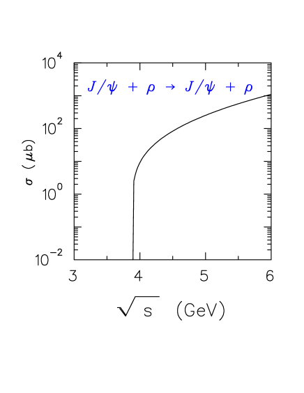
FIG. 1.: Elastic cross section J/$\psi$ + $\rho\rightarrow$ J/$\psi$ + $\rho$.

The elastic process immediately following this one in importance is $J/\psi+\eta\rightarrow J/\psi+\eta$, and the corresponding cross section is only 6 nb at the same value of $\sqrt{s}$. All other elastic processes listed in Table II are at the nb, pb, and even fb level.

We now turn to the most important channels in our study: inelastic reactions. We show in Fig. 2 the isospin averaged total absorption cross section $J/\psi+\pi\rightarrow D^{*}+\bar{D}$ plus $\bar{D}^{*}+D$.

FIG. 2.: Isospin averaged total cross section for J/$\psi$ + $\pi\rightarrow$ $(\bar{\it D\/}$ + D${}^{*})$ + $(\bar{\it D\/}^{*}$ + D).

Next in importance is the reaction $J/\psi+\rho\rightarrow D^{*}\bar{D^{*}}$, this is shown in Fig. 3.

FIG. 3.: Cross section for J/$\psi$ + $\rho\rightarrow$ $\bar{\it D\/}^{*}$ + D^∗.

Note that exothermic reactions are also possible, but they typically settle down to a low cross section value. A representative example is $J/\psi+\rho\rightarrow D+\bar{D}$, and this is shown in Fig. 4.

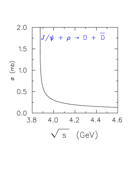
FIG. 4.: Cross section for J/$\psi$ + $\rho\rightarrow$ $\bar{\it D\/}$ + D.

B Phenomenological Model

To compare with other calculations which have used effective Lagrangian methods but have constrained the model differently, we include this subsection. If we retreat somewhat from the symmetry and allow the coupling constants to be separately adjusted to empirical constraints or models we arrive at different predictions. For instance, if we choose the $D^{*}D\pi$ coupling constant to give a width consistent with a relativistic potential model prediction of 46 keV for $D^{*\,\pm}$[20], we find $g_{D^{*}D\pi}$ = 4.4 (whereas, the chiral prediction from the previous subsection used a value 3.02). Vector dominance arguments have been further used to fix couplings like $g_{J/\psi\,DD}$ and $g_{J\/\psi\,D^{*}D^{*}}$ to be 7.7[13, 14]. Again, the chiral prediction used above is 4.93. We stress that the chiral model

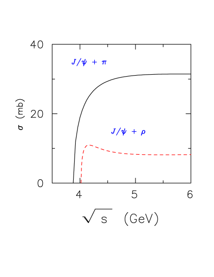
FIG. 5.: Cross sections for pion- and rho meson-induced dissociation of $J/\psi$. The specific channels are the same as Figs. 2 and 3.

calculations are not different from the previous effective Lagrangian methods, practically speaking, the differences are merely methods of calibration [21]. Note however that the calibration method we associated with the “phenomenological model” will lead to K^∗ phenomenology that is off by a factor of two, as seen in Table I.

In Fig. 5 we show pion and rho dissociation of $J/\psi$ in the phenomenological approach. The results are to be compared with the chiral model predictions in Figs. 2 and 3. So in some sense, the different results could be viewed as representative of uncertainties in the present hadronic approaches to $J/\psi$ dynamics. In this work the preference will go to the so-called chiral approach as it generates the hadronic phenomenology contained in Table I which does not contradict experimental measurements.

III Anomalous processes

We include next a section which reports on a couple of processes in the anomalous sector which turn out to give significant cross sections. Based on the observation that $J/\psi\to\eta_{c}+\gamma$ is 1.3% of 87 keV, we use vector dominance to estimate the coupling of $J/\psi$ to $\eta_{c}$ and $\omega$. The Lagrangian we use is again listed in Eq. (28). We find a value $g_{J/\psi\eta_{c}\omega}$ = 9.5 GeV^-1. Using similar reasoning and calculations for $\omega\to\pi^{0}\gamma$, we extract $g_{\omega\rho\pi}$ = 11.6 GeV^-1. Equipped with these couplings, we can compute the cross section for $J/\psi+\pi\to\eta_{c}+\rho$ through $\omega$ exchange. We present it in

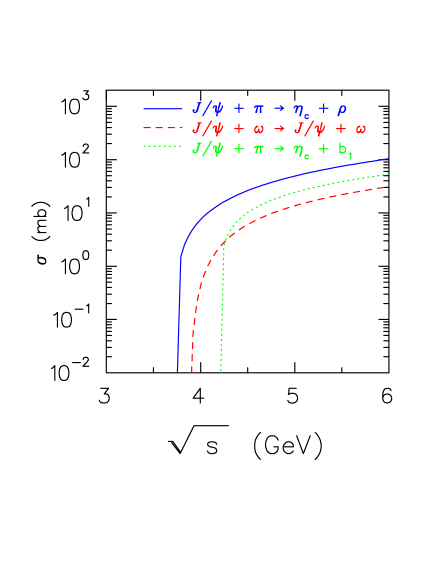
FIG. 6.: Cross sections for $J/\psi$ involving anomalous couplings and the $\eta_{c}$ meson. The specific channels are discussed in the text.

Fig. 6, and remark that it is quite large. Since this calculaton has been done, we have found that Shuryak and Teaney had considered this process previously using a model different from what is done here [22].

Similarly, the cross section for $J/\psi+\pi\to\eta_{c}+b_{1}$ is estimated. The value for the coupling $g_{b_{1}\pi\omega}$ is deduced from the measured decay width of the $b_{1}$ [26]. The cross section is displayed in Fig. 6. Its value is also large. The elastic channel $J/\psi+\omega\to J/\psi+\omega$ proceeding through through $\eta_{c}$ exchange can be considered. It too is included in Fig. 6, and one can also conclude that it is relatively important. We have also calculated several other new reactions which we report on in the next section.

With these cross sections, and the ones associated with all the other processes we have considered, the $J/\psi$ spectral function in a finite temperature gas of mesons can now be calculated. However before moving on to that topic, the important issue of form factors needs to be addressed.

IV Hadronic form factors

The field theory in this work is formulated in a hadronic language and does not deal with fundamental fields but with degrees of freedom that are composite in terms of quark content. It is clear that the exchange of heavy mesons (as the open charm $D$ mesons, for example) leads to an interaction too short-ranged for the interacting particles to be left unmodified [23]. Meson-exchanges are perhaps parameterizations of other phenomena which should be more evident at the parton level. This fact reveals itself in the appearance of hadronic form factors at the interaction vertices of Feynman diagrams. Those can be the source of additional uncertainty in the model. Note that form factor considerations are not restricted to meson exchange models like the one discussed here. For example, they occur also in the flux tube breaking model [24] and the ${{}^{3}}P_{0}$ model [25]. The choice of form factors is guided here by physical arguments, and they are introduced in a way that respects gauge invariance in the electromagnetic sector, and Lorentz symmetry.

A generic form is first chosen to construct $t-$ and $u-$channel hadronic form factors. A candidate that lends itself to practical calculations is the monopole:

$$F(t)={\Lambda^{2}\over\Lambda^{2}+|\,t-m_{\alpha}^{2}|}\ ,$$ (29)

where $m_{\alpha}$ is the mass of the exchanged meson. An advantage of this functional form is that the form factor is normalized to 1 for on-shell particles. Also, even if the kinematics venture into regions of time-like momentum transfer, this choice of form factors remains unitary. Each vertex therefore receives a contribution $F(t)$ or $F(u)$, depending on the appropriate kinematics. The vertices for the tadpole diagrams are determined by replacing its metric tensor structure by a general tensorial expansion constructed from the metric tensor and the available four-vectors. The coefficients of this expansion are then chosen such that the total amplitude is gauge invariant in the electromagnetic sector. The form factors in this work therefore build Feynman amplitudes that are both Lorentz- and gauge-invariant.

Our values for $\Lambda$ stem from elements of hadronic phenomenology which we describe now. We first fix the coupling constant $g_{J/\psi\rho\pi}$ by reproducing the measured width $\Gamma_{J/\psi\to\rho\pi}$. The appropriate vector-vector-pseudoscalar ($VV\phi$) Lagrangian has been shown in Eq. (28). For the determination of $g$ the form factor (Eq. 29) plays no role, by construction. $\Lambda$ is then determined by pushing one of the particles off-shell. Consider the measured [26] radiative decay width $\Gamma_{J/\psi\to\gamma\pi^{0}}$. Using a Vector Meson Dominance (VMD) argument, one may assume that the photon couples to the $\rho$ of the above strong interaction vertex. Then, with $g$ being determined, $\Lambda$ can be obtained from a fit to the radiative decay width. A word of caution is necessary here: the $J/\psi$ also has a $G$-parity violating decay like $J/\psi\to\omega\pi$, so that presumably the photon could also originate from the $\omega$ through VMD. However when compared with $J/\psi\to\rho^{0}\pi^{0}$, the decay into $\omega\pi^{0}$ is suppressed by an order of magnitude so that we can safely ignore it here. In order to reproduce the $J/\psi$ radiative decay width one needs the parameter in Eq. 29 to be $\Lambda$ = 1.25 GeV. This number is satisfying as it does represent a scale that is typically associated with soft hadronic interaction as are commonplace in, for example, the Bonn potential [27].

Another method to pin down hadronic form factors consists of considering $J/\psi$ and open charm photoproduction data and to use their relation with $J/\psi$-nucleon total elastic and inelastic cross sections [28]. Using this argument, a $J/\psi$ + $N$ inelastic cross section can be extracted from the data, and its value is $\approx$0.1 mb at $\sqrt{s}$ = 6 GeV [29]. Below this energy, some doubts have been expressed on the reliability of the cross section extraction through VMD [29]. We estimate the largest contribution to the $J/\psi$-$N$ inelastic cross section to be $J/\psi N\to\Lambda_{c}\bar{D}$. Using the form factor described above and requiring that the inelastic cross section be 0.1 mb at $\sqrt{s}$ = 6 GeV sets $\Lambda$ = 3 GeV. Past this energy value the $J/\psi$-$N$ meson-exchange cross section drops (unlike what is shown in Fig. (5) of Ref. [29]), so that the upper bound set by photoproduction data is not exceeded. With this in mind $\Lambda$ = 2 GeV is set as a conservative upper bound for the remainder of this work, thereby allowing for the contribution of other channels to the $J/\psi-N$ cross section.

Summarizing, a range in $\Lambda$ was estimated for the hadronic form factor introduced in the meson exchange model. Guided by hadronic phenomenology, we set 1.25 GeV $\leq\Lambda\leq$ 2 GeV. The final cross sections are quite sensitive to the choice of the cutoff parameter $\Lambda$. This sensitivity is shown in Fig. 7 using the total inclusive absorption cross section for $J/\psi$ on $\pi$. This cross section is the sum of the ones in Figs. 2 and 6. Even within the window that has been determined for $\Lambda$, the cross section remains uncertain within an order of magnitude. The larger value of the form factor parameter has the total absorption cross section flattening out at around 4 mb. This value is dominated by the cross section in the anomalous sector with an $\eta_{c}$ in the final state, and is thus quite insensitive to the choice of the chiral model or the phenomenological model to calculate $J/\psi+\pi\to D^{*}+\bar{D}$ + h.c. The apparent kink in the low energy region of Fig. 7 is related to the different thresholds for the reactions in Fig. 2 and 6. Also note that Shuryak and Teaney estimate that the cross section for $J/\psi+\pi\to\eta_{c}+\rho$ is 1.2 mb, using non-relativistic quark model arguments [22]. The value obtained in the approach followed in this work is $\approx$ 1 mb in the middle of the form factor range defined above. Those two different methods thus give numerical results that are not inconsistent with each other. It is important in this nonperturbative sector to cross-check model calculations. In this respect, the form factor corrected cross section for the reaction of Fig. 2 has a mean value of $\approx$ 0.1 mb, only slightly lower than that obtained in a quark-interchange model [30].

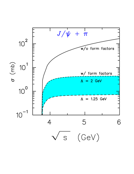
FIG. 7.: The value of the total inclusive $J/\psi$ + $\pi$ inelastic cross section, and its sensitivity to our choices of the form factor parameter $\Lambda$.

The elastic cross section of the $J/\psi$ with the $\omega$ which was shown in Fig. 6 is also drastically affected by form factor considerations. This is displayed in Fig. 8. Note that the suppression due to the form factor is different in the elastic and inelastic cases, owing to different kinematics.

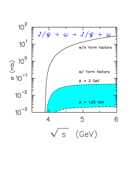
FIG. 8.: The value of the $J/\psi$ + $\omega$ elastic cross section, and its sensitivity to our choices of the form factor parameter $\Lambda$. The solid curve is obtained without form factors, the dashed curves mark the limits of our range in form factors.

FIG. 9.: The value of the total inclusive $J/\psi$ + $\rho$ inelastic cross section, and its sensitivity to our choices of the form factor parameter $\Lambda$.

Finally we also show the total inclusive cross section for rho-induced absorption of the $J/\psi$ in Fig. 9. It is worth noting that the upper choice of our form factor parameter has a large energy limit of $\approx$ 1 mb. Using the methods just outlined, we have estimated also $J/\psi+\eta\to\eta_{c}+\phi$ (0.06 mb), $J/\psi+K\to\eta_{c}+K_{1}$ (0.18 mb). The numbers in parentheses refer to cross section values that are approximately in the centre of the form factor window. To our knowledge, those channels also have not been discussed previously.

V The $J$/$\psi$ spectral function

For hadrons immersed in a strongly interacting medium, one finds that two-loop effects dominate over one-loop effects in the calculations of imaginary parts of particle propagators [31]. This owes largely to the size of the coupling in the confined sector. We have verified that this is the case here also, by doing explicit calculations. Thus, we neglect one-loop effects. We will also neglect effects on the real part of the $J/\psi$ propagator. We thus will assume that the $J/\psi$ will suffer negligible mass-shifts. We partly base this reasoning on the large mass of the charmonium vector meson. Also, recent calculations of $J/\psi$ properties in nuclear matter do yield mass shifts that are small [32].

Our first task is then to calculate the broadening due to collisions of the $J/\psi$ with particles that make up the heat bath. The width induced by a reaction of the type $J/\psi\,2\rightarrow 34$, where 2, 3, and 4 are arbitrary species is [31, 33].

$$\Gamma(\omega,\vec{p})\ =\ \frac{1}{2\omega}\int\,d\Omega\,n_{2}(E_{2})(1+n_{3}(E_{3}))(1+n_{4}(E_{4}))|\overline{{\cal M}(J/\psi 2\rightarrow 34)}|^{2}\ ,$$ (30)

where $\omega\ =\ \sqrt{\vec{p\,}^{2}+m_{J/\psi}^{2}}$, $\vec{p}$ being the three-vector of the $J/\psi$. Note that 3 or 4 can be a $J/\psi$. In Eq. (30),

$$d\Omega\ =\ d\bar{p}_{2}d\bar{p}_{3}d\bar{p}_{4}(2\pi)^{4}\delta(p+p_{2}-p_{3}-p_{4}),$$ (31)

and

$$d\bar{p}_{i}\ =\ \frac{d^{3}p_{i}}{(2\pi)^{3}\,2E_{i}}\ .$$ (32)

The reactions we consider will involve only mesons. In principle, a $J/\psi$ can also be produced by an inverse reaction involving particles from the thermal background [33]. Here, phase space considerations make the inverse channel negligible.

We write the spectral function of the $J/\psi$ as

$$A_{J/\psi}(\omega,\vec{p\,})\ =\ -2{\rm Im}D_{J/\psi}(\omega,\vec{p\,})\ ,$$ (33)

where $D_{J/\psi}$ is the scalar part of the $J/\psi$ propagator. Neglecting the difference between longitudinal and transverse polarizations of the $J/\psi$ in the finite temperature medium [34], one has

$$D_{J/\psi}(\omega,\vec{p\,})\ =\ \frac{1}{p^{2}-m_{J/\psi}^{2}-F(\omega,\vec{p\,})}\ ,$$ (34)

where $p^{\mu}=(\omega,\vec{p\,})$, and $F$ is the scalar imaginary self-energy. Then, using

$$\Gamma_{J/\psi}=-1/m_{J/\psi}~{}{\rm Im}~{}F({p^{2}}=m_{J/\psi}^{2})$$ (35)

one can write in the on-shell approximation

$$A_{J/\psi}(\omega,\vec{p\,})\ =\ \frac{2\,m_{J/\psi}\,\Gamma_{J/\psi}}{(p^{2}-m_{J/\psi}^{2})^{2}+m_{J/\psi}^{2}\Gamma_{J/\psi}^{2}}\ ,$$ (36)

where $\Gamma_{J/\psi}$ contains all the contributions we have discussed so far: the vacuum width and the contributions from elastic and inelastic collisions.

One can first shown the effects of purely elastic processes on the $J/\psi$ spectral function. This appears in Fig. 10. Note that $\Lambda$ = 2 Gev throughout this section, keeping in mind any investigation of a more quantitative nature will need to reflect the possible ambiguities in this choice that were discussed earlier.

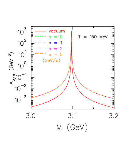
FIG. 10.: Spectral function in vacuum and at finite temperature allowing only elastic scattering.

Without inclusion of the elastic scattering with $\omega$’s through $\eta_{c}$ exchange, the spectral function deviates so little from the vacuum that all curves lie on top of one another. But as one can see in Fig.10, elastic scattering in the medium now has a non negligible effect and distorts the spectral function. Since the $J/\psi+\omega$ cross section with form factors is quite flat in $\sqrt{s}$, the momentum dependence here is not important.

Let us now consider the $J/\psi$ charmonium state traveling in a finite temperature gas first consisting only of $\pi$’s, $K$’s and $\rho$’s. The spectral function at two temperatures, 150 and 200 MeV, is shown in Figs. 11 and 12. One notices a substantial broadening of the spectral distribution, along with a suppression of the peak. This considerable effect is even more pronounced at the higher temperature. If we include all the inelastic processes we have considered in this work (summarized in Table II), it turns out the quantitative differences between results involving all those and the ones shown in Fig. 11 and 12 are small and can be neglected. Clearly, the $\pi$’s, $K$’s, and $\rho$’s play the leading role.

FIG. 11.: Spectral function in vacuum and at $T$ = 150 MeV temperature allowing inelastic interactions with $\pi$’s, $K$’s and $\rho$’s.

FIG. 12.: Spectral function in vacuum and at 200 MeV temperature allowing inelastic interactions with $\pi$’s, $K$’s and $\rho$’s.

VI Conclusion

In this work, cross sections for the interactions of the $J/\psi$ with light mesons were evaluated. It has been found that those cross sections are all quite different, and also not constant with respect to the energy of the colliding particles. The form factors that are germane to meson exchange models such as the one discussed here have been constrained by hadronic phenomenology, Lorentz invariance and electromagnetic gauge invariance. The numerical effect of those form factors are large and therefore a careful treatment is mandatory. The importance of the $J/\psi+\pi\to X$ hadronic absorption channel has been highlighted, especially those that invole the $\eta_{c}$. Similarly, the elastic cross section involving an external $\omega$ interacting through an exchanged $\eta_{c}$ is found to be appreciable. Those findings should have some effect on the hadronic phenomenology that is an ingredient to the theoretical modeling of high energy heavy ion collisions. Specifically, the $J/\psi+\pi$ inelastic channel can be interpreted as the leading contribution in the $J/\psi$ absorption by “comovers”. In this light, the average value of our comover cross section just about reaches 2 mb. If one consider the $J/\psi+\rho$ channel, one could even add an additional mb. A recent study uses $\sigma_{\rm comovers}$ = 1 mb [9]. It is important for values obtained phenomenologically and for those based on more microscopic approaches to eventually meet. The studies performed here however do point to the richness of the many-body problem. Several reactions channels have been considered and even more work needs to be done in order to complete the survey of what turns out to be a vast hadronic landscape. Our exploration continues.

We have evaluated the spectral function for a $J/\psi$ state traveling in a finite temperature gas of mesons. We have found that the spectral function gets considerably modified, owing mainly to inelastic interactions with the constituents of the hot meson gas.

For the moment, we have refrained from attempting a detailed comparison with heavy ion data. It is also clear that such an application will require great care. For example it is claimed here that the absorption of the $J/\psi$ on pions is important, especially when the $\eta_{c}$ is part of the final state. However, inverse reactions can produce a $J/\psi$: $\eta_{c}+\rho\to J/\psi+\pi$ (0.7 mb), and $\eta_{c}+\pi\to J/\psi+\rho$ (2 mb). The numbers in parentheses refer to cross section values that are approximately in the centre of the form factor window. One therefore needs to advocate a careful simulation of the nuclear collision, with the inclusion of the relevant important reaction channels and of their detailed balance partners. This work is extensive, has begun, and will be reported on elsewhere. It is first necessary to place the interactions of the $J/\psi$ in a proper many-body setting, at the appropriate level of sophistication our current understanding of hadronic physics requires. This also implies pointing out the caveats as well as the successes.

Appendix: Gauge Invariance

The amplitudes discussed in this work that couple to vector mesons that have the quantum number of the photon need to obey gauge invariance in the electromagnetic sector, or more specifically current conservation. This statement is an immediate consequence of Vector Meson Dominance. We focus for the moment on the reaction $J/\psi(p_{1})+\pi(p_{2})\to D^{*}(p_{3})+\bar{D}(p_{4})$. The invariant amplitude emerging from Eq. 26 is ${\cal M\/}={\cal M\/}_{1}+{\cal M\/}_{2}+{\cal M\/}_{3}$ where

$${\cal M\/}_{1} = {\sqrt{2\over 3}}g^{2}\,\epsilon^{\mu}(p_{1})(2p_{4}-p_{1})_{\mu}{1\over(p_{1}-p_{4})^{2}-m_{4}^{2}}(2p_{2}-p_{3})_{\nu}\epsilon^{\nu}(p_{3})$$ (A1)

$${\cal M\/}_{2} = {\sqrt{2\over 3}}g^{2}\,\epsilon^{\mu}(p_{1})\left[(2p_{3}-p_{1})_{\mu}\,g_{\nu\alpha}\,-\,(p_{1}+p_{3})_{\alpha}\,g_{\mu\nu}\,+\,(2p_{1}-p_{3})_{\nu}\,g_{\mu\alpha}\right]$$ (A2)

$$\times{\left[-g^{\alpha\beta}+(p_{1}-p_{3})^{\alpha}(p_{1}-p_{3})^{\beta}/m_{3}^{2}\right]\over(p_{1}-p_{3})^{2}-m_{3}^{2})}(p_{2}+p_{4})_{\beta}\epsilon^{\nu}(p_{3})$$ (A3)

$${\cal M\/}_{3} = {\sqrt{2\over 3}}g^{2}\,\epsilon^{\mu}(p_{1})\left[-g_{\mu\nu}\right]\epsilon^{\nu}(p_{3}).$$ (A4)

Gauge invariance requires that ${\cal{M}\,}\left(\epsilon^{\mu}(p_{1})\to p_{1}^{\mu}\right)$ must be identically zero. In particular, it must vanish for arbitrary choices of pseudoscalar and vector masses.

Replacing $\epsilon^{\mu}(p_{1})\to p_{1}^{\mu}$, and doing the contraction gives

$${\cal M\/}_{1} = {\sqrt{2\over 3}}g^{2}\,\left[-(2p_{2}-p_{3})_{\nu}\right]\,\epsilon^{\nu}(p_{3})$$ (A5)

$${\cal M\/}_{2} = {\sqrt{2\over 3}}g^{2}\,\left\{(p_{2}+p_{4})_{\nu}+{1\over(p_{1}-p_{3})^{2}-m_{3}^{2}}\left[{(2p_{3}-p_{1})\cdot p_{1}(p_{1}-p_{3})\cdot(p_{2}+p_{4})(p_{1}-p_{3})_{\nu}\over m_{3}^{2}}\right.\right.$$ (A6)

$$+(p_{1}+p_{3})\cdot(p_{2}+p_{4})(p_{1})_{\nu}-{(p_{1}+p_{3})\cdot(p_{1}-p_{3})(p_{1}-p_{3})\cdot(p_{2}+p_{4})(p_{1})_{\nu}\over m_{3}^{2}}$$ (A7)

$$\left.\left.-(2p_{1}-p_{3})_{\nu}(p_{1})\cdot(p_{2}+p_{4})+{(2p_{1}-p_{3})_{\nu}(p_{1})\cdot(p_{1}-p_{3})(p_{1}-p_{3})\cdot(p_{2}+p_{4})\over m_{3}^{2}}\right]\right\}\,\epsilon^{\nu}(p_{3})$$ (A8)

$${\cal M\/}_{3} = {\sqrt{2\over 3}}g^{2}\,\left[-(p_{1})_{\nu}\right]\epsilon^{\nu}(p_{3}).$$ (A9)

We note that ${\cal M\/}_{1}$ plus the first term in ${\cal M\/}_{2}$, plus ${\cal M\/}_{3}$ vanishes due to energy-momentum conservation. The remaining pieces from ${\cal M\/}_{2}$ are

$$\propto {1\over m_{3}^{2}\left[(p_{1}-p_{3})^{2}-m_{3}^{2}\right]}{\{}(2p_{3}-p_{1})\cdotp_{1}(p_{1}-p_{3})\cdot(p_{2}+p_{4})(p_{1}-p_{3})_{\nu}+m_{3}^{2}(p_{1}+p_{3})\cdot(p_{2}+p_{4})(p_{1})_{\nu}$$ (A10)

$$-(p_{1}+p_{3})\cdot(p_{1}-p_{3})(p_{1}-p_{3})\cdot(p_{2}+p_{4})(p_{1})_{\nu}-m_{3}^{2}(2p_{1}-p_{3})_{\nu}p_{1}\cdot(p_{2}+p_{4})$$ (A11)

$$+(2p_{1}-p_{3})_{\nu}p_{1}\cdot(p_{1}-p_{3})(p_{1}-p_{3})\cdot(p_{2}+p_{4}){\}}\,\epsilon^{\nu}(p_{3})$$ (A12)

Terms proportional to $(p_{3})_{\nu}$ vanish when contracted with $\epsilon^{\nu}(p_{3})$ due to transversality. Thus, the surviving terms can be written as

$$\propto {(p_{1})_{\nu}\over m_{3}^{2}\left[(p_{1}-p_{3})^{2}-m_{3}^{2}\right]}{\{}(2p_{3}-p_{1})\cdot(p_{1})(p_{4}-p_{2})\cdot(p_{2}+p_{4})+m_{3}^{2}(p_{1}+p_{3})\cdot(p_{2}+p_{4})$$ (A13)

$$+m_{3}^{2}(-2p_{1})\cdot(p_{2}+p_{4})-(p_{1}+p_{3})\cdot(p_{1}-p_{3})(p_{4}-p_{2})\cdot(p_{2}+p_{4})+2(p_{1})\cdot(p_{1}-p_{3})(p_{4}-p_{2})\cdot(p_{2}+p_{4}){\}}\,\epsilon^{\nu}$$ (A14)

Finally, we can simplify to

$$\propto (p_{1})_{\nu}{\{}(m_{4}^{2}-m_{2}^{2})\left[m_{3}^{2}\right]+m_{3}^{2}\left[(p_{3}-p_{1})\cdot(p_{2}+p_{4})\right]{\}}\,\epsilon^{\nu}(p_{3})$$ (A15)

$$= (p_{1})_{\nu}{\{}m_{3}^{2}(m_{4}^{2}-m_{2}^{2})+m_{3}^{2}(p_{2}-p_{4})\cdot(p_{2}+p_{4}){\}}\,\epsilon^{\nu}(p_{3})$$ (A16)

$$= (p_{1})_{\nu}{\{}m_{3}^{2}{\{}m_{4}^{2}-m_{2}^{2}+m_{2}^{2}-m_{4}^{2}{\}}$$ (A17)

$$= 0.$$ (A18)

Indeed, current is conserved in the general case. The other channels can similarly be shown to conserve current.

TABLE I.: Model prediction for widths. The phenomenological approach refers to that of Refs. [11, 13, 14].

particle	chiral model	pheno. model	experiment
K∗(892)0	44.5 MeV	97.0 MeV	50.5 $\pm$ 0.6 MeV
K∗(892)±	44.5 MeV	97.0 MeV	49.8 $\pm$ 0.8 MeV
D∗(2007)0	10.1 keV	22.0 KeV	$<$ 2.1 MeV, 90% CL
D∗(2010)±	21.1 keV	46.0 KeV	$<$ 131 keV, 90% CL

TABLE II.: We list here the hadronic reactions involving $J/\psi$ that were considered in this work. It is implied that the figures also include the Hermitian conjugate inelastic final state when it is different from the one listed below.

Elastic channels		Inelastic channels
		initial state	final state
$J/\psi+\pi$		$J/\psi+\pi$	$D^{*}+\bar{D}$
$J/\psi+\eta$		$J/\psi+\pi$	$\eta_{c}+\rho$
$J/\psi+K$		$J/\psi+\pi$	$\eta_{c}+b_{1}$
$J/\psi+\rho$		$J/\psi+\eta$	$D^{*}+\bar{D}$
$J/\psi+\omega$		$J/\psi+\eta$	$\eta_{c}+\phi$
$J/\psi+\phi$		$J/\psi+K$	$D_{s}+\bar{D^{*}}$
		$J/\psi+\rho$	$D+\bar{D}$
		$J/\psi+\rho$	$D^{*}+\bar{D^{*}}$
		$J/\psi+\rho$	$\eta_{c}+\pi$
		$J/\psi+\omega$	$D+\bar{D}$
		$J/\psi+\omega$	$D^{*}+\bar{D^{*}}$
		$J/\psi+\phi$	$D+\bar{D}$
		$J/\psi+\phi$	$D^{*}+\bar{D^{*}}$
		$J/\psi+K$	$\eta_{c}+K_{1}$
		$J/\psi+K^{*}$	$D_{s}+\bar{D}$
		$J/\psi+K^{*}$	$D_{s}^{*}+\bar{D^{*}}$

REFERENCES

- [1] See, for example, Proceedings of Quark Matter ’99, edited by L. Riccati, M. Masera, and E. Vercellin, Nucl Phys. A661, 1c (1999), and references therein.
- [2] T. Matsui and H. Satz, Phys. Lett. B178, 416 (1986).
- [3] Xiao-Ming Xu, D. Kharzeev, H. Satz, and Xin-Nian Wang, Phys. Rev. C 53, 3051 (1996).
- [4] C. Baglin et al., Phys. Lett. B220, 471 (1989); B345, 617 (1995); M. C. Abreu et al., Nucl. Phys. A544, 209c (1992).
- [5] S. Gavin and R. Vogt, Nucl. Phys. B345, 104 (1990); C. Gerschel and J. Hüfner, Nucl. Phys. A544, 513c (1992); R. Vogt, Phys. Rep. 310, 197 (1999).
- [6] C. Gale, S. Jeon, and J. Kapusta, hep-ph/9912213.
- [7] See, for example, D. Kharzeev, Nucl. Phys. A638, 279c (1998), and references therein.
- [8] N. Armesto, A. Capella, and E. G. Ferreiro, Phys. Rev. C 59, 395 (1999); C. Spieles et al., Phys. Lett. B458, 137 (1999).
- [9] A. Capella, E. G. Ferreiro, and A. B. Kaidalov, Phys. Rev. Lett. 85, 2080 (2000).
- [10] D. Kharzeev and H. Satz, Phys. Lett. B334, 155 (1994); K. Martin, D. Blaschke, and E. Quack, Phys. Rev. C 51, 2723 (1995); S. G. Matinyan and B. Müller, Phys. Rev. C 58, 2994 (1998).
- [11] S. G. Matinyan and B. Müller, Phys. Rev. C 58, 2994 (1998).
- [12] P. Braun-Munzinger and K. Redlich, Proceedings of the 14th International Conference on Ultrarelativistic Nucleus-Nucleus Collisions (QM 99), Torino, Italy, 10-15 May 1999, Nucl. Phys. A661, 546c (1999).
- [13] Kevin L. Haglin, Phys. Rev. C 61, 031902 (2000).
- [14] Z. Lin and C.M. Ko, Phys. Rev. C 62, 034903 (2000).
- [15] See, for example, W. Greiner and B. Müller, Quantum Mechanics: Symmetries (Springer, Berlin, 1989).
- [16] Ö. Kaymakcalan and J. Schecter, Rev. D 31, 1109 (1985).
- [17] P. Colangelo, F. De Fazio and G. Nardulli, Phys. Lett. B278, 480 (1994).
- [18] M. A. Ivanov, Y. L Kalinovsky and C. Roberts, Phys. Rev. D 60, 034018 (1999).
- [19] F.S. Navarra, M. Nielsen, M.E. Bracco, M. Chiapparni and C. L. Schat, hep-ph/0005026.
- [20] P. Colangelo, F. De Fazio, G. Nardulli, Phys. Lett. B 334, 175 (1994).
- [21] We examine here some claim made in the recent literature [14]. The Lagrangian used here (Eq. (26)) is formally equivalent to that in Eq. (6) of Ref. [14], the reader can be convinced by inspection. With the “phenomenological” version of our approach (as explained in the text), our total and cross sections (our Fig. 5) are identical to those in Fig. 2 of Ref. [14]. As correctly pointed out in the latter reference, Ref. [13] does contain typos that make an identification with the approach used here and in Ref. [14] difficult. However, those typos have not propagated to the calculations. What was calculated in Ref. [13] for the cross section was a partial cross section, for a given charged state of the participating fields. There are four such channels. The result of Ref. [13] multiplied by four is equivalent to the one obtained here and to that of [14].
- [22] E. Shuryak and D. Teaney, Phys. Lett. B430, 37 (1998).
- [23] Kim Maltman and Nathan Isgur, Phys. Rev. D 29, 952 (1984).
- [24] R. Kokoski and N. Isgur, Phys. Rev. D 35, 907 (1987).
- [25] See, for example, H. G. Blundell and S. Godfrey, Phys. Rev. D 53, 3700 (1996), and references therein.
- [26] D.E. Groom et al., Eur. Phys. J. C 15, 1 (2000).
- [27] R. Machleidt, K. Holinde, and C. Elster, Phys. Rep. 149, 1 (1987).
- [28] T. H. Bauer et al., Rev. Mod. Phys. 50, 261 (1978).
- [29] K. Redlich, H. Satz, and G. M. Zinovjev, hep-ph/0003079.
- [30] C. Y. Wong, E. S. Swanson, and T. Barnes, Phys. Rev. C 62, 045201 (2000).
- [31] Kevin Haglin, Nucl. Phys. A584, 719 (1995).
- [32] Frank Klingl, Sungsik Kim, Su Houng Lee, Philippe Morath, Wolfram Weise, Phys. Rev. Lett. 82, 3396 (1999); Arata Hayashigaki, Prog. Theor. Phys. 101, 923 (1999).
- [33] H. A. Weldon, Z. Phys. C54, 431 (1992); S. Gao, C. Gale, C. Ernst, H. Stöcker, and W. Greiner, nucl-th/9812059.
- [34] Charles Gale and Joseph Kapusta, Nucl. Phys. B357, 65 (1991).