Introduction to Effective Field Theory

1 Introduction

The basic idea behind effective field theory (EFT) methods is to describe nature in terms of a fully consistent quantum field theory, but one which is valid in a limited energy range. Now strictly speaking this means that almost any theory is an EFT except string theories that try to be a theory of everything (TOE). Indeed even the quintessential quantum field theory—quantum electrodynamics—is an EFT in that it must break down at the very highest energies. In fact we represent the high energy contribution in terms of a conterterm which, together with the divergent component from the loop integration, we fit in terms of the experimental mass and charge.

In order to get a better feel for this idea it is useful to consider a simpler example from the regime of ordinary quantum mechanics—that of Rayleigh scattering, or why the sky is blue.

1.1 Rayleigh Scattering

Before proceeding to QCD, let’s first examine effective field theory in the simpler context of ordinary quantum mechanics, in order to get familiar with the idea. Specifically, we examine the question of why the sky is blue, whose answer can be found in an analysis of the scattering of photons from the sun by atoms in the atmosphere—Compton scattering.[1] First we examine the problem using traditional quantum mechanics and, for simplicity, consider elastic (Rayleigh) scattering from single-electron (hydrogen) atoms. The appropriate Hamiltonian is then

$$H={(\vec{p}-e\vec{A})^{2}\over 2m}+e\phi$$ (1)

and the leading—${\cal O}(e^{2})$—amplitude for Compton scattering is given by the Feynman diagrams shown in Figure 1 as

$${\rm Amp} = -{e^{2}/m\over\sqrt{2\omega_{i}2\omega_{f}}}\left[\hat{\epsilon}_{i}\cdot\hat{\epsilon}_{f}^{*}+{1\over m}\sum_{n}\left({\hat{\epsilon}_{f}^{*}\cdot<0|\vec{p}e^{-i\vec{q}_{f}\cdot\vec{r}}|n>\hat{\epsilon}_{i}\cdot<n|\vec{p}e^{i\vec{q}_{i}\cdot\vec{r}}|0>\over\omega_{i}+E_{0}-E_{n}}\right.\right.$$ (2)

$$+ \left.\left.{\hat{\epsilon}_{i}\cdot<0|\vec{p}e^{i\vec{q}_{i}\cdot\vec{r}}|n>\hat{\epsilon}_{f}^{*}\cdot<n|\vec{p}e^{-i\vec{q}_{f}\cdot\vec{r}}|0>\over E_{0}-\omega_{f}-E_{n}}\right)\right]$$

where $|0>$ represents the hydrogen ground state having binding energy $E_{0}$.

Figure 1: Feynman diagrams contributing to low energy Compton scattering.

(Note that for simplicity we take the proton to be infinitely heavy so it need not be considered.) Here the leading component is the familiar $\omega$-independent Thomson amplitude and would appear naively to lead to an energy-independent cross-section. However, this is not the case. Indeed, as shown in a homework problem, provided that the energy of the photon is much smaller than a typical excitation energy—as is the case for optical photons—the cross section can be written as

$$\quad{d\sigma\over d\Omega} = \lambda^{2}\omega^{4}|\hat{\epsilon}_{f}^{*}\cdot\hat{\epsilon}_{i}|^{2}\left(1+{\cal O}\left({\omega^{2}\over(\Delta E)^{2}}\right)\right)$$ (3)

where

$$\lambda=\alpha_{em}\sum{2|z_{n0}|^{2}\over E_{n}-E_{0}}$$ (4)

is the atomic electric polarizability, $\alpha_{em}=e^{2}/4\pi$ is the fine structure constant, and $\Delta E\sim m\alpha_{em}^{2}$ is a typical hydrogen excitation energy. We note that $\alpha_{em}\lambda\sim a_{0}^{2}\times{\alpha_{em}\over\Delta E}\sim a_{0}^{3}$ is of order the atomic volume, as will be exploited below and that the cross section itself has the characteristic $\omega^{4}$ dependence which leads to the blueness of the sky—blue light scatters much more strongly than red.[2]

Now while the above derivation is certainly correct, it requires somewhat detailed and lengthy quantum mechanical manipulations which obscure the relatively simple physics involved. One can avoid these problems by the use of effective field theory methods outlined above. The key point is that of scale. Since the incident photons have wavelengths $\lambda\sim 5000$A much larger than the $\sim$ 1A atomic size, then at leading order the photon is insensitive to the presence of the atom, since the latter is electrically neutral. If $\chi$ represents the wavefunction of the atom then the effective leading order Hamiltonian is simply that for the hydrogen atom

$$H_{eff}^{(0)}=\chi^{*}\left({\vec{p}^{2}\over 2m}+e\phi\right)\chi$$ (5)

and there is no interaction with the field. In higher orders, there can exist such atom-field interactions and this is where the effective Hamiltonian comes in to play. In order to construct the effective interaction, we demand certain general principles—the Hamiltonian must satisfy fundamental symmetry requirements. In particular $H_{eff}$ must be gauge invariant, must be a scalar under rotations, and must be even under both parity and time reversal transformations. Also, since we are dealing with Compton scattering, $H_{eff}$ must be quadratic in the vector potential. Actually, from the requirement of gauge invariance it is clear that the effective interaction should involve only the electric and magnetic fields

$$\vec{E}=-\vec{\nabla}\phi-{\partial\over\partial t}\vec{A},\qquad\vec{B}=\vec{\nabla}\times\vec{A}$$ (6)

since these are invariant under a gauge transformation

$$\phi\rightarrow\phi+{\partial\over\partial t}\Lambda,\qquad\vec{A}\rightarrow\vec{A}-\vec{\nabla}\Lambda$$ (7)

while the vector and/or scalar potentials are not. The lowest order interaction then can involve only the rotational invariants $\vec{E}^{2},\vec{B}^{2}$ and $\vec{E}\cdot\vec{B}$. However, under spatial inversion—$\vec{r}\rightarrow-\vec{r}$—electric and magnetic fields behave oppositely—$\vec{E}\rightarrow-\vec{E}$ while $\vec{B}\rightarrow\vec{B}$—so that parity invariance rules out any dependence on $\vec{E}\cdot\vec{B}$. Likewise under time reversal—$t\rightarrow-t$ we have $\vec{E}\rightarrow\vec{E}$ but $\vec{B}\rightarrow-\vec{B}$ so such a term is also ruled out by time reversal invariance. The simplest such effective Hamiltonian must then have the form

$$H_{eff}^{(1)}=\chi^{*}\chi[-{1\over 2}c_{E}\vec{E}^{2}-{1\over 2}c_{B}\vec{B}^{2}]$$ (8)

(Forms involving time or spatial derivatives are much smaller.) We know from electrodynamics that ${1\over 2}(\vec{E}^{2}+\vec{B}^{2})$ represents the field energy per unit volume, so by dimensional arguments, in order to represent an energy in Eq. 8, $c_{E},c_{B}$ must have dimensions of volume. Also, since the photon has such a long wavelength, there is no penetration of the atom, so only classical scattering is allowed. The relevant scale must then be atomic size so that we can write

$$c_{E}=k_{E}a_{0}^{3},\qquad c_{B}=k_{B}a_{0}^{3}$$ (9)

where we expect $k_{E},k_{B}\sim{\cal O}(1)$. Finally, since for photons with polarization $\hat{\epsilon}$ and four-momentum $q_{\mu}$ we identify $\vec{A}(x)=\hat{\epsilon}\exp(-iq\cdot x)$ then from Eq. 6, $|\vec{E}|\sim\omega$, $|\vec{B}|\sim|\vec{k}|=\omega$ and

$${d\sigma\over d\Omega}\propto|<f|H_{eff}|i>|^{2}\sim\omega^{4}a_{0}^{6}$$ (10)

as found in the previous section via detailed calculation.

We see from this example the strength of the effective interaction procedure—allowing access to the basic physics with very little formal work.

2 Chiral Perturbation Theory

An important example within the realm of quantum field theory is that of chiral perturbation theory. In this case we apply these ideas to the case of QCD. Since back in prehistoric times the holy grail of particle/nuclear physicists has been to construct a theory of elementary particle interactions which emulates quantum electrodynamics in that it is elegant, renormalizable, and phenomenologically successful. We now have a theory which satisfies two out of the three criteria—quantum chromodynamics (QCD). Indeed the form of the Lagrangian

$${\cal L}_{\mbox{\tiny QCD}}=\bar{q}(i{\not\!\!D}-m)q-{1\over 2}{\rm tr}\;G_{\mu\nu}G^{\mu\nu}\,.$$ (13)

is elegantly simple, and the theory is renormalizable. So why are we still not satisfied? The difficulty lies with the third criterion—phenomenological success. While at the very largest energies, asymptotic freedom allows the use of perturbative techniques, for those who are interested in making contact with low energy experimental findings there exist at least three fundamental difficulties:

• QCD is written in terms of the ”wrong” degrees of freedom—quarks and gluons—while experiments are performed with hadronic bound states;

• the theory is hopelessly non-linear due to gluon self interaction;

• the theory is one of strong coupling—$g^{2}/4\pi\sim 1$—so that perturbative methods are not practical.

Nevertheless, there has been a great deal of recent progress in making contact between theory and experiment at low energies using effective field theory and chiral symmetry.[3]

The idea of ”chirality” is defined by the projection operators $\Gamma_{L,R}={1\over 2}(1\pm\gamma_{5})$ which project left- and right-handed components of the Dirac wavefunction. In terms of chirality states the quark component of the QCD Lagrangian can be written as

$$\bar{q}(i\not\!\!D-m)q=\bar{q}_{L}i\not\!\!Dq_{L}+\bar{q}_{R}i\not\!\!Dq_{R}-\bar{q}_{L}mq_{R}-\bar{q}_{R}mq_{L}$$ (14)

and in the limit in which the light (u,d,s) quark masses are set to zero QCD is seen to have an exact $SU(3)_{L}\times SU(3)_{R}$ invariance. Of course, it is known that the axial part of this symmetry is broken spontaneously in which case Goldstone’s theorem requires the existence of eight massless pseudoscalar bosons, which couple derivatively to the rest of the universe. Of course, in the real world such massless $0^{-}$ states do not exist, since exact chiral invariance is broken by the small quark mass terms. Thus what we have in reality are eight very light (but not massless) pseudo-Goldstone bosons which make up the pseudoscalar octet. Since such states are lighter than their other hadronic counterparts, we have a situation wherein effective field theory can be applied—provided one is working at energy-momenta small compared to the $\sim 1$ GeV scale which is typical of hadrons, one can describe the interactions of the pseudoscalar mesons using an effective Lagrangian. Actually this has been known since the 1960’s, where a good deal of work was done with a lowest order effective chiral Lagrangian[4]

$${\cal L}_{2}={F_{\pi}^{2}\over 4}\mbox{Tr}(\partial_{\mu}U\partial^{\mu}U^{\dagger})+{m^{2}_{\pi}\over 4}F_{\pi}^{2}\mbox{Tr}(U+U^{\dagger})\,.$$ (15)

where the subscript 2 indicates that we are working at two-derivative order or one power of chiral symmetry breaking—i.e. $m_{\pi}^{2}$. Here $U\equiv\exp(\sum\lambda_{i}\phi_{i}/F_{\pi})$, where $F_{\pi}=92.4$ is the pion decay constant. This Lagrangian is unique. It also has predictive power. Expanding to second order in the fields we find the well known Gell-Mann-Okubo formula for pseudoscalar masses[5]

$$3m_{\eta}^{2}+m_{\pi}^{2}-4m_{K}^{2}=0\,\,.$$ (16)

and is well-satisfied experimentally. Expanding to fourth order in the fields we also reproduce the well-known and experimentally successful Weinberg $\pi\pi$ scattering lengths.

However, when one attempts to go beyond tree level, in order to unitarize the results, divergences arise and that is where the field stopped at the end of the 1960’s. The solution, as proposed a decade later by Weinberg[6] and carried out by Gasser and Leutwyler[7], is to absorb these divergences in phenomenological constants, just as done in QED. What is different in this case is that the theory is nonrenormalizabile in that the forms of the divergences are different from the terms that one started with. That means that the form of the counterterms that are used to absorb these divergences must also be different, and Gasser and Leutwyler wrote down the most general counterterm Lagrangian that one can have at one loop, involving four-derivative interactions

$${\cal L}_{4} = \sum^{10}_{i=1}L_{i}{\cal O}_{i}=L_{1}\bigg{[}{\rm tr}(D_{\mu}UD^{\mu}U^{\dagger})\bigg{]}^{2}+L_{2}{\rm tr}(D_{\mu}UD_{\nu}U^{\dagger})\cdot{\rm tr}(D^{\mu}UD^{\nu}U^{\dagger})$$

$$+ L_{3}{\rm tr}(D_{\mu}UD^{\mu}U^{\dagger}D_{\nu}UD^{\nu}U^{\dagger})+L_{4}{\rm tr}(D_{\mu}UD^{\mu}U^{\dagger}){\rm tr}(\chi{U^{\dagger}}+U{\chi}^{\dagger})$$

$$+ L_{5}{\rm tr}\left(D_{\mu}UD^{\mu}U^{\dagger}\left(\chi U^{\dagger}+U\chi^{\dagger}\right)\right)+L_{6}\bigg{[}{\rm tr}\left(\chi U^{\dagger}+U\chi^{\dagger}\right)\bigg{]}^{2}$$

$$+ L_{7}\bigg{[}{\rm tr}\left(\chi^{\dagger}U-U\chi^{\dagger}\right)\bigg{]}^{2}+L_{8}{\rm tr}\left(\chi U^{\dagger}\chi U^{\dagger}+U\chi^{\dagger}U\chi^{\dagger}\right)$$

$$+ iL_{9}{\rm tr}\left(F^{L}_{\mu\nu}D^{\mu}UD^{\nu}U^{\dagger}+F^{R}_{\mu\nu}D^{\mu}U^{\dagger}D^{\nu}U\right)+L_{10}{\rm tr}\left(F^{L}_{\mu\nu}UF^{R\mu\nu}U^{\dagger}\right)$$

where the covariant derivative is defined via

$$D_{\mu}U=\partial_{\mu}U+\{A_{\mu},U\}+[V_{\mu},U]$$ (18)

the constants $L_{i},i=1,2,\ldots 10$ are arbitrary (not determined from chiral symmetry alone) and $F^{L}_{\mu\nu},F^{R}_{\mu\nu}$ are external field strength tensors defined via

$$F^{L,R}_{\mu\nu}=\partial_{\mu}F^{L,R}_{\nu}-\partial_{\nu}F^{L,R}_{\mu}-i[F^{L,R}_{\mu},F^{L,R}_{\nu}],\qquad F^{L,R}_{\mu}=V_{\mu}\pm A_{\mu}.$$ (19)

Now just as in the case of QED the bare parameters $L_{i}$ which appear in this Lagrangian are not physical quantities. Instead the experimentally relevant (renormalized) values of these parameters are obtained by appending to these bare values the divergent one-loop contributions—

$$L^{r}_{i}=L_{i}-{\gamma_{i}\over 32\pi^{2}}\left[{-2\over\epsilon}-\ln(4\pi)+\gamma-1\right]$$ (20)

By comparing predictions with experiment, Gasser and Leutwyler were able to determine empirical numbers for each of these ten parameters. Typical values are shown in Table 1, together with the way in which they were determined.

Coefficient	Value	Origin
$L_{1}^{r}$	$0.65\pm 0.28$	$\pi\pi$ scattering
$L_{2}^{r}$	$1.89\pm 0.26$	and
$L_{3}^{r}$	$-3.06\pm 0.92$	$K_{\ell 4}$ decay
$L_{5}^{r}$	$2.3\pm 0.2$	$F_{K}/F_{\pi}$
$L_{9}^{r}$	$7.1\pm 0.3$	$\pi$ charge radius
$L_{10}^{r}$	$-5.6\pm 0.3$	$\pi\rightarrow e\nu\gamma$

Table 1: Gasser-Leutwyler counterterms and the means by which they are determined.

The important question to ask at this point is why stop at order four derivatives? Clearly if two-loop amplitudes from ${\cal L}_{2}$ or one-loop corrections from ${\cal L}_{4}$ are calculated, divergences will arise which are of six-derivative character. Why not include these? The answer is that the chiral procedure represents an expansion in energy-momentum. Corrections to the lowest order (tree level) predictions from one loop corrections from ${\cal L}_{2}$ or tree level contributions from ${\cal L}_{4}$ are ${\cal O}(E^{2}/\Lambda_{\chi}^{2})$ where $\Lambda_{\chi}\sim 4\pi F_{\pi}\sim 1$ GeV is the chiral scale[8]. Thus chiral perturbation theory is a low energy procedure. It is only to the extent that the energy is small compared to the chiral scale that it makes sense to truncate the expansion at the one-loop (four-derivative) level. Realistically this means that we deal with processes involving $E<500$ MeV, and, for such reactions the procedure is found to work very well.

In fact Gasser and Leutwyler, besides giving the form of the ${\cal O}(p^{4})$ chiral Lagrangian, have also performed the one loop integration and have written the result in a simple algebraic form. Users merely need to look up the result in their paper and, despite having ten phenomenological constants, the theory is quite predictive. An example is shown in Table 2, where predictions are given involving quantities which arise using just two of the constants—$L_{9},L_{10}$. The table also reveals at least one intruguing problem—a solid chiral prediction, that for the charged pion polarizability, is possibly violated although this is not clear since there are three experimental results, only one of which is in disagreement. Clearing up this discrepancy should be a focus of future experimental work. Because of space limitations we shall have to be content to stop here, but interested readers can find applications to other systems in a number of review articles[9].

Reaction	Quantity	Theory	Experiment
$\pi^{+}\rightarrow e^{+}\nu_{e}\gamma$	$h_{V}(m_{\pi}^{-1})$	0.027	$0.029\pm 0.017$[10]
$\pi^{+}\rightarrow e^{+}\nu_{e}e^{+}e^{-}$	$r_{V}/h_{V}$	2.6	$2.3\pm 0.6$[10]
$\gamma\pi^{+}\rightarrow\gamma\pi^{+}$	$(\alpha_{E}+\beta_{M})\,(10^{-4}\,{\rm fm}^{3})$	0	$1.4\pm 3.1$[11]
	$\alpha_{E}\,(10^{-4}\,{\rm fm}^{3})$	2.8	$6.8\pm 1.4$[12]
			$12\pm 20$[13]
			$2.1\pm 1.1$[14]

Table 2: Chiral Predictions and data in radiative pion processes.

3 NN Effective Field Theory

Prompted in part by the success of chiral effective field theories, a number of groups have attempted to extend such programs to the arena of NN scattering. In the standard approach, of course, one assumes the validity of some potential form, chooses parameters in order to match scattering experiments in some energy region and then attemptes to predict phase shifts at other energies. The idea in EFT is similar—at low energies one should be able to express scattering only in terms of observables such as the scattering length and effective range. In terms of potentials, this means that one is characterizing the scattering in terms of the quantities

$$a\simeq-{m_{r}\over 2\pi}U(\vec{p}=0),\quad r_{e}\simeq{1\over 3a^{2}}{m_{r}\over 2\pi}\vec{\nabla}^{2}U(\vec{p}=0)$$ (21)

i.e. in terms of the low energy momentum space potential $U(\vec{p})=\int d^{3}r\exp(i\vec{p}\cdot\vec{r})V(r)$. This suggests the use of simple contact interactions which reproduce these results, and that is the approach used by EFT practitioners. If one is interested only in NN scattering the effective range and EFT results are identical. However, if one wishes to include interactions with external fields, the simple EFT Lagrangian must be supplemented by various undetermined counterterms[17]. For example, in the case of coupling to an electromagnetic field at lowest order one must include two magnetic counterterms, usually called $L_{1},L_{2}$[18]. The coupling $L_{2}$ is found from comparison of the experimental deuteron magnetic moment—0.857 nm—with its simple one-body value—$\mu_{p}+\mu_{n}=0.88$ nm. The coupling $L_{1}$ is determined by comparison of the measured threshold cross section for the radiative capture process $n+d\rightarrow d+\gamma$—$\sigma_{exp}=334.5\pm 0.5$ mb for and incident thermal neutron velocity 2200 m/s—with the lowest order (zero range approximation) theoretical one body operator value

$$\sigma_{LO}={2\pi\alpha\over v}(\mu_{p}-\mu_{n})^{2}\left({\gamma\over M_{N}}\right)^{5}a_{s}^{2}(1-{1\over\gamma a_{s}})^{2}=297.2\,\,{\rm mb}$$ (22)

where $\alpha$ is the fine structure constant, $a_{s}=-23.7$ fm is the ${}^{1}S_{0}$ scattering length, and $\gamma=\sqrt{M_{N}B}=45.6$ MeV, with $B$ being the deuteron binding energy. The ten percent discrepancy between the experimental and one body values for the cross section is well known and can be understood in a conventional nuclear physics approach in terms of a combination of pion exchange and $\Delta$ contributions[19]. In the EFT scheme, the origin of the discrepancy is irrelevant. One merely fixes the counterterm $L_{1}$ in order to reproduce the experimental cross section. At this level then it appears that there is no predictive power. However, this is illusory since once the cross section is determined at threshold the energy dependence is predicted unambiguously and agreement is excellent as shown in Figure 2. Higher order contributions have also been calculated and convergence is good at low energies, resulting in a 1% prediction for the low energy cross section, which is a critical ingredient into nucleosynthesis calculations[20]. Of course, having determined the value of the counterterm $L_{1}$ in this way, it can now be used i) in order to compare with theoretical values, ii) to predict the inverse cross section for deuteron photodisintegration $\gamma+d\rightarrow n+p$, iii) or for deuteron electrodisintegration $e+d\rightarrow e+n+p$, etc.

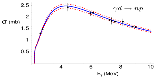
Figure 2: The photodissociation cross section for $\gamma+d\rightarrow n+p$ as a function of energy with counterterm $L_{1}$ determined via the threshold capture cross section for $n+p\rightarrow d+\gamma$. The dashed lines indicate the theoretical uncertainty.

4 Calibrating the Sun

Another application of EFT methods is in weak interactions. The mechanism by which stars—especially our sun—generate their prodigious energy has long been of interest to physicists. First proposed at the end of the 1930’s by Bethe and Critchfield, the basic process is summarized via

$$4p\rightarrow{}^{4}He+2e^{+}+2\nu_{e}+25\,\,{\rm MeV}$$ (23)

while the detailed reaction picture is shown in Figure 1. However, despite the fact that this hypothesis has been around now for over six decades, it is only recently, with the advent of large scale neutrino detectors, that direct tests of this picture have become possible. As is well-known, such tests have in general revealed a deficit of such neutrinos and this problem has given rise to the suggestion of neutrino oscillations, which has become a field unto itself[21]. Implicit in this observation is the assumption that the rate for the reaction

$$p+p\rightarrow d+e^{+}+\nu_{e}$$ (24)

which begins this chain is correctly calculated. A theoretical evaluation is required here since the only experimental measurement—

$$\sigma(\nu_{e}+d\rightarrow p+p+e^{-})_{exp}=(53\pm 18)\times 10^{-42}\,\,{\rm cm}^{2}$$ (25)

by LAMPF E31[22]—while in agreement with the corresponding theoretically calculated value[23]

$$\sigma(\nu_{e}+d\rightarrow p+p+e^{-})_{th}=52\times 10^{-42}\,\,{\rm cm}^{2},$$ (26)

has only $\sim 35\%$ precision.

On the theoretical side, calculation of the reaction Eq. 24 consists of two components:

• convolution of the one-body operator, obtained from neutron beta decay, with the deuteron and pp wavefunctions;

• evaluation of the two-body piece, which is generally described via a meson-exchange approach.

The first part is reasonably secure, which cannot be said for the two-body part of the calculation. This is evidenced by the fact that two such calculations of total cross sections for the related reaction

$$\nu_{x}+d\rightarrow n+p+\nu_{x}$$ (27)

by Ying, Haxton, and Henley (YHH)[24] and by Kubodera and Nozawa 2(KN) [23] differ by $\sim 5\%$, as shown in Figure 3. YHH included exchange currents only to the extent that they are incorporate through the constraints of current conservation, imposed by a generalized Siegert’s theorem. KN included in addition model-dependent contributions of exchange currents.

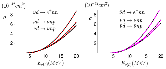
Figure 3: Inelastic $\nu(\bar{\nu})d$ cross sections vs. incident $\nu(\bar{\nu})$ energy. The solid curves in the left hand figure are the results of Kubodera and Nozawa, while the dot-dashed curves, which sit on top of the solid curves are NLO in EFT with $L_{1,A}$=6.3 fm³. The results given in the right hand graph are those of Ying, Haxton, and Henley, with the dashed curves which lie on top generated at NLO in EFT with $L_{1,A}$=1.0 fm³.

There has been recent work in which model-dependence of the exchange currents, arising primarily from poorly known couplings involving N-$\delta$ transitions, has been reduced by appealing to the known $\beta$ decay rate of the similar Gamow-Teller transition in ³He. This, of course, does not entirely circumvent the problem because three-body nuclear forces are then entangled in the analysis, and because a specific model-dependent set of exchange current diagrams are considered. The YHH and KN calculations are both fairly traditional nuclear physics calculations, and the resulting differences are probably a fair estimate of the uncertainties arising from the choice of nuclear potential and the description of exchange current and other short-range effects. While such discrepancies are perhaps not important for some applications, in the case of the reaction Eq. 24, which initiates the solar burning chain, and Eq. 27, which is used as a signal for neutrino-initiated neutral current reactions at the SNO detector, such a considerable uncertainty is unacceptable.

The methods of effective field theory can be used to resolve the problem. The inputs required for such calculations are simply the neutron decay axial decay constant $g_{A}$ and the experimental value of the deuteron binding energy, together with the experimental $np,\,pp$ scattering lengths and effective ranges. Since this is a low energy reaction the rescattering corrections which renormalize the basic decay process can be reliably included, and such calculations for the charged and neutral current neutrino reactions have recently been done by Butler and Chen[26]. A parallel and related calculation for the reaction Eq. 24 has been performed by Kong and Ravndal[27].

In both evaluations, however, there exists the same unknown quantity—a four-nucleon axial current counterterm of the form

$$\vec{A}^{(2)}={1\over 8}L_{1A}(N^{T}\sigma_{2}\vec{\sigma}\tau_{2}N)^{\dagger}(N^{T}\sigma_{2}\tau_{2}\tau_{-}N)$$ (28)

where $L_{1A}$ has units of fm³ and is expected by is by EFT scaling arguments to be in the range $-6\,\,{\rm fm}^{3}\leq L_{1A}\leq+6\,\,{\rm fm}^{3}$, corresponding to a cross section difference of $\sim 10\%$. In fact, Butler and Chen have shown that the calculations of YNN and KN can be completely characterized via the values

$$L_{1A}=\left\{\begin{array}[]{cc}6.3\,\,{\rm fm}^{3}&YHH\cite[cite]{[\@@bibref{}{yhh}{}{}]}\\ 1.0\,\,{\rm fm}^{3}&KN\cite[cite]{[\@@bibref{}{kn}{}{}]}\end{array}\right.$$ (29)

This large difference for values of $L_{1A}$ simply corresponds to differing assumptions about the short-range properties of the nucleon-nucleon interaction associated with the meson-exchange calculations.

Obviously, one can generate alternative values of $L_{1A}$ via other descriptions of short-range structure, but it is clear that the best approach would be to measure this counterterm experimentally, say via the charged current reaction

$$\nu_{e}+d\rightarrow p+p+e^{-}$$ (30)

The corresponding experimental value of the counterterm could then be used to yield a theoretically rigorous $\sim 2\%$ prediction for the reaction rate for the pp neutrino process which initiates the solar burning cycle and for the neutral current deuteron disintegration reaction Eq. 27 which is used in the SNO detector in order to indicate that a neutral current neutrino reaction has occurred. Finally, it is clear that careful measurement to pin down the size of the counterterm $L_{1A}$ would offer a target for theorists to shoot at in order to gauge their models of short distance NN structure.

5 Conclusions

We have tried to give a didactic introduction to effective field theory methods in a variety of applications. In each case we have generated an effective interaction which is valid in a given (usually low energy) range. In the case of Rayleight scattering the EFT procedure was found to reveal the physics of the process in a simple fashion. In the case of low energy QCD, chiral perturbation theory was able to elicit reliable predictions in an otherwise intractable energy region. In the case of the NN interaction we have seen how the use of EFT methods allows model-independent predictions for low energy weak and electromagnetic processes to be made once low energy counterterms are determined theoretically. Space limitations do not allow us to give further examples, but work is underway in a number of areas. One is the extension to systems with three or more constituents. In this case, Bedaque, Hammer, and van Kolck have shown how the $nd$ scattering length in the quartet channel $a_{3\over 2}^{exp}=6.35\pm 0.02$ fm can be predicted in terms of known NN quantities, yielding $a_{3\over 2}^{eft}=6.32\pm 0.1$ fm[28]. However, things are more difficult in the doublet case. Efforts are also underway to simplify large basis shell model calculations using EFT methods. Another challenge is how to extend such techniques to higher energy. Here the counting scheme which should work, PDS wherein pion exchange is treated perturbatively, seems to have convergence difficulties[30], while that which is less on firm ground—Weinberg power counting—seems to give reasonable results[31]. There is still much to do!

Acknowledgement

It is a pleasure to acknowledge the hospitality of the organizers of this Few Body meeting. This work was supported in part by the National Science Foundation.

References

- [1] B.R. Holstein, Am. J. Phys. 67, 422 (1999).
- [2] A corresponding classical physics discussion is given in R.P Feynman, R.B. Leighton, and M. Sands, The Feynman Lecures on Physics, Addison-Wesley, Reading, MA, (1963) Vol. I, Ch. 32.
- [3] See, e.g. A. Manohar, ”Effective Field Theories,” in Schladming 1966: Perturbative and Nonperturbative Aspects of Quantum Field Theory, hep-ph/9606222; D. Kaplan, ”Effective Field Theories,” in Proc. 7th Summer School in Nuclear Physics, nucl-th/9506035,; H. Georgi, ”Effective Field Theory,” in Ann. Rev. Nucl Sci. 43, 209 (1995).
- [4] S. Gasiorowicz and D.A. Geffen, Rev. Mod. Phys. 41, 531 (1969).
- [5] M. Gell-Mann, CalTech Rept. CTSL-20 (1961); S. Okubo, Prog. Theo. Phys. 27 (1962) 949.
- [6] S. Weinberg, Physica A96 (1979) 327.
- [7] J. Gasser and H. Leutwyler, Ann. Phys. (NY), 158, 142 (1984); Nucl. Phys. B250, 465 (1985).
- [8] A. Manohar and H. Georgi, Nucl. Phys. B234 (1984) 189; J.F. Donoghue, E. Golowich and B.R. Holstein, Phys. Rev. D30 (1984) 587.
- [9] See, e.g., B.R. Holstein, Int. J. Mod. Phys. A7, 7873 (1992).
- [10] Particle Data Group, Phys. Rev. D54, 1 (1996).
- [11] Yu. M. Antipov et al., Z. LPhys. C26, 495 (1985).
- [12] Yu. M. Antipov et al., Phys. Lett. B121, 445 (1983).
- [13] T.A. Aibergenov et al., Czech. J. Phys. 36, 948 (1986).
- [14] D. Babusci et al., Phys. Lett. B277, 158 (1992).
- [15] J. Gasser, M. Sainio, and A. Svarc, Nucl. Phys. B307, 779 (1988).
- [16] V. Bernard, N. Kaiser, and U.G. Meissner, Int. J. Mod. Phys. E4, 193 (1995).
- [17] J.-W. Chen, G. Rupak, and M.J. Savage, Nucl. Phys. A653, 386 (1999).
- [18] M.J. Savage, K.A. Scaldeferri, and M.B. Wise, Nucl. Phys. A652, 273 (1999).
- [19] D.O. Riska and G.E. Brown, Phys. Lett. B38, 193 (1972).
- [20] G. Rupak, nucl-th/9911018
- [21] See, e.g. W.C. Haxton and B.R. Holstein, Am. J. Phys. 68, 15 (2000).
- [22] S.E. Willis et al., Phys. Rev. Lett. D4, 522 (1980).
- [23] K.Kubodera, and S. Nozawa, Int. J. Mod. Phys. E3, 101 (1994) and USC(NT)-Report-92-1, 1992, unpublished. 1030 (1988); see also S. Nakamura, T. Sata, V.. Gudkov, and K. Kubodera, nucl-th/0009012.
- [24] S. Ying, W. Haxton, and E. Henley, Phys. Rev. D40, 3211 (1989) and Phys. Rev. C45, 1982 (1992).
- [25] See, e.g. D.B. Kaplan, M.J. Savage, and M.B. Wise, Phys. Lett. B424, 390 (1998); Nucl. Phys. B534, 329 (1998).
- [26] M. Butler and J. Chen, Nucl. Phys. A675, 575 (2000).
- [27] X. Kong and F. Ranvdal, nucl-th/0004038.
- [28] P.F. Bedaque, H.W. Hammer, and U. von Kolck, Nucl. Phys. A646, 444 (1999); see also B. Blankleider and G. Gegelia, nucl-th/0009007.
- [29] W.C. Haxton and C. L. Song, nucl-th/9907097 and nucl-th/9908082.
- [30] D.B. Kaplan, M.J. Savage, and M.B. Wise, Phys. Lett. B424, 390 (1998); Nucl. Phys. B534, 329 (1998).
- [31] S. Weinberg, Phys. Lett. B251, 288 (1990); Nucl. Phys. B363, 3 (1991); Phys. Lett. B295, 114 (1992).