Two-neutron separation energies, binding energies and phase transitions in the interacting boson model

Abstract

In the framework of the interacting boson model the three transitional regions (rotational-vibrational, rotational–$\gamma$-unstable and, vibrational–$\gamma$-unstable transitions) are reanalyzed. A new kind of plot is presented for studying phase transitions in finite systems such as atomic nuclei. The importance of analyzing binding energies and not only energy spectra and electromagnetic transitions, describing transitional regions is emphasized. We finally discuss a number of realistic examples.

PACS numbers: 21.60-n, 21.60Fw, 21.60Ev

I Introduction

In the last few years, interest for the study of phase transitions and phase coexistence in atomic nuclei has been revived [1, 2, 3, 4] in particular making use of the Interacting Boson Model (IBM) [5]. In the chart of nuclei, three transitional regions can be distinguished where one observes rapid structural changes: (a) In the Nd-Sm-Gd region, one observes a change from spherical to well-deformed nuclei when moving from the lighter to the heavier isotopes; in the IBM language this is the $U(5)$-$SU(3)$ transitional region; (b) in the Ru-Pd region, one notices that the lighter isotopes are spherical while the heavier ones indicate a $\gamma$-unstable character, this is the $U(5)$-$O(6)$ region; (c) in the Os-Pt region, the lighter isotopes are well deformed while the heavier shown $\gamma$-unstable properties, this is the $SU(3)$-$O(6)$ transitional region. Although these three transitional regions have been studied extensively in the framework of the IBM [6, 7, 8, 9] (note that in this paper we use the simplest version of the model, IBM-1, therefore we do not consider the transitional regions using IBM-2 [7, 10, 11]), the discussion of phase transitions has not always been treated in a proper way. In particular one of the weak points is how to define an appropriate control parameter in a system such as the atomic nucleus where this parameter is fixed (for given $N$ and $Z$) and cannot be controlled externally [12]. This problem has been recently considered in a study by Casten et al.  [3].

Binding energy (BE) serves as an appropriate “signature” for phase transitions in nuclei [12, 13]. The binding energy of the nucleus or, equivalently its mass, is one of the more important nuclear properties to be determined. In some cases this is the only knowledge about a nucleus when situated far from stability. In the last few years, the development of new experimental facilities has given access to very unstable nuclei and many new mass measurements have been obtained [14]. In the light of the variety of nuclear properties (nuclear mass, nuclear moments, $\ldots$) that have been obtained recently, a theoretical study concentrating on the nuclear binding energy and, related to that, possible phase transition is desirable.

Binding energies contain important information about nuclear structure. In IBM calculations, only spectra and electromagnetic transitions used to be analyzed and the description of the binding energy is in most of the cases excluded. In the present article we show that it is convenient to explore nuclear binding energies in order to obtain a consistent description, especially when one is dealing with chains of isotopes. It must be noted that the study of binding energies can help to discriminate between apparently equivalent descriptions of energy spectra and electromagnetic transitions rates for a given nucleus or, even for a chain of nuclei.

In section II we review the study of phase transitions in the IBM. In section III a new way of dealing with phase transitions in nuclei will be presented together with the study of two-neutron separation energies (S_2n) in regions where phase transition might happen. In section IV we study some realistic cases and, finally, in section V, we present our conclusions.

II Transitional regions and phase transitions in the IBM: a study of nuclear binding energies

The IBM is an algebraic model able to describe the low-lying collective states in even-even nuclei in terms of bosons which carry either angular momentum $L=0$ ($s$ bosons) or angular momentum $L=2$ ($d$ bosons) [5]. The system of bosons, for which the number of bosons equals half the number of valence fermions, $N=n/2$, interacts through a Hamiltonian that typically includes up to two-body interactions, is number conserving and rotationally invariant. The original version of the model, the IBM-1, is used in the present article.

The IBM has been extensively used during the last decades for the study of medium and heavy nuclei [15]. One of the main challenges for the model was the description of transitional regions, where the structure of the nuclei can change rapidly along a chain of isotopes. In particular, different transitional regions have been obtained where such changes in the nuclear structure appear: from spherical to well deformed nuclei (Nd, Sm, and Gd region), from well deformed to $\gamma$-unstable nuclei (Ru and Pd region) or from spherical to $\gamma$-unstable (Os and Pt region). In the IBM language a spherical nucleus is related to the $U(5)$ limit, a well deformed nucleus is related to the $SU(3)$ limit, while $\gamma$-unstable nuclei correspond to the $O(6)$ limit. A compact Hamiltonian for analyzing the three previous regions can be depicted as follows,

$$\hat{H}=\kappa\Big{(}N{1-\xi\over\xi}\hat{n}_{d}-\hat{Q}\cdot\hat{Q}\Big{)}+\kappa^{\prime}\hat{L}\cdot\hat{L},$$ (1)

with $0\leq\xi\leq 1$. The coefficient of the one-body term can be rewritten as $N(1-\xi)/\xi=\epsilon_{d}/\kappa$, where $\epsilon_{d}$ is the single-particle energy for the $d$ bosons. On the other hand, $\hat{n}_{d}$ is the $d$ boson number operator and

$$\hat{L} = \sqrt{10}(d^{\dagger}\times\tilde{d})^{(1)},$$ (2)

$$\hat{Q} = s^{\dagger}\tilde{d}+d^{\dagger}\tilde{s}+\chi(d^{\dagger}\times\tilde{d})^{(2)}.$$ (3)

The symbol $\cdot$ represents the scalar product. In this work the scalar product of two operators with angular momentum $L$ is defined as $\hat{T}_{L}\cdot\hat{T}_{L}=\sum_{M}(-1)^{M}\hat{T}_{LM}\hat{T}_{L-M}$ where $\hat{T}_{LM}$ corresponds to the $M$ component of the operator $\hat{T}_{L}$. The operator $\tilde{\gamma}_{\ell m}=(-1)^{m}\gamma_{\ell-m}$ (where $\gamma$ refers to $s$ and $d$ bosons) is introduced to ensure the tensorial character under spatial rotations. With this Hamiltonian one can explore the three transitional regions which correspond to the segments of the symmetry triangle [16].

One of the most striking facts that happen in the transitional regions is the possibility of observation of phase transitions. A phase transition can roughly be defined as a qualitative change in a given property of a system. In order to characterize the properties of the system one has to introduce an order parameter. Another important concept is the order of a transition which is the degree of the derivative for a given experimental observable which first experiences a discontinuity. In the atomic nucleus this experimental observable is the binding energy or, the related two-neutron separation energy (S_2n). Although phase transitions are strictly well defined in macroscopic systems and the atomic nucleus is a finite system, a number of studies have shown that the concept of a phase transition retains its validity and usefulness in small systems too [17, 18, 13, 19]. A very useful tool in order to discuss phase transitions in finite system are the coherent states which, in the case of the IBM, are also known as intrinsic states [20, 12, 21]. The intrinsic-state formalism provides a connection between the IBM and the Geometrical Collective Model [22]. The key point for establishing this connection is to consider that the dynamical behavior of the system can be described, to a first approximation, as arising from independent bosons moving in an average field [23]. The ground state of the system is a condensate, $|c\rangle$, of bosons that occupy the lowest-energy phonon state $\Gamma^{\dagger}_{c}$,

$$|c\rangle={1\over\sqrt{N!}}(\Gamma^{\dagger}_{c})^{N}|0\rangle,$$ (4)

where

$$\Gamma^{\dagger}_{c}={1\over\sqrt{1+\beta^{2}}}\left(s^{\dagger}+\beta\cos\gamma\,d^{\dagger}_{0}+{1\over\sqrt{2}}\beta\sin\gamma\,(d^{\dagger}_{2}+d^{\dagger}_{-2})\right).$$ (5)

Here, the variables $\beta$ and $\gamma$, that are obtained after minimization of the ground-state energy, are the order parameters of the system. A spherical nucleus will have as order parameters $\beta=0$ and an arbitrary value for $\gamma$; a deformed nucleus is characterized by a finite value of $\beta$ (in the $SU(3)$ limit for $N\rightarrow\infty$ one has $\beta=\sqrt{2}$) and $\gamma=0$ (prolate nucleus) or $\gamma=\pi/3$ (oblate nucleus); and a $\gamma$-unstable nucleus corresponds to $\beta=1$ (in the limit $N\rightarrow\infty$) and to an arbitrary value for $\gamma$. A phase transition will produce changes in the order parameter of the system. Using the intrinsic state we get “microscopic” information on the order parameter.

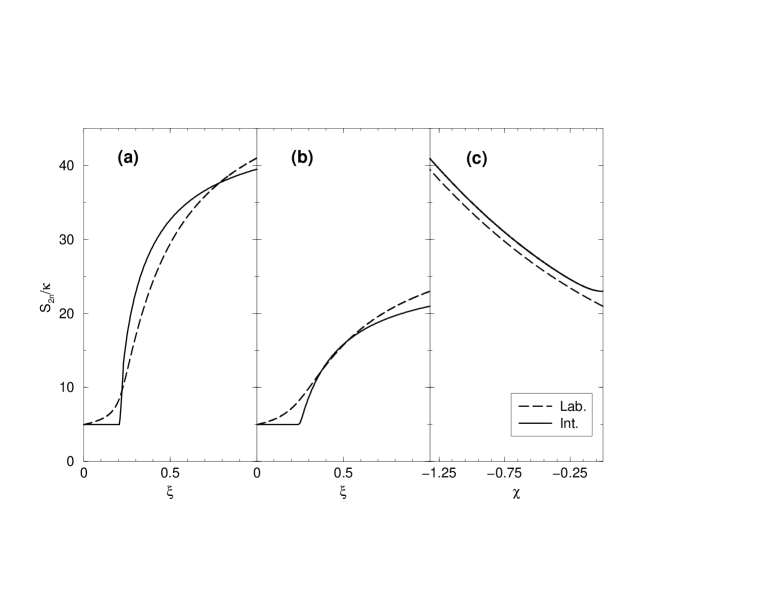
First, we analyze the behavior of the binding energy and two-neutron separation energy in the three transitional regions. In the three cases the results are independent of the value of $\kappa^{\prime}$ in eq. (1). For the $U(5)$-$SU(3)$ transition the value of $\xi$ varies from $0$ ($U(5)$) to $1$ ($SU(3)$) with $\chi=\pm\sqrt{7}/2$ [16]; in the $U(5)$-$O(6)$ transition the value of $\xi$ varies from $0$ ($U(5)$) to $1$ ($O(6)$) with $\chi=0$ [16]; finally in the transition $SU(3)$-$O(6)$ the value of $\chi$ varies from $\pm\sqrt{7}/2$ ($SU(3)$) to $0$ ($O(6)$) with $\xi=1$ [16]. In figures 1a, 1b, and 1c we present the binding energy in the laboratory system and in the intrinsic frame ($BE/\kappa$) while in figures 1a’, 1b’, and 1c’ we present the value of $\beta$ in the three transitional regions for a number of bosons $N=10$. First of all, it must be emphasized that the binding energy calculated in the intrinsic system is always below the exact value because it derives from a variational method. One can also realize that the intrinsic-state calculations show a sharp behavior in the phase transition regions while the diagonalization in the laboratory frame leads to smooth curves. In this sense the variational procedure mimics very well what happens in the thermodynamic limit. One of the characteristics of phase transitions in macroscopic systems is that they are very sharp, but in finite system the sharpness will depend on the number of particles.

In figure 1a, a first order transition shows up (discontinuity in the slope of the BE), and also a discontinuity in the value of the order parameter exits. In figure 1b, a phase transition also appears, but in this case it is a second-order transition (discontinuity in the curvature of the BE). One observes, more generally, that there exits a line of first order transitions for Hamiltonians with $\chi\neq 0$ and just one point for a second-order transition in the case of $\chi=0$ [5]. The parametrization of the Hamiltonian (1) is very appropriate because the phase transition appears approximately at the same value of the control parameter ($\xi$) for any value of $N$ [4]. This critical point, $\xi_{c}$, can be obtained easily from the expression for the energy given in [24] as

$$\xi_{c}={N\over 5N+\chi^{2}-8}.$$ (6)

For $\xi<\xi_{c}$ the potential has a local minimum in $\beta=0$, while for $\xi>\xi_{c}$ this local minimum becomes a local maximum. It is clear from this expression that for a large number of bosons, $\xi_{c}\approx 0.2$. Finally, in figure 1c no phase transition appears and both calculations, exact diagonalization and intrinsic-state, lead to a smooth transitions.

In a next step, we analyze the behavior of the two-neutron separation energy. The definition that will be used along this paper is,

$$S_{2n}(N)=BE(N)-BE(N-1).$$ (7)

In the calculation of S_2n two different nuclei are involved, which makes necessary to impose an assumption in order to relate the Hamiltonians for the nuclei with $N$ and $N-1$ bosons. Here, we consider the simplest (not unrealistic) case which implies the same Hamiltonian in both nuclei. In figure 2 we study the same transitions as in figure 1 and essentially the same remarks hold. Note in this case the crossing of intrinsic-state and laboratory calculations, which is allowed.

So, in this section we have reviewed the study of phase transitions in atomic nuclei, in particular using the IBM, and have shown it is straightforward and clear from a theoretical point of view. In this analysis, however, there is a weak point: the control parameter $\xi$ ($\chi$) is not a genuine one, because it cannot be modified externally. The control parameter only changes when one is moving along a chain of nuclei and also assumes a change in the number of bosons. These two problems have already been remarked and alternative solutions have been proposed [3]. In the next sections, we propose a new strategy for attacking this problem.

III How to identify phase transitions

A The new diagrams “binding energy-number of bosons-control parameter”

A consistent treatment of phase transitions in nuclei must go beyond the study carried out in section II because one has to treat simultaneously the control parameter $\xi$ ($\chi$) and the number of bosons $N$. It must be emphasized that $N$ is not a control parameter because it is a discrete variable and it is fixed in each individual nucleus. Strictly speaking $\xi$ ($\chi$) is neither a genuine control parameter, because its value is also fixed in each given nucleus, nor can it be controlled externally. Only the appropriate interplay of $N$ with $\xi$ ($\chi$) can lead to a proper definition of an order parameter, although with discrete values.

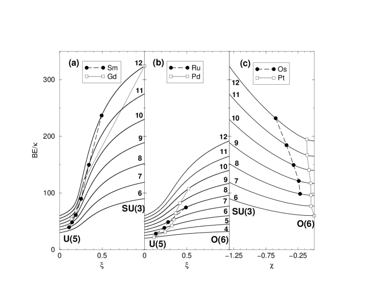
The appropriate way for treating phase transitions and transitional regions is to plot in the same figure the value of the binding energy versus the control parameter and this for different values of $N$. In such a plot, a transition will develop through changes in the control parameter, but at the same time going through curves with a different number of bosons. In order to illustrate this new procedure, we discuss the transitional regions $U(5)$-$SU(3)$, $U(5)$-$O(6)$ and, $SU(3)$-$O(6)$ in figures 3a, 3b, and 3c respectively. In these figures, only the laboratory results (IBM diagonalization) are presented. As an example, trajectories for real nuclei are also plotted in each figure. A procedure in order to obtain the value of the control parameter, for each nucleus, will be explained in section IV. The more interesting cases appear in figures 3a and 3b because there, phase transitions indeed happen. So, looking at these figures, one can easily see if a given nucleus is situated in the spherical region ($\xi$ near to $0$), in the deformed region ($\xi$ around 1) or at the critical point.

One might be tempted to consider similar plots for the two-neutron separation energies. In this case one must be very careful because the Hamiltonian for $N$ and $N-1$ bosons are different. That means that S_2n is not a function of a single control parameter, $\xi$ ($\chi$), anymore, but becomes a function of two control parameters, one for $N$ and another one for $N-1$.

The essential difference between phase transitions in nuclei compared to macroscopic systems is the existence of a control parameter in the macroscopic case, such as temperature or pressure, that can be controlled externally. In the case of atomic nuclei, the only way for changing the value of the control parameter is to move along a chain of nuclei. It is clear that the variation of the control parameter is thereby fixed and cannot be modified externally.

B Crossing the phase transition region: anomalies in the two-neutron separation energies

In previous sections we have studied the behavior of the binding energy as a function of the control parameter, i.e. as a function of the Hamiltonian, in the three transitional regions of the IBM. Due to the specific characteristics of phase transitions in atomic nuclei, it is not a priori clear how different observables will behave when crossing a critical value through a chain of isotopes. More particular, one can observe the two-neutron separation energies as a function of the nucleus in the chain that one considers. S_2n is indeed a very appropriate observable to be analyzed because it contains important information about the nuclear structure, in particular on the ground state.

Before starting the present analysis we emphasize the fact that there exits an extra contribution to the binding energy not yet included when using the Hamiltonian of equation (1), i.e. 

$$E^{\prime}=E_{0}+AN+{B\over 2}N(N-1)$$ (8)

Those extra terms, deriving from the linear and quadratic $U(6)$ Casimir invariant, take into account the bulk contribution of the nuclear interaction. Including those extra terms in S_2n, one obtains a linear contribution to be added to the IBM calculation, resulting

$$S_{2n}(N)=(A-B/2)+BN+BE_{IBM}(N)-BE_{IBM}(N-1).$$ (9)

When the linear dependence is excluded from S_2n, we will refer to that result as S’_2n. It must be noted that the specific nuclear structure IBM contribution in the three dynamical limits ($U(5)$, $SU(3)$, and $O(6)$) is also linear in the boson number [5, 25] and in this context only a particular change in the internal structure of the nuclei, as happens during the phase transitions, can perturb this linear dependence.

In order to be sure one encounters a phase transition or passes through a specific transitional region, one has to establish the value of the control parameter for each nucleus. In the following we will concentrate on chains of isotopes (fixed number of protons), being the nuclei characterized by a given number of bosons $N$ or by the number of neutron pairs $N_{\nu}$. As a consequence one has to determine the functional relation $\xi=\xi(N)$ ($\chi=\chi(N)$) or, in terms of the number of neutron pairs, the relation $\xi=\xi(N_{\nu})$ ($\chi=\chi(N_{\nu})$). Although the latter functional relation must be determined from experimental data, one can use a simple function and see if it is possible to obtain some physical insight on the structure of S_2n. For the present study we fix a chain of isotopes with $5$ protons pairs, $N_{\pi}=5$, and a variable number of neutrons pairs, ranging from $N_{\nu}=0$ to $N_{\nu}=10$. Two functional dependences will be used, firstly linear and secondly quadratic. Next, we show the different parametrizations for the different transition regions,

• $U(5)$-$SU(3)$ and $U(5)$-$O(6)$ transitional regions.

  $$\xi = 0.099N_{\nu}+0.01,$$ (10)

  $$\xi = 0.0099N_{\nu}^{2}+0.01,$$ (11)

• $SU(3)$-$O(6)$ transitional region.

  $$\chi = -{\sqrt{7}\over 20}N_{\nu}$$ (12)

  $$\chi = -{\sqrt{7}\over 200}N_{\nu}^{2}.$$ (13)

Using parametrizations (10,11), $\xi$ ranges from $0.01$ to $1$. On the other hand, using parametrization (12,13), $\chi$ ranges from $0$ to $-\sqrt{7}/2$. In order to establish a realistic parametrization, we start from the empirical observation that in the $U(5)$-$SU(3)$ transition, the system passes from the $U(5)$ to the $SU(3)$ limit when the number of bosons is increasing [15]. Similarly, the transition $U(5)$-$O(6)$ implies that the system goes from $U(5)$ to $O(6)$ when the number of bosons is increasing. Finally, the transition $SU(3)$-$O(6)$ implies the system passes from $SU(3)$ to $O(6)$ when the number of bosons is decreasing.

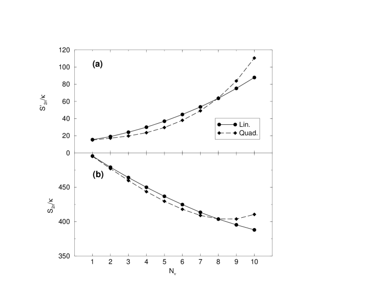
In figures 4a and 4b, S_2n and S’_2n are shown, respectively, for the $U(5)$-$SU(3)$ transitional region using for $\xi$ the parametrizations (10,11). The Hamiltonian (1) has been used with $\chi=-\sqrt{7}/2$ [16]. For convenience, a linear dependence equal to $S_{2n}^{lin}/\kappa=200-20N_{\nu}$ has been chosen as a reference value in order to obtain a realistic behavior in S_2n. In these figures, an anomaly in the linear dependence of S_2n and S’_2n, right at the place where the phase transition happens, can be appreciated. The phase transition point corresponds approximately to $\xi\approx 0.2$ (see figure 1a and 1a’) and taking into account equations (10) and (11) results a value for $N_{\nu}$, $N_{\nu}\approx 2$ and $N_{\nu}\approx 4$ for the linear and quadratic dependence, respectively. We point out that in case a quadratic variation in $N_{\nu}$ for the control parameter is selected, the anomaly in S_2n is more pronounced than for a linear variation. In figures 5a and 5b, S_2n and S’_2n are shown, respectively, for the $U(5)$-$O(6)$ transitional region using for $\xi$ the same parametrization as in the previous case. The Hamiltonian (1) has been used with $\chi=0$ [16]. In this case a linear dependence equal to $S_{2n}^{lin}/\kappa=200-10N_{\nu}$ has been used to determine the S_2n values. Again, a non-linear behavior appears at the point of the phase transition. The phase transition point corresponds approximately to $\xi\approx 0.2$ (see figure 1b and 1b’) and taking into account equations (12) and (13) results a value for $N_{\nu}$, $N_{\nu}\approx 2$ and $N_{\nu}\approx 4$ for the linear and quadratic dependence, respectively. In this case, a linear variation in the control parameter leads to an almost linear dependence in S_2n and S’_2n. Only a control parameter which depends quadratically on $N_{\nu}$ produces a kink in the two-neutron separation energy. Finally, in figures 6a and 6b, S_2n and S’_2n are represented, respectively, for the $SU(3)$-$O(6)$ transitional region using for $\chi$ the parametrizations (12,13). The Hamiltonian (1) has been used with $\xi=1$ [16]. In this case the following linear dependence $S_{2n}^{lin}/\kappa=200-20N_{\nu}$ has been chosen as a reference when calculating S_2n. In this transitional region no phase transition is observed and a smooth curvature result except when one is approaching the $SU(3)$ limit and is using a quadratic dependence in $N_{\nu}$ for $\chi$ (13).

Along this section we have learned to treat in a proper way binding energies (two-neutron separation energies) in transitional regions where phase transitions might appear. We have seen that in these regions one can get deviations from the linear tendency of S_2n. Next step will be to find experimental examples where those anomalies appear and explain them using the IBM.

IV Realistic calculations

Within the framework of the IBM, the energy spectra and transition rates of many medium-mass and heavy nuclei have been analyzed very successfully. However, in most of these studies [15] the binding energies have been ignored. One of the reasons for such a neglect stems (partly) from the fact that the early IBM studies (carried out in the 80’s) [7, 10, 11] gave a rather good reproduction of the general trends of the nuclear binding energy in different mass regions. So, it was tacitly assumed that realistic IBM calculations would also reproduce (in a natural way) the binding energy values. In the mean time, with a large increase in the precision for the mass measurement [27, 28, 14], much improved data have been established [29]. Moreover, it must be noted that, in order to carry out a proper comparison between calculated and experimental binding energies (or $S_{2n}$ data), one cannot concentrate on single or a few nuclei. Large chain of isotopes have to be considered and this complicates considerably performing consistent IBM calculations.

In this section we will determine the experimental relations between the control parameter $\xi$ ($\chi$) and the number of neutron pairs $N_{\nu}$ through explicit fits of energy spectra for selected nuclei in the three transitional regions. Starting from these relations we are able to represent a specific chain of isotopes on the diagrams shown in section III A. We subsequently show that the experimental binding energies (or two-neutron separation energies) are not always well reproduced although the spectra do. We analyze chains of isotopes in the transitional regions (i) first using the more standard set of parameters for the Hamiltonian [5] and (ii), secondly, we compare with an alternative parametrization (see discussion below). We do not aim a perfect fit of the experimental data, but we intend to emphasize the influence of choosing various parametrizations on the binding energies.

Next we study the three transitional regions:

• The $U(5)$-$SU(3)$ transitional region

  There exit nuclei that exhibit a drastic change in the internal structure when one is passing their isotopes series, going from a vibrational into a rotational behavior. Typical examples are situated in the rare-earth region, such as the Nd, Sm, and Gd nuclei. The Sm nuclei have been extensively studied in Ref. [6] and a very good agreement with experimental data for S_2n has been obtained. In figure 3a, we plot the position of the different Sm isotopes and one can clearly see how they cross the critical point, in particular ¹⁵²Sm is situated almost exactly where the phase transition happens. The cases of Nd and Gd are very similar. Here, we will only focus to the case of Gd.

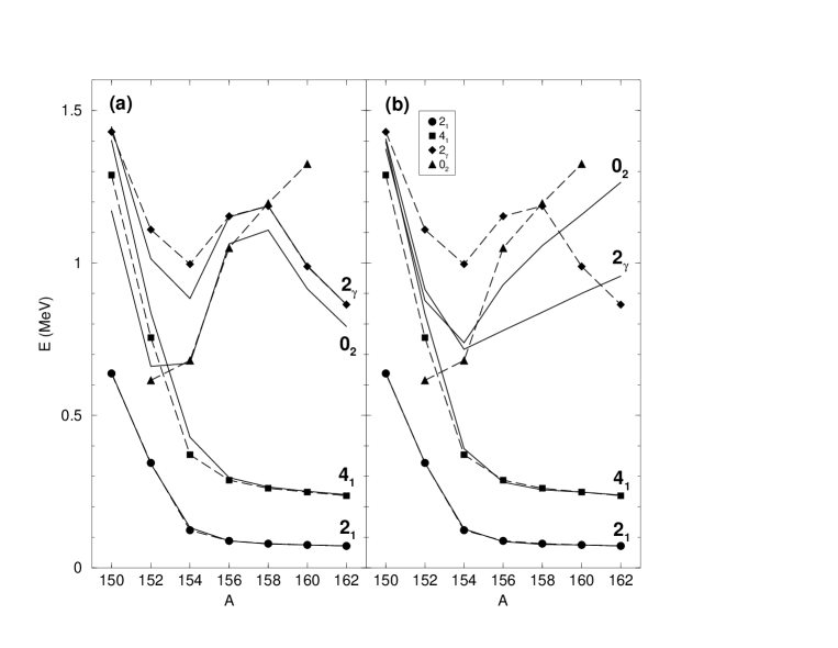
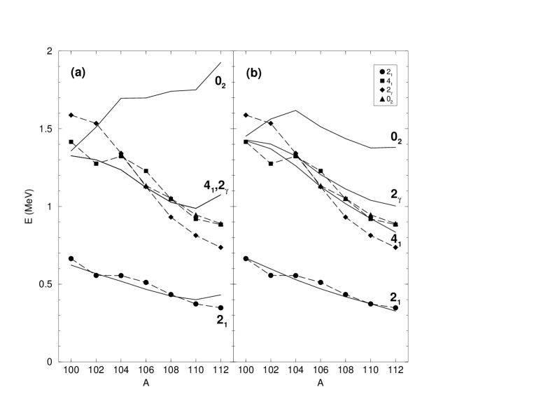
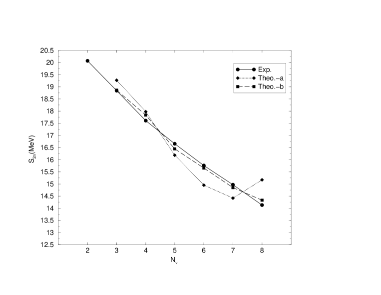
  In this region we assume a value $\chi=-\sqrt{7}/2$ because some Gd isotopes clearly exhibit the character of the $SU(3)$ dynamical symmetry [5]. This assumption was very successful in describing the Sm nuclei, which form neighboring nuclei. With this ansatz we have carried out a fit to the energy spectra of the Gd isotopes (from ¹⁵⁰Gd until ¹⁶²Gd) using the Hamiltonian (1). In order to obtain the parameters, we tried to reproduce the rotational structure of the ground- and $\gamma$-band as well as possible. The ¹⁵⁰Gd nucleus still shows a vibrational structure while ^156-162Gd are considered as rather good $SU(3)$ examples. The parameters for ¹⁵⁰Gd to ¹⁶²Gd, respectively, are shown in table I (upper part). In figure 7a we compare the theoretical and the experimental energies for the low-lying levels using this set of parameters. Those values are used to position the Gd isotopes in the phase transition diagram of figure 3a, where ¹⁵⁰Gd corresponds to $N=9$ while ¹⁵⁶Gd corresponds to $N=12$. Note that ^158-162Gd are not plotted; they also corresponds to $\xi=1$. From figure 3a one can observe a sudden transition in the Gd isotopes from a vibrational regime into the $SU(3)$ limit. Up to now, we have obtained a good description of the Gd energy spectra but we have to consider the experimental two-neutron separation energies too. This comparison is carried out in figure 8 (the present calculation corresponds to Theo.-a), using a linear contribution $S^{lin}_{2n}=15-0.252N_{\nu}$ (MeV) as a background. One observes a very bad agreement which points to the fact that the use of $\chi=-\sqrt{7}/2$ is not appropriate. A different approach to fix the Hamiltonian is proposed in [26]. There, it is assumed that in well deformed nuclei one can keep the value of $\kappa$ constant around $\kappa=30$ keV and smoothly change the values of $\chi$ and $\epsilon_{d}$ along a series of isotopes. In the present case, the appropriate values for $\chi$ and $\kappa$ are $\chi=-0.6$ and $\kappa=19.2$ keV. On the other hand the values of $\xi$ (using $N(1-\xi)/\xi=\epsilon_{d}/\kappa$, see equation (1)) are shown in table I (lower part) in going on ¹⁴⁶Gd until ¹⁶²Gd (note that in this case, a few extra isotopes are also considered). In figure 7b we again compare the theoretical and the experimental energies for the low-lying levels corresponding to the new Hamiltonian. Again, we compare the calculated S_2n values with the data and, as can be seen in figure 8 (this calculation corresponds to Theo.-b), using a linear contribution $S^{lin}_{2n}=16.75-0.607N_{\nu}$ (MeV) as a background, a very good agreement is obtained. Note that the present results for $\xi=\xi(N)$ cannot be represented in figure 3a due to the new value of $\chi$, since figure 3a corresponds to $\chi=-\sqrt{7}/2$. It is worth noting the strong similarities between figure 8 and figure 4b.

• The $U(5)$-$O(6)$ transitional region

  Clear-cut examples of nuclei in which the structure changes from spherical to $\gamma$-unstable are obtained in the Ru and Pd region. Both series of isotopes have already been studied in [8], showing that the lighter isotopes exhibit a vibrational structure while the heavier ones present a $\gamma$-unstable behavior. In reference [8] the general trends have been analyzed but it was shown that difficulties appear when trying to obtain a consistent description for several observables at the same time. Due to the strong similarities between both nuclei, only the study of Pd nuclei will be presented here.

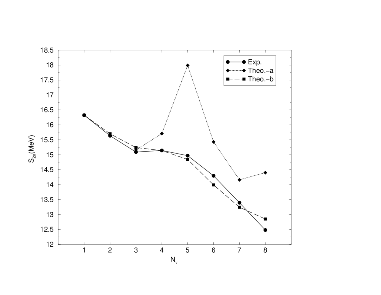
  A first assumption will be to consider $\chi=0$, which is suggested in reference [8] too. Using the Hamiltonian (1) we fit the energy spectra of ^100-112Pd. No other isotopes are fitted because only for those the energy ratio $E(4_{1}^{+})/E(2_{1}^{+})$ changes between $2$ ($U(5)$) and $2.5$ ($O(6)$). Note that this energy ratio will be the main observable to be reproduced during the fits. We have taken a fixed single particle energy at $\epsilon_{d}=65$ keV and the parameters that we have obtained are shown in table II (upper part). Note that no rotational term is necessary. In figure 9a we compare the theoretical and the experimental low-lying levels for this set of parameters. Those values are used to position the Pd isotopes on figure 3b, where ¹⁰⁰Pd corresponds to $N=4$ and ¹¹²Pd corresponds to $N=10$. One can clearly see that the Pd isotopes cover only half the range between the $U(5)$ and the $O(6)$ limit. In figure 10 one obtains a poor description when comparing S_2n (this calculation corresponds to Theo.-a), with a linear contribution $S^{lin}_{2n}=22.27-1.295N_{\nu}$ (MeV) as background, while the energy spectra are well reproduced. Again, this suggests a change in the value of $\chi$. In the following, we will use $\chi=-0.3$, a value that produces a realistic description of the energy spectra. In this case one can fix the single particle energy to $\epsilon_{d}=70$ keV. The obtained values of $(\kappa,\xi)$ from ¹⁰⁰Pd until ¹¹⁴Pd are shown in table II (lower part). In figure 9b we compare again the theoretical and the experimental low-lying levels for the new Hamiltonian. Now, however, one obtains good agreement when comparing experimental and theoretical S_2n values (this calculation corresponds to Theo.-b), with a linear contribution $S^{lin}_{2n}=20.46-0.835N_{\nu}$ (MeV) as a background, as can be seen in figure 10. The new results cannot be represented on figure 3b because $\chi\neq 0$.

• The $SU(3)$-$O(6)$ transitional region

  The most clear-cut examples of nuclei situated in this transitional region are the Os and Pt nuclei. The lighter isotopes exhibit rotational structures while the heavier ones come very close to the $\gamma$-unstable limit. This region has already been studied in [9] in the framework of the IBM-1 but using a different parametrization for the Hamiltonian. Due to the similarities among both series of isotopes, only the analysis of the Pt nuclei will be presented here.

  In order to make a global fit we take into account the fact that ¹⁹⁶Pt is one of the best examples of a $\gamma$-unstable nucleus and, as a consequence, $\chi=0$ and $\xi=0$ [5]. The obtained parameters $(\kappa,\chi,\kappa^{\prime})$ for ¹⁸⁴Pt until ¹⁹⁶Pt are shown in table III (upper part). In figure 11a we compare the theoretical and the experimental low-lying levels for these parameters. If one places these values in figure 3c, where ¹⁹⁶Pt corresponds to $N=6$ while ¹⁸⁴Pt corresponds to $N=12$, it is clear that the Pt isotopes always stay very close to the $O(6)$ limit. Finally, in figure 12, we compare the theoretical and experimental S_2n values (this calculation corresponds to Theo.-a), with a linear contribution $S^{lin}_{2n}=12.66-0.545N_{\nu}$ (MeV) as a background. Again, we obtain a poor agreement in the description of the experimental values. In order to treat this mass region with a slightly different Hamiltonian, one can follow again Ref. [26]. There, it is suggested to include a single-particle energy term. In the case of the Pt nuclei the more appropriate value is $\epsilon_{d}=25.7$ keV. The value of $\kappa$ is also fixed to $\kappa=33.5$ keV and $\kappa^{\prime}=15.2$ keV. The different values of the parameters in the Hamiltonian for ¹⁸⁴Pt until ¹⁹⁶Pt are shown in table III (lower part). In figure 11b we know compare the theoretical and the experimental low-lying levels for the new Hamiltonian. Using this new parametrization, when comparing the S_2n values (this calculation corresponds to Theo.-b), with a linear contribution $S^{lin}_{2n}=11.85-0.649N_{\nu}$ (MeV) as a background, a good agreement is obtained as can be seen in figure 12. These new results cannot be represented in figure 3c because now $\epsilon_{d}\neq 0$.

In this section we have presented two different parameter sets obtained from fitting the energies of the low-lying states of different isotopes of Gd, Pd, and Pt. A very striking fact is, on one side, the good description of the energy spectra for both sets of parameters, and on the other side, the very different results obtained for the two-neutron separation energy using these different parametrizations. The results obtained here were totally unexpected because it was assumed tacitly that a good description of energy spectra would imply a good description for the binding energies too. In order to illustrate this problem, we consider the case of ¹⁴⁸Sm which has been studied by different authors [6, 26]. Although in all the cases the description of the energy spectrum is satisfactory, when calculating the binding energy for the proposed Hamiltonians, one obtains the results $0.939$ MeV (Ref [6]), $1.571$ MeV (Ref [26]) and $2.253$ MeV (also in Ref [26]). All this suggests that a consistent study of atomic nuclei, within the IBM, requires the inclusion of an analysis of the binding energy.

V Summary and conclusions

In the present article, we have analyzed transitional regions and phase transitions in the framework of the IBM. A new kind of diagram (see figure 3) for dealing with phase transitions has been presented. In this diagram we plot the binding energy of the system versus the control parameter (Hamiltonian) for a range in the number of bosons. This procedure turns out to be a particularly convenient method when working in finite systems without a true control parameter.

The main conclusions are twofold:

(i) We have shown that, although the crossing through the phase transition points produces a deviation in the S_2n values from the overall linear background dependence, the way in which, in the given chain of isotopes, this critical point is crossed proves extremely important in deriving clear-cut results. If e.g. the relation between a control parameter and the isotope location (e.g. boson number) is linear, one does not observe dramatic changes in S_2n in any of the three transitional regions ($U(5)$-$SU(3)$, $U(5)$-$O(6)$, and $SU(3)$-$O(6)$). On the contrary, for a quadratic relation, clear changes can appear in the S_2n behavior at the crossing point.

(ii) We have observed that in a consistent study of long chains of isotopes, one has to treat the ground-state (through its binding energy) on equal level with the excited states (relative energy spectrum). It turns out that parameters producing very similar energy spectra can still result in important differences in the ground-state binding energy (order of $1$ MeV).

VI Acknowledgments

The authors are grateful to G. Bollen and co-workers, R.F. Casten, F. Iachello, J. Jolie, P. Van Isacker, and J. Wood for stimulating discussions. The authors like to thank the “FWO-Vlaanderen” for financial support.

FIG. 1.: Binding energies and $\beta$ as a function of the control parameter, in the transitional regions (a) $U(5)$-$SU(3)$, (b) $U(5)$-$O(6)$, and (c) $SU(3)$-$O(6)$. Dashed lines correspond to laboratory calculations while full lines correspond to intrinsic state results. Number of bosons $N=10$.

FIG. 2.: Two-neutron separation energies (S_2n) as a function of the control parameter, in the transitional regions (a) $U(5)$-$SU(3)$, (b) $U(5)$-$O(6)$, and (c) $SU(3)$-$O(6)$. Dashed lines correspond to laboratory calculations while full lines correspond to intrinsic state results. Number of bosons $N=10$.

FIG. 3.: Binding energies in the laboratory system for different numbers of bosons, $N$, as a function of the control parameter, in the transitional regions (a) $U(5)$-$SU(3)$, (b) $U(5)$-$O(6)$, and (c) $SU(3)$-$O(6)$. Full circles and open squares correspond to the theoretical positions of different chains of isotopes.

FIG. 4.: Schematic plot of (a) S_2n and (b) S’_2n in the $U(5)$-$SU(3)$ transitional region. Full lines corresponds to a linear variation of $\xi$ with respect to $N_{\nu}$ while dashed lines corresponds to a quadratic dependence.

FIG. 5.: Schematic plot of (a) S_2n and (b) S’_2n in the $U(5)$-$O(6)$ transitional region. Full lines corresponds to a linear variation of $\xi$ with respect to $N_{\nu}$ while dashed lines corresponds to a quadratic dependence.

FIG. 6.: Schematic plot of (a) S_2n and (b) S’_2n in the $SU(3)$-$O(6)$ transitional region. Full lines corresponds to a linear variation of $\chi$ with respect to $N_{\nu}$ while dashed lines corresponds to a quadratic dependence.

FIG. 7.: Comparison between theoretical and experimental energy levels for Gd isotopes. Full lines correspond to IBM calculations, while symbols connected by dashed lines correspond to experimental data. In panels (a) and (b) different sets of parameters for the IBM calculations are used, see text.

FIG. 8.: Two-neutron separation energies for Gd isotopes. Full lines correspond to experimental data, while dotted and dashed lines correspond to two theoretical calculations, see text.

FIG. 9.: Same caption as in figure 7 but for Pd isotopes.

FIG. 10.: Same caption as in figure 8 but for Pd isotopes.

FIG. 11.: Same caption as in figure 7 but for Pt isotopes.

FIG. 12.: Same caption as in figure 8 but for Pt isotopes.

TABLE I.: Parameters of the Hamiltonian for Gd isotopes ($N_{\pi}=7$). Upper part of the table is referred as Theo.-a and lower part as Theo.-b (as used in the text and in the figures).

Theo.-a $A$ 150 152 154 156 158 160 162 $N_{\nu}$ 2 3 4 5 6 7 8 $\kappa$ 15.4 15.4 15.4 15.4 14.8 11.3 9.1 $\xi$ 0.139 0.192 0.287 1 1 1 1 $\kappa^{\prime}$ 9.0 9.0 9.0 9.0 7.7 8.3 8.6 $\kappa$, $\kappa^{\prime}$ in keV and $\xi$ dimensionless, $\chi=-\sqrt{7}/2$.

Theo-b $A$ 146 148 150 152 154 156 158 160 162 $N_{\nu}$ 0 1 2 3 4 5 6 7 8 $\xi$ 0.60 0.137 0.166 0.236 0.373 0.535 0.625 0.658 0.724 $\kappa=19.2$ keV, $\kappa^{\prime}=0$ and $\xi$ dimensionless, $\chi=-0.6$.

TABLE II.: Parameters of the Hamiltonian for Pd isotopes ($N_{\pi}=2$). Upper part of the table is referred as Theo.-a and lower part as Theo.-b (as used in the text and in the figures).

Theo.-a $A$ 100 102 104 106 108 110 112 $N_{\nu}$ 2 3 4 5 6 7 8 $\kappa$ 20.0 42.0 52.0 49.0 47.0 52.0 70.0 $\xi$ 0.110 0.244 0.324 0.345 0.366 0.419 0.52 $\kappa$ in keV, $\kappa^{\prime}=0$ and $\xi$ dimensionless, $\chi=0$.

Theo-b $A$ 100 102 104 106 108 110 112 114 $N_{\nu}$ 2 3 4 5 6 7 8 9 $\kappa$ 22.0 44.0 50.0 44.0 40.0 37.0 37.0 33.0 $\xi$ 0.112 0.239 0.300 0.306 0.314 0.322 0.346 0.342 $\kappa$ in keV, $\kappa^{\prime}=0$ and $\xi$ dimensionless, $\chi=-0.3$.

TABLE III.: Parameters of the Hamiltonian for Pt isotopes ($N_{\pi}=2$). Upper part of the table is referred as Theo.-a and lower part as Theo.-b (as used in the text and in the figures).

Theo.-a $A$ 184 186 188 190 192 194 196 $N_{\nu}$ 10 9 8 7 6 5 4 $\kappa$ 43.0 44.0 44.0 47.0 60.0 60.0 63.0 $\chi$ -0.115 -0.110 -0.080 -0.055 -0.049 -0.050 0 $\kappa^{\prime}$ 4.2 0.8 17.6 19.0 11.0 11.0 11.0 $\kappa$ and $\kappa^{\prime}$ in keV and $\xi$ dimensionless, $\varepsilon_{d}=0$.

Theo-b $A$ 184 186 188 190 192 194 196 $N_{\nu}$ 10 9 8 7 6 5 4 $\kappa$ 33.5 33.5 33.5 33.5 33.5 33.5 33.5 $\chi$ -0.25 -0.20 -0.10 0 0 0 0 $\kappa^{\prime}$ 15.2 15.2 15.2 15.2 15.2 15.2 15.2 $\kappa$ and $\kappa^{\prime}$ in keV and $\xi$ dimensionless, $\varepsilon_{d}=25.7$ keV.

REFERENCES

- [1] D.J. Rowe, C. Bahri, and W. Wijesundera, Phys. Rev. Lett. 80, 4394, (1998).
- [2] F. Iachello, N.V. Zamfir, and R.F. Casten, Phys. Rev. Lett. 81, 1191, (1998).
- [3] R.F. Casten, D. Kusnezov, and N.V. Zamfir, Phys. Rev. Lett. 82, 5000, (1999).
- [4] J. Jolie, P. Cejnar, and J. Dobes̆, Phys. Rev. C 60, 061303, (1999).
- [5] F. Iachello and A. Arima, The interacting boson model (Cambridge University Press, Cambridge, 1987).
- [6] O. Scholten, F. Iachello, and A. Arima, Ann. Phys. (NY) 115, 325, (1978).
- [7] O. Scholten, PhD. Thesis, University of Groningen, (1980).
- [8] J. Stachel, P. Van Isacker, and K. Heyde, Phys. Rev. C 25, 650, (1982).
- [9] R.F. Casten and J.A. Cizewski, Nucl. Phys. A 309, 477, (1978).
- [10] P. Van Isacker and G. Puddu, Nucl. Phys. A 348, 125, (1980).
- [11] R. Bijker, A.E.L. Dieperink, O. Scholten, and R. Spanhoff, Nucl. Phys. A 344, 207, (1980).
- [12] A.E.L. Dieperink and O. Scholten, Nucl. Phys. A 346, 125, (1980).
- [13] D.H. Feng, R. Gilmore, and S.R. Deans, Phys. Rev. C 23, 1254, (1981).
- [14] S. Schwarz, et al., to be submitted to Phys. Lett. B.
- [15] R.F. Casten and D.D. Warner, Rev. Mod. Phys. 60, 389, (1988).
- [16] R.F. Casten, in Interacting Bose-Fermi Systems in Nuclei, edited by F. Iachello (Plenum, 1981).
- [17] R. Gilmore and D.H. Feng, Nucl. Phys. A 301, 189, (1978).
- [18] R. Gilmore and D.H. Feng, Phys. Lett. B 76, 26, (1978).
- [19] R. Gilmore, Catastrophe theory for scientists and engineers (Wiley, New York, 1981).
- [20] J.N. Ginocchio and M.W. Kirson, Nucl. Phys. A 350, 31, (1980).
- [21] J.E. García-Ramos, C.E. Alonso, J.M. Arias, P. Van Isacker, and A. Vitturi, Nucl. Phys. A 637,529, (1998).
- [22] A. Bohr and B.R. Mottelson, Nuclear structure, Vol. II (Benjamin, Reading, MA, 1975).
- [23] J. Dukelsky, G.G. Dussel, R.P.J. Perazzo, S.L. Reich, and H.M. Sofia, Nucl. Phys. A 425, 93, (1984).
- [24] P. Van Isacker and J.Q. Chen, Phys. Rev. C 24 684, (1981).
- [25] C. De Coster, et al., to be published.
- [26] W.-T. Chou, N.V. Zamfir, and R.F. Casten, Phys. Rev. C 56, 829, (1997).
- [27] A. Kohl, PhD. Thesis, University of Heidelberg, (1999), unpublished.
- [28] S. Schwarz, PhD. Thesis, University of Mainz, (1998), unpublished.
- [29] G. Audi and A.H. Wapstra, Nucl. Phys. A 595, (1995).
Theo.-a 150 152 154 156 158 160 162 2 3 4 5 6 7 8 15.4 15.4 15.4 15.4 14.8 11.3 9.1 0.139 0.192 0.287 1 1 1 1 9.0 9.0 9.0 9.0 7.7 8.3 8.6 , in keV and dimensionless, .
Theo-b 146 148 150 152 154 156 158 160 162 0 1 2 3 4 5 6 7 8 0.60 0.137 0.166 0.236 0.373 0.535 0.625 0.658 0.724 keV, and dimensionless, .
Theo.-a 100 102 104 106 108 110 112 2 3 4 5 6 7 8 20.0 42.0 52.0 49.0 47.0 52.0 70.0 0.110 0.244 0.324 0.345 0.366 0.419 0.52 in keV, and dimensionless, .
Theo-b 100 102 104 106 108 110 112 114 2 3 4 5 6 7 8 9 22.0 44.0 50.0 44.0 40.0 37.0 37.0 33.0 0.112 0.239 0.300 0.306 0.314 0.322 0.346 0.342 in keV, and dimensionless, .
Theo.-a 184 186 188 190 192 194 196 10 9 8 7 6 5 4 43.0 44.0 44.0 47.0 60.0 60.0 63.0 -0.115 -0.110 -0.080 -0.055 -0.049 -0.050 0 4.2 0.8 17.6 19.0 11.0 11.0 11.0 and in keV and dimensionless, .
Theo-b 184 186 188 190 192 194 196 10 9 8 7 6 5 4 33.5 33.5 33.5 33.5 33.5 33.5 33.5 -0.25 -0.20 -0.10 0 0 0 0 15.2 15.2 15.2 15.2 15.2 15.2 15.2 and in keV and dimensionless, keV.