NUC-MINN-00/19-T Will Strangeness Win the Prize?
Abstract
Five groups have made predictions involving the production of strange hadrons and entered them in a competition set up by Barbara Jacak, Xin-Nian Wang and myself in the spring of 1998 for the purpose of comparing to first year physics results from RHIC. These predictions are summarized and evaluated.
1 Introduction
In the spring of 1998 Barbara Jacak, Xin-Nian Wang and I organized a workshop named Probes of Dense Matter in Ultrarelativistic Heavy Ion Collisions at the Institute for Nuclear Theory (INT), University of Washington, Seattle. During this workshop we discussed the desirability of making predictions for the first data to come from RHIC rather than fitting model parameters after the data was taken. To encourage these predictions we set up a competition. The winner would be the one that made the best prediction for any data taken during the first year of running. We three would be the judges. The winner would be awarded a case of wine that now resides in a cellar in Washington. This competition was widely advertised by the organizers, including announcements made at the last Quark Matter meeting and in a Division of Nuclear Physics, American Physical Society newsletter. The deadline for submissions is now past since the first data at RHIC has been taken.
Eleven submissions were made to the competition. These may be viewed at the web site ftp://www-hpc.lbl.gov/ by clicking on int-prediction. Of the eleven, five involve predictions for strangeness production of one sort or another. These may be categorized as phase space models, hydrodynamic models, and cascade or transport models. I will briefly review the predictions here. For more details the interested reader is directed to the aforementioned web site. All predictions are for Au+Au collisions at the full RHIC beam energy of 100 GeV. Unless otherwise stated the predictions are for central collisions.
2 Phase Space Model
Given the number of people who have used the thermal/statistical/phase space model over the years it is somewhat surprising that there is only one entry in this category. This entry is from J. Rafelski and J. Letessier. In its pure form, with kinetic and chemical equilibrium, one calculates the abundances of hadrons of any type using a Fermi-Dirac or Bose-Einstein phase space distribution. One may allow for a system in kinetic, but not chemical, equilibrium by introducing a factor which multiplies the phase space density. Then the parameters consist of temperature ; baryon, electric charge, and strangeness chemical potentials (or fugacity ); and a factor of for and and for quark content, respectively. Since this approach has no nucleus-nucleus dynamics, one must estimate these parameters at the moment the matter ceases interaction, or freezes out. Of course, they can be fit to the data once it becomes available. Based on existing data from the SPS and elsewhere, and making reasonable and judicious assumptions about what happens at higher energies, the predictions are shown in Tables I and II. Various possibilities for fugacities and enhancement factors are given, but in all cases the temperature is taken to be 150 MeV. It is the numerical value of and the fact that the are not equal to 1 that primarily differentiate this approach from other thermal model approaches. Actually there is not much room to maneuver if one takes the fitted values at the SPS ( and MeV) and extrapolates to RHIC. (See the presentation by J. Cleymans in this proceedings.) If the RHIC data show anything close to the predictions of the phase space model as they do at the SPS, particularly for strange hadrons, one is still confronted by the details of the hadronization dynamics that somehow populate phase space.
3 Hydrodynamic Models
Hydrodynamic models of high energy collisions go back to Landau in the 1950’s. The advantage of this approach is that it readily incorporates the equation of state and a possible phase transition which is, after all, what we are primarily interested in. The main issues: What are the initial conditions? How accurate is the assumption of local thermal and chemical equilibrium? How is the final stage from hydrodynamic flow to free streaming particles handled? Two groups have entered the competition based on the hydrodynamic approach.
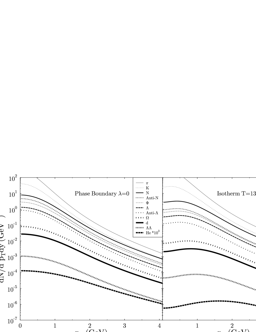
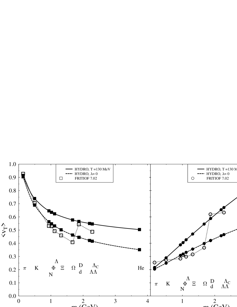
A. Dumitru and D. Rischke solved the relativistic perfect fluid equations assuming longitudinal scaling flow. They used various microscopic models, namely PCM, RQMD, FRITIOF, and HIJING, to assist in estimating the initial conditions. The baryon rapidity density was taken to be 25 and the entropy per baryon was taken to be 200. The formation time of the system was taken as 0.6 fm/c, which is about 1/10 of the radius of a gold nucleus. This resulted in an initial energy density of 17 GeV/fm3 and baryon density of 2.3 times normal nuclear matter density. For a near ideal quark-gluon plasma this yields an initial temperature of 300 MeV and a light quark chemical potential of 47 MeV. The phase transition to hadrons is first order with a critical temperature of 160 MeV (when the baryon chemical potential is zero). The sensitivity of the observed spectra to several different initial density profiles was investigated. They found that the average transverse flow velocity is rather similar to that in central Pb+Pb collisions at the SPS due to the stall of the flow within the mixed phase. Figure 1 shows the calculated transverse momentum spectra for 11 different species of hadrons. The left panel is the distribution immediately after the phase transition is completed, the right panel shows the distribution calculated along the isotherm of MeV. One sees clearly that the flow continues to evolve after the phase transition. It is especially apparent for heavier hadrons. Figure 2 shows average transverse velocity (left panel) and transverse momentum (right panel) as a function of the mass of the hadron. Hydrodynamics predicts a linear increase of the average transverse momentum with mass, whereas FRITIOF alone shows a more complicated dependence on the flavor composition of the hadrons. As can be seen, the results do depend on the hypersurface on which the hadron spectra are computed.
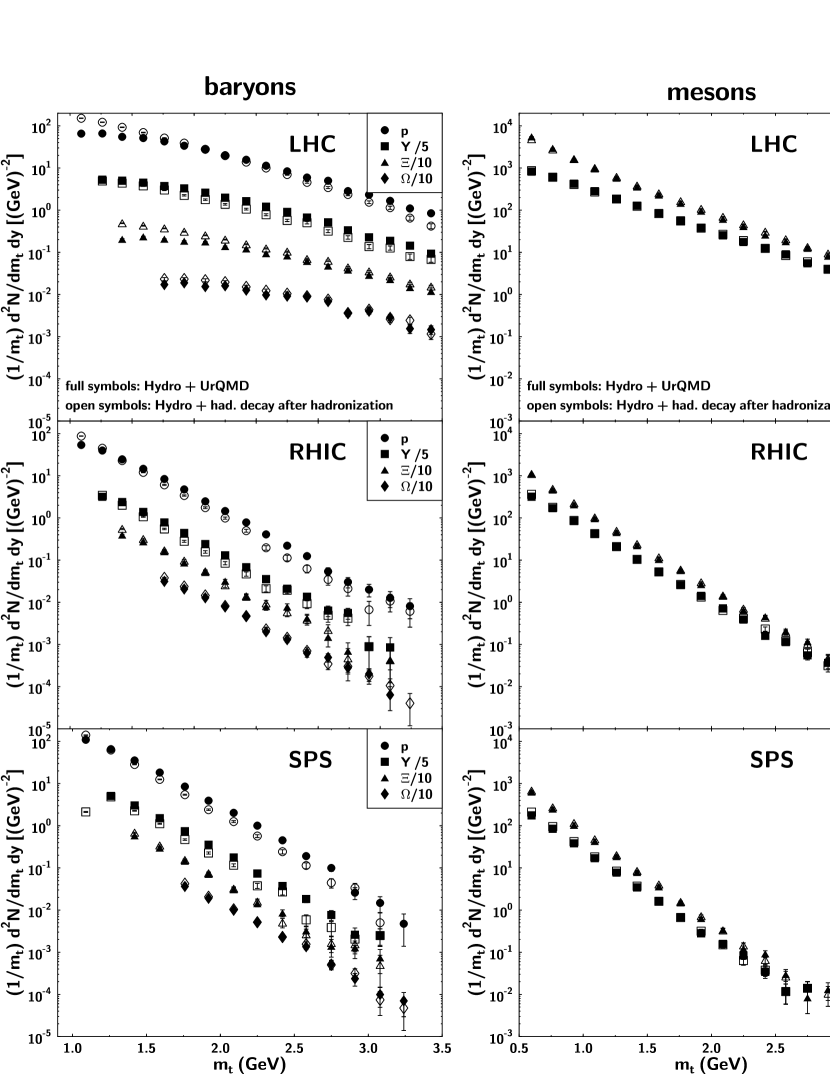
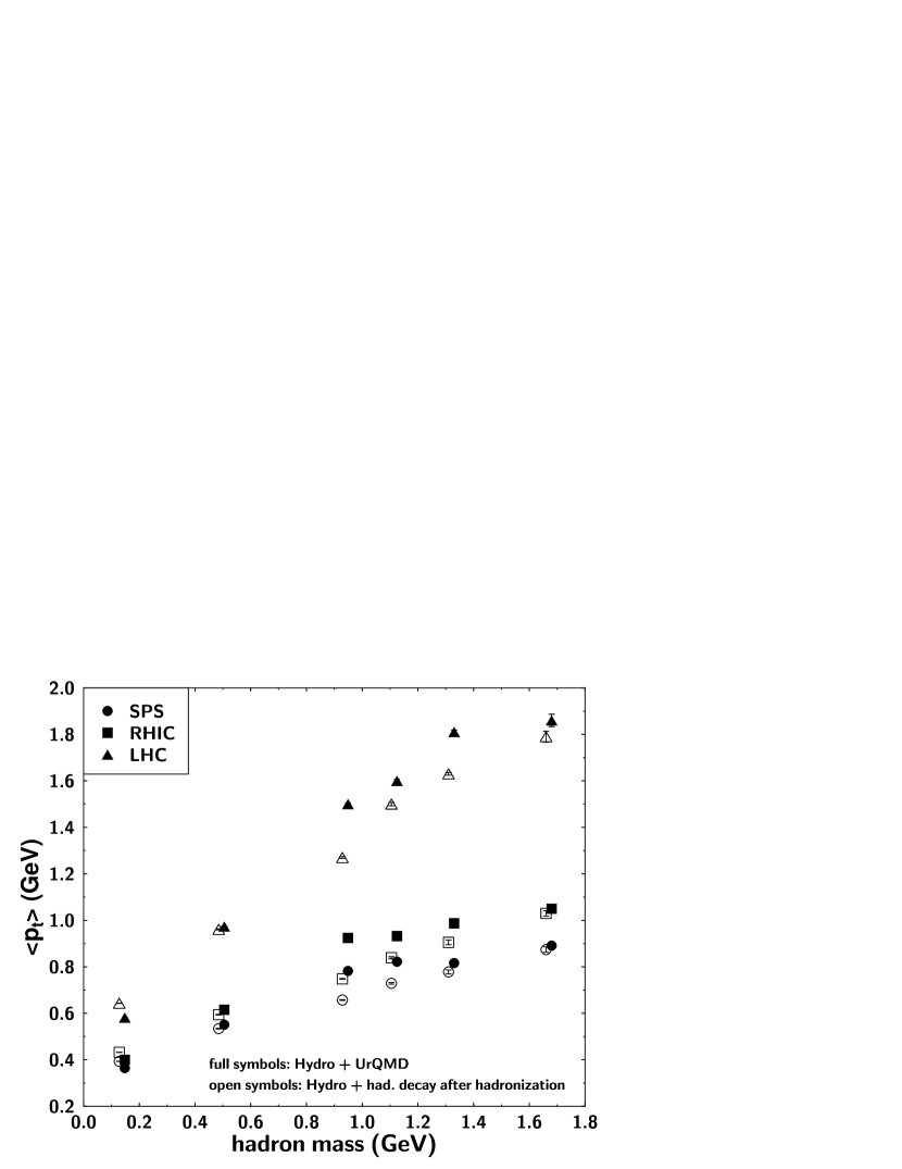
S. Bass and A. Dumitru also solved boost invariant hydrodynamic equations. The initial conditions were essentially identical to those of Dumitru and Rischke. The initial transverse energy and baryon density profile was taken to be proportional to with the transverse radius fm and the formation time 1/10 of that. After the phase transition is complete and the matter has been evolved to a temperature of 130 MeV the hadron spectra are computed using the Cooper-Frye formula, as in Dumitru and Rischke, but the resulting spectra is then used as an initial condition for the hadronic cascade UrQMD. In this way the transition from perfect local thermal equilibrium to free streaming hadrons is done in a more sophisticated manner than making a sudden, abrupt transition from one to the other. The resulting transverse mass distributions for baryons with different strangeness content and for pions and kaons are shown in Figure 3 for SPS, RHIC, and LHC energies. At least for the SPS and RHIC there is not much effect of using UrQMD as the intermediary between hydrodynamic flow and free streaming. Figure 4 shows the average transverse momentum for hadrons as a function of their mass for the three energies. Once again the effect of UrQMD is small but measurable.
These entries nicely illustrate the beautiful evolution of a quark-gluon plasma, through a phase transition, into a hadronic gas and the final nonequilibrium freezeout into free streaming particles. They could be elaborated even more with the use of imperfect fluid dynamics (viscosity and heat conduction) and finite nucleation rates for the phase transition. The main uncertainty is still the choice of initial conditions. The most reasonable choices are to take them from a microscopic model of the early stages of a heavy ion collision, such as these two entries do, or to adjust them so that the computed final state spectra agree with data. Although the second choice is certainly valid and worthwhile it is difficult to refer to it as a prediction.
4 Microscopic Transport Models
The most ambitious entries compute the whole nucleus-nucleus collision from beginning to end on the basis of microscopic dynamics with no assumptions about local equilibrium. By necessity this is done with Monte Carlo techniques. There are two entries in this category which are relevant for strange particle production.
B. Zhang, C.M. Ko, B.-A. Li and Z. Lin take the initial parton distributions from HIJING and evolve them according to their parton cascade model ZPC. They allow the partons to hadronize, after which hadrons interact according to the cascade model ART until all particles free stream to infinity. As with any parton cascade there are uncertainties arising from the nature of infrared singularities in QCD. The predictions for and for all mesons are shown in Figure 5. The main point is that multiple collisions in the partonic and hadronic phases produce more particles than that input from HIJING. The extra particle production occurs in the central rapidity range where the initial particle density is the highest, of course. The kaon abundance is especially enhanced, by about 50%.
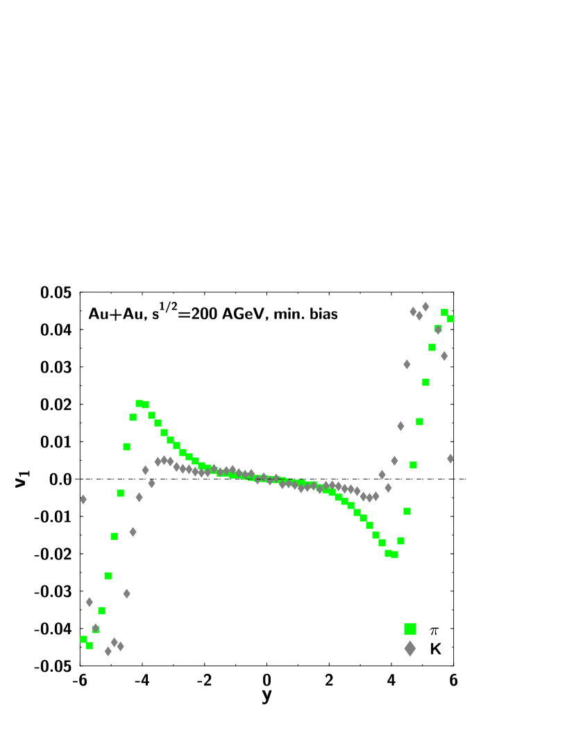
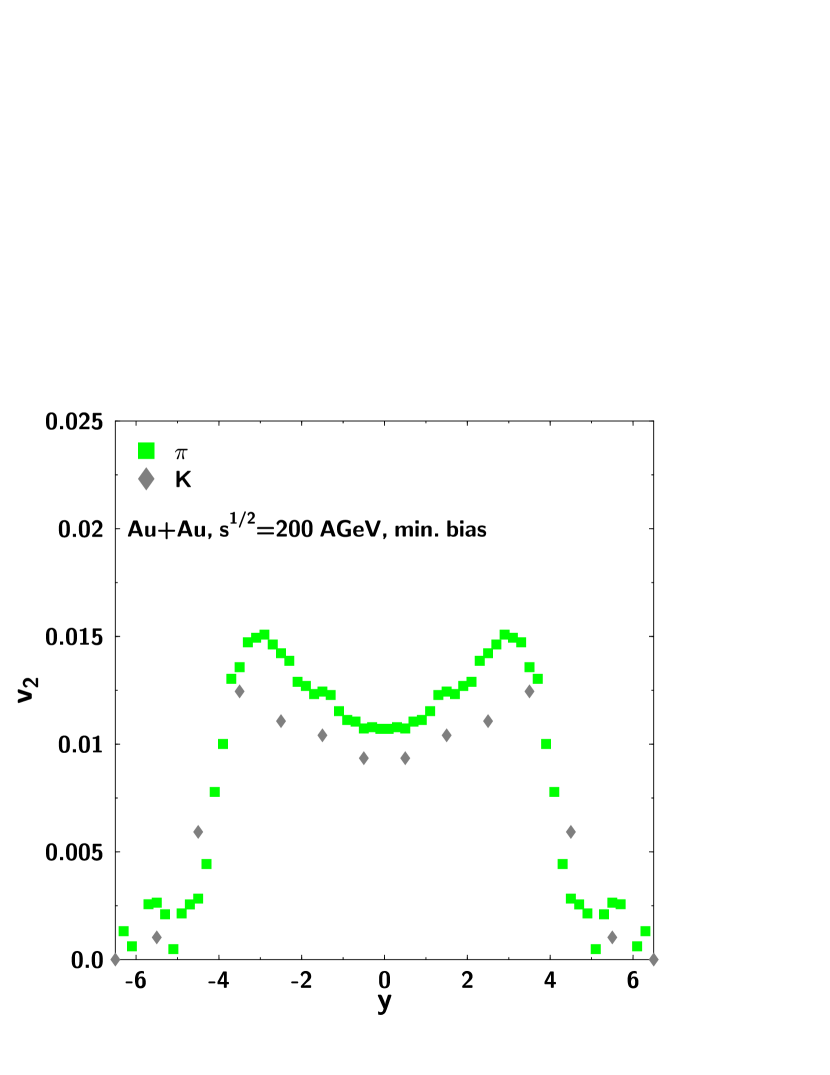
The UrQMD collaboration entry was submitted by M. Bleicher. The UrQMD creates particles at high energies from strings, and at low energies exclusive reactions are parametrized, usually in terms of resonances. It is a very ambitious model which can predict almost anything desired in a heavy ion collision. This also means that it is easier to find fault with it, either in terms of the details of its dynamics, or in terms of predictions not consistent with experimental data. I have selected a subset of all the submitted predictions involving strange hadrons. In Figure 6 are shown the predictions for the rapidity distributions of protons, antiprotons, negative pions, and kaons. In each panel there are two sets of numbers: the open symbols have meson-meson and meson-baryon and certain quark interactions turned off, the full symbols have them all turned on. Just like the previous cascade approach, multiple scattering among the produced particles creates more particles. It also shows that baryons are moved in toward central rapidity from the fragmentation regions. Figure 7 shows the average transverse momentum for pions, kaons, and protons as functions of rapidity. Multiple scatterings increase the mean transverse momentum for protons and kaons, but slightly reduce it for pions. This may be a consequence of the ability of higher energy pions to produce kaons whereas the lower energy pions remain. UrQMD is even so bold as to predict the directed and elliptic flow parameters, and , for every species of hadron. These are shown for pions and kaons in Figures 8 and 9. Pions and kaons flow in about the same way, but the magnitude of the flow coefficients is greater for pions. Similar figures comparing protons, antiprotons, and lambdas may be found at the web site. These observables give information on the degree of equilibration and on the amount of energy loss of the hadrons as they traverse hadronic matter.
Any cascade-like dynamical model requires detailed assumptions about production cross sections, off-shell behavior of propagating particles, formation times, etc. It is very good to see these firm predictions for they can be tested in the very near future!
5 Summary
There is a proverb which says “May you live in interesting times.” The three of us eagerly look forward to comparing all the predictions with RHIC data as they emerge. We should be ready to announce the winner in the summer of 2001. The most exciting outcome would be something that was not predicted!
Acknowledgements
This work was supported by the US Department of Energy under grant DE-FG02-87ER40328.
| 1.25 | 1.5 | 1.5 | 1.5 | 1.60 | |
| 1.03 | 1.025 | 1.03 | 1.035 | 1.03 | |
| [GeV] | 117 | 133 | 111 | 95 | 110 |
| 18 | 16 | 13 | 12 | 12 | |
| 630 | 698 | 583 | 501 | 571 | |
| 1.19 | 1.15 | 1.19 | 1.22 | 1.19 | |
| 1.74 | 1.47 | 1.47 | 1.45 | 1.35 | |
| 1.85 | 1.54 | 1.55 | 1.55 | 1.44 | |
| 0.89 | 0.91 | 0.89 | 0.87 | 0.89 | |
| 0.19 | 0.16 | 0.16 | 0.16 | 0.15 | |
| 0.20 | 0.17 | 0.17 | 0.17 | 0.16 | |
| 0.94 | 0.95 | 0.94 | 0.93 | 0.94 | |
| 0.147 | 0.123 | 0.122 | 0.122 | 0.115 | |
| 0.156 | 0.130 | 0.130 | 0.131 | 0.122 | |
| 1 | 1 | 1 | 1 | 1 | |
| 0.15 | 0.13 | 0.13 | 0.13 | 0.12 | |
| 0.19 | 0.16 | 0.16 | 0.16 | 0.15 | |
| 1.05 | 1.04 | 1.05 | 1.06 | 1.05 |
| 1.25 | 1.03 | 17 | 25∗ | 21 | 44 | 39 | 31 | 27 | 17 | 16 | 1.2 |
|---|---|---|---|---|---|---|---|---|---|---|---|
| 1.5 | 1.025 | 13 | 25∗ | 22 | 36 | 33 | 26 | 23 | 13 | 11 | 0.7 |
| 1.5 | 1.03 | 16 | 25∗ | 21 | 37 | 33 | 26 | 23 | 12 | 11 | 0.7 |
| 1.5 | 1.035 | 18 | 25∗ | 21 | 36 | 32 | 26 | 22 | 11 | 10 | 0.7 |
| 1.60 | 1.03 | 15 | 25∗ | 21 | 34 | 30 | 24 | 21 | 10 | 9.6 | 0.6 |