Abstract

The relations between the strengths of spin-isospin transition operators extracted from direct nuclear reactions, magnetic scattering of electrons and processes of semi-lepton weak interaction are discussed.

1. Introduction

The studies of the spin-isospin excitations in atomic nuclei have a long history. Detailed discussions of it are given by the authors of recent reviews [1, 2]. We touch here only a few points important for our purposes. The first manifestation of spin-isospin transitions was detected in beta-decay as Gamow-Teller transitions ($\Delta J^{\pi}=1^{+}$) for which

$$\log ft_{1/2}={6135\over(g_{A}/g_{V})^{2}B^{\pm}(GT)}.$$

Here the strength of the Gamow-Teller transition is introduced as

$$B^{\pm}_{f}(GT)={1\over 2J_{f}+1}\biggl{|}\langle J_{f}\biggl{\|}\sum_{k=1}^{A}\sigma_{k}\,t^{\pm}_{k}\biggr{\|}J_{i}\rangle\biggr{|}^{2}\,.$$ (1)

In this paper we will only discuss the transitions $0^{+}\rightarrow 1^{+}$. The discovery of isobar analog states in $(p,n)$ reactions was followed by the prediction of the a new nuclear collective excitation – the giant GT resonance – as the reason of lack of $\sigma t^{-}$ strength observed in $\beta$-decay studies. At the beginning of 1980-s giant GT resonances were experimentally discovered and studied in $(p,n)$ and other nuclear charge-exchange reactions (CEX) at intermediate energies. Using some additional assumptions, it was shown in [3] that the $0^{\circ}\,(p,n)$ cross sections are proportional to $B(GT)$. The comparison of the $B(GT)$ values extracted from the cross sections of CEX reactions with those obtained from $\beta$-decay reveals that some differences exist between them [4]. The origin of these differences has been explained by the fact that transitions with small $B(GT)$ are observed even in fast beta decay. For small $B(GT)$, however, other spin-multipoles contribute strongly to the CEX cross sections leading to a considerable deviation from the proportionality between the $0^{\circ}$ cross sections and the $B(GT)$ values. Therefore large errors may appear in $B(GT)$’s obtained from the CEX cross sections [5].

Recent experiments on exclusive muon capture in $sd$-shell nuclei [6] give the possibility to compare the characteristics of strong GT transitions measured in weak interaction processes to those obtained from the CEX reactions. The energy released in nuclear muon capture is determined by the muon mass. Limitations on the transition energy, that exist in beta decay, are absent in muon capture. During muon capture the nucleus acquires a non-zero linear momentum. Therefore the kinematics in muon capture differs from that in beta decay and zero-angle CEX reactions. For this reason the matrix elements for $0^{+}\rightarrow 1^{+}$ transitions obtained in muon capture can not be compared directly to the $B(GT)$’s extracted from $(p,n)$ reactions. One is therefore forced to ask a different question, namely, as to what extend the wave functions of the isovector states will simultaneously describe the experimental $B(GT)$’s and the rates of ordinary muon capture ($\Lambda_{f}$).

2. The nuclear muon capture rate

We base our calculations of exclusive muon capture rates on the approach described in [7]. In case that the matrix elements of the operator $\displaystyle\sum_{k=1}^{A}j_{0}(E_{\nu}r_{k})\,\sigma_{k}\,t^{+}_{k}$ dominates, the rates for the partial transitions $0^{+}_{\rm g.s.}\rightarrow 1^{+}_{f}$ are give by (only the final result is shown here)

$$\matrix{\Lambda_{f}\approx&\displaystyle{2\over 3}\,V\,g^{2}_{A}\,[101]^{2}\,\biggl{\{}1+{2\over 3}\eta+{8\over 3}{{g_{V}+g_{M}}\over g_{A}}\eta-{2\over 3}{g_{P}\over g_{A}}\eta+{1\over 3}\bigl{(}{g_{P}\over g_{A}}\eta\bigr{)}^{2}\hfill\cr\vskip 6.0pt plus 2.0pt minus 2.0pt\cr&\displaystyle+\,\sqrt{8\over 9}\biggl{[}2\bigl{(}1+{{g_{V}+g_{M}}\over g_{A}}-{g_{P}\over g_{A}}\bigr{)}\eta+\bigl{(}{g_{P}\over g_{A}}\eta\bigr{)}^{2}\biggr{]}\,{{[121]}\over{[101]}}\hfill\cr\vskip 6.0pt plus 2.0pt minus 2.0pt\cr&\displaystyle+\,2\,\bigl{(}1-{g_{P}\over g_{A}}\bigr{)}\,\eta\,{[111p]\over M\,[101]}-\sqrt{8\over 9}\,{g_{V}\over g_{A}}\,{[011p]\over M\,[101]}\biggr{\}}\,,\hfill\cr}$$ (2)

where $\displaystyle\eta={E_{\nu}\over 2\,M_{p}}$ and the nuclear matrix elements are defined by

$$\matrix{[101]&=\displaystyle\sqrt{1\over 4\pi}\langle 1^{+}_{f}\parallel\sum_{k=1}^{A}\varphi_{\mu}(r_{k})\,j_{0}(E_{\nu}r_{k})\,Y_{0}(\hat{r}_{k})\,\sigma_{k}\,t^{+}_{k}\parallel 0^{+}_{\rm g.s.}\rangle\,,\hfill\cr[121]&=\displaystyle\sqrt{1\over 4\pi}\langle 1^{+}_{f}\parallel\sum_{k=1}^{A}\varphi_{\mu}(r_{k})\,j_{2}(E_{\nu}r_{k})\,\bigr{[}Y_{2}(\hat{r}_{k})\otimes\sigma_{k}\bigr{]}_{1}\,t^{+}_{k}\parallel 0^{+}_{\rm g.s.}\rangle\,,\hfill\cr[111p]&=\displaystyle\sqrt{1\over 4\pi}\langle 1^{+}_{f}\parallel\sum_{k=1}^{A}\varphi_{\mu}(r_{k})\,j_{1}(E_{\nu}r_{k})\,\bigr{[}Y_{1}(\hat{r}_{k})\otimes\nabla_{k}\bigr{]}_{1}\,t^{+}_{k}\parallel 0^{+}_{\rm g.s.}\rangle\,,\hfill\cr[011p]&=\displaystyle\sqrt{1\over 12\pi}\langle 1^{+}_{f}\parallel\sum_{k=1}^{A}\varphi_{\mu}(r_{k})\,j_{1}(E_{\nu}r_{k})\,Y_{1}(\hat{r}_{k})\,\bigr{(}\vec{\nabla}_{k},\vec{\sigma}_{k}\bigr{)}\,t^{+}_{k}\parallel 0^{+}_{\rm g.s.}\rangle\,.\cr}$$

Here $\varphi_{\mu}(r)$ is muon radial wave function. We approximate $\varphi_{\mu}$, as is done usually for light and medium nuclei, by the average value calculated in [8].

3. Comparison between calculations and
experimental data

The calculations have been carried out on the basis of a many-particle shell model using the Hamiltonian of B.H. Wildenthal [9] and an unrestricted $sd$-shell space. The computer code OXBASH [10] has been used in the calculations. Theoretical and experimental GT- and $M1$-strength functions are presented in Fig. 1. The theoretical results obtained with the eigenfunctions of Wildenthal’s Hamiltonian are marked by (a). The $B(GT)$ for the $1^{+}$ states with excitation energies below $6$ MeV are shown in the upper left part of Fig. 1. The energies are measured from the ground state of ${}^{28}{\rm P}$. The experimental GT strength function was obtained from the cross sections for the ${}^{28}{\rm Si}(p,n){}^{28}{\rm P}$ reaction [12]. All states with excitation energy below $5$ MeV are shown in Fig. 1. Only a small fraction of the whole experimental GT strength goes to the states with higher excitation energies [12]. Additionally, the exact spins and parities of high-lying states have not been determined experimentally. Because of these two reasons we neglect in the following considerations the high-lying states which are not shown in Fig. 1. In the energy region up to $12.6$ MeV one observes an experimental $B(GT)$ strength of $2.595$; the $B(GT)$’s summed over the states shown in Fig. 1 amounts to $2.301$. The theoretical $B(GT)$’s summed over the first 10 eigestates with $J^{\pi},T=1^{+},1$ (shown in Fig. 1) give $3.492$. Therefore a rather standard value of GT quenching $\displaystyle{\Sigma B_{\rm exper.}(GT)\over\Sigma B_{\rm theor.}(GT)}=0.66$ is obtained from this comparison.

Figure 1 shows also the theoretical and experimental $M1$ strength functions. It is known [11] that the shell model with the Hamiltonian [9] reproduces well the energies of isovector $1^{+}$ states in ${}^{28}{\rm Si}$. But the theoretical dependence of the $B(M1)$ values on excitation energy differs considerably from the experimental one, obtained in [13]. The calculations were carried out with the “free” value of $g_{s}$ and the summed theoretical $B(M1)$ is larger than the experimental one : $\displaystyle{\Sigma\,B_{\rm exper.}(M1)\over\Sigma\,B_{\rm theor.}(M1)}={7.360\over 8.623}=0.85$. However, as can be seen in Fig. 1, even in that case the experimental $B(M1)$ exceeds considerably the theoretical value for the strongest transition which goes to the isovector $1^{+}$ state with energy $11.445$ MeV.

Therefore we can conclude that the shell model with the Hamiltonian [9] describes qualitatively the main features of GT and $M1$ strength functions in the sense that small theoretical $B(GT)$’s and $B(M1)$’s correspond to small experimental values. However, the theoretical distributions of the transition strength over the states which absorb the largest part of the total strength differ considerably from the experimental strength functions.

According to (2), the nuclear matrix element $[101]$, having the $\sigma t^{+}$ operator as the spin-angular part, contributes mainly to the rate in fast allowed muon capture. Therefore, the differences between theoretical and experimental values of $B(GT)$ and $B(M1)$ led to the discrepancies between theoretical and experimental values of $\Lambda_{f}$’. The $\Lambda_{f}$’s calculated with the eigenfunctions of the Wildenthal Hamiltonian are shown in Table 1 in column (a). Also, the values of $B(M1)$ and $B(GT)$ for the members of the same isotopic triplets are presented in the Table together with the corresponding experimental numbers. The only conclusion, which one can make comparing experimental data to results of calculation (a), is that the difficulties in description of GT and $M1$ transitions have there counterpart in the description of muon capture rates.

In this situation it might be reasonable to use the available experimental information concerning GT and $M1$ strength functions in the calculations of muon capture rates. For that purpose the orthogonal transformation, acting in the subspace spanned by the wave functions of the isovector $1^{+}$ states, was suggested in [14]. According to this paper the parameters of the transformation should be chosen such that the strength functions of GT and $M1$ transitions calculated with transformed wave functions coincide in shape (up to a constant factor) with the experimental GT and $M1$ strength functions. Therefore, the transformation parameters do not dependent on any relation between the experimental and theoretical values of the summed strengths of GT and $M1$ transitions and are determined by the shapes of experimental GT and $M1$ strength functions only. The orthogonality of the transformation will support the mutual orthogonality and normalization of the obtained wave functions. For the same reason, the theoretical total GT and $M1$ transition strength will be conserved.

The isotopic invariance of strong interactions assures that the transformation of the isovector $1^{+}$ states carried out in ${}^{28}{\rm P}$ will induce the transformations of the $1^{+},1$ states in ${}^{28}{\rm Si}$ and ${}^{28}{\rm Al}$. In addition, the transformation matrix will not depend on the value of the third component of the total isospin. Therefore exactly the same transformation will apply for the corresponding subspaces of the wave functions for ${}^{28}{\rm Si}$ and ${}^{28}{\rm Al}$.

The next section describes how this transformation can be constructed.

4. Transformation of wave functions

The transformation of wave functions of excited states

$$\phi_{k}\rightarrow\psi_{k}=U_{k,k^{\prime}}\,\phi_{k^{\prime}}\qquad(k=1,2,\ldots,N)$$

causes a transformation of the transition matrix elements

$$\langle\phi_{k}|{\cal O}|\Phi\rangle\rightarrow\langle\psi_{k}|{\cal O}|\Phi\rangle=U^{\ast}_{k,k^{\prime}}\,\langle\phi_{k^{\prime}}|{\cal O}|\Phi\rangle=\langle\phi_{k^{\prime}}|{\cal O}|\Phi\rangle\,U^{{\dagger}}_{k^{\prime},k}.$$

Considering the transformation within the subspace of the multiparticle wavefunction as a transformation in a vector space with the transition amplitudes as basis vectors will simplify considerably the determination of the transformation matrix.

An orthogonal $N\times N$ matrix is determined through $N(N-1)/2\,$ free parameters. To reduce the number of required parameters one should use matrices of less general structure. The simplest orthogonal transformation of a vector is its reflection on a plane [15, 16]

$$v=v_{\parallel}+v_{\perp}\rightarrow v^{\prime}=v_{\parallel}-v_{\perp}\ ,$$

Here the vector $v_{\parallel}$ is parallel to the plane and $v_{\perp}$ is perpendicular to the plane. If the plane is determined by the equation $(b,x)=b_{k}x_{k}=0,$ where $b$ is a non-zero vector, $(b,b)>0,$ then according to [15, 16] the transformation is given by

$$v_{k}\rightarrow v^{\prime}=R(b)\,v\quad{\rm with}\quad R_{k,l}(b)=\delta_{k,l}-2\,{b_{k}b_{l}\over(b,b)}\ .$$ (3)

If $|u|=|w|$ one can convert $u$ into $w$ and vice versa by the transformation (3) with $b=u-w$.

From the calculations within the shell model we know the vector, built up from the theoretical GT amplitudes. A second vector is assembled from the experimental amplitudes. After proper normalization the matrix (3) can be constructed. However from the experiment we can get only the absolute values of the transition amplitudes. Therefore we are forced to consider all possible distributions of signs within the “experimental vector”. Each distribution has its own reflection matrix, which will transform the wave functions in such a way that the new theoretical GT strength function will coincide in shape with the experimental one. In order to select the best transformation we consider the $M1$ strength function in ${}^{28}{\rm Si}$. Due to isotopic invariance the $1^{+}$ states in ${}^{28}{\rm Si}$ and ${}^{28}{\rm P}$ are transformed by the same matrix. Therefore, the theoretical $M1$ strength function will be changed too. The magnetic dipole transition operator differs from the GT transition operator and the vectors built up of GT and $M1$ amplitudes will be linearly independent. Therefore, the transformed theoretical $M1$ strength function will have a different shape from the experimental one. We use that transformation which leads to the smallest deviation between the theoretical and experimental $M1$ shapes.

5. Calculations with transformed wave functions

The GT and $M1$ strength functions calculated with the transformed wave functions are presented on the right hand side of Fig. 1, marked by (b). The subspace, in which the transformation acts, includes all the states shown in Fig. 1. The transformation causes a significant redistribution of transition strengths over the excitation energies. As a result, the shape of GT strength function is exactly restored and the shape of the $M1$ strength function is approximately reproduced. The muon capture rates calculated with the transformed wave functions are given in column (b) of Table 1. The new theoretical rates are very closed to the experimental ones. The errors in $\Lambda_{f}$ are estimations of the uncertainties in the calculated rates induced by errors in the experimental values of $B(GT)$’s and $B(M1)$’s, which were used in the construction of the transformation. It should be pointed out again that the experimental values of $B(GT)$ and $B(M1)$ themselves have not been used in transformation matrix, only the shapes of the experimental GT and $M1$ strength functions were important for the transformation. Also, no effective charges were introduced in the calculations. It is reasonable to compare $B(GT)$ and $B(M1)$ calculated with the transformed wave functions to the experimental values. The result is given in column (b) of Table 1.

The calculations with the transformed wave functions, carried out for the strongest transitions, produce surprising results: the theoretical OMC rates are very close to the experimental values; the theoretical $B(M1)$’s are close to the experimental ones; but the theoretical $B(GT)$’s are $1.5$ times larger than those extracted from the cross sections of reaction ${}^{28}{\rm Si}(p,n){}^{28}{\rm P}$. Because of the similarity of the spin-isospin parts of the operators describing CEX reactions, magnetic scattering of electrons and muon capture, this disagreement is unexpected.

6. Conclusions

We have constructed a set of wave functions of the excited isovector $1^{+}$ states in $A=28$ nuclei starting from the wave functions calculated within a many-particle shell model using the Hamiltonian [9] and introducing phenomenological corrections by means of an orthogonal transformation in a subspace of shell model wave functions. Then, several characteristics of the spin-isospin transitions were calculated with the new wave functions. The calculations were carried out without introducing any effective charges. The theoretical results being compared to experimental data show that for the strongest isovector $0^{+}\rightarrow 1^{+}$ transitions: i) the theoretical OMC rates are very close to the experimental values; ii) the theoretical $B(M1)$’s are close to the experimental ones; iii) the theoretical $B(GT)$’s are $1.5$ times larger than those extracted from the cross sections of the reaction ${}^{28}{\rm Si}(p,n){}^{28}{\rm P}$. This disagreement is unexpected mainly due the to similarity of spin-isospin parts of the operators describing CEX reactions, magnetic scattering of electrons and muon capture.

We have shown that experimental data on partial muon capture rates can be used to obtaine important spectroscopic information, because fast spin-flip transitions were observed and the rates of weak interaction processes have been measured for such fast transitions.

In contrast to the general accepted opinion the relation between cross sections of CEX reactions and $B(GT)$ could be quite complicated even for the strong GT transitions. It seems to be necessary to investigate how spin-quadrupole transitions and two-step processes could contribute to cross sections of CEX reactions even for strong GT transitions.

Table 1: Properties of spin-isospin transitions in $A=28$ nuclei. References to experimental data and details of the calculations are given in the text.

$$E_{f}$$ experiment calculations

MeV  (a) (b)

(in )  for

(in ) for

for

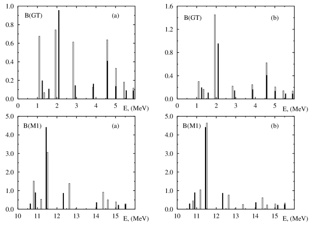
Figure 1: Strength functions of GT and $M1$ transitions in ${}^{28}{\rm Si}$. The experimental data are shown by closed bars; the results of calculations – as open bars. The calculations (a) have been carried out with eigenfunctions of the Hamiltonian [9], (b) – with the transformed wave functions.

References

- [1] F. Osterfeld, Rev. Mod. Phys. 64, 491 (1992).
- [2] W.P. Alford, B.M. Spicer, Adv. Nucl. Phys. 24, 2 (1998).
- [3] C.D. Goodman, et al., Phys. Rev. Lett. 44, 1755 (1980).
- [4] T.N. Taddeucci, et al., Nucl. Phys. A 469, 125 (1987); E.G. Adelberger, et al., Phys. Rev. Lett. 67, 3658 (1991).
- [5] S.M. Austin, N. Anantaraman, W.G. Love, Phys. Rev. Lett. 73, 30 (1994).
- [6] T.P. Gorringe, et al., Phys. Rev. C 60, 055501 (1999).
- [7] V.V. Balashov, R.A. Eramzhyan, Rev. At. En. (Vienne) 5, 3 (1967).
- [8] K.W. Ford, J.G. Wills, Nucl. Phys. 35, 295 (1962).
- [9] B.H. Wildenthal, Prog. Part. Nucl. Phys. 11, 5, (1984).
- [10] B.A. Brown, A. Etchegoyen, W.D.M. Rae, OXBASH, Report No. 524 (MSU cyclotron Laboratory, Michigan, U.S.A., 1986).
- [11] P.M. Endt, J.G.L. Booten, Nucl. Phys. A 555, 499, (1993).
- [12] B.D. Anderson, et al., Phys. Rev. C 43, 50 (1991); P. von Neumann-Cosel, et al., Phys. Rev. C 55, 532 (1997).
- [13] C. Lüttge, et al., Phys. Rev. C 53, 127 (1996); Y. Fujita, et al., Phys. Rev. C 55, 1137 (1997).
- [14] V.A. Kuz’min, T.V. Tetereva, Preprint No. E4-99-210, JINR (Joint Institute for Nuclear Research, Dubna, Russia, 1999) will be published in Phys. At. Nucl.
- [15] E. Cartan, Leçons sur la theórie des spineurs (Actualités Scientifiques et Industrielles 643, 701: Paris, 1938).
- [16] A.S. Householder, The theory of matrices in Numerical Analysis (New York: Blaisdel, 1964).