Effective Field Theory with Two and Three Nucleons

Abstract

Progress in the Effective Field Theory of two and three nucleon systems is sketched, concentrating on the low energy version in which pions are integrated out as explicit degrees of freedom. Examples given are calculations of deuteron Compton scattering, three body forces and the triton, and $\mathrm{nd}$ partial waves.

1 Foundations of Effective Nuclear Theory

This presentation is a cartoon of the Effective Field Theory (EFT) of two and three nucleon systems as it emerged in the last three years, using a lot of words and figures, and a few cheats. For details, I refer to the bibliographies in [1] as well as a recent review [2], and papers with J.-W. Chen, R.P. Springer and M.J. Savage [3], P.F. Bedaque [4, 5], and F. Gabbiani [5]. I will mainly concentrate on the theory in which pions are integrated out as explicit degrees of freedom, but also comment on the extensions to include pions. B. Holstein’s talk [6] provides an introduction to EFT, and E. Epelbaum’s contribution [7] investigates one of the two proposals to include pions in more detail.

Effective Field Theory methods are largely used in many branches of physics where a separation of scales exists [6]. In low energy nuclear systems, the scales are, on one side, the low scales of the typical momentum of the process considered and the pion mass, and on the other side the higher scales associated with chiral symmetry and confinement. This separation of scales produces a low energy expansion, resulting in a description of strongly interacting particles which is systematic and rigorous. It is also model independent (meaning, independent of assumptions about the non-perturbative QCD dynamics): Given that QCD is the theory of strong interactions and that chiral symmetry is broken via the Goldstone mechanism, Wilson’s renormalisation group arguments show that there is only one local low energy field theory which originates from it: Chiral Perturbation Theory and its extension to the many-nucleon system discussed here.

1.1 The Lagrangean

Three main ingredients enter the construction of an EFT: The Lagrangean, the power counting and a regularisation scheme. First, the relevant degrees of freedom have to be identified. In his original suggestion how to extend EFT methods to systems containing two or more nucleons, Weinberg [8] noticed that below the $\Delta$ production scale, only nucleons and pions need to be retained as the infrared relevant degrees of freedom of low energy QCD. Because at these scales the momenta of the nucleons are small compared to their rest mass, the theory becomes non-relativistic at leading order in the velocity expansion, with relativistic corrections systematically included at higher orders. The most general chirally invariant Lagrangean consists hence of contact interactions between non-relativistic nucleons, and between nucleons and pions, with the first terms of the form

$${\mathcal{L}}_{\mathrm{NN}} = N^{\dagger}(\mathrm{i}\partial_{0}+\frac{\vec{\partial}^{2}}{2M})N+\;\frac{f_{\pi}^{2}}{8}\;\mathrm{tr}[(\partial_{\mu}\Sigma^{\dagger})(\partial^{\mu}\Sigma)]\;+\;g_{A}N^{\dagger}\vec{A}\cdot\sigma N\;-$$

$$-\;C_{0}(N^{\mathrm{T}}P^{i}N)^{\dagger}\ (N^{\mathrm{T}}P^{i}N)\;+\;\frac{C_{2}}{8}\left[(N^{\mathrm{T}}P^{i}N)^{\dagger}(N^{\mathrm{T}}P^{i}(\stackrel{{\scriptstyle\scriptscriptstyle\rightarrow}}{{\partial}}-\stackrel{{\scriptstyle\scriptscriptstyle\leftarrow}}{{\partial}})^{2}N)+\mathrm{H.c.}\right]+\dots,$$

where $N={p\choose n}$ is the nucleon doublet of two-component spinors and $P^{i}$ is the projector onto the iso-scalar-vector channel, $P^{i,\,b\beta}_{a\alpha}=\frac{1}{\sqrt{8}}(\sigma_{2}\sigma^{i})_{\alpha}^{\beta}(\tau_{2})_{a}^{b}$. The iso-vector-scalar part of the $\mathrm{NN}$ Lagrangean introduces more constants $C_{i}$ and interactions and has not been displayed for convenience. The field $\xi(x)=\sqrt{\Sigma}=e^{\mathrm{i}\Pi/f_{\pi}}$ describes the pion. $D_{\mu}=\partial_{\mu}+V_{\mu}$ is the chirally covariant derivative, and $A_{\mu}=\frac{\mathrm{i}}{2}(\xi\partial_{\mu}\xi^{\dagger}-\xi^{\dagger}\partial_{\mu}\xi)$ ($V_{\mu}$) the axial (vector) pionic current. The interactions involving pions are severely restricted by chiral invariance. As such, the theory is an extension of Chiral Perturbation Theory and Heavy Baryon Chiral Perturbation Theory to the many nucleon system. Like in its cousins, the coefficients of the low energy Lagrangean encode all short distance physics – branes and strings, quarks and gluons, resonances like the $\Delta$ or $\rho$ – as strengths of the point-like interactions between particles. As it is not possible yet to derive these constants by solving QCD e.g. on the lattice, the most practical way to determine them is by fitting to experiment.

1.2 The Power Counting

Because the Lagrangean (1.1) consists of infinitely many terms only restricted by symmetry, an EFT may at first sight suffer from lack of predictive power. Indeed, as the second part of an EFT formulation, predictive power is ensured by establishing a power counting scheme, i.e. a way to determine at which order in a momentum expansion different contributions will appear, and keeping only and all the terms up to a given order. The dimensionless, small parameter on which the expansion is based is the typical momentum $Q$ of the process in units of the scale $\Lambda_{\mathrm{NN}}$ at which the theory is expected to break down. Values for $\Lambda_{\mathrm{NN}}$ and $Q$ have to be determined from comparison to experiments and are a priori unknown. Assuming that all contributions are of natural size, i.e. ordered by powers of $Q$, the systematic power counting ensures that the sum of all terms left out when calculating to a certain order in $Q$ is smaller than the last order retained, allowing for an error estimate of the final result.

For extremely small momenta, the pion does not enter as explicit degree of freedom, and all its effects are absorbed into the coefficients $C_{i}$. This Effective Nuclear Theory with pions integrated out (ENT(${\pi\hskip-5.50003pt/}$)) was recently pushed to very high orders in the two-nucleon sector [9] where accuracies of the order of $1\%$ were obtained. It can be viewed as a systematisation of Effective Range Theory with the inclusion of relativistic and short distance effects traditionally left out in that approach. Because of non-analytic contributions from the pion cut, the breakdown scale of this theory must be of the order ${}^{\pi\hskip-2.79996pt/}\Lambda_{\mathrm{NN}}\sim m_{\pi}$. For the ENT with explicit pions, we would suspect the breakdown scale to be of the order of $M_{\Delta}-M$, since the $\Delta$ is not an explicit degree of freedom in (1.1).

Even if calculations of nuclear properties were possible starting from the underlying QCD Lagrangean, EFT simplifies the problem considerably by factorising it into a long distance part which contains the infrared-relevant physics and is dealt with by EFT methods and a short distance part, subsumed into the coefficients of the Lagrangean. QCD therefore “only” has to provide these constants, avoiding full-scale calculations of e.g. bound state properties of two nuclear systems using quarks and gluons. EFT provides an answer of finite accuracy because higher order corrections are systematically calculable and suppressed in powers of $Q$. Hence, the power counting allows for an error estimate of the final result, with the natural size of all neglected terms known to be of higher order. Relativistic effects, chiral dynamics and external currents are included systematically, and extensions to include e.g. parity violating effects are straightforward. Gauged interactions and exchange currents are unambiguous. Results obtained with EFT are easily dissected for the relative importance of the various terms. Because only $S$-matrix elements between on-shell states are observables, ambiguities nesting in “off-shell effects” are absent. On the other hand, because only symmetry considerations enter the construction of the Lagrangean, EFTs are less restrictive as no assumption about the underlying QCD dynamics is incorporated. Hence the proverbial quib that “EFT parameterises our ignorance”.

In systems involving two or more nucleons, establishing a power counting is complicated because unnaturally large scales have to be accommodated: Given that the typical low energy scale in the problem should be the mass of the pion as the lightest particle emerging from QCD, fine tuning is required to produce the large scattering lengths in the $\mathrm{S}$ wave channels ($1/a^{{}^{1}\mathrm{S}_{0}}=-8.3\;\mathrm{MeV},\;1/a^{{}^{3}\mathrm{S}_{1}}=36\;\mathrm{MeV}$). Since there is a bound state in the ${}^{3}\mathrm{S}_{1}$ channel with a binding energy $B=2.225\;\mathrm{MeV}$ and hence a typical binding momentum $\gamma=\sqrt{MB}\simeq 46\;\mathrm{MeV}$ well below the scale $\Lambda_{\mathrm{NN}}$ at which the theory should break down, it is also clear that at least some processes have to be treated non-perturbatively in order to accommodate the deuteron, i.e. an infinite number of diagrams has to be summed.

For simplicity, let us first turn to the EFT in which the pion is integrated out into the coefficients ${}^{\pi\hskip-2.79996pt/}C_{i}$ of the Lagrangean. Here, a way to incorporate this fine tuning into the power counting was suggested by Kaplan, Savage and Wise [12], and by van Kolck [13]. At very low momenta, contact interactions with several derivatives – like $p^{2}\,{}^{\pi\hskip-2.79996pt/}C_{2}$ – should become unimportant, and we are left only with the contact interactions proportional to ${}^{\pi\hskip-2.79996pt/}C_{0}$. The leading order contribution to nucleons scattering in an $\mathrm{S}$ wave comes hence from four nucleon contact interactions and is summed geometrically as in Fig. 1 in order to produce the shallow real bound state, i.e. the deuteron.

$\mbox{\parbox{32.50008pt}{ \fmfgraph*(25,25) \fmfleft{i} \fmfright{o} \fmf{double,width=thin}{i,o} }}\hskip 5.0pt=\hskip 5.0pt\mbox{\parbox{39.00009pt}{ \fmfgraph*(30,25) \fmfleft{i1,i2} \fmfright{o1,o2} \fmf{vanilla,width=thin}{i1,v,o2} \fmf{vanilla,width=thin}{i2,v,o1} }}+\mbox{\parbox{58.50014pt}{ \fmfgraph*(45,25) \fmfleft{i1,i2} \fmfright{o1,o2} \fmf{vanilla,width=thin,tension=6}{i1,v1} \fmf{vanilla,width=thin,tension=6}{v2,o2} \fmf{vanilla,width=thin,tension=6}{i2,v1} \fmf{vanilla,width=thin,tension=6}{v2,o1} \fmf{vanilla,width=thin,left=0.5}{v1,v2} \fmf{vanilla,width=thin,left=0.5}{v2,v1} }}+\mbox{\parbox{81.90019pt}{ \fmfgraph*(63,25) \fmfleft{i1,i2} \fmfright{o1,o2} \fmf{vanilla,width=thin,tension=6}{i1,v1} \fmf{vanilla,width=thin,tension=6}{v2,o2} \fmf{vanilla,width=thin,tension=6}{i2,v1} \fmf{vanilla,width=thin,tension=6}{v2,o1} \fmf{vanilla,width=thin,left=0.7}{v1,v3} \fmf{vanilla,width=thin,left=0.7}{v3,v1} \fmf{vanilla,width=thin,left=0.7}{v2,v3} \fmf{vanilla,width=thin,left=0.7}{v3,v2} }}+\;\dots\;=\;\displaystyle\frac{-{}^{\pi\hskip-2.79996pt/}C_{0}}{1-\rule{0.0pt}{16.0pt}\mbox{\parbox{31.20007pt}{ \fmfgraph*(25,12) \fmfleft{i} \fmfright{o} \fmf{vanilla,width=thin,left=0.5}{i,o} \fmf{vanilla,width=thin,left=0.5}{o,i} }}}$

Figure 1: Re-summation of the contact interactions into the deuteron propagator.

How to justify this? Dimensional analysis allows any diagram to be estimated by scaling momenta by a factor of $Q$ and non-relativistic kinetic energies by a factor of $Q^{2}/M$. The remaining integral includes no dimensions and is taken to be of the order $Q^{0}$ and of natural size. This scaling implies the rule that nucleon propagators contribute one power of $M/Q^{2}$ and each loop a power of $Q^{5}/M$. Assuming that

$${}^{\pi\hskip-2.79996pt/}C_{0}\sim\frac{1}{MQ} \;\;,\;\; {}^{\pi\hskip-2.79996pt/}C_{2}\sim\frac{1}{M\;{}^{\pi\hskip-2.79996pt/}\Lambda_{\mathrm{NN}}Q^{2}}\;\;,$$ (2)

the diagrams contributing at leading order to the deuteron propagator are indeed an infinite number as shown in Fig. 1, each one of the order $1/(MQ)$. The deuteron propagator

$$\frac{4\pi}{M}\;\frac{-\mathrm{i}}{\frac{4\pi}{M\,{}^{\pi\hskip-1.99997pt/}C_{0}}+\mu-\sqrt{\frac{\vec{\,\!p}\!\>{}^{2}}{4}-Mp_{0}-\mathrm{i}\varepsilon}}$$ (3)

has the correct pole position and cut structure when one chooses ${}^{\pi\hskip-2.79996pt/}C_{0}(\mu)=\frac{4\pi}{M}\;\frac{1}{\gamma-\mu}$.

${}^{\pi\hskip-2.79996pt/}C_{0}$ becomes dependent on an arbitrary scale $\mu$ because of the regulator dependent, linear UV divergence in each of the bubble diagrams. Indeed, when choosing $\mu\sim Q$, the leading order contact interaction scales as demanded in (2). As expected for a physical observable, the $\mathrm{NN}$ scattering amplitude becomes independent of $\mu$, the renormalisation scale or cut-off chosen. All other coefficients ${}^{\pi\hskip-2.79996pt/}C_{i}$ can be shown to be higher order, so that the scheme is self-consistent. Observables are independent of the cut-off chosen.

The linear divergence does not show in dimensional regularisation as a pole in $4$ dimensions, but it does appear as a pole in $3$ dimensions which we subtract following the Power Divergence Subtraction scheme [12]. Dimensional regularisation is chosen to explicitly preserve the systematic power counting as well as all symmetries (esp. chiral invariance) at each order in every step of the calculation. At leading (LO), next-to-leading order (NLO) and often even N3LO in the two nucleon system, it also allows for simple, closed answers whose analytic structure is readily asserted. Power Divergence Subtraction moves hence a somewhat arbitrary amount of the short distance contributions from loops to counterterms and makes precise cancellations manifest which arise from fine tuning [13].

1.3 Including Pions

The power counting of the zero and one nucleon sector of the theory are fixed by Chiral Perturbation Theory and its extension to the one baryon sector. Therefore, the question to be posed is: How does the power counting of the contact terms ${}^{\pi\hskip-2.79996pt/}C_{i}$ change above the pion cut, i.e. when the pion must be included as explicit degree of freedom? We do not know yet, but the following two promising proposals are on the market.

If pulling out pion effects does not affect the running of $C_{0}$ too much, one surprising result arises: Because chiral symmetry implies a derivative coupling of the pion to the nucleon at leading order, the instantaneous one pion exchange scales as $Q^{0}$ and is smaller than the contact piece ${}^{\mathrm{KSW}}C_{0}\sim{}^{\pi\hskip-2.79996pt/}C_{0}\sim Q^{-1}$. Pion exchange and higher derivative contact terms appear hence only as perturbations at higher orders. The LO contribution in this scheme is still given by the geometric series in Fig. 1. In contradistinction to iterative potential model approaches, each higher order contribution is inserted only once. In this scheme, the only non-perturbative physics responsible for nuclear binding is extremely simple, and the more complicated pion contributions are at each order given by a finite number of diagrams. For example, the NLO contributions to the deuteron are the one instantaneous pion exchange and the four nucleon interaction with two derivatives, Fig. 2. The constants are determined e.g. by demanding the correct deuteron pole position and residue. This approach is known as the “KSW” counting of ENT, ENT(KSW) [12].

(90,45) i o double,width=thin,tension=8i,v1 double,width=thin,tension=8v2,o vanilla,width=thin,left=0.65v1,v2 vanilla,width=thin,left=0.65v2,v1 pa pavpath(__v1,__v2) pb pbvpath(__v2,__v1) dashespoint 1/2 length(pa) of pa – point 1/2 length(pb) of pb   +   (135,60) i o double,width=thin,tension=5i,v1 double,width=thin,tension=5v2,o vanilla,width=thin,left=0.8v1,v3 vanilla,width=thin,left=0.8v3,v1 vanilla,width=thin,left=0.8v2,v3 vanilla,width=thin,left=0.8v3,v2 decor.shape=square,decor.size=6, label=$p^{2}C_{2}$, label.angle=90,label.dist=0.18wv3

Figure 2: The next-to-leading order in ENT(KSW).

If on the other hand, the power counting for ${}^{\pi\hskip-2.79996pt/}C_{0}$ is dramatically modified when one includes pions, both the $C_{0}$ interactions and the one pion exchange might have to be iterated. In his paper, Weinberg [8] therefore suggested to power count not the amplitude – as is usually done in EFT – but the potential, and then to solve a Schrödinger equation with a chiral potential, as pictorially represented in Fig. 3. E. Epelbaum’s talk [7] gives more details on the results obtained so far in this approach.

$\mbox{\parbox{50.0pt}{ \fmfgraph*(50,40) \fmfright{i1,i2} \fmfleft{o1,o2} \fmf{vanilla}{i1,v,o1} \fmf{vanilla}{i2,v,o2} \fmfv{decor.shape=circle,decor.filled=shaded,foreground=blue, decor.size=10}{v} }}\hskip 5.0pt=\hskip 5.0pt\mbox{\parbox{50.0pt}{ \fmfgraph*(50,40) \fmfright{i1,i2} \fmfleft{o1,o2} \fmf{vanilla}{i1,v,o1} \fmf{vanilla}{i2,v,o2} \fmfv{label=$C_{0}$,label.angle=90, label.dist=0.3w}{v} }}\hskip 5.0pt+\hskip 5.0pt\mbox{\parbox{60.0pt}{ \fmfgraph*(60,40) \fmfright{i1,i2} \fmfleft{o1,o2} \fmf{vanilla}{i1,v1,o1} \fmf{vanilla}{i2,v2,o2} \fmffreeze\fmf{dashes}{v1,v2} }}\hskip 5.0pt+\hskip 5.0pt\mbox{\parbox{80.0pt}{ \fmfgraph*(80,40) \fmfright{i1,i2} \fmfleft{o1,o2} \fmf{vanilla}{i1,v1} \fmf{vanilla}{i2,v1} \fmf{vanilla}{o1,v2} \fmf{vanilla}{o2,v2} \fmf{vanilla,left=0.65,tension=0.5}{v1,v2} \fmf{vanilla,left=0.65,tension=0.5}{v2,v1} \fmfv{decor.shape=circle,decor.filled=shaded,foreground=blue, decor.size=10}{v1} }}\hskip 5.0pt+\hskip 5.0pt\mbox{\parbox{80.0pt}{ \fmfgraph*(80,40) \fmfright{i1,i2} \fmfleft{o1,o2} \fmf{vanilla}{i1,v1} \fmf{vanilla}{i2,v1} \fmf{phantom}{i1,v2} \fmf{phantom,tension=3}{v2,o1} \fmf{phantom}{i2,v3} \fmf{phantom,tension=3}{v3,o2} \fmf{phantom}{i1,v1,o2} \fmf{phantom}{i2,v1,o1} \fmffreeze\fmf{vanilla}{v1,v2} \fmf{vanilla}{v2,o1} \fmf{vanilla}{v1,v3} \fmf{vanilla}{v3,o2} \fmf{dashes}{v2,v3} \fmfv{decor.shape=circle,decor.filled=shaded,foreground=blue, decor.size=10}{v1} }}$

Figure 3: The leading order in ENT(Weinberg).

Both power countings are presently under investigation for consistency and convergence, and each has its advantages and shortcomings [2]. If both approaches are self-consistent, Nature will tell us which it chose. Although in general process dependent, the expansion parameter is found to be of the order of $\frac{1}{3}$ in most applications, so that NLO calculations can be expected to be accurate to about $10\%$, and N2LO calculations to about $4\%$. In all cases, experimental agreement is within the estimated theoretical uncertainties, and in some cases, previously unknown counterterms could be determined.

2 Applications

2.1 Deuteron Compton Scattering

The first example we turn to demonstrates not only how simple it is to compute processes involving both external gauge and exchange currents in a self-consistent way, but especially how powerful the power counting is in estimates of theoretical uncertainties.

Using the power counting ENT(KSW) in which pions are perturbative, the elastic deuteron Compton scattering cross section [3] to NLO is parameter-free with an accuracy of $10\%$. Contributions at NLO include the pion graphs that dominate the electric polarisability of the nucleon $\alpha_{E}$ from their $\frac{1}{m_{\pi}}$ behaviour in the chiral limit. Because they are NLO, the power counting predicts their contribution to be sizeable, namely $20$ to $30\%$. The comparison with experiment in Fig. 4 shows good agreement and therefore confirms the HB$\chi$PT value for $\alpha_{E}$. The deuteron scalar and tensor electric and magnetic polarisabilities are also easily extracted [3].

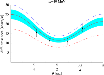
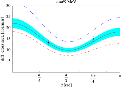
Figure 4: The differential cross section for elastic $\gamma$-deuteron Compton scattering at incident photon energies of $E_{\gamma}=49\ \mathrm{MeV}$ and $69\ \mathrm{MeV}$ in EFT(KSW) [3], no free parameters. Dashed: LO; long dashed: NLO without the graphs that contribute to the nucleon polarisability; solid curve: complete NLO result. The estimate of the accuracy of the calculation at NLO ($\pm 10\%$) is indicated by the shaded area.

Compton scattering has also been investigated in ENT(Weinberg) [14] and in ENT(${\pi\hskip-5.50003pt/}$) [15]. Surprisingly, the results all agree within the theoretical uncertainty of the calculations even at relatively high momenta. This seems to suggest that non-analytic pion contributions from meson exchange diagrams are small.

2.2 Three Body Forces and the Triton

Since all interactions permitted by the symmetries must be included into the Lagrangean, EFT dictates that in the three body sector, interactions like

$$\mathcal{L}_{\mathrm{3body}}=H\;(N^{\dagger}N)^{3}$$ (4)

with unknown strength $H$ are present. Turning again to ENT(${\pi\hskip-5.50003pt/}$), we therefore have to ask at which order in the power counting they will start to contribute. Bedaque, Hammer and van Kolck [16] found the surprising result that an unusual renormalisation makes the three body force of leading order in the triton channel.

In order to understand this finding, let us first consider the LO diagrams which come from two nucleon interactions. The absence of Coulomb interactions in the $\mathrm{nd}$ system ensures that only properties of the strong interactions are probed. All graphs involving only ${}^{\pi\hskip-2.79996pt/}C_{0}$ interactions are of the same order and form a double series which cannot be written down in closed form. Summing all “bubble-chain” sub-graphs into the deuteron propagator, one can however obtain the solution numerically from the integral equation pictorially shown in Fig. 5 within seconds on a personal computer.

(50,50) i2,i1 o2,o1 double,tension=6i1,v1,v2 vanilla,width=thinv2,o1 double,tension=6v3,v4,o2 vanilla,width=thini2,v3 vanilla,width=thinv2,v3 $+$ (80,50) i2,i1 o2,o1 double,tension=4i1,v1 vanilla,width=thinv1,v2 double,tension=4o1,v2 vanilla,width=thini2,v3 vanilla,width=thinv3,o2 vanilla,width=thinv2,v3 vanilla,width=thinv3,v1 $+$ (110,50) i2,i1 o2,o1 double,tension=8i1,v1 vanilla,width=thinv1,v2 double,tension=8o1,v2 double,tension=100v3,v3a double,tension=100v4,v4a phantomv3a,v4a vanilla,width=thini2,v3 vanilla,width=thinv4,o2 vanilla,width=thinv2,v4 vanilla,width=thinv3,v1 vanilla,width=thin,left=0.65v3a,v4a vanilla,width=thin,left=0.65v4a,v3a $+$ (110,50) i2,i1 o2,o1 double,tension=8i1,v1 vanilla,width=thinv1,v4 double,tension=100v4,v5 vanilla,width=thin,tension=1.666v5,o1 double,tension=8o2,v6 vanilla,width=thinv6,v3 double,tension=100v3,v2 vanilla,width=thin,tension=1.666v2,i2 vanilla,width=thinv1,v2 vanilla,width=thinv3,v4 vanilla,width=thinv5,v6 $+\;\dots$

(90,50) i2,i1 o2,o1 double,width=thin,tension=3i1,v1 double,width=thin,tension=1.5v1,v3,v2 double,width=thin,tension=3v2,o1 vanilla,width=thini2,v4,o2 ellipse,rubout=1v3,v4   $=$   (90,50) i2,i1 o2,o1 double,width=thin,tension=4i1,v1,v2 vanilla,width=thinv2,o1 double,width=thin,tension=4v3,v4,o2 vanilla,width=thini2,v3 vanilla,width=thinv2,v3   $+$   (170,50) i2,i1 o2,o1 double,width=thin,tension=3i1,v1 double,width=thin,tension=1.5v1,v6,v5 double,width=thin,tension=3v5,v2 vanilla,width=thinv2,o1 vanilla,width=thini2,v7 vanilla,width=thin,tension=0.666v7,v4 double,width=thin,tension=4v4,v3,o2 vanilla,width=thinv4,v2 ellipse,rubout=1v6,v7

Figure 5: The double infinite series of LO “pinball” diagrams, some of which are shown in the first line, is equivalent to the solution of the Faddeev equation of the second line.

Because one nucleon is exchanged in the intermediate state, each diagram is of the order of the nucleon propagator, i.e. $Q^{-2}$, while the first three buddy force (4) seems to be of order $Q^{0}$. We are therefore tempted to assume that three body forces are at worst N2LO, i.e. of the order $10\%$. In the quartet channel, power counting suggests even N4LO because the Pauli principle forbids three body forces without derivatives. However, such naïve counting was already fallacious in the two body sector because of the presence of a low lying bound state and of a linear divergence in each of the bubble graphs making up Fig. 1. We therefore investigate more carefully the UV behaviour of the amplitude $\mathcal{A}(k,p)$ at half off-shell momenta $p\gg k,\gamma$. The integral equation simplifies then to

$$\mathcal{A}_{(l,s)}(0,p) = \frac{4\;\lambda(s)}{\sqrt{3}\,\pi}\int\limits_{0}^{\infty}\frac{\mathrm{d}q}{p}\;\mathcal{A}_{(l,s)}(0,q)\;Q_{l}\left[\frac{p}{q}+\frac{q}{p}\right]\;\;,$$ (5)

where $\lambda(s)=-\frac{1}{2}$ in the spin quartet channel, and $1$ in the doublet. $Q_{l}$ is the Legendre Polynomial of the second kind, $l$ the angular momentum of the partial wave investigated.

The equation is easily solved by a Mellin transformation, $\mathcal{A}_{(l,s)}(0,p)=p^{-1+s_{0}(l,s)}$, and indeed in most channels $s_{0}$ is real so that only one solution exists which vanishes at infinite momentum and hence is cut-off independent. However, the fact that the kernel of (5) is not compact makes one suspicious whether this is always the case. Indeed, there exists one and only one partial wave in which two linearly independent solutions are found: the doublet $\mathrm{S}$ wave (triton) channel, where $s_{0}(l=0,s=\frac{1}{2})=\pm 1.0062\dots\mathrm{i}$. Therefore in this channel, any superposition with an arbitrary phase $\delta$ is also a solution, and we find that

$$\mathcal{A}_{l=0,s=\frac{1}{2}}(k\to 0,p)\propto\frac{\cos[1.0062\ln p+\delta]}{p}\;\;.$$ (6)

Because each value of the phase provides a different boundary condition for the solution of the full integral equation Fig. 5, the on-shell amplitude $\mathcal{A}(k,p=k)$ will also depend crucially on $\delta$. This means that the on-shell amplitude seems sensitive to off-shell physics, and what is more, to a phase which stems from arbitrarily high momenta. A numerical study of the full half off-shell amplitude confirms these findings, Fig. 6. This cannot be.

Because physics must be independent of the cut-off chosen, this sensitivity of the on-shell amplitude on UV properties of the solution to (5) must be remedied by adding a counter term. And since the power counting in the two nucleon sector is fixed, one can show that a necessary and sufficient condition to render cut-off independent results is to promote the three body force (4) to LO, $H(\delta)\sim Q^{-2}$, and absorb all phase dependence into it, see Fig. 7. The variation of $H(\delta)$ with the cut-off or phase is known analytically from (6), but its initial value is unknown. Therefore, one physical scale $\bar{\delta}$ must be determined experimentally. This one, new free parameter explains why potential models which provide an accurate description of $\mathrm{NN}$ scattering can vary significantly in their predictions of the triton binding energy $B_{3}$ and three body scattering length $a_{3}^{(1/2)}$ in the triton channel, although all of them lie on a curve in the $(B_{3},a_{3}^{(1/2)})$ plane, known as the Phillips line, Fig. 6. Determining $H(\bar{\delta})$ by fixing the three body scattering length to its physical value, the triton binding energy is found in ENT(${\pi\hskip-5.50003pt/}$) to be $8.0\;\mathrm{MeV}$ at LO.

Figure 6: Left: Variation of the cut-off by a factor 3 in a numerical study of the naïve off-shell amplitude Fig. 5 in the triton channel has a dramatic effect on the scattering length $a(p=0)$. Right: Comparison of the ENT prediction for the Phillips line with results from various potential models. Figures from Ref. [16].

$\mbox{\parbox{57.20032pt}{ \fmfgraph*(104,64) \fmfleft{i2,i1} \fmfright{o2,o1} \fmf{double,width=thin,tension=3}{i1,v1} \fmf{double,width=thin,tension=1.5}{v1,v3,v2} \fmf{double,width=thin,tension=3}{v2,o1} \fmf{vanilla,width=thin}{i2,v4,o2} \fmffreeze\fmffreeze\fmf{ellipse,rubout=1}{v3,v4} }}=\mbox{\parbox{57.20032pt}{ \fmfgraph*(104,64) \fmfleft{i2,i1} \fmfright{o2,o1} \fmf{double,width=thin,tension=4}{i1,v1,v2} \fmf{vanilla,width=thin}{v2,o1} \fmf{double,width=thin,tension=4}{v3,v4,o2} \fmf{vanilla,width=thin}{i2,v3} \fmffreeze\fmf{vanilla,width=thin}{v2,v3} }}+\mbox{\parbox{57.20032pt}{ \fmfgraph*(104,64) \fmfleft{i2,i1} \fmfright{o2,o1} \fmf{double,width=thin}{i1,v,o1} \fmf{vanilla,width=thin}{i2,v,o2} \fmfv{decor.shape=circle,decor.filled=full,decor.size=2thick, label=${H(\delta)}$,label.angle=90,label.dist=0.5h}{v} }}+\mbox{\parbox{105.60059pt}{ \fmfgraph*(192,64) \fmfleft{i2,i1} \fmfright{o2,o1} \fmf{double,width=thin,tension=3}{i1,v1} \fmf{double,width=thin,tension=1.5}{v1,v6,v5} \fmf{double,width=thin,tension=3}{v5,v2} \fmf{vanilla,width=thin}{v2,o1} \fmf{vanilla,width=thin}{i2,v7} \fmf{vanilla,width=thin,tension=0.666}{v7,v4} \fmf{double,width=thin,tension=4}{v4,v3,o2} \fmffreeze\fmffreeze\fmf{vanilla,width=thin}{v4,v2} \fmf{ellipse,rubout=1}{v6,v7} }}+\mbox{\parbox{105.60059pt}{ \fmfgraph*(192,64) \fmfleft{i2,i1} \fmfright{o2,o1} \fmf{double,width=thin,tension=3}{i1,v1} \fmf{double,width=thin,tension=1.5}{v1,v6} \fmf{phantom,width=thin,tension=1.5}{v6,v5} \fmf{phantom,width=thin,tension=3}{v5,v2} \fmf{phantom,width=thin}{v2,o1} \fmf{vanilla,width=thin}{i2,v7} \fmf{phantom,width=thin,tension=0.666}{v7,v4} \fmf{phantom,width=thin,tension=4}{v4,v3,o2} \fmffreeze\fmffreeze\fmf{vanilla,width=thin}{v7,v,o2} \fmf{double,width=thin}{v6,v,o1} \fmfv{decor.shape=circle,decor.filled=full,decor.size=2thick, label=${H(\delta)}$,label.angle=90,label.dist=0.5h}{v} \fmf{ellipse,rubout=1}{v6,v7} }}$

Figure 7: The cut-off independent Faddeev equation in the triton channel.

It must again be stressed that the three body force of strength $H(\delta)$ was added not out of phenomenological needs. It cures the arbitrariness in the off-shell and UV behaviour of the two body interactions which would otherwise contaminate the on-shell amplitude. Just as the off-shell behaviour of the two body amplitude Fig. 5, the strength $H(\delta)$ is arbitrary, and only the sum of two and three body graphs is physically meaningful.

Summing the deuteron bubbles, each graph in the upper line of Fig. 5 behaves like $p^{-2}$ in the UV. But the solution of the Faddeev equation goes like $p^{-1+s_{0}}$ with irrational (or even complex) $s_{0}(l,s)$ [17] and is hence more than the naïve sum of graphs.

The limit cycle thus encountered in the triton channel is a new renormalisation group phenomenon and also explains the Efimov and Thomas effects [2, 16]. However, the phenomenon occurs only in the triton channel. In all other partial waves, three body forces enter only at higher orders [17].

2.3 Partial Waves in Neutron–Deuteron Scattering

In the three body sector, the equations to be solved in ENT(${\pi\hskip-5.50003pt/}$) and ENT(KSW) are computationally trivial and can furthermore be improved systematically by higher order correction which involve only (partially analytic, partially numerical) integrations, in contradistinction to many-dimensional integral equations arising in other approaches. A comparative study between the theory with explicit, perturbative pions (ENT(KSW)) and the one with pions integrated out was performed [4] in the spin quartet $\mathrm{S}$ wave for momenta of up to $300\;\mathrm{MeV}$ in the centre-of-mass frame ($E_{\mathrm{cm}}\approx 70\;\mathrm{MeV}$). As seen above, the two formulations are identical at LO. Because three body forces enter only at high orders, this channel is completely determined by two body properties at the first few orders and no new, free parameters enter.

The calculation with/without explicit pions to NLO/N2LO shows convergence: For example, the scattering length is $a({}^{4}S_{\frac{3}{2}},\mathrm{LO})=(5.1\pm 1.5)\;\mathrm{fm}$, and at NLO with (without) perturbative pions $a({}^{4}S_{\frac{3}{2}},\mathrm{NLO,KSW})=(6.8\pm 0.7)\;\mathrm{fm}$ ($a({}^{4}S_{\frac{3}{2}},\mathrm{NLO},{\pi\hskip-5.50003pt/})=(6.7\pm 0.7)\;\mathrm{fm}$). At N2LO, [16] report $a({}^{4}S_{\frac{3}{2}},\mathrm{N2LO},{\pi\hskip-5.50003pt/})=(6.33\pm 0.1)\;\mathrm{fm}$, and the experimental value is $a({}^{4}S_{\frac{3}{2}},\mathrm{exp})=(6.35\pm 0.02)\;\mathrm{fm}$. Comparing the NLO correction to the LO scattering length provides one with the familiar error estimate at NLO: $(\frac{1}{3})^{2}\approx 10\%$. The NLO calculations with and without pions lie within each other’s error bar. The N2LO calculation is inside the error ascertained to the NLO calculation and carries itself a theoretical uncertainty of about $(\frac{1}{3})^{3}\approx 4\%$. The calculation of pionic corrections in ENT(KSW) shows that they are – although formally NLO – indeed much weaker. The difference to ENT(${\pi\hskip-5.50003pt/}$) should appear for momenta of the order of $m_{\pi}$ and higher because of non-analytic contributions of the pion cut, but those seem to be very moderate, see Fig. 8. This and the lack of data makes it difficult to assess whether the KSW power counting scheme to include pions as perturbative increases the range of validity over the pion-less theory.

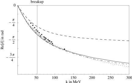
Figure 8: Real parts of the quartet $\mathrm{S}$ [4] and doublet $\mathrm{D}$ [5] wave phase shifts in $\mathrm{nd}$ scattering. Legend left: Dashed: LO; solid (dot-dashed) line: NLO with perturbative pions (pions integrated out); dotted: N2LO without pions. Realistic potential models: squares, crosses, triangles. Stars: $\mathrm{pd}$ phase shift analysis.

Finally, the real and imaginary parts of the higher partial waves $l=1,\dots,4$ in the spin quartet and doublet channel were found [5] in a parameter-free calculation, see Fig. 8. Within the range of validity of this pion-less theory, convergence is good, and the results agree with potential model calculations (as available) within the theoretical uncertainty. That makes one optimistic about carrying out higher order calculations of problematic spin observables like the nucleon-deuteron vector analysing power $A_{y}$ where EFT will differ from potential model calculations due to the inclusion of three-body forces.

3 Outlook

Many questions remain open: Does the power counting Nature chose include pions perturbatively or non-perturbatively? At the moment, some people advocate a mixture. To investigate processes with pions in the initial or final state might be helpful [18]. How to extend the analysis in the triton channel systematically to higher orders? Technically, how to regularise a Faddeev equation numerically with external currents coupled in a field theory? How do four body forces scale? Extend to nuclear matter!

References

- [1] U. van Kolck, M. Savage and R. Seki, eds., “Nuclear Physics with Effective Field Theory”, Proceedings of the INT-Caltech Workshop at Caltech (1998), World Scientific; P. Bedaque, U. van Kolck, M. Savage and R. Seki, eds., “Nuclear Physics with Effective Field Theory II”, Proceedings of the INT-Caltech Workshop at the INT (1999), World Scientific.
- [2] S.R. Beane, P.F. Bedaque, W.C. Haxton, D.R. Phillips and M.J. Savage, nucl-th/0008064.
- [3] J.-W. Chen, H.W. Grießhammer, M.J. Savage and R.P. Springer, Nucl. Phys. A644, 221 (1998); Nucl. Phys. A644, 245 (1998).
- [4] P.F. Bedaque and H.W. Grießhammer, Nucl. Phys. A671, 357 (2000).
- [5] F. Gabbiani, P.F. Bedaque and H.W. Grießhammer, Nucl. Phys. A675, 601 (2000).
- [6] B.R. Holstein, these proceedings.
- [7] E. Epelbaum, these proceedings.
- [8] S. Weinberg, Nucl. Phys. B363, 3 (1991).
- [9] J.-W. Chen, G. Rupak and M.J. Savage, Nucl. Phys. A653, 386 (1999).
- [10] H.D. Politzer, Nucl. Phys. B172, 349 (1980); C. Arzt, Phys. Lett. B342, 189 (1995).
- [11] D.B. Kaplan, M.J. Savage and M.B. Wise, Phys. Rev. C59, 617 (1999).
- [12] D.B. Kaplan, M.J. Savage and M.B. Wise, Phys. Lett. B424, 390 (1998); D.B. Kaplan, M.J. Savage and M.B. Wise, Nucl. Phys. B534, 329 (1998).
- [13] U. van Kolck, Nucl. Phys. A645, 273 (1999).
- [14] S.R. Beane, M. Malheiro, D.R. Phillips and U. van Kolck, Nucl. Phys. A656, 367 (1999).
- [15] H.W. Grießhammer, G. Rupak and M.J. Savage, in preparation.
- [16] P.F. Bedaque, H.W. Hammer and U. van Kolck, Phys. Rev. Lett. 82, 463 (1999); P.F. Bedaque, H.W. Hammer and U. van Kolck, Nucl. Phys. A646, 444 (1999); P.F. Bedaque, H.W. Hammer and U. van Kolck, Nucl. Phys. A676, 357 (2000).
- [17] H.W. Grießhammer, in preparation.
- [18] B. Borasoy and H.W. Grießhammer, in preparation.