^⋆Section for Theoretical and Computational Physics, Department of Physics
University of Bergen, Allegaten 55, 5007 Bergen, Norway
^† KFKI Research Institute for Particle and Nuclear Physics
P.O.Box 49, 1525 Budapest, Hungary
^‡ Theory Division, Los Alamos National Laboratory,
Los Alamos, NM, 87454, USA

A model for energy, pressure and flow velocity distributions at the beginning of relativistic heavy ion collisions is presented, which can be used as initial condition for hydrodynamical calculations. The results show that QGP forms a tilted disk, such that the direction of the largest pressure gradient stays in the reaction plane, but deviates from both the beam and the usual transverse flow directions. Such initial condition may lead to the creation of ”antiflow” or ”third flow component” [10].

 

Introduction. Fluid dynamical models are widely used to describe ultra-relativistic heavy ion collisions. Their advantage is that one can vary flexibly the Equation of State (EoS) of the matter and test its consequences on the reaction dynamics and outcome. In energetic collisions of large heavy ions, especially if Quark-Gluon Plasma (QGP) is formed in the collision, one-fluid dynamics is a valid and good description for the intermediate stages of the reaction. Here, interactions are strong and frequent, so that other models, (e.g. transport models, string models, etc., assuming binary collisions, with free propagation of constituents between collisions) have limited validity. On the other hand, the initial and final, Freeze-Out (FO), stages of the reaction are outside the domain of applicability of the fluid dynamical model.

In conclusion, the realistic, and detailed description of an energetic heavy ion reaction requires a Multi Module Model, where the different stages of the reaction are each described with suitable theoretical approaches. It is important that these Modules are coupled to each other correctly: on the interface, which is a 3 dimensional hyper-surface in space-time with normal $d\sigma^{\mu}$, all conservation laws should be satisfied (e.g. $[T^{\mu\nu}d\sigma_{\nu}]=0$), and entropy should not decrease, $[S^{\mu}d\sigma_{\mu}]\geq 0$. These matching conditions were worked out and studied for the matching at FO in detail in refs. [1].

The final FO stages of the reaction, after hadronization, can be described well with kinetic models where the matter is already dilute.

The initial stages are more problematic. Frequently two or three fluid models are used to remedy the difficulties, and to model the process of QGP formation and thermalization. [2, 3, 4] Here, the problem is transferred to the determination of drag-, friction- and transfer- terms among the fluid components, and a new problem is introduced with the (unjustified) use of EoS in each component in a nonequilibrated situations, where EoS does not exist. Strictly speaking this approach can only be justified for mixtures of noninteracting ideal gas components. Similarly, the use of transport theoretical approaches assuming dilute gases with binary interactions is questionable, as due to the extreme Lorentz contraction, in the C.M. frame, enormous particle and energy densities, with the immediate formation of perturbative vacuum should be handled. Even in most parton cascade models these initial stages of the dynamics are just assumed in form of some initial condition, with little justification behind.

Our goal in the present work is to construct a model, based on the recent experiences gained in string Monte Carlo models and in parton cascades. One important conclusion of heavy ion research in the last decade is that standard ’hadronic’ string models fail to describe heavy ion experiments.

All string models had to introduce new, energetic objects: string ropes [5, 8], quark clusters [6], fused strings [7], in order to describe the abundant formation of massive particles like strange antibaryons. Based on this, we describe the initial moments of the reaction in the framework of classical (or coherent) Yang-Mills theory, following ref. [9] assuming larger field strength (string tension) than in ordinary hadron-hadron collisions. In addition we now satisfy all conservation laws exactly, while in ref. [9] infinite projectile energy was assumed, and so, overall energy and momentum conservation was irrelevant. We do not solve simultaneously the kinetic problem leading to parton equilibration, but assume that the arising friction is such that the heavy ion system will be an overdamped oscillator, i.e. yo-yoing of the two heavy ions will not occur. This assumption is based on recent string and parton cascade results.

 

Formulation of model. Our basic idea is to generalize the model developed in [9], for collisions of two heavy ions and improve it by strictly satisfying conservation laws. First of all, we would create a grid in $[x,y]$ plane ($z$ – is the beam axes, $[z,x]$ – is reaction plane). We will describe the nucleus-nucleus collision in terms of steak-by-streak collisions, corresponding to the same transverse coordinates, $\{x_{i},y_{j}\}$. We assume that baryon recoil for both target and projectile arise from the acceleration of partons in an effective field $F^{\mu\nu}$, produced in the interaction. Of course, the physical picture behind this model should be based on chromoelectric flux tube or string models, but for our purpose we consider $F^{\mu\nu}$ as an effective abelian field. Phenomenological parameters describing this field must be fixed from comparison with experimental data.

Let describe the streak-streak collision.

$$\partial_{\mu}\sum_{i}T_{i}^{\mu\nu}=\sum_{i}F_{i}^{\nu\mu}n_{i\mu}\ ,$$ (1)

$$\partial_{\mu}\sum_{i}n_{i}^{\mu}=0\ ,\quad i=1,2\ ,$$ (2)

$n_{i}^{\mu}$ is the baryon current of $i$th nucleus (we are working in the Center of Rapidity Frame (CRF), which is the same for all streaks. The concept of using target and projectile reference frames has no advantage any more). We will use the parameterization:

$$n_{i}^{\mu}=\rho_{i}u_{i}^{\mu}\ ,\quad u_{i}^{\mu}=(\cosh y_{i},\ \sinh y_{i})\ .$$ (3)

$T^{\mu\nu}$ is a energy-momentum flux tensor. It consists of five parts, corresponding to both nuclei and free field energy (also divided into two parts) and one defines the QGP perturbative vacuum.

$$T^{\mu\nu}=\sum_{i}T_{i}^{\mu\nu}+T^{\mu\nu}_{pert}=\sum_{i}\left[e_{i}\left(\left(1+c_{0}^{2}\right)u_{i}^{\mu}u_{i}^{\nu}-c_{0}^{2}g^{\mu\nu}\right)+T_{F,i}^{\mu\nu}\right]+Bg^{\mu\nu}\ ,\quad i=1,2\ .$$ (4)

$B$ – is the bag constant, the equation of state is $P_{i}=c_{0}^{2}e_{i}$, where $e_{i}$ and $P_{i}$ are energy density and pressure of QGP.

In complete analogy to electro-magnetic field

$$F_{i}^{\mu\nu}=\partial^{\nu}A_{i}^{\mu}-\partial^{\mu}A_{i}^{\nu}=\left(\begin{array}[]{cc}0&-\sigma_{i}\\ \sigma_{i}&0\end{array}\right)\ \ ,$$ (5)

$$\sigma_{i}=\partial^{3}A_{i}^{0}-\partial^{0}A_{i}^{3}\ ,$$ (6)

$$T_{F,i\mu\nu}=-g_{\mu\nu}{\cal L}_{F,i}+\sum_{\beta}\frac{{\cal L}_{F,i}}{\partial\left(\partial^{\mu}A_{i}^{\beta}\right)}\partial_{\nu}A_{i}^{\beta}\ \ ,$$ (7)

$${\cal L}_{F,i}=-\frac{1}{4}F_{i\mu\nu}F_{i}^{\mu\nu}\ .$$ (8)

In our case the string tensions, $\sigma_{i}$, will have the same absolute value $\sigma$ and opposite sign (in complete analogy to the usual string with two ends moving in opposite directions), and $\sigma_{i}$ will be constant in the space-time region after string creation and before string decay.

To get the analytic solutions of the above equations, we use light cone variables

$$(z,t)\rightarrow(x^{+},x^{-}),\quad x^{\pm}=t\pm z\ .$$ (9)

Following [9], we insist that $e_{1},y_{1},\rho_{1},A_{1}^{\mu}$ are functions of $x^{-}$ only and $e_{2},y_{2},\rho_{2},A_{2}^{\mu}$ depend on $x^{+}$ only.

In terms of light cone variables:

$$n_{i}^{\pm}=n_{i,\mp}=\rho_{i}(u_{i}^{0}\pm u_{i}^{3})=\rho_{i}e^{\pm y_{i}}\ ,$$ (10)

$$\left(\begin{array}[]{cc}T_{i}^{++}&T_{i}^{+-}\\ T_{i}^{-+}&T_{i}^{--}\end{array}\right)=\left(\begin{array}[]{cc}h_{i+}e^{2y_{i}}&h_{i-}\\ h_{i-}&h_{i+}e^{-2y_{i}}\end{array}\right)+T_{F,i}\ ,$$ (11)

where

$$h_{i+}=(1+c_{0}^{2})e_{i}\ ,\quad h_{i-}=(1-c_{0}^{2})e_{i}\ .$$ (12)

$$\left(\begin{array}[]{cc}F_{i}^{++}&F_{i}^{+-}\\ F_{i}^{-+}&F_{i}^{--}\end{array}\right)=\left(\begin{array}[]{cc}0&2\sigma_{i}\\ 2\sigma_{i}&0\end{array}\right)\ .$$ (13)

$$T_{pert}=\left(\begin{array}[]{cc}0&2B\\ 2B&0\end{array}\right)\ .$$ (14)

At the time of first touch of two streaks, $t=0$, there is no string tension. We assume that strings are created, i.e. the sting tension achieves the value $\sigma$ at time $t=t_{0}$, corresponding to complete penetration of streaks through each other.

 

Conservation laws — String rope creation. In light cone variables eq. (2) may be rewritten as

$$\partial_{-}n_{1}^{-}+\partial_{+}n_{2}^{+}=0\ .$$ (15)

So, we have a sum of two terms, depending on different independent variables, and the solution can be found in the following way.

$$\begin{array}[]{ll}\partial_{-}n_{1}^{-}=a,&\partial_{+}n_{2}^{+}=-a\ ,\\ n_{1}^{-}=ax^{-}+(n_{1})_{0},&n_{2}^{+}=-ax^{+}+(n_{2})_{0}\ .\end{array}$$ (16)

Since both $n_{1}^{-}$ and $n_{2}^{+}$ are positive (and also more or less symmetric) we can conclude that for our case $a=0$.

Finally

$$n_{1}^{-}=\rho_{1}e^{-y_{1}}=\rho_{0}e^{y_{0}}\ ,\quad n_{2}^{+}=\rho_{2}e^{y_{2}}=\rho_{0}e^{y_{0}}\ ,$$ (17)

$$\rho_{1}=\rho_{0}e^{y_{0}+y_{1}}\ ,\quad\rho_{2}=\rho_{0}e^{y_{0}-y_{2}}\ .$$ (18)

Let us come back to the energy-momentum tensor $T^{\mu\nu}$. Based on eqs. (6, 7, 8) and taking into account the Lorentz gauge, $\partial^{0}A_{i}^{0}-\partial^{3}A_{i}^{3}=0$, we can find

$$\left(\begin{array}[]{cc}T_{F,i}^{++}&T_{F,i}^{+-}\\ T_{F,i}^{-+}&T_{F,i}^{--}\end{array}\right)=\left(\begin{array}[]{cc}\sigma_{i}^{2}-2\sigma_{i}\left(\partial^{0}A_{i}^{0}\right)+2\sigma_{i}\left(\partial^{3}A_{i}^{0}\right)&0\\ 0&\sigma_{i}^{2}+2\sigma_{i}\left(\partial^{0}A_{i}^{0}\right)+2\sigma_{i}\left(\partial^{3}A_{i}^{0}\right)\end{array}\right)\ .$$ (19)

As mentioned before, after string creation, i.e. $t>t_{0}$, and before string decay we choose the string tensions in the form:

$$\sigma_{2}=-\sigma_{1}=\sigma>0\ .$$ (20)

To satisfy the above choice and the Lorentz gauge condition we take the vector potentials in the following form:

$$\begin{array}[]{ll}A_{1}^{+}=0,&A_{1}^{-}=-2\sigma x^{-}\ ,\\ A_{2}^{+}=-2\sigma x^{+},&A_{2}^{-}=0\ .\end{array}$$ (21)

In our calculations we used the parameterization:

$$\sigma=A\left(\frac{\varepsilon_{0}}{m}\right)^{2}\rho_{0}\sqrt{l_{1}l_{2}}\ ,$$ (22)

where $l_{1},\ l_{2}$ are the lengths of initial streaks. The typical values of $A$ are around $0.05-0.06$. Notice, that there is only one free parameter in parameterization (22). The typical values of $\sigma$ are $8-15\ GeV/fm$ for $\varepsilon_{0}=100\ GeV/nucl$.

The problem with eq. (1) is that we do not know what the really conserved quantities are. Using the definition of $F^{\mu\nu}$, eq. (6), we can rewrite eq. (1) as

$$\partial_{\mu}T^{\mu\nu}=\sum_{i}F_{i}^{\mu\nu}n_{i,\mu}=\sum_{i}\left(\partial^{\mu}\left(A_{i}^{\nu}n_{i,\mu}\right)-A^{\nu}\partial^{\mu}n_{i,\mu}-\partial^{\nu}\left(A_{i}^{\mu}n_{i,\mu}\right)+A^{\mu}\partial^{\nu}n_{i,\mu}\right)\ .$$ (23)

The solution for $n_{1}^{-}$ and $n_{2}^{+}$, eq. (17), shows as that second and fourth terms vanish. So, we can define new energy-momentum tensor $\tilde{T}^{\mu\nu}$, such that

$$\partial_{\mu}\tilde{T}^{\mu\nu}=0\ ,$$ (24)

$$\tilde{T}^{\mu\nu}=\sum_{i}\tilde{T_{i}}^{\mu\nu}+T^{\mu\nu}_{pert}=\sum_{i}\left(T_{i}^{\mu\nu}-A_{i}^{\nu}n_{i}^{\mu}+g^{\mu\nu}A_{i}^{\alpha}n_{i\alpha}\right)+Bg^{\mu\nu}$$ (25)

Using the exact definition of $A_{i}^{\mu}$ – eqs. (21) – we obtain

$$\tilde{T}^{\mu\nu}=\left(\begin{array}[]{cc}h_{1+}e^{2y_{1}}+5\sigma^{2}&h_{1-}+4\sigma x^{-}n_{1}^{+}\\ h_{1-}+2\sigma x^{-}n_{1}^{+}&h_{1+}e^{-2y_{1}}+\sigma^{2}-2\sigma x^{-}n_{1}^{-}\end{array}\right)+\left(\begin{array}[]{cc}h_{2+}e^{2y_{2}}+\sigma^{2}+2\sigma x^{+}n_{2}^{+}&h_{2-}-2\sigma x^{+}n_{2}^{-}\\ h_{2-}-4\sigma x^{+}n_{2}^{-}&h_{2+}e^{-2y_{2}}+5\sigma^{2}\end{array}\right)$$

$$+\left(\begin{array}[]{cc}0&2B\\ 2B&0\end{array}\right)\ .$$ (26)

Now the new conserved quantities are

$$Q_{0}=\int\tilde{T}^{00}dV=\sum_{i}\int_{\Omega_{i}}\tilde{T_{i}}^{00}dV\ ,$$ (27)

$$Q_{3}=\int\tilde{T}^{03}dV=\sum_{i}\int_{\Omega_{i}}\tilde{T_{i}}^{03}dV\ .$$ (28)

Based on conservation of $Q_{0},\ Q_{3}$ we can calculate rapidity, energy and baryon densities at the moment $t=t_{0}$, when the string with tension $\sigma$ is created. These new quantities are used as initial conditions for our differential eqs. (1, 2).

$$\left(\frac{\varepsilon_{1}(t_{0})}{m}\right)=\left(\frac{\varepsilon_{0}}{m}\right)\frac{1}{1{+}c_{0}^{2}}-\frac{\sigma^{2}}{\rho_{0}\varepsilon_{0}(1{+}c_{0}^{2})}\frac{l_{1}{+}5l_{2}}{4l_{1}}-\frac{\sigma e^{y_{0}}}{8\varepsilon_{0}(1{+}c_{0}^{2})}(l_{1}{+}2l_{2})-\frac{B}{\rho_{0}\varepsilon_{0}(1{+}c_{0}^{2})}\frac{l_{1}{+}l_{2}}{2l_{1}}\ ,$$ (29)

$$\left(\frac{\varepsilon_{2}(t_{0})}{m}\right)=\left(\frac{\varepsilon_{0}}{m}\right)\frac{1}{1{+}c_{0}^{2}}-\frac{\sigma^{2}}{\rho_{0}\varepsilon_{0}(1{+}c_{0}^{2})}\frac{l_{2}{+}5l_{1}}{4l_{2}}-\frac{\sigma e^{y_{0}}}{8\varepsilon_{0}(1{+}c_{0}^{2})}(l_{2}{+}2l_{1})-\frac{B}{\rho_{0}\varepsilon_{0}(1{+}c_{0}^{2})}\frac{l_{1}{+}l_{2}}{2l_{2}}\ .$$ (30)

Here the $\varepsilon_{i}$ is energy per nucleon in CRF. Now the proper baryon density can be found, $\rho_{i}(t_{0})=\rho_{0}\frac{\varepsilon_{0}}{\varepsilon_{i}(t_{0})}$, $\gamma_{i}=\frac{1}{\sqrt{1-v_{i}^{2}}}=\frac{\varepsilon_{i}(t_{0})}{m}$.

For $x^{\pm}>x_{0}$, where $x_{0}=2t_{0}-|z(0)|$ defines the string creation surface $t=t_{0}$, for nucleon or cell element in the position $z=z(0)$ at the time $t=0$, we should solve eqs. (24), with boundary conditions

$$\begin{array}[]{ll}n_{1}^{\pm}(x^{-}=x_{0})=\rho_{0}e^{\mp y_{0}}&n_{2}^{\pm}(x^{+}=x_{0})=\rho_{0}e^{\pm y_{0}}\\ &\\ h_{1+}(x^{-}=x_{0})=e_{1}(t_{0})(1+c_{0}^{2})&h_{2+}(x^{+}=x_{0})=e_{1}(t_{0})(1+c_{0}^{2})\\ &\\ y_{1}(x^{-}=x_{0})=y_{1}(t_{0})&y_{2}(x^{+}=x_{0})=y_{2}(t_{0})\\ &\\ \sigma_{1}(x^{-}=x_{0})=-\sigma&\sigma_{2}(x^{+}=x_{0})=\sigma\ ,\end{array}$$ (31)

where $e_{i}(t_{0})=m\rho_{i}(t_{0})$ – energy density in the rest frame of $ith$ nuclei.

Let us present the complete analytical solution in the following form

$$e^{(-)^{i+1}2y_{i}}=-\frac{d_{i}}{b_{i}}+\left(\frac{d_{i}}{b_{i}}+e^{(-)^{i+1}2y_{i}(t_{0})}\right)\left(1-\frac{x^{i}-x_{0}}{\tau_{i}}\right)^{-\frac{b_{i}}{\alpha a_{j}}}\ ,$$ (32)

$$h_{i+}=e^{(-)^{i+1}2y_{i}}e_{i}(t_{0})(1+c_{0}^{2})e^{-(-)^{i+1}2y_{i}(t_{0})}\left(1-\frac{x^{i}-x_{0}}{\tau_{i}}\right)\ ,$$ (33)

$$\rho_{i}=\rho_{0}e^{y_{0}}e^{(-)^{i+1}y_{i}}\ ,$$ (34)

where $x^{1}=x^{-},\ x^{2}=x^{+}$, $i,j=1,2\ ,\ i\not=j$,    and using the notations

$$b_{i}=\alpha a_{j}+2\sigma\rho_{0}e^{y_{0}}\ ,$$ (35)

$$d_{i}=c_{i}-2\sigma\rho_{0}e^{y_{0}}e^{(-)^{i+1}2y_{i}(t_{0})}\ ,$$ (36)

$$\tau_{i}=\frac{e_{i}(t_{0})(1+c_{0}^{2})}{e^{(-)^{i+1}2y_{i}(t_{0})}a_{j}}\ ,$$ (37)

$$a_{1}=c_{1}+2\sigma\rho_{0}e^{y_{0}}-2\sigma\rho_{0}e^{y_{0}}e^{2y_{1}(t_{0})}\ ,\quad a_{2}=c_{2}+2\sigma\rho_{0}e^{y_{0}}-2\sigma\rho_{0}e^{y_{0}}e^{-2y_{2}(t_{0})}\ ,$$ (38)

$$c_{i}=\alpha((1+c_{0}^{2})e_{i}(t_{0})-e_{0})/2t_{0}\ .$$ (39)

Then the trajectories of nucleons (or cell elements) for both nuclei are given by:

$$\begin{array}[]{c}x_{1}^{+}(x^{-})=z(0)+\int_{t_{0}}^{x^{-}}dx\ e^{2y_{1}(x)}=\\ \\ z(0)-\frac{d_{1}}{b_{1}}(x^{-}-x_{0})+\left(\frac{d_{1}}{b_{1}}+e^{2y_{1}(t_{0})}\right)\tau_{1}\frac{\alpha a_{2}}{2\sigma\rho_{0}e^{y_{0}}}\left[\left(1-\frac{x^{-}-x_{0}}{\tau_{1}}\right)^{-\frac{2\sigma\rho_{0}e^{y_{0}}}{\alpha a_{2}}}-1\right]\ ,\end{array}$$

$$\begin{array}[]{c}x_{2}^{-}(x^{+})=-z(0)+\int_{t_{0}}^{x^{+}}dx\ e^{-2y_{2}(x)}=\\ \\ -z(0)-\frac{d_{2}}{b_{2}}(x^{+}-x_{0})+\left(\frac{d_{2}}{b_{2}}+e^{-2y_{2}(t_{0})}\right)\tau_{2}\frac{\alpha a_{1}}{2\sigma\rho_{0}e^{y_{0}}}\left[\left(1-\frac{x^{+}-x_{0}}{\tau_{2}}\right)^{-\frac{2\sigma\rho_{0}e^{y_{0}}}{\alpha a_{1}}}-1\right]\ ,\end{array}$$

for nucleon or cell element in the position $z=z(0)$ at the time $t=0$.

 

Recreation of the matter. As we may see from the trajectories, eqs. (, ), nucleons (or cell domains) will keep going in the initial direction up to the time $t=t_{i,turn}$, then they will turn and go backwards until the two streaks again penetrate through each other and new oscillation will start. Such a motion is analogous to the ”Yo-Yo” motion in the string models. Of course, it is difficult to believe that such a process would really happen in heavy ion collisions, because of string decays, string-string interactions, interaction between streaks and other reasons, which are quite difficult to take into account. To be realistic we should stop the motion described by eqs. (, ) at some moment before the projectile and target cross again.

We assume that the final result of collisions of two streaks after stopping the string’s expansion and after its decay, is one streak with length $\bigtriangleup l_{f}$, homogeneous energy density distribution, $e_{f}$, and baryon charge distribution, $\rho_{f}$, moving like one object with rapidity $y_{f}$. We assume that this is due to string-string interactions and string decays. As it was mentioned above the typical values of the string tension, $\sigma$, are of the order of $10\ GeV/fm$, and these may be treated as several parallel strings. The string-string interaction will produce a kind of ”string rope” between our two streaks, which is responsible for final energy density and baryon charge homogeneous distributions. Now it is worth to mention that decay of our ”string rope” does not allow charges to remain at the ends of the final streak, as it would be if we assume full transparency.

The homogeneous distributions are the simplest assumptions, which may be modified based on experimental data. Its advantage is a simple expression for $e_{f},\ \rho_{f},\ y_{f}$.

The final energy density and rapidity, $e_{f}$ and $y_{f}$, may be determined from conservation laws.

$$\cosh^{2}y_{f}=\frac{(M^{2}(1+c_{0}^{2})+2c_{0}^{2})+\sqrt{(M^{2}(1+c_{0}^{2})+2c_{0}^{2})^{2}+4c_{0}^{4}(M^{2}-1)}}{2(1+c_{0}^{2})(M^{2}-1)}\ ,$$ (40)

where we neglected $B\bigtriangleup l_{f}$ next to $Q_{0}$ and introduced the notation $M=(l_{2}+l_{1})/(l_{2}-l_{1})$,

$$e_{f}=\frac{{Q_{0}\over\bigtriangleup x\bigtriangleup y}-B\bigtriangleup l_{f}}{((1+c_{0}^{2})\cosh^{2}y_{f}-c_{0}^{2})\bigtriangleup l_{f}}\ .$$ (41)

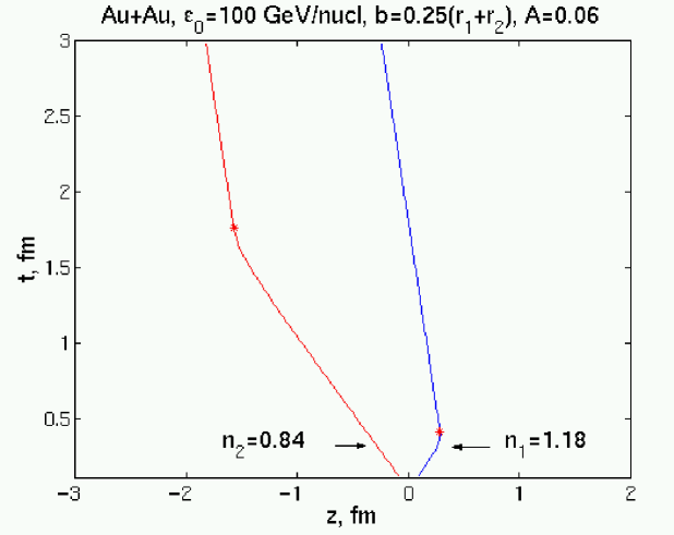
Figure 1: The typical trajectory of the ends of two initial streaks, corresponding to numbers of nucleons, $n_{1}$ and $n_{2}$. Stars denote the stopping and turning points, where $y_{i}=y_{f}$. From $t_{0}$ to the turning points streak ends keep going in their initial direction according to eqs. (, ). Later the final streak starts to move like one object with rapidity, $y_{f}$ (40) in CRF.

The typical trajectory of the streak ends is presented in Fig. 1. From $t_{0}$ they move according to eqs. (, ) until they reach the rapidity $y_{i}=y_{f}$. Later the final string starts to move like one object with rapidity $y_{f}$.

The turning points can be found from the condition:

$$y_{i}=y_{f}\ ,$$ (42)

which gives for $i$th nucleus ($x_{1}=x^{-},\ x_{2}=x^{+}$)

$$x_{i,\ turn}=x_{0}+\tau_{i}\left[1-\left(\frac{\frac{d_{i}}{b_{i}}+e^{(-)^{i+1}2y_{i}(t_{0})}}{\frac{d_{i}}{b_{i}}+e^{(-)^{i+1}2y_{f}}}\right)^{\frac{\alpha a_{j}}{b_{i}}}\right]\ .$$ (43)

 

Initial conditions for hydrodynamical calculations. In this section we present the results of our calculations. We are interested in the shape of QGP formed, when string expansions stop and their matter is locally equilibrated. This will be the initial state for further hydrodynamical calculations. We may see in Figs. 2, that QGP forms a tilted disk for $b\not=0$. So, the direction of fastest expansion, the same as largest pressure gradient, will be in the reaction plane, but will deviate from both the beam axis and the usual transverse flow direction. So, the new flow component, called ”antiflow” or ”third flow component”, will appear in addition to the usual transverse flow component in the reaction plane. With increasing beam energy the usual transverse flow is getting weaker, while this new flow component is strengthened. The mutual effect of the usual directed transverse flow and this new ”antiflow” or ”third flow component” lead to an enhanced emission in the reaction plane. This was actually observed and widely studies earlier and referred to as ”elliptic flow”.

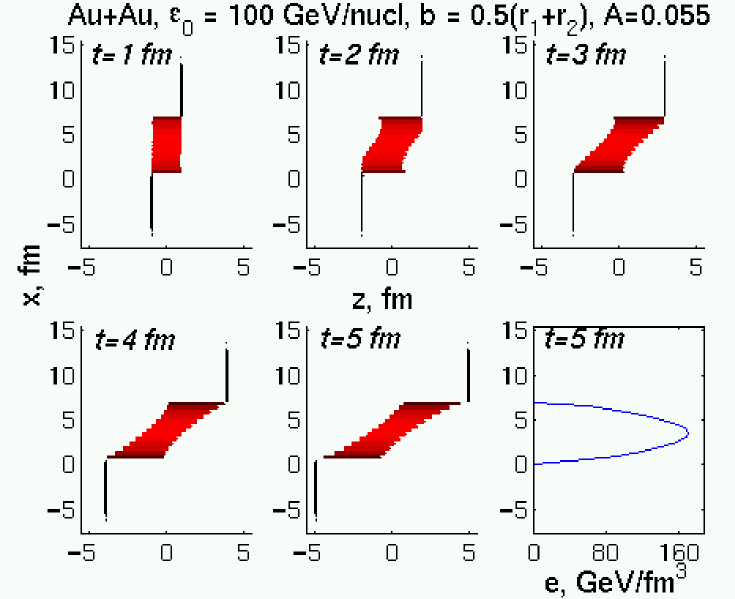
Figure 2: The Au+Au collisions, $\varepsilon_{0}=100\ GeV/nucl$, $b=0.5(R_{1}+R_{2})$, $A=0.055$ (parameter $A$ introduced in (22)), $y=0$ (ZX plane through the centers of nuclei). We would like to notice that final shape of QGP volume is a tilted disk $\approx 45^{0}$, and the direction of the fastest expansion will deviate from both the beam axis and the usual transverse flow direction, and might be a reason for the third flow component, as argued in [10].

 

Conclusions. Based on earlier Coherent Yang-Mills field theoretical models, and introducing effective parameters based on Monte-Carlo string cascade and parton cascade model results, a simplified model is introduced to describe the pre fluid dynamical stages of heavy ion collisions at the highest SPS energies and above. The model predicts limited transparency for massive heavy ions.

Contrary to earlier expectations, — based on standard string tensions of 1 GeV/fm which lead to the Bjorken model type of initial state, — effective string tensions are introduced for collisions of massive heavy ions, as a consequence of collective effects related to QGP formation. These collective effects in central and semi central collisions lead to an effective string tension of the order of 10 GeV/fm and consequently cause much less transparency than earlier estimates. The resulting initial locally equilibrated state of matter in semi central collisions takes a rather unusual form, which can be then identified by the asymmetry of the caused collective flow. Our prediction is that this special initial state may be the cause of the recently predicted ”antiflow” or ”third flow component”.

Detailed fluid dynamical calculations as well as flow experiments at semi central impact parameters for massive heavy ions are needed at SPS and RHIC energies to connect the predicted special initial state with observables.

References

• [1] V.K. Magas, Cs. Anderlik, L.P. Csernai, F. Grassi, W. Greiner, Y. Hama, T. Kodama, Zs. Lázár and H. Stöker, (nucl-th/9808024),  Phys. Rev. C59 (1999) 388; (nucl-th/9806004),  Phys. Rev. C59 (1999) 3309; (nucl-th/9903045),  HIP 9 (1999) 193; (nucl-th/9905054),  Phys. Lett. B 459 (1999) 33.
• [2] A.A. Amsden et al.,  Phys. Rev. C17 (1978) 2080.
• [3] L.P. Csernai et al.,  Phys. Rev. C26 (1982) 149.
• [4] J. Brachmann, S. Soff, A. Dumitru, H. Stöker, J.A. Maruhn, W. Greiner, D.H. Rischke, L. Bravina,  Phys. Rev. C61 (2000) 024909.
• [5] T.S. Biro, H.B. Nielsen, J. Knoll,  Nucl. Phys. B245 (1984) 449.
• [6] K. Wegner, J. Aichelin,  Phys. Rev. Lett. 76 (1996) 1027.
• [7] N.S. Amelin, M.A. Braun, C. Pajares,  Phys. Lett. B306 (1993) 312,  Z. Phys. C63 (1994) 507.
• [8] H. Sorge,  Phys. Rev. C52 (1995) 3291.
• [9] M. Gyulassy, L.P. Csernai,  Nucl. Phys. A460 (1986) 723.
• [10] L.P. Csernai, D. Röhrich, nucl-th/9908034,  Phys. Lett. B458 (1999) 454.