Microscopic model approaches to fragmentation of nuclei and phase transitions in nuclear matter

Abstract

The properties of excited nuclear matter and the quest for a phase transition which is expected to exist in this system are the subject of intensive investigations. High energy nuclear collisions between finite nuclei which lead to matter fragmentation are used to investigate these properties. The present report covers effective work done on the subject over the two last decades. The analysis of experimental data is confronted with two major problems, the setting up of thermodynamic equilibrium in a time-dependent fragmentation process and the finite size of nuclei. The present status concerning the first point is presented. Simple classical models of disordered systems are derived starting with the generic bond percolation approach. These lattice and cellular equilibrium models, like percolation approaches, describe successfully experimental fragment multiplicity distributions. They also show the properties of systems which undergo a thermodynamic phase transition. Physical observables which are devised to show the existence and to fix the order of critical behaviour are presented. Applications to the models are shown. Thermodynamic properties of finite systems undergoing critical behaviour are advantageously described in the framework of the microcanonical ensemble. Applications to the designed models and to experimental data are presented and analysed. Perspectives of further developments of the field are suggested.

PACS: 25.70Pq, 64.60Ak, 64.60Fr, 05.70Ce, 05.70Jk, 05.50+q

Key words: Nuclear fragmentation, phase transitions, lattice models, cellular models.

e-mail:
¹richert@lpt1.u-strasbg.fr
²pierre.wagner@ires.in2p3.fr

1 Introduction

Protons and neutrons are able to form bound nuclei with well defined lifetimes. They are finite and contain a relatively small number of nucleons which varies from one to several hundreds. The nucleons experience a strong short range interaction which acts together with the long range Coulomb interaction between the charged protons. The interactions between nucleons determine the ground state properties and the low energy excitation spectrum of nuclei which have been studied over several decades. Their description by means of very different collective and microscopic, semi-classical and quantum models has lead to a satisfactory understanding of their properties [1, 2, 3].

With increasing excitation energy the detailed information coded in the spectrum and the wave functions of the system gets less and less meaningful and stringent for a satisfactory description of the system. Statistical arguments get relevant. Random matrix theories, for instance, have proved to be a very efficient tool in this regime [4, 5]. Under certain circumstances experiments reveal that the behaviour of nuclei can be described in the framework of thermodynamics. Excited nuclei behave like equilibrated compounds which may decay through emission of gamma rays, nucleons or light clusters at energies corresponding to unbound states of the system [6]. The behaviour of nuclei in this regime and its description in terms of thermodynamic and statistical concepts leads to intriguing questions related to the general properties of thermodynamically equilibrated nuclear matter, either finite like nuclei or (quasi)infinite as it could be found in neutron stars, in the absence of the gravitational interaction. These questions are also triggered by the fact that nucleons are fermions and nuclear matter in its ground state, at zero temperature, shows the properties of a Fermi liquid of strongly interacting particles [7, 8, 9, 10]. For high enough excitation energy it seems sensible to think that such a quantum liquid may go over to a quantum gas by undergoing a phase transition which would be observable in a infinite system and for which one would find characteristic signals in finite nuclei.

This question has become a major source of interest over the last two decades in the nuclear physics community. The only way to get an experimental answer to it goes through energetic collisions between nuclei or nucleons and nuclei with the aim to generate excited finite nuclear matter. The analysis of the experiments must then be able to reveal its properties and eventually deliver signs for the existence of one or several phase transitions in the infinite system.

Such ambitious objectives have led to intense experimental and theoretical investigations. Several reports have been written on the subject over the last ten years. In the present review we aim to discuss two aspects concerning excited nuclear matter. The first concerns the conditions under which it is experimentally generated. The second deals with specific microscopic models which we think allow a realistic study and description of experimental facts under the prerequisite that the physical conditions imposed by the experiment match those which are imposed by the theory.

The content of the present review is the following. In section 2 we describe the status of the subject at the beginning of the early 80’s. We present and discuss the attempts to interpret experimental results related to energetic heavy ion collisions and the theoretical models which were aimed to describe the outcome of such collisions, the fragmentation of the involved nuclei. We then turn over in section 3 to the two major points which have to be taken in account in order to be able to compare experimental results with the type of models which will be introduced. These points concern the finiteness of the system and the problems related to its properties with respect to the concept of thermodynamic equilibrium. Section 4 is devoted to the outcome of very energetic nuclear collisions. Nuclei can break up into pieces. Fragments with different sizes, mass and charge numbers, are generated. With the presently available detection instruments they can be recorded. Their charge and, to some extent, their mass can be measured. Charge and mass distributions as well as related quantities are a priori non-trivial observables which contain interesting information about the fragmentation process and the behaviour of excited nuclear matter. We present and discuss the concepts and models which have been introduced in order to describe the fragmentation characteristics of nuclei, as well as the possible reasons for which rather simple-minded models describe these observables with a remarkable success. In section 5 we introduce microscopic statistical models which may behave as generic approaches for the study of the thermodynamic properties of excited systems composed of interacting nucleons. These models have either been borrowed from other fields of physics or consist of adapted derivatives of these models. They describe systems which show phase transitions and whose outcome can be confronted with experimental data. Since they are finite, tests which enable to characterize the phase transitions have been proposed. Some of these tests are introduced in section 6 and their application both on theoretical models as well as experimental results are presented and discussed in the perspective of the existence of a phase transition in excited nuclear matter. In section 7 we develop a summary, comment the present status of the field and suggest perspectives which may lead to further progress in the field.

Nuclear fragmentation and the search of phase transitions is a very active field of research. This is best seen by looking at the number of preprints and publications which appear regularly. We tried to cover the newest results concerning the aspects of the subject with which the present report is concerned, extending to summer 2000. We also tried to be as exhaustive as possible in the presentation and quotation of the work which has been done. We apologize for the contributions which could have been forgotten because of lack of information about their existence.

2 Properties of excited nuclei and nuclear matter : first experimental and theoretical attempts

Finite nuclei in their ground state and low-lying excited states have been studied for over 50 years. They are still objects of interest, in particular the so called exotic nuclei which contain a larger number of protons or neutrons than those which lie in the so called valley of stability. These objects can be conceptually considered as finite representatives of infinite nuclear matter which may be realized in large objects of our universe like neutron stars where nucleons experience of course both the nuclear and gravitational interactions, the last one being absent from our present considerations.

Extensive theoretical studies of the ground state properties of infinite nuclear matter have been pursued over several decades. They were essentially aimed to determine the non relativistic nucleon-nucleon interaction which originates from meson exchanges between nucleons. Its precise expression can be fixed by means of nucleon-nucleon scattering amplitudes [11, 12, 13, 14, 15]. Different expressions of this interaction have been introduced in order to construct effective interactions used in detailed spectroscopic studies of the ground state and low excited states of nuclei, see f.i. refs. [16, 17].

At high enough excitation energy, nuclei which form liquid drops of fermions get unstable. It is tempting to trace a parallel with the behaviour of macroscopic liquids and to conjecture that the nuclear liquid may go over into vapour and that there may exist a transition from a liquid to a gas under precise thermodynamic conditions, in the limit of an infinite system. But this is not necessarily the case, the evolution with increasing energy could well correspond to a smooth crossover from a bound to an unbound system of interacting particles. The question whether nuclear matter may exist in different phases is one of the important questions raised by the nuclear community and a central point of the present review. The first serious attempts to answer this question started about two decades ago.

2.1 Critical phenomena in nuclear matter : experimental facts and early interpretations

2.1.1 Fragmentation of nuclei

Experimental information about excited nuclear matter can only be gained through accelerator induced nuclear reactions by means of which excited nuclei can be generated and studied. Energetic beams of particles or heavy ions shot on nuclei lead to their fragmentation into pieces. The final multiplicity of fragments of different sizes which are collected by the detectors is correlated with the degree of violence of the collision. To our knowledge, the first experiment which was concerned with the possible observation of signs related to a phase transition in nuclei was performed in 1982 by Minich et al. [18]. Protons with energies between 80 and $350\,GeV$ were shot on xenon and krypton targets. The resulting experimentally detected fragments with $A$ nucleons $(12\leq A\leq 31)$ and $Z$ protons led to fragment yields $Y(A,Z)$ which could be parametrized in the form

$$Y(A,Z)\propto A^{-\tau}f(A,Z,T)$$ (1)

where $\tau$ is a positive exponent and $f(A,Z,T)$ a Boltzmann factor which depends on a temperature $T$ and further constants which were fixed by a fit procedure to the experimental data. Expression (1) was in fact inspired by Fisher’s droplet model [19] which for the pupose of the analysis was generalized to two types of particles, neutrons and protons. The value of the critical exponent extracted from the fit of the data was $\tau=2.64$ and 2.65 for xenon and krypton respectively. It has to be compared to the value $\tau=2.33$ obtained in mean field theory [20]. Fisher’s condensation theory predicts that the transition from a liquid to a gas proceeds via the formation of droplets whose size distribution follows a power law at the critical transition point. The authors do not claim that these results would be a proof for the existence of a critical behaviour but that they are consistent with it. Following the droplet model, the increase in excitation energy would generate instabilities in nuclear matter and would lead, at some critical temperature $T_{c}$, to the disassembly of the system, which is here finite, into smaller pieces of all sizes which are experimentally detected.

This pioneering experiment has been prolongated in further work which was pursued by Panagiotou et al. [21, 22]. The authors introduced a systematic study of twelve different high energy reactions induced by protons and carbon ions on Ag, Kr, Xe and U targets. They measured fragment yields corresponding to nuclei with $3\leq Z\leq 22$. Using the same point of view as in ref. [19] the yields of fragments of size $A$ were parametrized in the explicit form

$$P(A) \propto A^{-k}\exp\{[-a_{s}(T)A^{2/3}-a_{v}(T)A+\mu(T)A]/T\}$$

$$= A^{-k}X^{A^{2/3}}Y^{A}$$

where

$$X=\exp[-a_{s}(T)/T]$$

and

$$Y=\exp[-(a_{v}(T)-\mu(T))/T]$$

Here $T$ is the temperature of the fragmenting system, $a_{s},a_{v},\mu$ are the surface, volume free energy per particle and the chemical potential respectively. $T$ was determined independently for the different systems by different means [21]. Under the assumption that there exists a critical temperature $T_{c}$ at which $a_{s}(T)$ vanishes, the different quantities were further parametrized as

$$a_{s}(T) = 18.4(1-T/T_{c})^{2}$$

$$a_{v}(T)-\mu(T) = b(1-T/T_{c})^{2}$$

where $b$ is a coefficient which has to be fixed. For $T<T_{c}$ where the gas and liquid coexist

$$a_{v}(T)-\mu(T)=0$$

$$\textrm{hence }Y=1$$

at $T=T_{c}$. Furthermore

$$a_{s}(T_{c})=0$$

$$\textrm{hence }X=1$$

For $T>T_{c}$ one assumes that $a_{s}(T)\simeq 0$.

The expression $P(A)$ was fitted to the experimental data in order to fix $b$ and $T_{c}$, for different values of $k$ (=1.6 - 2.33) and in a temperature range $T^{\prime}=T\pm 1$ where $T$ is the supposed common temperature of all emitted fragments. The values of $T$ were chosen within an interval of $2\,MeV$ in order to take the uncertainty related to this quantity in account. If one fixes the critical temperature to the lowest value of $\tau(T)$ in a parametrization $P(A,T)\propto A^{-\tau(T)}$ where $\tau$ is a so called apparent exponent, then the fitted value of $T_{c}$ coincides for $1.7\leq k\leq 1.8$ with $T_{c}\simeq 12\,MeV$. Further analysis of the same type [22] confirmed these results, i.e. a critical temperature which lies in the range 9.5 - 13.5 $MeV$ and an exponent $k$ smaller than 2.

2.1.2 Thermodynamic interpretation of fragment yields : comments and discussions

The model which is aimed to reproduce the outcome of the fragmentation reactions presented above presupposes that the process can be described in the framework of thermodynamics and the grand canonical ensemble. It assumes that the fragmenting system is in thermodynamic equilibrium. This assumption is strong since it implies that there exists a relaxation time which is not longer than the time interval which separates the beginning of the process and the time at which fragments are formed. We shall come back to this point at different places below.

The system undergoes a phase transition at a characteristic temperature $T_{c}$. For $T<T_{c}$ a gas and a liquid coexist. The liquid phase is made of particles and composite droplets (fragments) whose energy is composed of a volume and a surface contribution. At $T=T_{c}$ the surface contribution disappears, the droplets disassemble into independent nucleons, hence form an homogeneous gas phase which is reached for $T>T_{c}$.

Taking the problem of thermal equilibrium apart, further thinking about this attractive picture leads to the following comments. First, the data analysis is restricted to a finite range in the size of fragments. Light and heavy species are not taken in account. This may introduce a bias which is not under control. It has to be noticed that the exponents $\tau$ and $k$ which were obtained in refs. [21] and [22] do not coincide with the exponent expected from the Fisher model which describes classical and infinite systems. Finite size effects should play a role in the determination of critical exponents, here they are not taken in account. Finally fragments and particles are free, i.e. they do not interact with each other. Even if the nuclear interaction is weak at the fragmentation stage because the system has already expanded, the Coulomb energy is present and certainly non negligible. Hence it should be taken into account.

At this stage, even though there were encouraging signs for the existence of a critical behaviour of nuclear matter, it appeared that the observed phenomenon was not reducible to an ordinary liquid-gas phase transition as described by Fisher’s droplet model. However, these first steps and the concepts they introduced paved the way to a huge amount of theoretical work which we shall briefly describe below, as far as the existence of different phases is concerned.

2.2 Microscopic interpretations

Here we restrict ourselves to those approaches which have been introduced as stationary and non-stationary descriptions of finite excited systems. They were aimed to describe the response and fate of nuclei when energy is imparted to them.

2.2.1 Temperature-dependent Hartree-Fock approaches

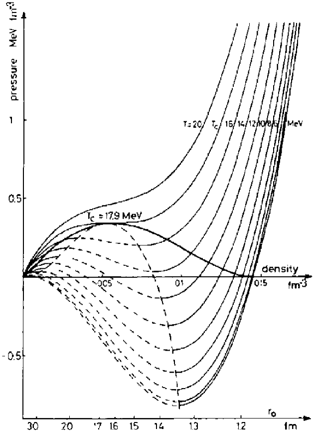
Figure 1: Equation of state relating the pressure to the density in nuclear matter [25]. The curves represent isotherms. The spinodal region is indicated by dashed curves.

The droplet model [19] is a classical and phenomenological description of an excited, inhomogeneous and unstable matter phase. The most common approximation introduced in the framework of the quantum many-body problem is Hartree-Fock theory in which nucleons move in a self-consistent mean field which can be described by an effective density-dependent interaction. This framework has been used up to the present time for the study of static nuclear properties, a detailed review of its applications can be found f.i. in [23] and references therein. The theory has been extended to the study of systems at finite temperature in the framework of the canonical and grand canonical ensembles [24, 25, 26, 27, 28, 29]. Using point contact and density-dependent effective interactions like Skyrme interactions it is easy to derive explicit expressions of different equations of state such as the expression of the pressure $P$ as a function of the density $\rho$ for different values of the temperature $T$. The typical behaviour of these quantities is presented in Fig. 1. One observes the existence of an area limited by an envelope, the spinodal line, where the pressure decreases with increasing density. This is the signal for the presence of an instability of matter which corresponds to the formation of an inhomogeneous medium. It is interpreted as a zone where liquid and gas coexist and which is not thermodynamically accessible. The transition from an homogeneous to the unstable regime corresponds to a first order phase transition in the thermodynamic limit. The transition is of second order at the critical point corresponding to the critical temperature $T_{c}$, at the maximum of the spinodal line where $\mathrm{d}^{2}P/\mathrm{d}\rho^{2}=0$. This behaviour establishes a connection with the droplet model physics. Condensation has been studied in this framework [20]. The calculations fix the critical density $\rho_{c}$ and the critical temperatures. The presence and importance of the Coulomb interaction was first taken into account by Levit and Bonche [30] who introduced a description in which the system is composed of a bound, excited nucleus surrounded by an external gas made of light particles in thermal equilibrium with the nucleus. The presence of the long range Coulomb force produces a sizable qualitative effect. It results in the apparition of a so called limiting temperature, $T_{lim}$, which restricts the instability zone to temperatures which are lower than $T_{c}$ and hence introduces an important modification. Similar investigations were performed in refs. [31, 32] with different Skyrme interactions and refinements concerning, in particular, the treatment of the vapour charge.

The temperature-dependent Hartree-Fock approach with density-dependent effective interactions is a simple and elegant approximation to the many-body problem of finite excited systems. A priori it is possible to find the correspondence with central ingredients of the droplet model like the concept of surface in the liquid phase. It is however difficult to control the degree of realism of these microscopic quantum approaches. The fact that the process is described in the framework of the canonical or grand canonical ensemble when the fragmenting system is closed and has a fixed and small number of particles may lead to difficulties in the characterization of the transition. We shall come back to this point in the sequel. There are no means to obtain fragment yields which could be compared to the experiment since there are only two types of species, a bound nucleus and light particles which constitute respectively the liquid and the vapour phases. This is of course directly related to a major difficulty which comes from the mean field description. The phases are homogeneous. Many-body correlations induced by the neglected residual two-body interactions are absent, but their effect is very important at the considered excitation energies. This may also explain the high values of the temperature $T_{c}\simeq 15-20\,MeV$ where the system becomes unstable. Indeed, the interpretation of experiments indicates that these temperatures could be much lower, of the order of $4-6\,MeV$.

Hence this kind of approach is at most indicative for the determination of the properties of finite excited nuclear matter in thermodynamic equilibrium. It worked however as an incentive to develop more realistic approaches which take explicitly care of the many-body aspect of the problem. We describe some of them below.

2.2.2 Time-dependent descriptions of nuclear fragmentation

The general microscopic framework describing energetic collisions leading to the decay of the system into species of all sizes is the quantum many-body scattering theory. In this fundamental approach the scattering $S$-matrix elements $S_{fi}$ measure the overlap between any arbitrary many-body initial scattering state $i$ with any arbitrary final state $f$ [33, 34]. A full fledged microscopic approach of this type is however hopelessly out of scope because of its mathematical intricancy. Many pragmatic ways have been devised in order to circumvent this problem. They all rely on non relativistic formalisms in which non nucleonic degrees of freedom are parametrized by means of nucleon-nucleon potentials. All approaches which have been used in a time-dependent framework contain a minimum of classical ingredients. Indeed, all of them fix initial conditions at an initial time and follow the evolution of the system up to a final time in contradistinction with scattering theory which specifies both the initial and the final state of the system.

It is not necessarily clear that classical concepts and assumptions should work in the present physical context, except for the fact that high energy processes are correlated with short wavelengths. One may however notice that processes like deep-inelastic or fission reactions which occur at lower collision energies can be reasonably and surprisingly well reproduced in terms of classical (or semi-classical) equations of motion [35, 36].

An explicit time-dependent description generally called “dynamic” description shows a priori a further advantage, since it allows to avoid the crucial point concerning thermodynamic equilibrium. Indeed, the dynamical description of the evolution of the system may lead or not to thermodynamic equilibrium which follows a transient period of time in a collision process.

There exists essentially two classes of models of this type. The first one transcribes the many-body equations of motion into kinetic equations of motion for the one-particle phase-space distribution function $f(\vec{r},\vec{p},t)$ at point $\vec{r}$ with momentum $\vec{p}$. Each phase space cell $\{[\vec{r},\vec{r}+\mathrm{d}\vec{r}],[\vec{p},\vec{p}+\mathrm{d}\vec{p}]\}$ evolves in time through the transport equation

$$\frac{\partial f}{\partial t}+\frac{\vec{p}}{m}\cdot\frac{\partial f}{\partial\vec{r}}+\frac{\partial V}{\partial\vec{r}}\cdot\frac{\partial f}{\partial\vec{p}}=I[f]$$ (2)

where $V(\vec{r})$ is a one-body potential and $I[f]$, the so called collision term contains in principle all the information relative to $2-,3-,n-$body correlations which are generated by the two-body (possibly also $3-,\ldots,n-$body) potentials beyond the average field $V$. This quantity and $I[f]$ are in principle correlated and fixed in the framework of the initial many-body equation of motion in such a way as to satisfy conservation laws. In practice however they are determined through phenomenological considerations which preserve more or less the quantal aspects of the initial problem. These approximations are particularly tricky for $I[f]$ which has to be chosen in such a way that it can be expressed in terms of one-body distributions, in order to ensure the closed form of (2) [37, 38]. The mean field potential $V$ is generally fixed independently, from purely phenomenological formulations to self-consistent density-dependent expressions derived by means of static Hartree-Fock calculations. As a consequence, a large amount of models of the type of Eq. (2) have been proposed in the litterature, see [37] and refs. therein. They have been used as descriptions of many-body systems, among which high energy nuclear collisions. It is not our aim to give a detailed report on the achievements of these descriptions. It has been done in different publications and reports, see the references above. Here we want to restrict the subject to the discussion of some aspects of nuclear fragmentation which have been addressed in this framework. They are of interest for the understanding of the fragmentation process and problems related to thermodynamic equilibrium, the possible existence and (or) the coexistence of phases in nuclear matter.

In the formulation of Eq. (2) the mean field $V$ plays an essential role and its choice is central for a realistic description of the evolution of the system at high energy. As we have seen in section 2.2.1, realistic mean field calculations in the framework of Hartree-Fock theory with effective density-dependent potentials $V$ and the equation of state $P(\rho)$ lead to a zone of instability and possibly of metastability whose separation from pure “liquid” and “gas” phases corresponds to the existence of a first order phase transition, see Fig. 1. Transport equations may be considered as time-dependent extensions of mean field approaches which furthermore avoid the problem of the existence or not of thermal equilibrium in the expanding and decaying system. Much work has been done in this framework in order to identify the existence and consequences of an instability zone where the initially homogeneous system gets inhomogeneous and appears as formed of clusters which can be identified [39, 40]. This has indeed been achieved in a pure mean field approximation, in the absence of the collision term, when the mean field is supposed to possess a fluctuating contribution [41, 42, 43, 44, 45], and (or) when the collision term induces fluctuations in the one-body distribution function $f(\vec{r},\vec{p},t)$ [46, 47]. These fluctuations develop collective modes like zero sound, some of which are unstable and break the system [48, 49]. The expansion of the system affects also the development of the instabilities. The presence of two types of particles, protons and neutrons has been taken into account [50] and comparisons with experimental results have been made [51]. Quantum effects on the expansion dynamics have been investigated recently. It comes out that they are non negligible, especially when the energy of the collective modes which develop in the system are larger than the temperature [52, 53].

This approach which describes the fragmentation of nuclei as a mechanical process shows however limitations due to the already mentioned fact that Eq. (2) is an approximation to the many-body problem whose expression allows for many more or less controlled phenomenological ingredients, such as stochastic contributions in the mean field and (or) the collision term. These are supposed to simulate the missing many-body features. Unfortunately it is difficult to control their degree of consistency, much physical information is hidden in numerics and may obscure the conclusions which can be drawn from comparisons with the experiment. On the other hand one can believe that transport models of the type given by Eq. (2) are able to describe the time evolution of global observables like inclusive reaction cross sections and collective properties like flow [37].

The second approach concerns molecular dynamics. It is also an approximation to the time-dependent many-body problem. Different formulations starting from the most classical one, Classical Molecular Dynamics (CMD) try to pick up quantal aspects at different levels, going from “Quantum” Molecular Dynamics (QMD) which tries to approximate the many-body wave function at the initial time by means of coherent (gaussian) states and takes care of the Pauli principle [54, 55] to the more recent Fermion Molecular Dynamics (FMD) [56, 57, 58] and Antisymmetrized Molecular Dynamics (AMD) [59, 60, 61, 62] which introduce the antisymmetrization of wave functions in a semi-classical way.

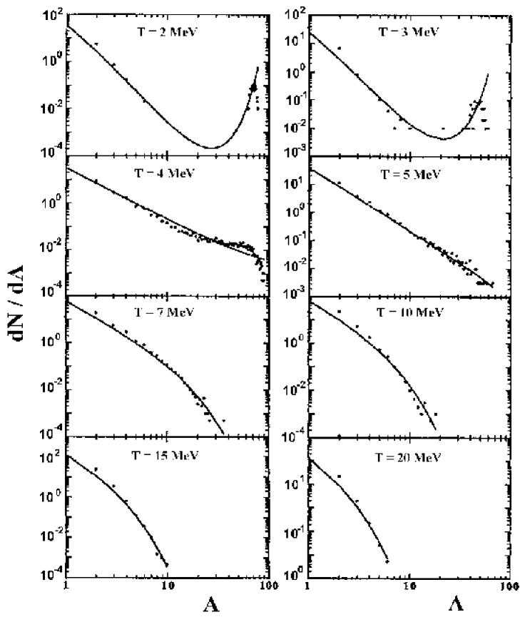
Figure 2: Mass distributions for an expanding system of $A=100$ particles for different initial temperatures [64]. The dots are obtained by means of CMD calculations, the lines are fits using Fisher’s formula.

In the simplest form (CMD) the time evolution of the system is described in terms of classical equations of motion for protons and neutrons which interact through a two-body potential representing the nuclear interaction and the Coulomb force which acts between protons. These interactions are implemented in such a way that the fundamental ground state properties of real nuclei are reproduced. The effects of the Pauli principle can be mimicked by means of a momentum-dependent potential [54]. Applications of this formalism have been developed into different directions. We shall come back in the forthcoming section to the description of heavy ion collisions in which theoretically calculated and experimental determined observables are confronted in order to fix the possible relationship between fragmentation and phases in nuclear matter. Here we concentrate on applications in which Molecular Dynamics (MD) has been implemented in order to study the properties of a thermalized system for which the velocity distributions of particles are maxwellians. From there on the system evolves in time by expansion for different initial values of the temperature and the density [63, 64, 65] One follows the evolution of the temperature, the pressure and the fragment size distribution of the system with decreasing density. Fragments can be identified by means of different criteria which may be more or less realistic [64, 66, 67]. In some cases the system crosses the spinodal line and enters the instability zone. Different observables show a behaviour which can be interpreted in terms of Fisher’s droplet model, i.e. a fragment size distribution corresponding to a power law corrected for finite size effects and a corresponding critical exponent $\tau\simeq$ 2.2 to 2.3, which goes over to other characteristic shapes for other choices of the temperature as expected in the droplet theory, see Fig. 2. These results along with the interpretation of other observables which will be defined below are interpreted as the outcome of a realistic simulation of the experimental situation and the sign for the existence of a critical behaviour of the system. The role and importance of the Coulomb interaction has been investigated [64]. Molecular Dynamics has also been used in order to construct the equation of state [65], i.e. the thermodynamic properties which link density, pressure and temperature. It is again shown that there exists a critical point for finite systems, and a power law distribution with $\tau\simeq 2.23$ which can be interpreted in the framework of Fisher’s model.

However these results and conclusions concerning criticality have been put in question by another study [68] which claims that the observed signs have not to be interpreted as being related to a critical behaviour but for the existence of an intermediate regime. This behaviour would correspond to a trajectory in the $(T,\rho)$ plane on which the evolving system does neither fall back to a drop nor develop into a gas. A power law distribution can be extracted from the data. The power law exponent depends sensitively on the initial temperature and the size of the system. In ref. [68] it is claimed that the power law behaviour of mass yields expected for a system close to its critical point would be purely accidental.

Time-dependent transport descriptions of nuclear fragmentation seem a priori to be the most realistic way to the description of high energy nuclear collisions. They have been widely used in order to describe the possible out-of-equilibrium character of the fragmentation process which characterizes at least the first stage of the process [69]. In the present section we concentrated on aspects related to a time-dependent description of thermodynamically equilibrated systems which expand and cool down, exploring different regions of the $(P,\rho)$ and $(T,\rho)$ planes. Calculations show that the results can be interpreted as the entrance of the system into a thermodynamic unstable regime. It seems however not clear how this can effectively be related to the existence of a phase transition which would characterize an equilibrated system heated up in a fixed volume. In an interpretation in which the system gets critical it is claimed that it is possible to extract critical exponents, at least the power law exponent $\tau$ [63]. However this quantity is obtained from finite size systems and hence should be corrected for finite size effects.

The time coordinate which is introduced in these descriptions raises the question of time scales, i.e. the question concerning equilibration in energetic light particle reactions or heavy ion collisions. This is the subject of section 3. Last but not necessarily least, all these time-dependent approaches need a detailed description of the dynamics in terms of more or less sophisticated mean field and two-body potentials. It is always difficult to get a clear feeling for the sensivity of the outcome of numerical calculations and simulations to these details. Paradoxically, it is at criticality that the information on microscopic systems is the less sensitive to the details of the Hamiltonians which govern them.

Finally it is worthwhile to mention here that it has been shown recently [70] that even far-from-equilibrium, spatially chaotic systems can show equilibrium properties such as ergodicity (equivalence between time and ensemble averages), detailed balance in microscopic processes, partition functions and renormalization group flow at coarse-grained lengths between microscopic and macroscopic scales. This suggests that it might be possible to describe the global behaviour of some far-from-equilibrium systems in the framework of equilibrium statistical mechanisms. Whether this result could be some clue to the actual question raised in the present framework is an open and highly interesting question.

3 Thermodynamic equilibration and phase space descriptions of nuclear fragmentation

If an isolated system of particles is such that there is no unbalanced force acting between its constituents and if it does not experience internal structure changes of its constituents it is said to be in mechanical and chemical equilibrium. Thermal equilibrium is realized if the relevant degrees of freedom which characterize the system share equally its macroscopic energy. One can then define a common temperature which characterizes the energy attributed to each degree of freedom. When all three conditions are realized the system is said to be in thermodynamic equilibrium [71] and can be described in terms of macroscopic coordinates, the thermodynamic coordinates like density, pressure and temperature which do not change with time and are linked together through equations of state. In the present section we aim to present and discuss the difficult and for a large part unsettled problem of thermodynamic equilibrium in small systems like nuclei excited by means of energetic collisions between particles or nuclei called heavy ions if their mass is larger than 4. In section 3.1 we discuss questions related to the interval of time over which equilibrium can be reached in terms of model estimates. A confrontation between experimental facts and phase space equilibrium models is presented in section 3.2.

3.1 Thermodynamic equilibration in excited nuclear systems generated by nuclear collisions

What is the scenario which governs energetic collisions? Data analysis and their interpretation show that several scenarii are at hand. Typically one expects that part of the bombarding energy is transferred to the internal degrees of freedom of the system, the system may fall into pieces, particles and fragments, and expand in time. The remnants are then collected at asymptotic distances in detectors which identify their charges and eventually their masses, along with their kinetic energies and distributions in space. The setting up of thermodynamic equilibrium over the whole or part of the interacting system of particles is a central but open question. Under favorable circumstances one may figure out that after some transient interval of time which starts at the beginning of the collision the system reaches at least partial equilibrium at some stage and then expands to infinity.

3.1.1 Low energy time scales

At very low projectile energies the excitation of nuclei by means of light particles can lead to the formation of an excited complex whose behaviour can be interpreted within the framework of thermodynamics as a system in thermodynamic equilibrium and which can loose part of its excitation energy through the emission of particles, photons or through symmetric or asymmetric fission. The complex is the so called compound nucleus whose formation and decay properties were already studied in the 30’s by N. Bohr [1, 72] who conjectured that, in the framework of this scenario, the process can be explained as a two step mechanism in which the decay of the equilibrated system would be totally uncorrelated from the way it was generated. From a theoretical point of view compound nucleus theory is a phenomenological approach. It has been largely investigated and worked out in terms of microscopic models, among others random matrix theory. There exists an extended litterature on this subject which covers several decades of intensive work [73]. Indeed, the consequences of the model have been abundantly verified by means of physical observables like excitation functions and angular distributions of emitted particles [73, 74]. The lifetime $\tau$ of the compound system can in principle be read from the compound nucleus decay width $\Delta E$ through $\Delta E\cdot\tau\geq\hbar$ leading to $\tau\simeq 10^{-20}-10^{-17}s$ depending in particular on the size of the system. These times are substantially larger than $\tau_{0}\sim\ell/3\times 10^{-23}s$ corresponding to the time necessary to light to cross a nucleus of diameter $\ell\,fm$.

At higher energies, above the Coulomb barrier which corresponds to bombarding energies per particle $E/A\simeq 1-2\,MeV$, reactions involving heavy ions lead to a new mechanism the so called deep inelastic collision (DIC) process. Typical contact times during which the projectile and the target interact through the short range nuclear potential are much shorter than compound nucleus decay times, of the order of $10^{-21}s$, not much larger than the contact time in so called direct reactions in which the ions strike each other peripherally in typical time intervals of $10^{-22}s$. The interpretation of physical observables measured in these DICs shows that although the characteristic reaction times are quite short, the complex which is formed over the contact time of the two ions is sufficient to transfer sizable amounts of energy from the relative motion between ions into the excitation of the nucleonic degrees of freedom and the characteristic features of the system can be interpreted in terms of an equilibrated system whose equilibration is reached in as short as some units of $10^{-22}s$ [35, 75].

3.1.2 Approaches to the equilibration problem at high energies

How does this behaviour extrapolate to high energy events which can lead to the fragmentation of the system into many pieces of different sizes? The problem is intricate since it is difficult to guess the scenario (or the different scenarii) as already mentioned above. Hence one may proceed in steps, starting with simple-minded models. To our knowledge, the first attempt was made by Boal [76], at the time where the experiments, which led to the belief that signs for the existence of a phase transition had been seen, were performed [21, 22]. In fact the question which was raised did not concern the equilibration but the fragment formation time. Former experiments [77] had shown that the ratio between inelastic proton reactions $\sigma(p,p^{\prime})$ and proton-neutron exchange reactions $\sigma(p,n)$, $\sigma(p,p^{\prime})/\sigma(p,n)$, is of the order of 2 at $100\,MeV$ incident energy after correction for the $Z/N$ ratio $(Z,N=$ proton and neutron number). This is evidence for the fact that chemical equilibrium is not reached, hence strictly speaking thermodynamic equilibrium cannot be either, see above. The author of ref. [76] postulates that a hot system generated at high temperature cools down to a fraction of this temperature and, from thereon, experiences particle coalescence leading to the formation of clusters which come out as fragments. Defining $N_{i}(t)$ as the number of clusters of size $i$ which exist at time $t$ normalized to the total number of particles $A_{T}$, the initial conditions are supposed to be given by

$$N_{1}(t=0) = \rho$$

$$N_{i}(t=0) = 0\qquad 2\leq i\leq A_{T}$$

where $\rho$ is the matter density. The system starts at temperature $T$ from an homogeneous distribution of particles and its evolution is given by the postulated rate equations

$$\frac{\mathrm{d}N_{k}(t)}{\mathrm{d}t}=\sum_{i,j}\frac{N_{i}(t)N_{j}(t)}{1+\delta_{ij}}\overline{\sigma_{ij}}\delta_{i+j,k}-\sum_{i}N_{i}(t)N_{k}(t)\overline{\sigma_{ik}}$$ (3)

where the first term on the r.h.s. of (3) corresponds to the coalescence of species of size $i$ and $j$ to species of size $k$ and the second term to the decay of species of size $k$ to species of size $i$. The coalescence and break-up rates are given by

$$\overline{\sigma}=4\pi\bigg{(}\frac{\mu}{2\pi T}\bigg{)}^{3/2}\int\mathrm{d}vv^{3}\sigma(v)\exp(-\mu v^{2}/2T)$$

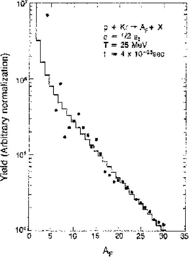
Figure 3: Histogram of mass yields obtained by means of the rate equations (3) after $t=4\times 10^{-23}s$ [76]. The dots are experimental results of the reaction $p+Kr$ at $E=80-350\,GeV$.

where $\mu$ is the reduced mass of the colliding species, $v$ their relative velocity and $\sigma(v)$ the corresponding cross section. The solutions of the system of coupled equations (3) reaches the asymptotic regime after $4\times 10^{-23}s$. The results are shown in Fig. 3 by the histogram for the case of a reaction $p+Kr$ at energies between $80$ and $350\,GeV$. Their global trend agrees quite nicely with the experimental points. The asymptotic time is in agreement with the $\sigma(p,p^{\prime})/\sigma(p,n)$ ratio and the estimated rate of cooling of the excited source, $\sim 10^{-23}s$. One should mention here that the energy is very high and that thermal equilibrium is postulated since one defines a temperature $T$ which is furthermore kept constant over the duration time of the process. The expansion of the system in space is not taken into account. In a further work [78] Boal and Goodman abandoned the coalescence scenario of an initially homogeneous and expanded system. They proposed a break-up mechanism related to the entrance of the system into an instability region of the equation of state as already discussed in section 2. The collision of energetic protons $(E_{p}=300\,MeV)$ with nuclei was simulated by means of a simplified transport equation of the Boltzmann-Uehling-Uhlenbeck (BUU) type. The authors emphasize the fact that thermal equilibrium, requested by a classical collision time between nucleons which is short compared to the expansion time of the nucleon gas, may not be established at a time where the system is already dilute, a regime which is reached after a very short characteristic time which is smaller than $10^{-22}s$. This goes in the same direction as the non equilibrium $\sigma(p,p^{\prime})/\sigma(p,n)$ which was experimentally found. Notice however that the energies involved here are very large, non nucleonic degrees of freedom are not taken into account and the transport description is somewhat schematic. The different models are used in order to explain the increase of entropy of the system when it crosses the spinodal line and enters the instability zone. This entropy agrees with the quantity extracted from the experiment.

Some aspects of fragmentation related to time scales have been discussed by Gross and coll. [79]. The reaction process goes through a transient out-of-equilibrium phase which may ultimately lead to the formation of an equilibrated excited system. In order to estimate the transient time the authors use a BUU-type equation [80, 81, 82, 83] which is a mean field description without collision term as described in section 2. They argue that this description may be valid at the beginning of the collision process, up to and not further than the time when the system may break into pieces. At energies of 50 to $60\,MeV\!\cdot\!A$ this happens after $50-60\,fm/c$ for a reaction ${}^{96}Mo$ on ${}^{96}Mo$. Then the system expands and apparently reaches equilibrium at about $200\,fm/c$ due to the dissipation of energy in the nucleonic degrees of freedom. How far the equilibrium is reached is however not firmly established. Once the distance between the different species gets larger than $3\,fm$, they do no longer interact by means of the nuclear potential. The system has then reached the so called freeze-out stage in which it is in chemical equilibrium. A phase space description of fragments and particles which move under their mutual Coulomb interaction can then be introduced. The early time behaviour is confirmed by experimental results [84].

Recently relativistic transport equations [85] have been used in order to simulate the heavy ion reaction $Au$ on $Au$ which has been studied experimentally [86, 87]. The calculations show that after the collision the excited system separates into a participant region of highly excited matter and a spectator which reaches thermal equilibrium, approximately after $2\cdot 10^{-22}s$. Indeed, a local temperature can be defined through the knowledge of fragment kinetic energies. It characterizes a system which is mechanically unstable and decays into fragments. The values of the temperatures obtained for different beam energies compare well with those which are extracted from the experiments [88, 89].

Other decay scenarii borrowed from low energy reaction mechanisms have been introduced [90, 91, 92, 93, 94, 95]. Fragments are formed sequentially in time, by means of the successive binary decay of the excited species which already exist at a given time step. The process starts from an equilibrated excited system. In ref. [92] this mechanism is supplemented by a boost in time due to the early compression of the system at the beginning of the process. Most of these approaches rely on the Weisskopf formulation of the break-up rates [96] of an excited bound cluster of particles. In ref. [94] the binary decay is interpreted in terms of fission barriers, using a formulation introduced by Swiatecki [97]. The use of the Weisskopf expressions raises problems which shed doubt about their physical relevance at high energies. First, they get unrealistically small at energies corresponding to temperatures above $4-5\,MeV$ [98]. Second [79], each decay event in this formulation should be independent of the preceding one. This is only possible if the characteristic emission time exceeds the characteristic time over which the Coulomb emission barrier changes for the following emission. This time is of the order of $10^{-21}s$, much longer than the Weisskopf emission time and not compatible with characteristic fragment formation times as estimated from the experiments [99]. Hence, although confrontation of mass yields obtained in this framework with experiments may seem satisfactory it is difficult to believe this type of description [100] for highly excited systems. It is of course sensible to believe that fragmentation of nuclei proceeds through a sequence of break-ups, but it is difficult to guess a priori or to derive from some microscopic model the realistic expressions of the rates which govern them when the excitation energy is as high as several $MeV/A$.

The evolution of the fragment emission time has been studied recently by means of two-fragment correlation measurements over a large range of excitation energies in reactions $\pi^{-}$ and $p$ on ${}^{197}Au$ [101]. The fragments are emitted from a unique source which is considered to be in thermal equilibrium. Confrontation of the data with results obtained by means of classical trajectory calculations allows to follow the emission time which decreases with increasing excitation energy. The result is interpreted as evidence for a cross-over from surface emission over long times as described by sequential decay and fast bulk emission which is characteristic of a break-up process due to mechanical instability.

It has also been looked for further direct insight into the time scale problem. In ref. [102] central-impact-parameter events from the reaction ${}^{40}Ar+^{51}V$ with incident energies between 35 and $85\,MeV\!\cdot\!A$ were analysed for the shape of the emitted particle and fragment events in momentum space. It is expected that fragments which are emitted quasi-simultaneously show a close to isotropic emission in the centre of mass system, hence are spherical in shape, whereas emission times which are long as it may be in the case of sequential emission would correspond to the existence of an elongated emission axis, hence an ellipsoidal shape. Experimental events were confronted with numerical simulations. It comes out that for energies below $35\,MeV\!\cdot\!A$ the fragmentation process is slow. For higher energies, the experimental momentum distributions lie in between the predictions corresponding to a slow and a quasi simultaneous break-up process. Even though the result does not give any quantitative clue to the problem, it shows at least that the characteristic fragmentation time decreases with increasing energy. A fragmentation experiment induced by ${}^{40}Ca+^{40}Ca$ at $35\,MeV\!\cdot\!A$ [103] confronted with different models related to quick and slow processes confirms the fact that ordinary binary sequential decay may not be the appropriate fragmentation mechanism.

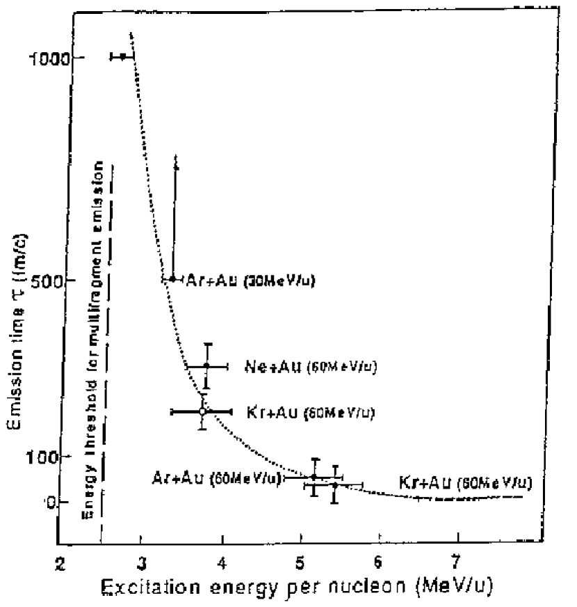
Figure 4: Evolution of the average length of the interval of time between two successive break-ups in the fragmentation process with increasing excitation energy [104].

Other characteristic time scales can be introduced such as the time for the occurence of the first break-up of the system $\tau_{0}$, and the average length of the interval of time between successive break-ups $\tau_{FF}$ [104]. These times can be estimated by means of relative angle correlation measurements between breaking species. If the break-up time is slow, Coulomb repulsion will hinder the emission at small relative angle and low relative velocity. Simulations of the correlation functions indicate that $\tau_{FF}$ corresponds to prompt decay for excitation energies exceeding $4\,MeV/A$. Estimates of $\tau_{FF}$ are shown in Fig. 4. A long time interval $\tau_{0}$ has been observed for excitation energies lower than $3\,MeV/A$ in peripheral collision events. Even for high excitation energies of the order of $5\,MeV/A\$ $\tau_{0}\sim 100-150\,fm/c$. This leads to characteristic times of $300-400\,fm/c$ for complete break-up which are rather large for heavy nuclei, close to the Fermi energy. Recently further emission times have been deduced from IMF-IMF correlation functions obtained from hadron induced multifragmentation events [101]. One observes an evolution from typical emission times $\tau\simeq 500\,fm/c$ at excitation energies $E^{*}/A=2\,MeV$ to $\tau\simeq 20-50\,fm/c$ for $E^{*}/A=5\,MeV$ and above. The observation of the transition is interpreted as a transition from surface to bulk-dominated emission. The characteristic times are somewhat shorter than those obtained in ref. [104, 105] for excitation energies lower than $6\,MeV/A$.

Albeit the numerous and different types of investigations which have been made up to now the arguments concerning a quick thermodynamic equilibration of the system and relying explicitly on time remain the subject of controversies since time is not directly under experimental control. These controversies are in particular raised by time-dependent descriptions of the collision process, in the framework of the Quantum Molecular Dynamics (QMD) models [106, 107, 54]. These are classical molecular dynamics models which, to some extent, take care of the quantum nature of nucleons. In recent applications of this type of models to specific reactions which have been investigated experimentally in some details like ${}^{129}Xe$ on $Sn$ at $50\,MeV\!\cdot\!A$ incident energy, the confrontation between calculations and experimental results shows good quantitative agreement, except for the mass yields corresponding to fragments with more than 30 nucleons and too small kinetic energies for fragments and particles [108]. It is argued that the system of interacting particles is far from equilibrium, there is no sign for a thermally equilibrated behaviour of the species which are generated during the early stages of the process. In a further study [109] QMD calculations are confronted with $50\,MeV\!\cdot\!A$ $Xe+Sn$ data which were also analysed in the framework of the Statistical Multifragmentation Model (SMM, see below) [110]. The approach assumes thermodynamic equilibrium at the freeze-out. Experimental data related to the multiplicities of light charged particles (LCP), the average kinetic energy of LCPs and intermediate mass fragments (IMF) are very close to those obtained by means of QMD and SMM simulations. This result concerning the average transverse kinetic energy of IMFs and the total kinetic energy of LCPs contradicts two arguments which were supposed to help to distinguish between a fragmentation in an equilibrated and non equilibrated system [111].

The preceding discussion shows once more that the experimental data related to fragmentation processes are ambiguous as far as the production mechanism is concerned. It raises the question why the outcome of different descriptions should be so close to each other when the process is over, i.e. at the freeze-out. At the present stage where different models lead to similar results which agree more or less satisfactorily with the experiment it is tempting to conclude that all of them contain part of the truth, at least to a sufficient degree as to agree with the measured quantities. Since there exists no trustful method to settle the point, one has to collect a maximum amount of informations, as exclusive as possible, and confront them directly with theoretical descriptions. In the next subsection we intend to show that in fact most of the data can be understood in terms of systems which reach thermodynamic equilibrium at the freeze-out.

As a final remark, one may wonder why the occupation of phase space leading to equilibrium goes so fast, seemingly even faster at high than at low excitation energy. In a quantum mechanical microscopic description, the decay width of a state $|f\!>$ into a state $|i\!>$ at the energy $E$ is given by the golden rule expression

$$\Gamma(E)\propto 2\pi|V_{fi}|^{2}\rho_{f}(E)$$

where $V_{fi}$ is the interaction matrix element between the initial and final state and $\rho_{f}$ the density of states at the energy of the final state. For increasing energy $E$, $\rho_{f}(E)$ will increase exponentially and if $V_{fi}$ does not decrease as fast as or faster than $\rho_{f}$ which is certainly the case, $\Gamma(E)$ increases with $E$. If we associate a transition time $\tau(E)\propto\hbar/\Gamma(E)$ to this process, one sees that the transition time between different states of the system can decrease very fast and hence drastically accelerate the path to equilibration.

3.2 Thermodynamic equilibrium : confrontation of experimental data with phase space models

Excited nuclei in thermodynamic equilibrium are described by means of so called statistical models. They generally describe a situation where the system is at the freeze-out, the stage at which particles and fragments present in the system are located at relative distances $d$ from each other which are larger than $2-3\,fm$, so that the nuclear interaction between them is negligible. Before we show applications of this type of models to the analysis of experimental results we present and discuss some of their aspects.

3.2.1 The first phase space models

To our knowledge, the first attempts to describe strongly excited systems of particles and bound clusters were made in the beginning of the 80’s. The concept of statistical multifragmentation was first introduced in ref. [112]. In 1981, Randrup and Koonin proposed a thermodynamic phase space model [113]. They defined the partition function $\mathcal{Z}$ of a classical system in the grand canonical ensemble in which the number of particles $A$, $N$ neutrons and $Z$ protons, as well as the energy, is fixed in the average. If $A_{0}$ is the average number of particles, one defines

$$\omega=\ln\mathcal{Z}/A_{0}=\sum_{AT}\omega_{\scriptscriptstyle AT}$$

where $T=1/2(N-Z)$. The multiplicity of fragments characterized by $A$ and $T$ is given by

$$\omega_{\scriptscriptstyle AT}=\bigg{(}\frac{4\pi}{3}r_{0}^{3}\chi\bigg{)}\cdot\bigg{(}\frac{2\pi mA}{\beta\hbar^{2}}\bigg{)}^{3/2}\cdot z_{\scriptscriptstyle AT}\cdot\exp[-\beta(V_{\scriptscriptstyle AT}-\mu A-\nu T)]$$

In the first term which is an effective volume, $\chi$ is a parameter of order unity which can be fixed by comparison with experiment, $r_{0}(=1.15\,fm)$ the nuclear radius constant $(R_{syst}=r_{0}A^{1/3})$. In the second term which is related to the kinetic energy contribution $m$ is the nucleon mass and $\beta$ the inverse temperature. The third factor takes care of the internal energy of the fragments

$$z_{\scriptscriptstyle AT}=\sum_{i}g_{AT}^{(i)}\exp(-\beta\epsilon_{AT}^{(i)})$$

where $g_{AT}^{(i)}=2j_{AT}^{(i)}+1$ is the degeneracy of the excited level $i$ and $\epsilon_{AT}^{(i)}$ the corresponding energy. In the fourth term $V_{AT}$ is the gound state mass excess which is taken from a liquid drop formula [114], $\mu$ and $\nu$ are Lagrange multipliers which are fixed in such a way that the total energy $E_{0}$, number of particles $A_{0}$ and isotopic composition are fixed,

$$E_{0} = -\frac{\partial}{\partial\beta}\ln\mathcal{Z}$$

$$A_{0} = \frac{1}{\beta}\frac{\partial}{\partial\mu}\ln\mathcal{Z}$$

$$T_{0} = \frac{1}{\beta}\frac{\partial}{\partial\nu}\ln\mathcal{Z}$$

$$\textrm{where }\mathcal{Z} = \sum_{f}\exp[-\beta(E_{f}-\mu A_{f}-\nu T_{f})]$$

and the sum over $f$ extends over all final states which are characterized by the number of fragments, their mass numbers, isospin projections, internal excitations, positions and momenta. In this description, particles and fragments do not interact, hence their spatial location is not relevant.

The first confrontation with experiment was made with an extension of this model in which unstable species decaying by particle emission were included [115]. The fragmentation was supposed to consist of a quick explosion followed by a slow evaporation from unstable excited fragments. The light particle generation ratios $d/p$, $\alpha/p$, ${}^{3}He/p$, $t/p$ as well as the pion rates $\pi^{-}/p$ and $\pi^{+}/p$ were worked out and showed good agreement with experiment.

Nuclei are finite objects and closed systems, with a fixed number of particles and a fixed energy. An approximate microcanonical description was introduced later [116] along with an extension which allows for the existence of different fragmentation sources generated in the collision process, which either “explode” for a large enough energy content or decay sequentially for low excitation energy. In this form the model has been used for explicit numerical simulations [117].

In a further step Koonin and Randrup [118] implemented the model with a more rigorous canonical and microcanonical description in which the interaction between fragments and particles is taken into account. The essential quantity in the microcanonical framework is the density of states for a system of $A_{F}$ particles with energy $E_{F}$ and located in a volume $\Omega$

$$\rho(\Omega,A,E)=\sum_{F}\delta(A_{F}-A)\delta(E_{F}-E)$$

where $F$ is the set of fragmentation configurations defined by a set of variables $\{A_{n},\vec{r}_{n},\vec{p}_{n},\epsilon_{n}\}\ (n=1,\cdots,N_{F})$ which specifies the mass, charge, position, momentum and internal energy of the species labelled by $n$. The total energy is written as

$$E_{F}=\sum_{n=1}^{F}\bigg{[}\frac{\vec{p}_{n}^{\ 2}}{2mA_{n}}-B_{n}+\epsilon_{n}+\frac{1}{2}\sum_{n^{\prime}\neq n}V_{nn^{\prime}}\bigg{]}$$

where $B_{n}$ is the ground state binding energy and

$$V_{nn^{\prime}}=\frac{e^{2}Z_{n}Z_{n^{\prime}}}{|\vec{r}_{n}-\vec{r}_{n^{\prime}}|}+V_{nuc}(|\vec{r}_{n}-\vec{r}_{n^{\prime}}|)$$

the potentials which act between the fragments and the particles. Applications of the model which includes metastable states showed the effect of the finiteness of the system which is contained in a fixed volume and the importance of the interaction energy between the constituents.

3.2.2 The Berlin and Copenhagen phase space models

The first statistical theory on fragmentation of finite nuclei which included an exact treatment of the Coulomb energy between charged particles and fragments was developed in ref. [119]. The most popular and successful models are the Berlin model called MMMC (Microcanonical Metropolis Monte Carlo) [120, 121, 122, 79] and the already quoted SMM (Statistical Multifragmentation Model) [110, 123, 124, 125]. A description closely related to MMMC in its spirit was developed in Beijing [126].

Except for technical though important points concerning Monte Carlo event samplings which are used in the practical implementation of these models, the main difference between MMMC and the Koonin-Randrup model concerns the fact that the system which is at the freeze-out density does not experience evaporation of light particles in its final stage. The volume of the system is kept fixed and spherical, the Coulomb interaction between the constituents is treated rigorously. The model has been extensively used in order to confront calculated and experimental observables such as fragment correlation functions at high energy [127] and also low energy data [128]. It has been tested for the possible existence of a first order phase transition, see below, section 5. Recently it has been extended to non spherical shapes of the volume and the consequences of this generalization have been studied [129].

The Copenhagen approach has been initially worked out in the framework of the canonical ensemble [123, 124] and later on a microcanonical formulation was developed [110]. The approach is rather close to MMMC, see ref. [130]. The main differences concern the fact that particles can evaporate from excited fragments, the Coulomb interaction is treated in the Wigner-Seitz approximation and the volume in which the system is enclosed at freeze-out is not kept fixed. The problem of equilibration cannot be raised in the framework of the model. The question has been investigated by means of simple-minded transport equations [110]. The authors rely on the observation of collective flow of matter which is generated and whose transverse energy carried perpendicularly to the incident beam axis by the particles and the fragments can be measured. In this framework the confrontation with experiment shows good agreement. The interpretation of the data indicates that fragments are generated very early in the process, over time intervals as small as $50\,fm/c$. This shows that fragment formation goes as a break-up and not a condensation process if the description is realistic. The instability growth is accelerated by the collective expansion of matter when the system enters the spinodal region. It is argued that the energy transferred to the system is converted into heat, generating a chaotic system which thermalizes somewhat before break-up, hence after a short interval of time.

3.2.3 Thermal equilibrium : confrontation of models with experimental facts

Since there exists no direct way to measure the evolution and to find out experimentally whether thermodynamic equilibrium is reached or not, one has to rely on the confrontation between measured and model-dependent physical observables extracted from numerical simulations. This procedure has been followed a number of times in the recent past [131, 132, 133, 134, 135, 136, 137]. We give here some examples which show how far equilibration is at least compatible with the experimental outcome even if it is not possible to prove it rigorously.

In an experiment ${}^{36}Ar+^{58}Ni$ at different energies (52, 74, 84 and $95\,MeV\!\cdot\!A$) Borderie et al. [138, 139] analysed the outcome of fragmentation events in which 90 % of the nucleons are identified with the detector INDRA. They showed that these events correspond essentially to the vaporization of the system into light particles and clusters. The forward and backward spectra of particles are superimposable, which at low energy would be interpreted as a sign for the formation of a compound system. The energy distribution functions of the different light species show experimental tails whose slopes are comparable to within 30 %. The authors introduce simple thermodynamic models like the so called Quantum Statistical Model (QSM) [140, 141, 142] which works in the framework of the grand canonical ensemble, in an attempt to reproduce the measured observables. A detailed comparison shows that all measured quantities are well reproduced, in particular light particle yields, their average kinetic energies and the variances of multiplicity distributions.

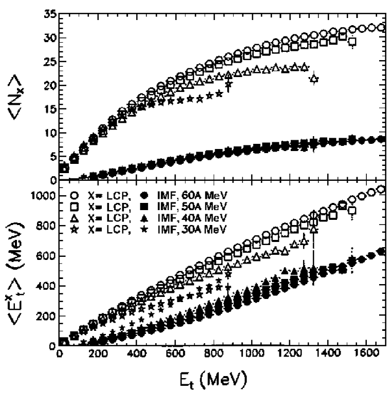
Figure 5: Top panel : average number of IMFs (solid symbols) and LCPs (open symbols) as a function of the total transverse energy $E_{t}$. Bottom panel : corresponding average transverse energies as a function of $E_{t}$. The different symbols correspond to different bombarding energies indicated in the bottom panel [143]. See text.

The fragmentation events observed in the reaction ${}^{129}Xe+^{197}Au$ at 30, 40, 50 and $60\,MeV\!\cdot\!A$ projectile energy have been analysed in some detail [143]. The average transverse energy $(E_{t}=\sum_{i}E_{i}\sin^{2}\theta_{i}\,$, where $E_{i}\sin^{2}\theta_{i}$ is the projection of the energy associated with species $i$ in the direction perpendicular to the incident beam) measures the energy transferred from the relative motion of the ions to the excitation energy of the system. The analysis shows that the average number of light charged particles $<N_{LCP}>$ and the average number of IMFs and their corresponding transverse energies increase monotonously with increasing $E_{t}$ as shown in Fig. 5. This contradicts the results of [144] where the transverse LCP energy saturates. This saturation can in fact be understood as being due to instrumental problems. The features observed in Fig. 5 can be interpreted and understood in the framework of a statistical decay mechanism [134]. The results can also be reproduced in the framework of phase space models like SMM [110].

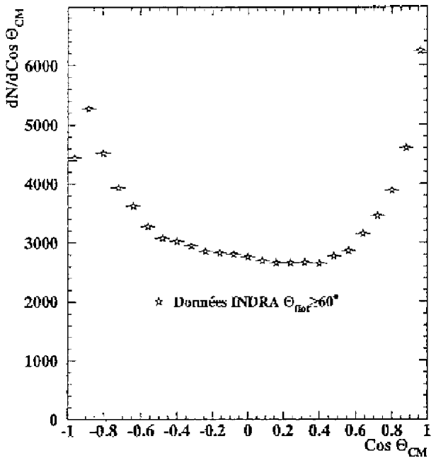
Figure 6: Angular distribution of light particles $(Z=1,2)$ in the flow angle $\theta\geq 60^{\circ}$ corresponding to events generated by a unique source in the reaction $Xe+Sn$ at $50\,MeV\!\cdot\!A$ [147].

Further analysis of the reaction ${}^{129}Xe+Sn$ have been presented and discussed in the recent past [145, 146, 147]. In ref. [146] correlation techniques were used in order to determine the multiplicities of $H$ and $He$ isotopes emitted by the excited fragments produced at the disassembly stage of an equilibrated hot source. The determination of LCP multiplicities and kinetic energies led to the fragment excitation energies. These energies per particle are the same for all IMFs, which is interpreted as a sign for the fact that thermodynamic equilibrium is established at the stage where the source decays. A very detailed analysis of the same reaction was presented and discussed in ref. [147]. It is shown there that the experimental fragmentation data can be interpreted in terms of unique source whose existence could be ascertained by means of kinematical arguments related to global observables like the collective flow angle. For events which are selected under specific criteria the angular distributions of light particles and intermediate mass fragments show the characteristic behaviour of statistical evaporation, i.e. approximate symmetry with respect to $90^{\circ}$, see Fig. 6, and excitation functions decrease exponentially as a function of energy. The experimental results were further confronted with simulations by means of the SMM model in its microcanonical version. This confrontation confirmed that the assumption of thermodynamic equilibrium is compatible with information extracted from experimental data. The analysis relies on the so called backtracing method developed in ref. [110] which solves the inverse problem by tracing back the issue of the process to the characteristics of its origin, i.e. the characteristics of an excited equilibrated source. This method has also been applied to experiments performed by the ALADIN collaboration at the GSI for reactions of ${}^{197}Au$ on $C,\ Al,\ Cu$ and $Pb$ targets at $600\,MeV\!\cdot\!A$ energy [148, 149, 150].

There exist some indications for equilibration from purely experimental origin [151], corresponding to so called spectator reactions, i.e. more or less peripheral heavy ion collisions, in particular ${}^{197}Au$ on ${}^{197}Au$ at high bombarding energies, 0.6 and $1\,GeV\!\cdot\!A$. In this type of reactions it is assumed that part of the nucleons, the spectators, form a highly excited system which experiences only disordered motion and from which any coherent collective motion is practically absent. Several arguments lead to the conclusion that these systems could be in thermodynamic equilibrium. Recently the relative velocity correlation between LCPs and fragments has been used in order to reconstruct the size and excitation energies of the so called primary fragments which are produced at the early stage of the collision of $Xe$ on $Sn$ at 32 and $50MeV\!\cdot\!A$ [152]. The constancy of the excitation energy imparted to the system with increasing bombarding energy suggests that thermodynamic equilibrium may be reached at freeze-out.

The fragment distributions are invariant with respect to the formation process, i.e. the entrance channel of the reaction. As we shall see in section 5, there has been an attempt to fix a temperature to the spectator system by means of the measurement of the isotope ratios of light nuclei $(He,Li)$ which are generated through fragmentation [153]. These ratios are invariant with respect to the bombarding energy. The result is however, at first sight, not compatible with other observables from which it is in principle possible to extract a temperature. This is so, in particular, for the slopes of the energy distributions of fragments which, if they are interpreted as Maxwellian distributions, lead to much higher temperatures. Several arguments which try to explain this fact have been proposed [151], among them the role played by the Fermi motion [154] of nucleons related to a fast fragmentation process.

The equilibration problem has also been raised by the FOPI collaboration in the study of reactions involving more central heavy ion collisions [89]. In this type of events, one observes a collective flow of particles. This fact complicates the experimental analysis and does not allow for a clear-cut conclusion about equilibration. Indeed, different models, both time-independent and time-dependent seem to be able to reproduce the data [155]. Recently isospin arguments have been used in order to test equilibration [156]. They indicate that equilibration is not reached as far as isospin degrees of freedom are concerned.

4 Percolation models and fragment size distributions

The detection and identification of the charge and the mass of fragments generated through violent collisions is of fundamental importance in the study of excited nuclei. Many detectors like ALADIN, FOPI, INDRA, the EOS setup, the MINIBALL, LASSA, CHIMERA are able to detect and identify particles and fragments event by event and to determine their asymptotic kinematical properties which constitute the information which can be experimentally collected.

As already seen above, the information contained in the outcome of processes like fragmentation are of extreme complexity and the formation mechanism largely unknown, certainly different under different physical conditions such as the energy range and the impact parameter. On the other hand, the use of the concepts of statistical mechanisms has shown that paradoxically the most complex systems can be described in terms of minimum information theories which bypass the detailed knowledge of the underlying microscopic systems. Here it may be tempting to follow this philosophy and to try to describe the outcome of nuclear fragmentation processes within the simplest possible physical framework. This has been done starting in the early 80’s by means of minimum information approaches like percolation models. These models ground on purely topological and statistical concepts, they avoid the explicit introduction of Hamiltonians. If they work, they raise of course the question why and how this is the case.

In percolation theories, space contains empty regions and parts which are occupied by individual objects which can be considered as bound to form larger entities defined by means of different criteria. The essential concepts are connectivity, localization and percolation which characterizes the properties of clusters (animals, fragments). Percolation itself is established when, in an infinite space, at least one cluster of infinite size is present.

Percolation models have been used in many fields which deal with geometry, disorder, statistics and physics such as aggregation, localization, diffusion, conductivity …Before going over to its application in the field of nuclear fragmentation it may be worthwhile to recall general concepts, definitions and properties which appear in the framework of this type of descriptions.

4.1 Random-cluster models : general concepts and properties

The first percolation model was introduced by Broadbent and Hammersley [157] in order to describe the spread of matter through a medium such as a liquid through a porous medium. It was then soon recognized that this type of model is acquainted to already known models like the Ising model [158] and other statistical spin models like those developed by Ashkin and Teller [159] and Potts [160].

All these descriptions can be studied in a general framework called random-cluster model. This has been worked out by Fortuin and Kasteleyn [161, 162]. In the first paper [161] the authors showed the close connection between the connectivity problem of different systems with uncorrelated bonds between sites which are occupied by single objects (particles) and the well known Ising model. Since Ising systems exhibit phase transitions in $2d$ and $3d$ spaces it is not surprising that the random-cluster model shows itself a phase transition in the infinite space limit. In later developments [162] the authors studied the general topological properties of the aforementioned models by means of graph theory, in particular those of the random-cluster model. They showed why the models quoted in refs. [158, 159, 160] as well as linear resistance networks and percolation models can be studied in a unique framework by means of graphs defined in terms of vertices (sites), edges (bonds), connections between edges and vertices, and probabilities $p$ for edges to exist or not. In practice they introduced a generalized partition function (cluster generation function) and “free energy” which enables to work out physical observables like thermodynamic quantities in the case of the Ising, Ashkin-Teller and Potts models and correlation functions.

Further analytical developments on percolation models were pursued by Kunz and Souillard [163, 164] related to previous work by E.H. Lieb. In the case where sites do not interact, i.e. are not correlated, they introduced the free energy

$$f_{p}(h)=\sum_{n}P_{n}\frac{e^{-hn}}{n}=\sum_{C}e^{-h|C|}\cdot\frac{p^{|C|}q^{\partial|C|}}{|C|}$$

where $p$ is the bond probability, $q=1-p$, $P_{n}$ the probability that a given site belongs to a cluster with exactly $n$ sites, $C$ are all finite clusters containing the origin of space $0$, $|C|$ is the size of the clusters and $\partial|C|$ the size of the boundary of clusters, i.e. their perimeters (surfaces). The study of the properties of $f_{p}(h)$ shows that this function is analytic for $h=0$ and $p<p_{c}$, and develops a singularity for $p\geq p_{c}$ if the system is infinite, indicating a phase transition of second order at $p=p_{c}$. For $p\geq p_{c}$ the system percolates in the sense defined above, i.e. at least one cluster of infinite size appears.

4.2 Percolation models : definitions and general properties

Before discussing the applications of percolation concepts to nuclear fragmentation we present here some essential properties of percolation models we shall need in the sequel.

Percolation models consist of a discrete number of sites which cover a finite or infinite part of a $d$-dimensional space [165, 166, 167]. Site percolation corresponds to the case where each site is either occupied by one “particle” or is empty. Bond percolation corresponds to the case where each site is occupied, neighbouring sites being bound or not to each other. The number of neighbouring sites is fixed by the connectivity which depends on the geometric structure of space occupation (f.i. a triangular lattice for $d=2$, a cubic lattice for $d=3$, …). The combination of site occupation and bond formation leads to hybrid site-bond models.

Except for the results presented in section 4.1 above [161, 162, 163, 164], very little is known analytically about these models. Most information has been gained by means of numerical simulations.

In the case of site percolation, one fixes a probability $p\in[0,1]$. For each site, one draws a random number $\eta$ taken from a uniform distribution in the interval $[0,1]$. If $\eta\leq p$ the site is said to be occupied, if $\eta>p$ it is empty. Hopping over all sites, one generates an ensemble of occupied and empty sites. If the number $N$ of sites gets very large, one finds $Np$ occupied and $N(1-p)$ empty sites. If neighbouring sites are occupied they belong to the same cluster. Space is finally covered with clusters and empty space.

A similar procedure works in the case of bond percolation. For a fixed bond probability $p$ consider a pair of neighbouring sites and draw a random number $\eta\in[0,1]$. If $\eta\leq p$ the sites are linked by a bond, if $\eta>p$ they are not. Testing this way all possible bonds between neighbouring sites generates linked clusters of bound sites, each cluster being made up of an ensemble of connected particles. The determination of the whole cluster network will be called event or realization. In each realization there are clusters of different sizes. They appear with a given multiplicity which depends of course on $p$. Averaging over many realizations leads to a characteristic cluster size distribution in the infinite system.

Clusters with a fixed size can have different shapes for $d\geq 2$. The average number of clusters of size $r$ per lattice site taken over a set of realizations is given by

$$n_{r}=\sum_{s}g_{rs}p^{r}(1-p)^{s}$$

where $g_{rs}$ is the number of clusters with size $r$ and perimeter $s$, the perimeter being the number of empty (non connected) sites which surround the cluster. Generally $g_{rs}$ is not analytically accessible. We shall come back to this point below.

Individual clusters of size $s$ can also be characterized by a “gyration” radius $R_{D}$, defined by

$$R_{D}^{2} = \sum_{i=1}^{s}\frac{|\vec{r}_{i}-\vec{r}_{0}|^{2}}{s}$$

$$\textrm{where}\quad\vec{r}_{0} = \sum_{i=1}^{s}\frac{\vec{r}_{i}}{s}$$

is the centre of mass of the cluster.

Then the average squared distance between two cluster sites is

$$2R_{s}^{2}=\sum_{i\neq j}\frac{|\vec{r}_{i}-\vec{r}_{j}|^{2}}{s^{2}}$$

If $g(r)$ is the probability that a site which is a distance $r$ apart from an occupied site belongs to the same cluster, one can define a correlation length $\xi$ such that [167]

$$\xi^{2}=\frac{\sum_{r}r^{2}g(r)}{\sum_{r}g(r)}$$ (4)

$2R_{s}^{2}$ is the average distance between two sites of a cluster and $sn_{s}$ the probability that a site belongs to a cluster of size $s$. Since such a site is connected to $s$ other sites the correlation distance $\xi$ can be rewritten as

$$\xi^{2}=\frac{2\sum_{s}R_{s}^{2}s^{2}n_{s}}{\sum_{s}s^{2}n_{s}}$$ (5)

As it has been mentioned above [161, 162, 163, 164] there appears a percolation (second order) phase transition for $d\geq 2$ and some value $p=p_{c}<1$. For $p>p_{c}$ one or several infinite clusters are present. The system is said to percolate. The value of $p_{c}$ depends on the dimensionality of the system, the type of percolation (site or bond) and its connectivity (the number of maximum occupied sites in the next neighbourhood of a site or possible bonds of a site to the nearest neighbours) [167].

The central observable in percolation physics is of course the cluster size distribution. In practice, nothing is known analytically about it, except for conjectures which agree very precisely with numerical simulations. For $p<p_{c}$ and clusters of large size $(s\to\infty)\ \ln n_{s}\propto-s$, i.e. one observes an exponential tail when space occupation (site percolation) or the number of bonds ( bond percolation) is sparse. For $p>p_{c}$ and $s\to\infty\ \ln n_{s}\propto-s^{1-1/d}$. As one can see the space dimension enters in the case where space occupation or the number of bonds is large. This is not the case in the non percolative regime. Finally for $p\simeq p_{c}$ and large clusters it has been conjectured [167] that

$$n_{s}(p)\simeq s^{-\tau}f\big{(}(p-p_{c})s^{\sigma}\big{)}$$ (6)

which is true for all percolation models, $\tau$ and $\sigma$ being universal exponents and $f$ a model dependent function. For $p=p_{c},\ f(0)=1$, leading to a power law behaviour which intriguinly reminds Fisher’s expression (1). As stated above, these relations are very accurately verified by numerical tests.

4.3 Moments of the cluster size distribution and critical exponents

For infinite systems it is possible to work out the expression of the cluster size distribution $n_{s}(p)$ in the vicinity of the critical point $p=p_{c}$.

By definition the $k$th moment is

$$m_{k}(p)=\sum_{s}s^{k}\cdot n_{s}(p)$$

Going over to the continuum limit

$$m_{k}(p)=\int_{0}^{\infty}\textrm{d}s\,s^{k}n_{s}(p)$$

and introducing the analytical expression (6) with

$$f\big{(}(p-p_{c})s^{\sigma}\big{)}=\exp(-|p-p_{c}|^{1/\sigma}s)$$

for $p$ in the vicinity of $p\sim p_{c}$ leads to

$$m_{k}(p) \sim |p-p_{c}|^{\mu_{k}}$$ (7)

$$\textrm{where}\quad\mu_{k} = \frac{\tau-k-1}{\sigma}$$ (8)

For $k>\tau-1$ one sees that the moments diverge at $p=p_{c}$, a sign for the existence of a phase transition. Hence, if $\tau<3$ which is the case for $d=2,3$

$$m_{2}(p) \sim |p-p_{c}|^{-\gamma}$$

$$\textrm{with}\quad\gamma = (3-\tau)/\sigma$$ (9)

For $d=3$ in a cubic lattice $\gamma=1.74$.

Critical exponents characterize other quantities of interest. If in the infinite system $P(p)$ is the probability that a given site belongs to the infinite cluster for $p>p_{c}$, then probability conservation implies

$$P(p)+(1-p)+\sum_{s}sn_{s}(p)=1$$

The second term corresponds to the probability that the site is empty and the third that it belongs to a finite cluster of size $s$.

$$\textrm{At}\quad p=p_{c}\quad P(p_{c})= 0$$

and $$\sum_{s}sn_{s}(p_{c})= p_{c}$$

Hence in the vicinity of $p_{c}$, $P$ can be written [167]

$$P=\sum_{s}[n_{s}(p_{c})-n_{s}(p)]s+\mathcal{O}(p-p_{c})$$ (10)

If one introduces the parametrization $n_{s}(p)\propto s^{-\tau}\exp(-cs)$ with $c=0$ at $p=p_{c}$ and goes over to the continuum limit with (10) it comes

$$P \propto (p-p_{c})^{\beta}$$

$$\textrm{where}\quad\beta = (\tau-2)/\sigma$$ (11)

which consistently tends to zero when $\tau>2$ at $p=p_{c}$.

Since percolation systems show a continuous transition at $p=p_{c}$ one expects that the correlation length $\xi$ defined in (4) shows a singular behaviour at the threshold where an infinitely large cluster merges. This is indeed the case

$$\xi\propto|p-p_{c}|^{-\nu}$$ (12)

and the positive exponent $\nu$ can be determined numerically.

Percolation clusters are generally fractal objects. The radius of gyration $R_{D}$ is related to the volume $s$ through

$$s\propto R_{D}^{d_{f}}$$

where $d_{f}$ is an effective, not necessarily integer space dimension. From the expression (5) it follows that $\xi^{2}$ behaves like $s^{2+2/d_{f}}$. The same type of derivation as the one used for the moments $m_{k}(p)$ leads to a power law expression of $\xi^{2}$ whose numerator diverges with an exponent $(3-\tau+2/d_{f})/\sigma$. Hence $\xi^{2}$ itself diverges like $2/d_{f}\sigma$ and an identification with (12) leads to

$$\sigma\nu=1/d_{f}$$ (13)

At $p=p_{c}\quad R_{s}\propto s^{1/d_{f}}$, hence the size of the largest cluster increases like $L\propto s^{1/d_{f}}$. If $P$ is the strength of the infinite cluster as defined above, $PL^{d}$ is the volume occupied by the largest cluster. If the linear extension of this cluster is of the order of the correlation length $\xi$

$$PL^{d} \propto L^{d_{f}}$$

$$L \propto \xi\propto|p-p_{c}|^{-\nu}$$

Recalling the behaviour of $P$ in the neighbourhood of $p_{c}$ one gets

$$d_{f}=d-\beta/\nu$$ (14)

In summary, general considerations lead to six critical exponents $\tau,\sigma,\beta,\nu,d_{f},\textrm{and }\gamma$ which are linked by four relations (9), (11), (13) and (14).

Up to now we considered essentially the properties of infinite systems and concentrated on their behaviour in the vicinity of the percolation threshold which allows to determine critical exponents. These exponents are very useful quantities since they fix the universality class to which a critical system belongs. If excited nuclei are the finite counterparts of critical nuclear matter, the singular behaviour of observables at the phase transition is quantitatively characterized by critical exponents. We shall try to see and to understand below if, how and why percolation concepts could be related to nuclear fragmentation. But nuclei are finite systems. Before we present and discuss the models which have been proposed, we present a study of the effects generated by the finiteness of percolation systems.

4.4 Finite size constraints on random-cluster systems

Percolation deals with the critical behaviour of systems in the limit of infinitely extended space. Microscopic and mesoscopic systems like nuclei, atoms, molecules, aggregates are finite. As far as percolation concepts can be applied to their description and directly compared to experiment as we shall do below, it is necessary to get some insight into the behaviour of percolation models in finite space. Finite size effects enter because of the presence of a surface which induces constraints on the system, especially when the space occupation is large. We concentrate here on site percolation.

The aim of the study concerns the determination of the fragment size distribution of a system with $V$ sites, with an occupation number equal to 0 or 1 for each site. The number of occupied sites $A$ is fixed, the density is $\rho=A/V$. Following percolation concepts one qualitatively expects a set of small clusters when $\rho$ is small, hence a cluster size distribution which decays monotonously as a function of the cluster size and for large values of $\rho$ one or several large clusters together with small clusters showing a kind of $U$-shape. For intermediate values of $\rho$ small and intermediate size clusters may coexist. These shapes are in fact observed in the experiment. The crucial point concerns the behaviour of the distribution for these intermediate values of $\rho$.

The behaviour of finite percolation systems has been investigated in [168]. One considers a finite volume $V$ in a $d$-dimensional space. Space occupation by $A$ particles is defined by $O=(i_{1},\ldots,i_{A})$ where $i_{1},\ldots,i_{A}$ label $A$ occupied sites. There are $\binom{V}{A}\equiv V!/A!(V-A)!$ possible arrangements. To each occupation can be attributed a canonical weight, $\exp[-\beta H(O)]$ where $H$ is the Hamiltonian of the system and $\beta$ can be interpreted as an inverse temperature. Define

$$H(O) = \frac{1}{2}\sum_{i\neq j}H_{ij}$$

$$\textrm{with}\quad H_{ij} = H_{ji}$$

A simple choice would be

$$H_{ij}=-eL_{ij}$$

where $e$ is a positive constant and $L_{ij}\ (i\neq j=1,\ldots,V)$ taking values 0 and 1 defines a link structure which decides whether two sites are connected or not.

The link structure introduces the concept of clusters as sets $c$ of connected occupied sites $c=(i_{1},\ldots,i_{a})$, with size $a(c)$ and a surface (called perimeter in section 4.1) made of those unoccupied sites which are the nearest neighbours of occupied ones.

Given a cluster of size $a$ and surface $s$, we call $f(c)=V-a-s$ the free complement of $c$ which is such that

$$c\cup s\cup f=V$$

The central observable is the average multiplicity of clusters of a given size in the canonical ensemble, allowing for all possible occupations with fixed $a$, weighted by the Boltzmann factor $\exp(-\beta H)$.

The average of an observable $\Omega$ is defined by

$$<\Omega>=\frac{1}{\mathcal{Z}}\sum_{O\subseteq V}\Omega(O)\exp[-\beta H(O)]\,\delta\big{(}a(O)-A\big{)}$$

where obviously

$$\mathcal{Z}=\mathcal{Z}(V,A,\beta)=\sum_{O\subseteq V}\exp[-\beta H(O)]\,\delta\big{(}a(O)-A\big{)}$$

is the canonical partition function. In particular, the energy $U$ and the entropy $S$ read

$$U = <H>$$ (15)

$$S = \ln\mathcal{Z}+\beta U$$

Notice that, as generally admitted in random-cluster models, there exists no cluster-cluster interaction. This is due to the fact that the interaction is restricted to nearest neighbour occupied sites.

The probability to find a cluster $c$ of size $a$ in a configuration is given by

$$P(c)=e^{-\beta H(c)}\mathcal{Z}(f,A-a,\beta)/\mathcal{Z}(V,A,\beta)$$

Then

$$<\Omega>=\sum_{c}P(c)\Omega(c)$$

for any observable $\Omega$.

In particular, the multiplicity of clusters of size $a$ is given by

$$m(a)=\sum_{c}P(c)\delta\big{(}a-a(s)\big{)}$$

The essential constraint on $m(a)$ is fixed by the fixed number of particles

$$\sum_{a=1}^{A}a\,m(a)=A$$ (16)

Monte Carlo simulations [168] reproduce the expected cluster size distributions which were predicted above, in particular the $U$-shape at large density. This is true both in the case when the coupling constant $e$ is zero or finite except that the transition from the falling distribution for small $\rho$ to the $U$-shape is located at different values of $\rho$ for different values of $e$. Hence in order to study the consequences of the constraint imposed by (16) one may restrict this study to the case $e=0$ which allows for the use of simple analytical arguments. Then

$$\mathcal{Z}(V,A) = \binom{V}{A}$$

$$m(a) = \sum_{s}g(a,s)\binom{V-a-s}{A-a}\Big{/}\binom{V}{A}$$

where s is the surface defined above and $g(a,s)$ the number of clusters of size $a$ and surface $s$.

In the case where the system is dilute $(\rho=A/V\ll 1)$

$$m(a)=\sum_{s}g(a,s)\rho^{a}(1-\rho)^{s}$$ (17)

The degeneracy $g$ is a complicated function of the link structure $L$. There exists some knowledge about it [165, 166, 169]. In fact $g(a,s)$ differs from zero only in a narrow range of surfaces.

It is convenient to introduce

$$g(a,s)=\gamma(a)P_{a}(s)$$

where $P_{a}(s)$ is the distribution of surface sizes for fixed $a$. The surface $s$ varies between a minimum and a maximum limit for fixed $a$. The minimum is given for the more compact forms

$$s_{min}(a) \propto a^{1-1/d}\quad\quad\quad\quad\textrm{for}\quad a<\frac{V}{2}$$

$$\propto (V-a)^{1-1/d}\quad\textrm{for}\quad a>\frac{V}{2}$$

The maximum corresponds to chain-like clusters, hence

$$s_{max}(a)\propto 2+2(d-1)a$$ (18)

in a $d$-dimensional hypercubic lattice. Of course $s\leq V-a$.

The overall behaviour of the surface as a function of the cluster size is shown in Fig. 7. If one defines an average surface

$$\sigma(a)=\sum_{s}sP_{a}(s)$$

then for the small mass sector one may parametrize $\sigma(a)$ in the following form

$$\sigma(a)=\lambda a+\sigma_{0}\quad a\ll A_{0}\,,\quad\lambda\leq 2d-2$$

and for the large mass sector

$$\sigma(a)=K(V-a)\quad a\gg A_{0}\,,\quad K\leq 1$$ (19)

where $A_{0}$ is the solution of $s_{max}(A_{0})=V-A_{0}$, see (18). Hence

$$2(d-1)A_{0}+A_{0}=V-2$$

and

$$A_{0}=(V-2)/(2d-1)$$

Consider first the small mass sector. Since the distribution $P_{a}(s)$ is not known, one might investigate different types of distribution. Analytic results can be obtained for a Poisson or a sharp distribution. In the simplest case

$$P_{a}(s)=\delta\big{(}\sigma(a)-s\big{)}$$ (20)

The distribution may indeed be rather sharp when $a$ does not get too large, see Fig. 7. Then, using (20) one obtains

$$G(a)=V\sigma(1)[\sigma(a)+a-2]!/[a!\,\sigma(a)!]$$

For $a,\sigma\gg 1$

$$G(a) \propto a^{-2.5}\exp(\alpha_{c}a)$$

$$\textrm{with}\quad\alpha_{c} = \ln[(\lambda+1)^{\lambda+1}/\lambda^{\lambda}]$$

A similar expression for $G(a)$ is obtained if $P_{a}(s)$ is a Poisson distribution. As a consequence

$$m(a) \propto a^{-2.5}\exp\{(\alpha_{c}-\alpha)a\}$$

$$\textrm{with}\quad\alpha = \ln[1/\rho(1-\lambda)^{\lambda}]$$

$\alpha$ is minimum for $\alpha=\alpha_{c}$ at

$$\rho_{c}=1/(1+\lambda)$$

Then $m(a)\propto a^{-2.5}$ for $\rho=\rho_{c}$. One again finds the manifestation of a power law behaviour, which is realized in the case of finite systems.

If $V$ is large $\sigma(a)$ lies close to $2(d-1)a+2$, hence $\lambda=2d-2$ for cubic lattices. Then

$$\rho_{c}=1/(2d-1)=A_{0}/V$$

In fact $\rho_{c}$ is determined by the crossing of the two topological limits fixed by the small and large cluster sector. Hence in finite systems the onset of a “critical” regime is correlated with a topological constraint which, in a finite but large volume, corresponds to cluster surfaces with a maximum in the vicinity of $\rho_{c}V=V/(2d-1)$.

In the case of large $\rho$ it is sensible to parametrize the surface following (19) above. Then

$$m(a)\propto q^{A-a}/(A-a)!$$

with

$$q=\{(V-A)/\big{(}A+K(V-A)\big{)}\}^{1-K}A(1-K)K^{-K}$$

This distribution is monotonically rising with $a$ if $K<K_{cr}\sim A/(A+1)$ and reaches a maximum at $a=A$. In all other cases it peaks at $q\simeq A-a$. For $s_{min}(a)>V-a,\ m(a)$ is of course zero.

In summary, simple considerations lead to a different behaviour of cluster size distributions in different density sectors of finite systems. This behaviour is essentially governed by the mass conservation constraint (16) imposed by the finite volume in which the system is located. For small densities the size distribution decreases essentially as an exponential. There exists a density $\rho_{c}$ for which the distribution is a power law or close to it, with a fixed index irrespective of the dimensionality of space. For $\rho>\rho_{c}$ one observes both a decreasing light cluster sector and a large size sector building up.

The present results are general. As we shall show below they are in qualitative agreement with explicit simulation results and experimentally observed cluster size distributions.

4.5 Models related to percolation and first confrontations with the experiment

The first applications of percolation concepts to the description of nuclear fragmentation were proposed by Bauer and collaborators [170, 171], Campi and Desbois [172].

The starting point of Bauer et al. was the observation of the power law distribution of intermediate mass fragments [18, 21, 22] obtained by means of fragmentation processes

$$A_{p}+A_{t}\to A_{f}+X$$

where $A_{p},A_{t},A_{f}$ are the mass of the projectile, target and a specific fragment and $X$ the rest of the reaction outcome.

In the absence of any precise information about the reaction mechanism the authors [170, 171] suggested a minimal-information description, following the same spirit as the one which prevailed in ref. [173]. They introduced a nucleus lattice model (NLM) in which a set of particles occupy lattice sites in a finite space. The presence of bond clusters is tested by means of a bond percolation algorithm as described above applied to a $3d$ cubic lattice model in a finite volume. The so called standard percolation theory (SPT) deals with infinite systems. The physical framework here is an $A+1$ particle system obtained by means of energetic collisions of a proton on a nucleus. The penetration of the proton generates a cylindrical tube of radius $r$ with very excited matter (fireball), in an initial spherical nucleus at an impact parameter $b$. The nucleons of the fireball are kicked out, the remaining nucleons are sitting on lattice sites and experience a strong disturbance which reflects in the definition of a bond breaking probability $p$ characterizing the link between the remaining spectator nucleons. In this description the exact number of particles is not fixed and there is no information about the energy imparted to the system. The bond breaking probability $p$ is supposed to be the larger, the larger the kinetic energy of the incoming projectile proton. A Monte Carlo percolation algorithm applied to the system for different values of $p\in[0,1]$ leads to different shapes of the fragment (cluster) size distribution, ranging from an $U$-shape for small $p$ to a typical exponential fall-off with no heavy fragments available for large $p$, as predicted in ref. [168]. For some $p\simeq p_{c}\simeq 0.74$ the width of the mass distribution gets maximum and the mean yield shows a power law behaviour for light and intermediate mass fragments, with an exponent $\tau\simeq 2.21$. This value is somewhat lower than the one corresponding to the infinite system.

This bond-breaking model was confronted with experimental results concerning the reactions $p+Ag$, $p+Ta$ and $p+Au$, for proton energies of several $GeVs$. If the bond probability $p$ is parametrized in terms of the impact parameter as

$$p(b)=p_{0}/[1+\exp\big{(}(b-R)/d\big{)}]$$

where $R$ is the radius of the system, $b$ the impact parameter an $d$ a diffusion coefficient, one finds a very good agreement between calculated and experimental fragment size distributions, see Fig. 8, by sampling over the whole range of impact parameters, $b$ = 0 to $R$. In order to get a closer link between percolation calculations it is sensible to replace $p$ which is not an observable by the average over realizations of the fragment multiplicities $m$ obtained for a fixed value of $p$. This allows to relate $\tau$ extracted from a power law fit of the fragment size distribution to an average multiplicity at the “critical” point, $<m>_{c}$.

The strikingly good agreement between the application of simple percolation concepts and the outcome of inclusive observables extracted from complex collision processes raises several questions. The model does not care about mass and energy conservation, possible geometrical deformation effects when the fragmenting system is generated through heavy ion collisions. The bond probability is necessarily related to the microscopic dynamics. It may be asked why this unique parameter parametrizes so perfectly the underlying interaction between the nucleons in the excited nuclear medium. We shall come back to this point in section 5.

In a similar spirit, Campi and Desbois [172] developed a continuum site percolation approach.$\ A_{T}$ particles occupy an ensemble of points $\{\vec{r}_{i},\vec{p}_{i},i=1,\ldots,A_{T}\}$ in phase space chosen in a classical one-body Wigner distribution $f_{W}(\vec{r},\vec{p})$ determined by a one-body Hamiltonian with a Saxon-Woods potential. The collision process leaves $pA_{T}$ nucleons of the original nucleus, $(1-p)A_{T}$ nuleons are kicked off the original nucleus, $p\in[0,1]$ depends on the characteristics of the reaction like impact parameter, energy, target size …Clusters are generated by means of phase space prescriptions which decide whether particles belong to fragments or not. A given number of particles forms a bound cluster if

$$d_{ij}=|\vec{r}_{i}-\vec{r}_{j}|\cdot|\vec{p}_{i}-\vec{p}_{j}|\leq 2.5\hbar$$

for every pair of nearest neighbours belonging to the supposed cluster, where the maximum action on the r.h.s. of (4.5) corresponds to the value obtained for the deuteron. This condition is supplemented by a compactness constraint which imposes that the mean square radius $R_{A}$ and mean square momentum $p_{A}$ verifies

$$R_{A} \leq (1+\epsilon)r_{0}A^{1/3}$$ (21)

$$p_{A} \leq (1+\epsilon)\Big{(}\frac{3}{5}\Big{)}^{1/2}p_{F}^{1/2}$$

where $p_{F}$ is the Fermi momentum and $\epsilon\simeq 0.12$. If the constraints (21) are not fulfilled the longest link $d_{ij}$ is cut and the determination of clusters starts again. The first condition takes care of the balance between volume and surface energy of the cluster, the second eliminates nucleons with too large momenta. The model is constructed with percolation concepts which do however not correspond to the standard ones, essentially because the generation algorithm is not fixed by a single and simple bond probability parameter. The cluster multiplicity obtained in this way can be fitted by means of parametric analytical expressions [172]. The generated clusters are excited objects whose excitation energy $E^{*}$ can be estimated. Particle emission from fragments and their fission are taken into account.

In order to enable the confrontation of the model with experiment, the quantity $p$ which fixes the number of remaining nucleons after the collisions is related to the number of nucleon-nucleon collisions which are experienced in the system for a fixed impact parameter $b$ and nucleon mean free path $\lambda$ which varies with the energy. This leads to a distribution for $p,\ \rho(p)$, for $p$ larger than a value $p_{min}$ corresponding to $b=0$. Depending on the physical conditions, $p$ can reach or not the percolation threshold. One can then calculate explicitly inclusive mass yields for fragments of size $A_{F}$

$$\sigma(A_{F})=\int_{p_{min}}^{1}\mathrm{d}p\,\rho(p)\,m(p,A_{F})$$

where $m(p,A_{F})$ is the multiplicity of fragments of size $A_{F}$, for a fixed value of $p$, and the total reaction cross section

$$\sigma_{R}=\int_{p_{min}}^{1}\mathrm{d}p\,\rho(p)$$

The model reproduces very well the fragment size yields $\sigma(A_{F})$ for low and high energy data corresponding to ${}^{20}Ne+^{181}Ta$ at $400\,MeV\!\cdot\!A$, $p+^{181}Ta$ at $5.7\,GeV$ and $p+^{181}Ta$ at $340\,MeV$. In the lower energy data one observes the opening of the fission channel which is predominant along with particle evaporation at this energy. For high energy reactions, $p+Xe$ at $80-350\,GeV$, both the slope and absolute value of $\sigma(A_{F})$ are well reproduced. The trend of the apparent “critical” exponent $\sigma(A_{F})\propto A_{F}^{-\tau(E)}$ where $E$ is the bombarding energy shows a minimum $\tau\sim 2.4$ at $E=50\,GeV$. This is understood in the following way. When $E$ is small $p_{min}$ is large, $p_{c}$ cannot be reached, hence the system is essentially made up of one large cluster and a set of small particles. When $E$ increases $p_{min}$ decreases, $p_{c}$ can be reached and one gets a power law distribution over the whole range of fragments sizes, except for finite size effects. For large value of $E$ $p_{min}$ continues to decrease, more and more smaller fragments are generated and the apparent slope of the distribution increases again. At very high energy the nucleon mean free path $\lambda(E)$ becomes constant, hence $p_{min}$ and $\tau$ saturate.

4.6 Relevant observables and percolation analysis of experimental data

The first extensive confrontation between standard percolation theory and nuclear fragmentation was initiated by Campi [174]. The phenomenon was interpreted as a bond-breaking process between bound nucleons due to the energy supplied to the system under violent collision conditions. As discussed in section 4.3, the moments $m_{k}$ of the fragment size distribution get singular at $p=p_{c}$ for $k\geq 2$, so do the normalized moments $S_{k}=m_{k}/m_{1}$. Hence one expects that they show a maximum in the vicinity of $p\sim p_{c}$. Since $m_{k}\propto\exp(-\mu_{k})$ with $\mu_{k}=(\tau-1-k)/\sigma$ (see (7) and (8)) at $p_{c}$, there should exist a linear relation between $\ln S_{k}$ and $\ln S_{l}$ at $p_{c}$. For $k=2$ and $l=3$ the slope can be written as $\ln S_{3}=\lambda\ln S_{2}$ with $\lambda=1+1/\sigma\gamma$ and one can in principle read off the value of the power law exponent $\tau$.

The introduction of $m_{k}$ and $S_{k}$ allows for a direct comparison between the moments obtained from bond percolation models (here $3d$ cubic) and those obtained from the experiment, $m_{k}^{j}$, which can be determined from the fragment size distributions of a set of events labelled by the index $j$ by taking an average over all available events. Another interesting observable is given by [175]

$$\gamma_{2}=\frac{m_{2}\cdot m_{0}}{m_{1}^{2}}$$ (22)

which is related to the variance $\sigma$ of the fragment size distribution by

$$\gamma_{2}=1+\sigma^{2}\cdot m_{0}^{2}/m_{1}^{2}$$

and should also show a sizable enhancement at the “critical” threshold.

Finally the last observable proposed in ref. [174] concerns the behaviour of the largest cluster $A_{max}$ in the system. Indeed, in the infinite system, $A_{max}$ should get infinite at criticality, hence it is expected to get large when $S_{2}$ gets large. Hence the correlation between $A_{max}$ and $S_{2}$ is expected to contain information of interest.

Bond percolation calculations in a cubic lattice in a finite system were performed for different sizes and $S_{2},S_{3},\gamma_{2}$ and $A_{max}$ were calculated. The average quantities were confronted with the outcome of a few hundred events generated by the fragmentation of ${}^{197}Au$ nuclei in emulsions [176]. Typical fission events involving two large fragments were excluded. Results are shown in Fig. 9 which relates $S_{3}$ and $S_{2}$ for both experimental events and percolation simulations. “Critical” events correspond to large values of $S_{2}$ and $S_{3}$. Violent $(p=0)$ and smooth $(p=1)$ collision events correspond to small values of $S_{2}$ and $S_{3}$. One observes that there is a striking agreement between the two results. It should be noticed that in both cases one mixes events which correspond to different values of $p$ (as far as calculations are concerned) and multiplicities which are related to the degree of violence of the process (as far as the experiment is concerned). They both show the expected linear behaviour which can be related to the presence of “critical” events. It is also remarkable to notice that the slopes $\lambda\simeq 2.22$ are in both cases very close to the value $\lambda=2.25$ corresponding to bond percolation in the infinite system. The same type of agreement can be observed when dealing with $S_{5}$ vs. $S_{2}$ [174]. In Fig. 10 $\,\gamma_{2}$ is drawn as a function of the average multiplicity $m_{0}$. The similarity of simulation results and experiment is again remarkable. One observes an enhancement in the neighbourhood of $m_{0}\simeq 0.25$ which, when related to the bond probability $p$, corresponds to $p\sim p_{c}$ in $3d$ cubic systems. The fact that $\gamma_{2}>2$ for $m_{0}\simeq 0.25$ indicates a power law distribution. Finally Fig. 11 compares the behaviour of $A_{max}$ as a function of $S_{2}$ in both cases. “Critical” events are concentrated in the right corner of the figure. One observes again a strong agreement between calculations and experiment.

The possibility to extract values of $\lambda$ and $\tau$ and the fact that these are close to standard percolation results may induce the temptation to conclude about the universality class of the apparent critical phenomenon unravelled by the present studies. One must however be careful, because different types of transitions may lead to exponents which lie close to each other but correspond to different classes. The determination of exponents needs some care. We shall come back to the problem concerning the determination of critical exponents in section 5.

4.7 Extensive tests on peripheral collision data : analysis of ALADIN experiments

Many experimental efforts have been made over the last decade by the ALADIN collaboration of the GSI in order to collect a large amount of significant information about particle and fragment multiplicities generated in the fragmentation of the projectile by means of energetic peripheral heavy ion collisions. Such precise and complete information allowed for a careful comparison with theoretical approaches, in particular percolation and percolation-inspired models. The first measurements which were performed established correlations between the multiplicity of light particles $M_{lp}$, the charge $Z_{max}$ of the largest fragment in an event and the sum of the charges of the fragments with $Z\geq 2,\ Z_{bound}$ [148]. It was found that the correlation between the multiplicity of intermediate mass fragments (IMFs), i.e. fragments with $3\leq Z\leq 30$ and $Z_{bound}$ was independent of the target nucleus. This was interpreted as a sign for the equilibration of the projectile remnant (spectator particles) before decay. The first detailed investigation of the average multiplicity of IMFs, $<M_{IMF}>$, showed that with increasing energy transferred to the projectile in reactions of $Au$ on $C,Al$ and $Cu$ targets $<M_{IMF}>$ first increases to a maximum and then decays [149]. This could be interpreted in the following way. For small energies peripheral collisions lead essentially to one large projectile remnant and a few light particles. With increasing energy, the projectile breaks up into more and more IMFs. If the energy gets very large most fragments are very small, $(Z\leq 2)$ and hence $<M_{IMF}>$ decreases again. These results were then compared to theoretical investigations of $<M_{IMF}>$ vs. $Z_{bound}$ [150] by means of the statistical models of Copenhagen [123, 124, 125] and Berlin [122], and a sequential decay scenario [177]. It is seen that sequential evaporation cannot reproduce the data.

An extensive analysis concerning the reactions with $Au$ on $C,Al,Cu$ and $Pb$ at $600\,MeV\!\cdot\!A$ was performed in ref. [178]. The charge distribution was fitted by a power law and the exponent $\tau$ showed a minimum somewhat below 2 when represented as a function of $Z_{bound}$. The average largest fragment charge $<Z_{max}>$ increases with increasing $Z_{bound}$. Other correlation functions like $\gamma_{2}$ (see above) and

$$A_{3}=[(Z_{max}-<Z>)^{2}+(Z_{2}-<Z>)^{2}+(Z_{3}-<Z>)^{2}]^{1/2}/\sqrt{6}$$

$$\textrm{where}\quad<Z>=\frac{1}{3}(Z_{max}+Z_{2}+Z_{3})$$

and $Z_{2}$ and $Z_{3}$ are the second and third largest fragment charges were determined.

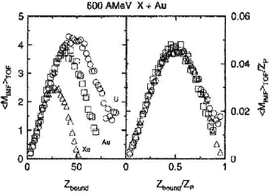
Figure 12: Left: measured mean multiplicities $<M_{IMF}>$ as a function of $Z_{bound}$ for ${}^{238}U$ on ${}^{197}Au$ (circles), ${}^{197}Au$ on ${}^{197}Au$ (squares) and ${}^{129}Xe$ on ${}^{197}Au$ (triangles) for $E=600\,MeV\!\cdot\!A$. Right: same quantities but rescaled by normalization with respect to the number of charges $Z_{p}$ of the projectile [179].

All results showed the striking feature that it is a simple-minded $3d$ site-bond percolation model with an occupation probability $p_{s}$ for the site and a fixed bond probability $p_{b}=0.45$ obtained through a fit to the $Z_{max}$ distribution which reproduces the best the available data. Masses in the percolation calculations were converted into charges by means of a semi-empirical mass formula [178]. The investigation of projectile fragmentation was finally extended to other projectiles like ${}^{129}Xe$ and ${}^{238}U$ with $Be,C,Al,Cu,In,Au$ and $U$ targets and energies ranging from 400 to $1000\,MeV\!\cdot\!A$ [179]. The striking feature about the results concerns the energy independence of $<M_{IMF}>$ as a function of $Z_{bound}$ and its scaling properties, i.e. all curves get superposed on each other if $Z_{bound}$ is rescaled to $Z_{bound}/Z_{p}$, where $Z_{p}$ is the charge of the projectile as it can be seen in Fig. 12. Statistical multifragmentation models reproduce qualitatively if not quantitatively the experimental results.

Recent ALADIN data concerning fragment size multiplicities for ${}^{197}Au$ on different target reactions at $600\,MeV\!\cdot\!A$ were analysed by means of a standard $3d$ cubic bond percolation model [180]. Depending on the value of the impact parameter, the number of spectator nucleons which remains in the projectile remnant is of course different. In order to decide about this number, a simulation by means of a BUU transport equation of the reaction process was performed. The spectator nucleons were arranged on a cubic lattice in a compact spherical arrangement and a bond percolation algorithm was introduced. Masses were converted into charges by means of the relation

$$Z=A/(1.98+0.0155A^{2/3})$$

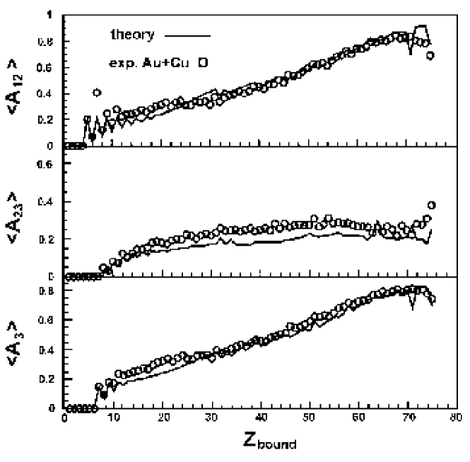
Figure 13: Average values of different observables defined in the text as a function of $Z_{bound}$ [180].

for $A\geq 4$. A filter was applied to the results of the calculations in order to allow for a direct confrontation between the model calculations and the experimental data. A whole set of observables was analysed in this way. Fig. 13 shows the average value of $A_{12}=(Z_{max}-Z_{2})/(Z_{max}+Z_{2}),\ A_{23}=(Z_{2}-Z_{3})/(Z_{2}+Z_{3})$ and $A_{3}$ defined above as a function of $Z_{bound}$. As one can see the agreement with the experiment is nearly perfect and this is also the case for all other observables.

A new analysis of the data [181] confirms this statement. The authors also use a standard $3d$ bond percolation algorithm. The number of nucleons $Z_{PS}$ which is taken into account [182] is parametrized in terms of $Z_{bound}$. Simulations are done for fixed $Z_{PS}$ and observables are determined for fixed $Z_{bound}$. The analysis is again parameter free. The calculated quantities are the fragment charge distributions, the average size and fluctuations of the largest fragment, and the largest fragment distribution. The confrontation also shows that there appears a “critical” regime, characterized by a power law charge distribution with $\tau\simeq 2.2$. In the neighbourhood of the “critical” point the distribution of fragments with charge $z$ can be parametrized as

$$n(z)=n_{c}(z)f(z/\overline{z})$$

where $\overline{z}=m_{3}/m_{2},\ m_{k}$ being the moment of order $k$ defined in section 4.3.

The authors consider two interpretations of these results. The first relies on the fact that a fragmenting nucleus is made of particles which interact essentially as nearest neighbours through a short range two-body potential. If the relative kinetic energy between pairs of neighbouring particles is larger than the potential energy they experience a bond is broken and hence independent fragments are generated if the excitation energy is large enough. The second interpretation requires the assumption of thermodynamic equilibrium. At different fixed densities it is the temperature $T$ of the system which fixes its fragment content. For a given density $\rho$ of the system, there exists a temperature $T(\rho)$ where the distribution looks like a power law. We shall come back to explicit classical microscopic model illustrations of both interpretations in section 5 below. It is clear that thermodynamic equilibrium is not a necessary prerequisite for an accurate description of the fragment content of energetic nuclear collisions.

4.8 Comparison with other fragmentation models

The intriguing and impressive success of classical percolation models in the description of finite nuclear fragmentation events and the existence of a continuous phase transition in infinite percolation systems triggered many attempts to compare and possibly relate different models with the percolation approach. Such attempts started with the Statistical Multifragmentation Model SMM [125]. The authors tried to establish a link between the percolation bond probability $p$ and the excitation energy available in the fragmented system described by SMM [124] at freeze-out. They fixed $p=V_{0}/(V_{0}+V_{f})$ where $V_{0}$ is the volume of the initial compact system and $V_{f}$ the volume at freeze-out. The investigations revealed that such a link is not clearly established and led to the conclusion that inclusive fragment size distributions may not contain enough information in order to distinguish the purely statistical features of the fragmentation process from those which concern physical information carried in phase space models.

A detailed comparison of the fragment content obtained in the framework of the MMMC model [79] with percolation was carried out in ref. [183] by means of an analysis of the relation between the charge of the heaviest fragment and the second moment of the charge distribution [174]. Close similarities between MMMC and percolation models were found, in particular the “critical” zone which was discussed in section 4.6. The main qualitative difference between the two approaches is the manifestation of the presence of fission events (two heavy fragments) which are absent in the percolation simulations. This was interpreted as being due to the presence of the long range Coulomb interaction which is not taken into account by the percolation model. Three-body correlations between the three heaviest fragments were also in agreement with the percolation predictions. So called cracking events with more than two large fragments emphasized the role and importance of the Coulomb interaction.

Moment correlations [173, 174] have been used in order to test different models and possibly discriminate between them [184]. The models which are introduced are an equal probability model for the generation of different partitions [186, 187], time-dependent sequential decay processes [94, 185] and a standard bond percolation model on a finite cubic lattice. All models agree qualitatively with percolation calculations but do not reach quantitative agreement. The peak corresponding to “criticality” in percolation is always present, but it is shifted in the multiplicity and its height is not reproduced. As expected, the agreement between percolation calculations and experiment is excellent.

A model analysis of data has also been performed by Kreutz et al. [178] with a statistical decay model [177], SMM and, as already discussed above, a site-bond percolation model. It appears again that all models lead to quantitatively different results. Sequential decay fails to reproduce charge correlation measurements, $<\gamma_{2}>$, charge distributions and IMF multiplicities come out more or less closely to experiment in SMM, although the average largest fragment charge is too small.

4.9 Final remarks

If one restricts the information concerning the fragmentation of highly excited nuclei to the description of the asymptotic fragment size distribution it appears clearly that parameter free standard percolation models are the only ones which are able to reproduce the experimental data quantitatively. It raises the up to now unanswered question why this is so. It shows that a minimum information model is sufficient in order to explain the a priori complex nuclear fragmentation process. The agreement is by essence independent of any detail concerning explicit two-body potentials. As it will be seen later, simple models governed by short range interactions are able to reproduce percolation results. The long range Coulomb interaction which induces fission-like fragmentation is out of reach. The fact that its absence does not affect the physics of the process may be understood if the excitation energy is large enough. The influence of the Coulomb interaction will be more extensively discussed in the framework of lattice models in section 5. Taking a pessimistic attitude, it is tempting to conclude that the success of percolation concepts is the sign that the information content of the process is poor. But there remains the fact that the result is not trivial since the model is not.

The success of a percolation description raises the problem of the presence of a phase transition in the infinite nuclear system, its origin and its nature. The formal similarity with Fisher’s model [19] is striking, since even the order of magnitude of the critical power law exponent $\tau$ is reproduced. Fisher’s model leads to a thermodynamic phase transition. Does there exist a connection of the second order percolation phase transition and the thermodynamic properties of the system ?

The outcome of the analysis of finite systems [168] should be kept in mind. Mass distributions of finite systems are able to show a behaviour which corresponds or is close to a power law behaviour, which may simply be induced by particle number conservation in a system confined in a finite volume, suggesting that a power law behaviour may not necessarily be the sign for the existence of a critical phenomenon.

Experimentally, charge distributions are only a small part of the available information on nuclear fragmentation. This information has to be reproduced. It has to be related to the properties of observables related to the energy, in particular to the thermodynamic properties of the system if it is in equilibrium. This point has already been considered in section 4.8. It will be raised again in section 5. There we introduce generic microscopic cellular and lattice models which are close in spirit to percolation models but also hopefully realistic enough to be able to reproduce the thermodynamic properties of excited fragmenting nuclei.

5 Lattice and cellular model approaches to nuclear fragmentation

Standard percolation provides a surprisingly good description of the asymptotic fragment multiplicity distributions generated in energetic nuclear collisions. By essence, percolation models cannot describe the thermodynamic properties of the decaying systems since they do not explicitly integrate the properties related to thermodynamic quantities like energy, volume, pressure. In the preceding section we presented models which try to link the purely geometrical aspects of percolation models to considerations related to phase space [125, 170, 171, 172, 173, 183]. This link introduces phenomenologically reasonable but arbitrary parametrizations of the bond probability, generally in terms of excitation energy. The procedure may not be totally satisfactory. A hint to a more consistent approach can be found if one remembers the intimate relation between standard percolation models and spin models like the Ising model and its generalizations [162, 163]. These last models introduce explicit Hamiltonians and are generic for many physical systems. The aforementioned formal relation induced the introduction of classical microscopic models, starting with Ising itself. These models allow for a thermodynamic description and the study of the fragment content of the system in a unified framework. They can be considered as a simplified though hopefully realistic description of a nucleonic system.

In the sequel we aim to introduce and discuss different types of cellular and lattice models which have been proposed and studied by different groups in the recent past. In order to put this study in a comprehensive perspective we first recall some fundamental and useful concepts concerning statistical ensembles and thermodynamic phase transitions in finite and infinite systems at equilibrium.

5.1 Ensembles, thermodynamic stability, phase transitions in finite and infinite systems

We summarize here some general definitions and concepts which will be used for later developments and discussions presented below. They can be found in textbooks, see f.i. refs. [188, 189, 190].

If one considers a large classical microscopic system which is in thermodynamic equilibrium, each particle is characterized by its phase space coordinates $\{\vec{r}_{i},\vec{p}_{i},i=1,\ldots,N\}$. If $\{\vec{r}_{i},\vec{p}_{i}\}$ is considered as a point in this space, there can exist a large number of points which correspond to the same macroscopic state. Each set $\{\vec{r}_{i},\vec{p}_{i}\}$ defines a realization of the system. A collection of realizations which correspond to the same macroscopic thermodynamic state is called an ensemble with an arbitrary fixed number of physical properties such as a fixed number of particles, energy, temperature, angular momentum and possibly other conserved quantities.

In statistical mechanics there are essentially three ensembles which are used in practical applications. The most common one is the canonical ensemble which corresponds to a closed isothermal system with a fixed number of $N$ particles and which exchanges energy with an external ensemble generally called reservoir. If the system is made of $N_{t}$ subsystems of $n_{i}$ subsystems with energy $E_{i}\ (i=1,\ldots,N_{t})$

$$\sum_{i}n_{i} = N_{t}$$ (23)

$$\sum_{i}n_{i}E_{i} = E$$ (24)

The thermodynamic probability which characterizes a macroscopic state is

$$W(\{n_{i}\})=N_{t}!\,/\prod_{i}n_{i}!$$

and the entropy reads

$$\Sigma=k\ln W_{max}$$

where $k$ is the Boltzmann constant and $W_{max}$ is the maximum of $W$ consistent with the constraints (23) and (24). The average entropy $S=\Sigma/N_{t}$ can be written as

$$S = -k\sum_{i}P_{i}\ln P_{i}$$

$$P_{i} = n_{i}/N_{t}=e^{-\beta E_{i}}/\mathcal{Z}$$

$$\mathcal{Z} = \sum_{i}e^{-\beta E_{i}}$$

$P_{i}$ is the weight of the subsystem $i$ and $\beta$ can be identified with the inverse thermodynamic temperature $T^{-1}$. The knowledge of the entropy allows for the determination of all thermodynamic functions and quantities such as the free energy of a system in a volume $V$

$$F(N,V,T)=U-TS=-kT\ln\mathcal{Z}$$

where $U$ is the energy.

The concept of temperature has been extensively used in the canonical framework in low energy nuclear physics, in particular in Hartree Fock models [23] and compound nucleus theory [73]. Its use implicitly implies that the energy is not a rigorously fixed quantity. It raises also the question of the concept of temperature in very small systems like nuclei [191].

In the grand canonical ensemble both energy and number of particles are only fixed in the average by supplementing eqs. (23) and (24) with

$$\sum_{i}n_{i}N_{i}=N$$

where $N_{i}$ is the number of particles in subsystem $i$. Then

$$S = -k\sum_{i}\mathcal{P}_{i}\ln\mathcal{P}_{i}$$

$$\textrm{where}\quad\mathcal{P}_{i} = e^{-\beta E_{i}+\beta\mu n_{i}}/\Xi,$$

$$\Xi = \sum_{i}e^{-\beta E_{i}+\beta\mu n_{i}}$$

and $\mu$ is the chemical potential which fixes the average number of particles of the system. One can again work out all thermodynamic functions, in particular the Gibbs free energy $G=F+PV$ where $P$ is the pressure in the system.

If the system is closed, with fixed energy and fixed number of particles, it is described in the framework of the microcanonical ensemble. The temperature $T$ is then no longer a natural concept. Mathematically speaking the partition function with fixed temperature is the Laplace transform of the partition function with fixed energy, hence energy and temperature are conjugate through a Laplace transformation. The temperature can be introduced through the thermodynamic relation

$$T^{-1}\equiv\bigg{(}\frac{\partial S}{\partial E}\bigg{)}_{V}$$

where the entropy

$$S=-k\sum_{i}P_{i}\ln P_{i}$$

and $P_{i}$ is the weight of subsystem $i$. The principle of equiprobability of occupation stipulates that

$$P_{i} = 1/\Omega\quad\textrm{for}\quad E-\Delta E<E_{i}<E$$

$$= 0\quad\textrm{otherwise}$$

where $\Omega$ is the partition sum of the system, the number of systems in the ensemble.

Then

$$S=k\ln\Omega$$

This shows that the central quantity to be known is the partition function which counts the number of states at energy $E$ or the directly related entropy $S$.

5.1.1 Stability of thermodynamic systems

Microscopic many-body systems can be microscopically unstable. The
Le Chatelier principle stipulates that any spontaneous change in the parameters of a system which is in stable equilibrium will give rise to a process which tends to restore the system to equilibrium [188]. This leads to the inequalities

$$C = \frac{\mathrm{d}Q}{\mathrm{d}T}>0$$ (25)

$$K = -\frac{\mathrm{d}V}{\mathrm{d}P}>0$$ (26)

for the heat capacity $C$ and the compressibility $K$ which characterize the change in the quantity of heat $Q$ when the temperature changes and the change of the volume $V$ of the system if the pressure $P$ varies. Eq. (25) concerns thermal equilibrium and (26) mechanical equilibrium. These inequalities show that the free energy $F$ is a concave function of the temperature $T$ and a convex function of the volume whereas the Gibbs function $G$ is a concave function of both $T$ and $V$. Indeed, in particular

$$\bigg{(}\frac{\partial^{2}F}{\partial T^{2}}\bigg{)}_{V} = -\bigg{(}\frac{\partial S}{\partial T}\bigg{)}_{V}=-\frac{1}{T}C_{V}<0$$

$$\bigg{(}\frac{\partial^{2}G}{\partial T^{2}}\bigg{)}_{P} = -\bigg{(}\frac{\partial S}{\partial T}\bigg{)}_{P}=-\frac{1}{T}C_{P}<0$$

for fixed volume $V$ and pressure $P$ respectively.

If (25) and (26) are not realized the considered system is unstable and cannot be described in the framework of equilibrium thermodynamics.

5.1.2 Some essential reminders concerning phase transitions

Phase transitions can occur in many types of systems. In the traditional acceptance of the word they are observed in infinite systems. Only there can the correlation length between different points in the system or thermodynamic quantities like the heat capacity get infinitely large. In practice the phenomenon can be observed and mathematically extrapolated to infinite systems in macroscopic large systems like those which are at hand in condensed matter physics where the phenomenon has been studied for all kinds of materials.

There exist different types of phase transitions in nature. They have been classified in universality classes. Thermodynamic transitions are said to be of first order if there exists a discontinuity in one or more first derivatives of the appropriate thermodynamic potential. If, for instance, the entropy is not continuous as a function of temperature then the transition is associated with latent heat generation.

If the first derivatives are continuous but second or higher ones are discontinuous the transition is said to be of second order or continuous. There appears then divergences in quantities like the susceptibility, correlations get infinite and decay as power laws. The order of a transition is a universal characteristic of the phenomenon. Different though closely related systems can experience different types of transitions. Such is for instance the case of the Ising model which shows a second order transition at some fixed value $T_{c}$ of the temperature and a first order transition for $T<T_{c}$ for $B=0$ if the system experiences a magnetic field $B$. Then the magnetization which is the derivative of the free energy with respect to $B$ shows a jump. It is continuous at $T=T_{c}$ but shows an infinite slope there.

Phase transitions can be characterized by order parameters. These are useful physical quantities which are a help in order to distinguish between different phases. They can be chosen arbitrarly among the extensive variables. In spin systems the magnetization works as an order parameter. For each phase there exists a characteristic value of the order parameter, the magnetization is zero above $T_{c}$ and finite for $T<T_{c}$. Order parameters behave either continuously or jump at a transition crossing point. This is the reason for their usefulness when trying to find the order of a transition.

5.1.3 Critical points, singularities, universality and critical exponents

Phase transitions occur at specific values or intervals of values of the thermodynamic variables such as the temperature. As already seen in section 4 these values which correspond to so called critical points, lines, surfaces, are marked by divergences in physical observables. In the case of a thermodynamic transition one expects that in the vicinity of a critical point $T_{c}$ observables may behave like

$$\lim_{t\rightarrow 0}F(t)=A|t|^{\lambda}(1+pt^{\lambda_{1}}+\cdots)$$

with $\lambda_{1}>0$, as a function of the dimensionless parameter $t=(T-T_{c})/T_{c}$.

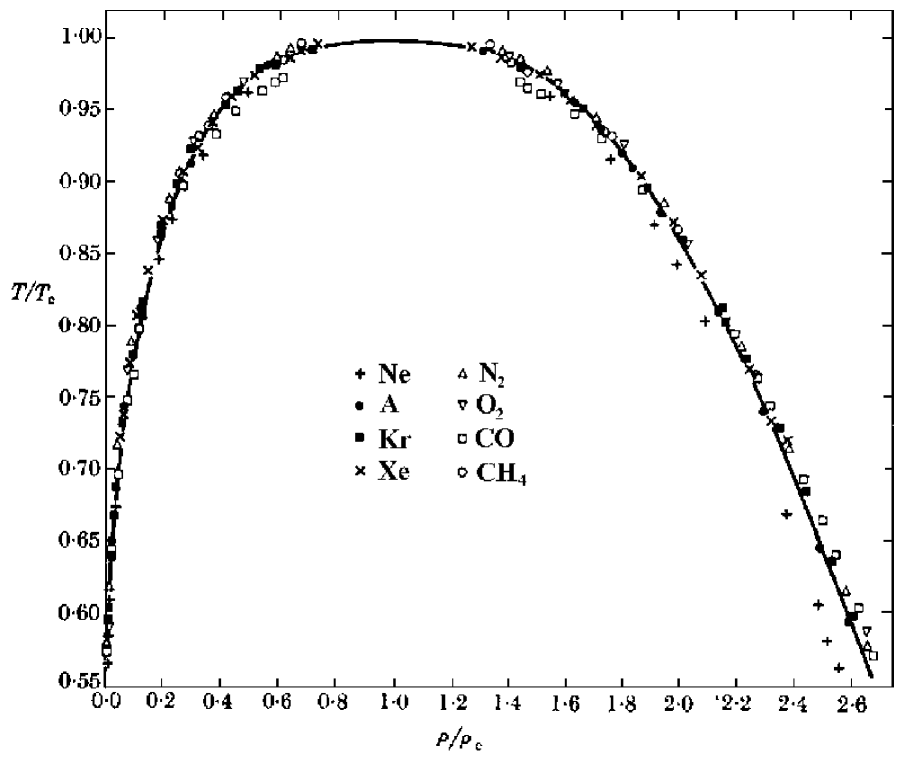
Figure 14: Phase diagram showing a first order transition for eight fluids indicated on the figure [192]. The collapse of the coexistence curve shows the universality character of the phenomenon.

For instance for a fluid system one observes that the specific heat at constant volume $C_{V}$ behaves like $C_{V}\sim|t|^{-\alpha}$, the liquid-vapor density difference $(\rho_{l}-\rho_{g})\sim(-t)^{\beta}$, the isothermal compressibility $K_{T}\sim|t|^{-\gamma}$ and the correlation length $\xi\sim|t|^{-\nu}$, where all the indices are positive. The interest in the knowledge of critical exponents lies in the fact that they possess a universal character. While the location of the critical exponent itself may depend on the details of the interparticle interaction, the exponents are universal in the sense that they depend only on quantities like the dimensionality $d$ of space and the symmetry properties of the order parameter. Evidence for this has been verified number of times, in particular for the first time by Guggenheim [192] in the phase separation line of the liquid-gas transition for different species, see Fig. 14, for which it can be seen that the exponent $\beta=1/3$. The very same value for $\beta$ comes in the 3-dimensional Ising model, the magnetization $M$ at $T=T_{c}$ behaves like $\simeq(-t)^{1/3}$. These properties lead to define universality classes for systems showing the same behaviour at phase transitions. They allow to classify a priori very different physical systems by means of their critical exponents which characterize the behaviour of their order parameters at a critical point. Scaling relations which govern the behaviour of physical quantities when one looks at systems at different scales allow to establish inequality or equality relations between the exponents. This has already been shown in section 4 in the framework of percolation, see also below.

The importance of critical exponents raises the question of their explicit determination. Generally this can only be done numerically. Since critical exponents only make sense in infinite systems it is necessary to find methods which lead to an extrapolation of the behaviour of the critical observables to the infinite limit in order to determine them. There exists different, more or less sophisticated methods and numerical techniques which allow for very precise determinations of exponents, see f.i. refs. [193, 194].

A whole class of methods relies on the so called finite size scaling assumption (FSS). The scaling hypothesis implies that in the neighbourhood of a critical point a system shows self-similarity properties when it is examined at different scales. These properties are reflected in the mathematical behaviour of thermodynamic functions and physical observables which show so called homogeneity properties, i.e.

$$f(ab)=f_{1}(a)f_{2}(b)$$

where $f_{1}(a)=a^{p}$, $p$ is a real number, and for an arbitrary number of variables

$$f(\lambda x_{1},\lambda x_{2},\ldots\lambda x_{n})=\lambda^{p}f(x_{1},x_{2},\ldots x_{n})$$

If, for the case of two variables, one chooses $\lambda=x_{1}^{-1}$ then

$$f(x_{1},x_{2})=x_{1}^{p}f(1,x_{2}/x_{1})=x_{1}^{p}g(x_{2}/x_{1})$$

which shows that in practice $F$ does not depend on the two independent variables $x_{1}$ and $x_{2}$, but on $x_{1}$ and the ratio $x_{2}/x_{1}$ whatever $x_{2}$. For fixed $x_{1}$, $g$ is a scale independent function of $x_{2}/x_{1}$, $g(\lambda x_{2}/\lambda x_{1})=g(x_{2}/x_{1})$. The FSS assumption allows to relate the behaviour of an observable at some scale to its behaviour at another scale.

As an example of application consider an observable $O_{L}(\Delta t)$ which depends on a variable $\Delta t=(t_{c}-t)/t_{c}$ where $t=t_{c}$ is a critical point of the infinite system and describes a finite system of linear dimension $L$. If one defines $x(L,t)=\xi_{L}(t)/L$ where $\xi_{L}(t)$ is the correlation length in the finite system for a fixed value of t in the neighbourhood of $t_{c}$, FSS stipulates that [195]

$$O_{L}(\Delta t)=O(\Delta t)Q_{0}\big{(}x(L,t)\big{)}$$ (27)

where $O(\Delta t)$ corresponds to the value of the observable in the corresponding infinite system and $Q_{0}\big{(}x(L,t)\big{)}$ is a scaling function which is universal in the sense that it does not depend on $t$ but only on the ratio $x$ in the neighbourhood of $t_{c}$, i.e. all points corresponding to different $t$’s lie on the same curve when $Q_{0}$ is plotted as a function of $x$. If $O_{L}(\Delta t)$ converges to a finite $O(\Delta t)$ with increasing $L$, $Q_{0}(x)$ can be determined from (27) and close to $t_{c}$ one expects that

$$O(\Delta t)=O_{L}(\Delta t)/Q_{0}(x)\sim(t_{c}-t)^{-\alpha}$$ (28)

if $O$ shows a critical behaviour, and $\alpha$ is a critical exponent. If $Q_{0}(x)$ can be obtained numerically it is generally fitted to a polynomial in $x$

$$Q_{0}(x)=1+b_{1}x+b_{2}x^{2}+\cdots$$

with $Q_{0}(0)=1$ if $\xi_{L}(t)/L$ goes to zero when $L$ goes to infinity. This type of methods has been applied in different places, in particular to percolation $(t\equiv p)$ and spin systems [195, 196, 197]. Their use leads generally to reliable and accurate values of $t_{c}$ and critical exponents. Their practical implementation shows however that the numerical determination of these quantities can be a cumbersome task. Other methods have been proposed by different authors [198, 55], in particular in order to fix the exponents which describe experimental fragment size distributions in the vicinity of the expected critical point where the distribution should follow a power law in the corresponding infinite system. However these methods rely on expressions which are valid for large systems and do not extrapolate to the thermodynamic limit. Even though the information on criticality extracted this way looks reasonable it remains suspicious to use it in order to conclude about the determination of the universality class of the phase transition which is the ultimate goal of such an analysis. On the other hand, it is difficult to believe that the use of scaling assumptions implemented by means of FSS can be used in practice in the framework of the analysis of experimental events since, among other severe problems, the number of points necessary to construct scaling functions would be rather restricted because of the small interval of sizes which can be reached with nuclei.

Critical exponents are rather refined quantities. There remains hope to be able to detect the existence and eventually the order of phase transitions in nuclear matter by other means. Considering thermodynamic aspects of fragmentation, this can possibly be reached restricting ones considerations to finite systems. The question concerning the order of a phase transition has been raised recently on theoretical grounds [199, 200] in the framework of the Lee and Yang theory [201] and the approach of Grossmann and collaborators [202]. The criterion which allows to distinguish between different orders concerns the location of the zeroes of the grand canonical and the canonical partition function in the complex temperature plane. But these considerations are theoretical, possibly difficult to implement in practice for interacting systems and the connection with experiment is lacking. In section 6 we shall show that there may exist simple operational means to overcome the problem.

Finite size effects can hide or even delude the truth with respect to the order of a phase transition. Different ensembles may lead to a different behaviour of observables when applied to finite systems. We shall indeed see below that characteristic features of observables when calculated in the framework of a specific ensemble may be of some help in order to decide about the nature of the transition. The assertion has however again to be taken with a grain of salt since there does not exist any guarantee that these characteristic features will maintain their validity in the thermodynamic limit.

5.2 Lattice models

We present and discuss here different lattice models which have been introduced and studied by different groups. The essential point of interest concerns the existence of signs for the existence of one or several phase transition(s) in nuclear matter.

5.2.1 The Ising model as a random cluster model

The success of percolation raised the question for the reasons of its achievements. As we saw in section 4, classical lattice systems described by the Ising, Ashkin-Teller and Potts models are generally close to percolation models [161, 162]. They describe Hamiltonian systems, hence they introduce an explicit, physical description of an $N$-body system. This was the main motivation for the introduction of the Ising model in order to interpret the cluster size distributions of an excited, fragmented system [169, 203].

In order to be able to get a clearer understanding of the behaviour of observables the model was first studied in $d=2$ which allows the use of analytical techniques [169]. The Hamiltonian reads

$$H=-J_{1}\sum_{n=1}^{N}\sum_{m=1}^{M}\sigma_{nm}\sigma_{n+1m}-J_{2}\sum_{n=1}^{N}\sum_{m=1}^{M}\sigma_{nm}\sigma_{nm+1}$$

where $J_{1}$ and $J_{2}$ are positive constants and $\sigma_{nm}$ is a classical spin $(=\pm 1)$ located at the position $(n,m)$ on a $2d$ lattice with $N$ lines and $M$ columns.

An ensemble of sites are said to form a cluster if the corresponding spins show the same value and each site of the cluster has at least one neighbour site with a spin of the same value (connexity). The perimeter of a cluster is the ensemble of nearest neighbour sites whose spin takes the value which is opposite to the spins in the cluster. With this definition and after a mapping of the classical system into a quantum system of independent fermions [204] it is convenient to introduce projection operators along lines $(l)$ and columns$(c)$

$$P_{+}^{(l)} = \frac{1}{2}(\textrm{\bf{\large 1}}+\sigma_{nm}^{x}\sigma_{nm+1}^{x})$$

$$P_{+}^{(c)} = \frac{1}{2}(\textrm{\bf{\large 1}}+\sigma_{nm}^{x}\sigma_{n+1m}^{x})$$

and

$$P_{-}^{(l)} = \frac{1}{2}(\textrm{\bf{\large 1}}-\sigma_{nm}^{x}\sigma_{nm+1}^{x})$$

$$P_{-}^{(c)} = \frac{1}{2}(\textrm{\bf{\large 1}}-\sigma_{nm}^{x}\sigma_{n+1m}^{x})$$

where $\sigma^{x}$ is the standard Pauli matrix. The correlation operators $P_{+}$ and anticorrelation operators $P_{-}$ have a classical interpretation, $P_{+}^{(l,c)}=1$ and $P_{-}^{(l,c)}=0$ for aligned spins, and $P_{+}^{(l,c)}=0$ and $P_{-}^{(l,c)}=1$ for anti-aligned spins.

These operators allow to define the probability of presence of a cluster of a given size and geometry.

$$\Pi^{(i)}=<P_{+}^{L_{+}^{(i)}}\cdot P_{-}^{L_{-}^{(i)}}>$$ (29)

where the index $i$ characterizes the linked cluster which is considered, $L_{+}^{(i)}$ is the number of bonds between cluster sites and $L_{-}^{(i)}$ the number of bonds between the surface of the cluster and the perimeter sites. For a given cluster size $N_{S}$, one finds

$$2L_{+}^{(i)}+L_{-}^{(i)}=4N_{S}$$

The brackets in (29) indicate a trace over the many-body quantum states [169].

The multiplicity corresponding to clusters of a fixed number of sites $N_{S}$ and a fixed topology $(i)$ is given by

$$M^{(i)}(N_{S})=D^{(i)}(N_{S},N_{T})\Pi^{(i)}$$

where $D^{(i)}(N_{S},N_{T})$ is the degeneracy of cluster of size $N_{S}$, and $N_{T}$ is the total number of sites. The total multiplicity of clusters of size $N_{S}$ reads

$$\overline{\mathcal{M}}(N_{S})=\sum_{(i)}M^{(i)}(N_{S})$$

Since the number of spins with a given sign is not fixed in the model (see discussion below) one introduces a normalization factor $\mathcal{N}$ and

$$\overline{M}(N_{S})=\frac{1}{\mathcal{N}}\overline{\mathcal{M}}(N_{S})$$

such that

$$N_{T}=\mathcal{N}\sum_{N_{S}=1}^{N_{T}}N_{S}\overline{\mathcal{M}}(N_{S})$$

The interest of this approach lies in the fact that it is easy to work out the evolution of quantities like the average size of clusters as a function of the temperature

$$<N_{S}(T)>=\sum_{N_{S}=1}^{N_{T}}N_{S}\overline{M}(N_{S},N_{T})/\sum_{N_{S}=1}^{N_{T}}\overline{M}(N_{S},N_{T})$$

the corresponding variance

$$\sigma^{2}(T)=<N_{S}^{2}(T)>-<N_{S}(T)>^{2}$$

and the fragment size distributions. The expected qualitative features obtained in a finite system when the temperature of the system increases is observed. The results can be interpreted in terms of site percolation concepts. “Occupied” sites in the percolation framework correspond to cluster sites in the present case and “empty” sites to perimeter sites. The relative amount of “occupied” sites is governed by the temperature. The number of perimeter sites increases with increasing temperature and the relative amount of large clusters diminishes. In the percolation picture the number of empty sites increases with decreasing occupation probability $p$, leading to the same trend.

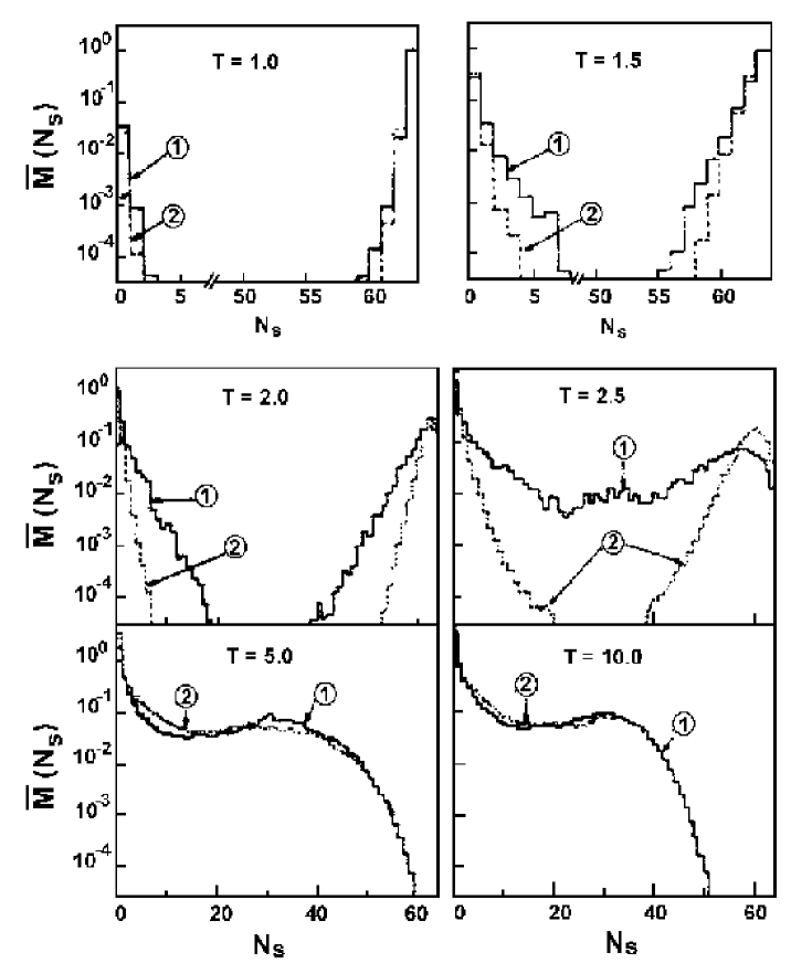
Figure 15: Multiplicities of clusters made of parallel spins in the Ising model for (1) short range and (2) long range interactions and different temperatures [203].

The model which deals with short range nearest neighbour interactions has been extended to include long range interactions [203]. Numerical studies show that the range of the interaction in finite systems does not change the qualitative behaviour of multiplicity distributions in finite systems, except for the fact that a long range attractive interaction favours the survival of large clusters over a large temperature interval. At high temperature both distributions collapse onto each other, as it can be seen in Fig. 15. The presence of “critical” events is seen in the behaviour of the second moment of the cluster size distribution. Similar results are obtained with $3d$ systems. The a priori general difficulty to relate lattice models with nuclear fragmentation will be discussed later. The use of the Ising model presents a further weakness which stems from the fact that the identification of clusters in terms of spins which are aligned in a given direction breaks the $\mathcal{Z}_{2}\ (\pm 1)$ symmetry which is present by construction and leads to non conservation of the number of “particles”. The remedy to this disease consists of the introduction of a term governed by a Lagrange multiplier. We shall come to this point below.

The present models were thought to build up a bridge between the purely geometrical concepts introduced by percolation models and sophisticated liquid-gas descriptions. They triggered the construction of more refined models aimed to describe and understand the physics of fragmentation and critical behaviour in finite nuclei.

5.2.2 The grand canonical lattice gas model (LGM)

The preceeding study was aimed to look for the connection between the geometrical and probabilistic concepts which define percolation models and the thermodynamic properties of spin models which are defined in terms of classical Hamiltonians. It did however not explicitly define the link between bond probabilities, energy and temperature.

This link was established by Jicai Pan and Das Gupta [205, 206, 207] and Campi, Krivine and collaborators [208, 209, 210]. In ref. [208] the authors consider a classical lattice gas model defined by the Hamiltonian

$$H=\sum_{i=1}^{N}n_{i}\frac{p_{i}^{2}}{2m}-\epsilon\sum_{<i,j>}n_{i}n_{j}$$

where $n_{i}=0,1$ is the occupation number of the lattice site $i$, $N$ the total number of lattice sites and $\epsilon$ the energy between nearest neighbours $<i,j>$. The number of particles $A=\sum_{i}n_{i}$ is conserved in the average by means of a constraint induced by a Lagrange multiplier procedure.

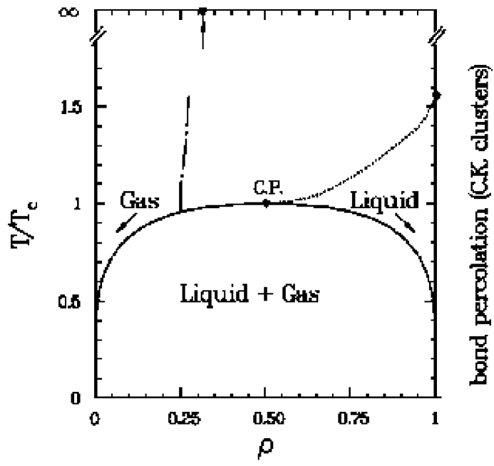
Figure 16: Typical phase diagram corresponding to a lattice gas model [208]. See discussion in the text.

The model is treated by means of Metropolis Monte Carlo simulations, in the framework of the grand canonical ensemble which can be formally related to the canonical description of the Ising model with magnetic field [211]. The exploration of the properties of the system in the density-temperature plane $(\rho,T)$ leads to the typical phase diagram shown in Fig. 16. One observes the presence of a full line which separates two phases above the line, a gas at low $\rho$ and a liquid at large $\rho$. Below the separation line gas and liquid coexist in an inhomogeneous phase forming domains (clusters) of different sizes. In the thermodynamic limit the transition line corresponds to a first order transition. At $\rho=1/2$ in units of the normal density $\rho_{0}$ there appears a critical point at $T=T_{c}$ which corresponds to a continuous transition characterized by critical exponents which are universal, i.e. do not depend on the detail of the interaction between particles.

The main point of interest in the study of this model lies in the analysis of the cluster content of the system for different values of $\rho$ and $T$. The identification of clusters raises the question of their definition. One gets confronted with two problems [208]. The most disturbing one concerns the fact that the thermodynamic critical point does not coincide with the percolation critical point at which the cluster size distribution shows a power law behaviour if clusters are defined as an ensemble of particles occupying connex (nearest neighbour) sites [212]. If clusters are defined in a purely geometric way as made of connected occupied sites percolation events generate a whole line of points in the phase diagram, an infinite cluster is obtained in the infinite limit on the right hand side of the dot-dashed line shown in Fig. 16. This is of course unphysical, since at high temperature one expects essentially small clusters and isolated particles. A remedy to this problem was proposed by Coniglio and Klein [213] who introduced the energy concept in order to define clusters as made of connected ensembles of nearest neighbour particles with a bond probability smaller or equal than

$$p_{CK}(\epsilon/T)=1-exp(-\epsilon/2T)$$ (30)

If one uses this definition the thermodynamic and percolation critical point coincide and there exists a whole continuous line of points in the $(\rho,T)$ plane called the Kertész line [214], along which the cluster size distribution shows a power law behaviour. The important point concerns the fact that the definition (30) is shown to be very close to the bond probability prescription between neighbour particles given by

$$p_{b}\bigg{(}\frac{\epsilon}{T}\bigg{)}=Prob\bigg{[}\bigg{(}\frac{p^{2}}{2m}-\epsilon\bigg{)}<0\bigg{]}=1-\frac{4}{\sqrt{\pi}}\int_{\sqrt{\epsilon/T}}^{\infty}\mathrm{d}u\,u^{2}e^{-u^{2}}$$ (31)

which stipulates that a pair of particles is bound if $(p^{2}/2m-\epsilon)<0$ where the momentum $p$ is drawn from a Maxwell distribution [206, 208]. It is shown [208] that if (31) is chosen as a bond criterion then the separation energy $S(A)$ of one particle from a bound cluster of $A$ particles satisfies approximately the inequality

$$S(A)=B(A-1)-B(A)<0$$

where $B(i)$ is the binding energy of a system of $i$ bound particles, and the “critical” percolation line coincides approximately with the Kersétz line defined above.

Following this prescription one obtains cluster size distributions in different part of the $(<\rho>,T)$ plane, where $<\rho>$ is the average density in the grand canonical ensemble. These distributions show the same properties as those obtained in the framework of percolation models, i.e. a power law behaviour corrected for finite size effects along the Kersétz line, with a power law exponent $\tau\simeq 2.2-2.3$, an exponential decay at low density and high temperature, the characteristic large cluster peak at high density. One may notice also that contrary to the case of multifragmentation models [79, 110] in which clusters are by construction spherical the cluster along the Kersétz line have surfaces with fractal properties which allows for a freeze-out density larger than the “critical” density. Furthermore one observes that the excitation energy per particle above the ground state keeps approximately constant along the critical line [210]. Further work relying on lattice models in the framework of nuclear fragmentation was developed in the recent past. It concerns the study of the two types of phase transitions (thermodynamic and percolation) mentioned above which may be of different orders (first and second), the importance of the Coulomb interaction, problems related to the finite nature of the systems. We examine different approaches and their contribution to the understanding and explanation of these questions in the next subsections.

5.2.3 Lattice models and their application in the framework of nuclear fragmentation

The generic character of lattice gas models (LGM), their kinship with percolation models and classical systems of particles with short range interactions lead to a large amount of theoretical investigations.

Das Gupta and Jicai Pan proposed different variants of this type of models [205, 206] and applied them for direct comparison with experimental data [207]. They worked out the canonical partition function $\mathcal{Z}$ on the lattice in an analytic form by using the Bragg-Williams approximation for the calculation of the potential contribution to the free energy. In this approximation the number of sites which are occupied in the neighbourhood of a fixed ocupied site is fixed in the average as $zn/N$, where $z$ is the number of neighbours (coordinance) and $n/N$ the average number of occupied sites ($n$) in a lattice with $N$ sites. The approximate analytical expression of $\mathcal{Z}$ allows to determine different equations of state, in particular the relation between the pressure and the volume which comes out as a van der Waals-type equation [205]. In a further development [206] the authors introduced a grand canonical description, the mean field Bragg-Williams approximation was replaced by the Bethe-Peierls approximation which corresponds to the introduction of blocks of lattice sites inside which occupied nearest neighbour sites interact. An interaction $\overline{\epsilon}$ between blocks is taken into account and fixed along with the chemical potential of the particles by means of a self-consistent procedure. This further improvement brings in fact rather small changes when compared with the Bragg-Williams approximation and is rather close to the outcome of a mean field approach using a realistic Skyrme interaction. In all cases the descriptions show signs for the existence of a first order phase transition for all values of $\rho$, a second order transition at $\rho_{c}=0.5\rho_{0}$ where $\rho_{0}$ is the normal nuclear matter density.

Emphasis was put on the study of the cluster content of finite lattice gas systems. It was shown by means of explicit calculations that the second moment of the fragment size distribution shows a maximum at different values of the temperature for different values of the density [205]. In an interpretation in terms of percolation concepts this is the sign for the existence of a Kertész line. If one introduces

$$p^{2}_{r}/2\mu-\epsilon \leq 0$$

or $$> 0$$

(where $p_{r}$ is the relative momentum between neighbouring particles, $\mu$ the reduced mass and $\epsilon$ the strength of the interaction) as a criterion to decide whether the considered particles are bound or not the bond probability is the same as the one given by (31) in section 5.2.2 [206]. Effective exponents $\tau$ extracted from the experiment in the spirit of refs. [21, 22] (see section 2.1) were compared with lattice calculations in an attempt to obtain informations about characteristic freeze-out densities of systems formed at different beam energies. The freeze-out density determined in this way came out to be $\rho\simeq 0.4\rho_{0}$.

One very important point in nuclear fragmentation concerns the role and importance of the Coulomb interaction. This point has been emphasized in the framework of multifragmentation models [79]. A calculation in the framework of an LGM for a large system obtained through the collision of $Au$ on $Au$ shows that the Coulomb interaction may have a sizable effect and may lead to large discrepancies between LGM and the experiment [207]. One may introduce two types of binding energies between nearest neighbours which correspond to the interaction between identical and different types of particles (protons and neutrons) [215]. This has been done by means of Monte Carlo simulations and the results were compared to the outcome of molecular dynamics (MD) calculations which coincide with the lattice gas results in the absence of the Coulomb interaction. It is no longer the case when this interaction is taken into account. The LGM results deviate from the MD results in large systems with a sizable amount of protons. We shall come back to the Coulomb problem below.

Further comparisons with different models have been performed [216] such as percolation and multifragmentation models. The analysis of different observables shows that these models share common features, in particular the statistical multifragmentation and lattice gas approaches, except for quantities like the specific heat $C_{V}$ at low temperature. The multifragmentation approach possesses quantum mechanical properties and $C_{V}$ increases linearly with $T$ while in the LGM $C_{V}$ stays at the constant value $3/2$. It should be mentioned that the algorithm used in the simulations [205, 206, 207] does not sample the events in a rigorous fashion [217]. This should however not qualitatively affect the results and change the conclusions.

5.2.4 Extensions of the LGM in the framework of the canonical ensemble

Lattice gas models were further developed and analysed in the framework of the canonical ensemble by Gulminelli and Chomaz [218, 219, 220, 221], Borg, Mishustin and Bondorf [222] and Carmona, Richert and Tarancón [197].

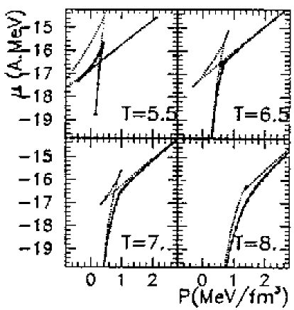
Figure 17: Exact (full lines) and mean field (dotted lines) chemical potentials as a function of pressure for different temperatures [223].

Gulminelli and Chomaz [218, 220] constructed the phase diagram of a finite system by working out the compressibility coefficient. This quantity shows an anomalous behaviour, it becomes negative at some temperature $T$ over some density interval, the sign for the existence of a first order phase transition in the infinite system. Fig. 17 shows the behaviour of the chemical potential represented as a function of pressure exemplifies this phenomenon. It has also been observed that the fragment size distribution possesses a separation line (Kertész line) which crosses the phase separation line and enters the coexistence zone at some low value of the density. This is a priori somewhat surprising since it means that in the thermodynamic limit one would observe the existence of a second order transition in the coexistence zone. However, it is found out that for large systems the separation line stops effectively at the thermodynamic critical point located at $\rho/\rho_{0}=0.5$, hence the authors interpret the effect as a typical finite size effect. They comfort this point of view by showing that in this region of the phase diagram the fragment size distribution does not go through a power law distribution when one crosses the separation line in the coexistence zone. If this is so, it means that the system never shows the signs for a critical behaviour for subcritical densities.

Lattice gas models were also recently extended to the case where two types of particles, protons ($p$) and neutrons ($n$) coexist. The refinement is implemented by the choice of different nearest neighbour interaction strngths, $\epsilon_{np}\neq\epsilon_{nn}=\epsilon_{pp}$. These constant quantities were chosen such as to reproduce the nuclear binding energies of the corresponding quantum systems. One may ask for the consequences of the introduction of the isospin degree of freedom [219]. In fact, the extension of the model has only a small effect on the phase diagram, so that in practice there exists only one relevant order parameter, $\rho_{L}-\rho_{G}$, where $\rho_{L}$ and $\rho_{G}$ are the liquid and gas density respectively. Critical exponents do not depend on the isospin degree of freedom either, and the critical temperature shows a quadratic dependence on asymmetry. The sign for isospin effects may perhaps be found in the fact that in the coexistence region the vapour mode of small fragments is more isospin asymmetric than the liquid mode of larger fragments. This can in fact be observed in the experiment [268, 269].

A similar model with protons and neutrons has been studied in ref. [222]. The thermodynamic properties of the system are determined for open boundary conditions and the caloric curve is constructed at constant density and constant pressure. For fixed pressure one observes clearly the appearance of a plateau which is the sign for a first order transition. For fixed density, the caloric curve is monotonously increasing with energy. Fragment size distributions are analysed along isobars and isochores. They show the usual trend, with increasing temperature the large fragment yield shrinks and the small fragment and light particle contribution increases continuously.

Recently the effect of the shape of the surface of the fragmenting system on the fragment size distribution has also been investigated [221]. Cubic shapes with and without periodic boundary conditions as well as spherical shapes with sharp and diffuse surfaces have been considered. These shapes have no real influence on the thermodynamic properties and fragment size distributions of small systems with typically $100$ particles at the critical density. Similar tests have been performed on other models, see below [224]. It raises the question wether the shape dependence of fragmentation events may be detected in experimental data.

5.3 Cellular models of nuclear fragmentation

As already mentioned the success of percolation concepts for the reproduction of experimental fragment size distributions raised the question of the correlations between theses quantities and the actual dynamics of highly excited nuclei [169, 203]. Peripheral collisions [225] indicate that the spectator remnant behaves essentially as an excited system of particles which is thermalized. It leads to the idea that fragmenting nuclei can essentially be described as completely disordered systems of interacting particles, at least under the experimental conditions described above. Furthermore, it is a non trivial but established fact that disorder may be connected with complexity and universality [226]. This property reflects the fact that disordered systems are not sensitive to the details of their dynamical characteristics but show features which are common to many of them such as the scaling properties discussed above.

In the present section we introduce and discuss so called cellular models which are aimed to relate the phase space properties of a classical system of particles to bond probabilities and hence to the generation of bound clusters. They can be considered as extensions of lattice models.

5.3.1 Disordered systems and cluster identification

A fragmenting nucleus is considered as an assembly of interacting particles contained in a finite three dimensional volume $V$ divided into $A$ cubic cells, $V=Ad^{3}$ where $d$ is the linear size of each cell. Each cell contains one particle [224, 227]. Each particle inside its cell is characterized by its position $\vec{r}_{i}\,(i=1,\ldots,A)$ and linear momentum $\vec{p}_{i}$, both phase space coordinates being taken at random and obeying $|\vec{r}_{i}-\vec{r}_{j}||\vec{p}_{i}-\vec{p}_{j}|\geq\hbar$ which has to be verified for particles located in neighbouring cells. The interaction is chosen as a short range two-body potential adapted to a classical description of the nucleus [228, 229]. It acts between nearest neighbours only. The total energy of two such particles can be split into a centre of mass and a relative contribution

$$E=P^{2}/2M+p^{2}/2\mu+V(r)=P^{2}/2M+\epsilon$$

with $\vec{P}=\vec{p}_{i}+\vec{p}_{j},\,\vec{p}=\vec{p}_{i}-\vec{p}_{j},\,r=|\vec{r}_{i}-\vec{r}_{j}|,\,M=2m$ and $\mu=m/2$, where $m$ is the mass of the nucleon. Each coordinate $\vec{r}_{i}$ is defined as $x_{i}=x_{i0}\pm\eta d/2$ (same for $y_{i}$ and $z_{i}$), where $x_{i0}$ locates the centre of the cell and $\eta$ is drawn uniformly in the interval $[0,1]$. The momenta $\{\vec{p}_{i}\}$ are taken uniformly in a sphere of radius $p_{max}$. Two neighbouring particles are said to be bound to each other if $\epsilon<0$ and unbound if $\epsilon>0$. By means of numerical simulations the criterion allows to construct a bond probability $p(E)=n(E)/\mathcal{N}(E)$ where $\mathcal{N}(E)$ is the total number of draws in an energy interval $[E,E+\delta E]$ and $n(E)$ the total number of events out of $\mathcal{N}(E)$ for which the two-particle system is bound at energy $E$. The violation of the inequality relating relative distances and momenta defined above leads to the rejection of the corresponding event.

Three different procedures have been introduced in order to identify bound clusters. In the first called A2, the energy $E$ of each pair is drawn from the distribution $\mathcal{N}(E)$ and the corresponding $p(E)$ is compared to a random number $\eta$ belonging to $[0,1]$. If $p(E)>\eta$ the pair is considered as bound and unbound in the reverse case. This procedure is close to a percolation algorithm but $p(E)$ is not chosen in a uniform distribution. It neglects also the correlations which exist between pairs sharing common particles.

The second procedure (A1) fixes the energy of a pair $E=E(\vec{r}_{i},\vec{p}_{i};\vec{r}_{j},\vec{p}_{j})$ of neighbouring particles $i$ and $j$ by means of their phase space coordinates which are fixed as described above. This fixes also $p(E)$ and the bond criterion is the same as for A2. Finally, correlations are fully taken into account by means of algorithm A0 for which the generated phase space $\{\vec{r}_{i},\vec{p}_{i},i=1,\ldots,A\}$ is used to calculate explicitly $\epsilon$ for each pair. It corresponds to a deterministic determination of the clusters for each generated event.

It is important to notice that none of these descriptions implies that the considered systems are necessarily in any kind of equilibrium.

5.3.2 Physical observables. Confrontation with bond percolation

The fragment content can be characterized by the mass distribution, its moments and associated observables like $\gamma_{2}$ which has already been defined above. In order to compare directly with the experiment these observables are determined as a function of the multiplicity $m$ which can be measured and is univoquely related to the bond probability $p$. For each event $k$

$$m_{2}^{(k)} = {\sum_{i}}^{\prime}\,i^{2}P_{i}^{(k)}(m)$$

$$\textrm{or}\quad S_{2}^{(k)}(m) = m_{2}^{(k)}(m)/m_{1}^{(k)}(m)$$

where $P_{i}^{(k)}(m)$ is the number of clusters of size $i$ and the prime index indicates that the heaviest fragment is omitted. Similarly

$$\gamma_{2}^{(k)} = m_{0}^{(k)}(m)\cdot m_{2}^{(k)}(m)/m_{1}^{(k)^{2}}(m)$$

$$= 1+\sigma^{(k)^{2}}(m)\cdot m_{0}^{(k)^{2}}(m)/m_{1}^{(k)^{2}}(m)$$

$$\textrm{where}\quad\sigma^{(k)^{2}} \equiv \bigg{(}m_{0}^{(k)}(m)\cdot m_{2}^{(k)}(m)-m_{1}^{(k)^{2}}(m)\bigg{)}/m_{0}^{(k)^{2}}(m)$$

Average quantities are defined as

$$<m_{2}(m)> = N_{ev}^{-1}\sum_{k=1}^{N_{ev}}m_{2}^{(k)}(m)$$

$$<\gamma_{2}(m)> = N_{ev}^{-1}\sum_{k=1}^{N_{ev}}\gamma_{2}^{(k)}(m)$$

Numerical investigations have first been performed with the algorithm A2. The comparison with bond percolation is shown in Fig. 18. One observes an amazing agreement between the two descriptions although bond probabilities are taken from different distributions and this agreement is very robust with respect to the strength of the two-body potential. In fact, if $\rho(\eta)$ is the probability distribution of $\eta=p(E_{0})$ for a given $E_{0}$ the equivalent probability in bond percolation is

$$\tilde{\eta}=1-\int_{0}^{\eta}\mathrm{d}\eta^{\prime}\rho(\eta^{\prime})$$

Through this relation $m$ and $\tilde{\eta}$ are related to each other in the same way as $m$ and $p$ in bond percolation. In particular, one observes a critical value $\tilde{\eta}_{c}$ for which an infinite cluster appears in the infinite system.

The agreement survives also if protons and neutrons are differentiated by means of different bond probabilities $p_{pp}(E)=p_{nn}(E)\neq p_{pn}(E)$ [224]. Qualitatively similar but quantitatively different results are obtained with algorithm A1, in particular the location of the maxima of $<m_{2}>$ and $<\gamma_{2}>$ are shifted to higher values of $m$. The deviations are indicated by the correlations which are built in A1 and absent from A2. One expects that the effect is due to the hybrid nature of the algorithm which mixes probabilistic and deterministic properties.

Algorithm A0 provides a priori the most realistic description since it takes all correlations consistently into account. It allows also for an easy treatment of the long range Coulomb interaction. For a fixed value of the length $d$ of the cubic cells the moments $<m_{2}>$ and $\overline{\gamma_{2}}=<m_{2}>\cdot<m_{0}>/<m_{1}>^{2}$ can differ sensibly from the percolation results. If, however, one averages over events corresponding to values of $d$ which are uniformly distributed over a given interval of densities $\rho$, say from $5\times 10^{-3}$ to $0.17\,fm^{-3}$, one obtains mass distributions, $<m_{2}>$ and $\overline{\gamma_{2}}$ which are remarkably close to those obtained with A2 and robust with respect to modifications of the strength of the short range potential as it is the case with A2. The agreement between the results obtained with A0 and A2 is not easy to understand. It seems to indicate that averaging over densities acts as a mean to wash out correlation effects.

5.3.3 Confrontation with experimental data

Multifragmentation data available from experiments made by the ALADIN collaboration [230, 178, 231] have been confronted with the outcome of the A2 algorithm in the same way as it was done for the percolation approach in section 4.7 [224, 227]. The charge $Z$ to mass $A$ relation used is the same as in this section. For fragments of mass $A=3$ the isobaric ratio ${}^{3}H/^{3}He$ is fixed to $2.2$. The mass of the spectator part of the fragmented system depends on the impact parameter, the number of particles involved is divided into $10$ different sets corresponding to $10$ intervals for the impact parameter. Each system with $A_{i}\,(i=1,\ldots,10)$ particles is put in a cube of $7^{3}$ cells in as compact and symmetric a geometry as possible. Each calculated observable $O$ is averaged over the whole impact parameter range

$$<O>=\sum_{i=1}^{10}b_{i}\Delta b_{i}O(b_{i})\ \bigg{/}\sum_{i=1}^{10}b_{i}\Delta b_{i}$$

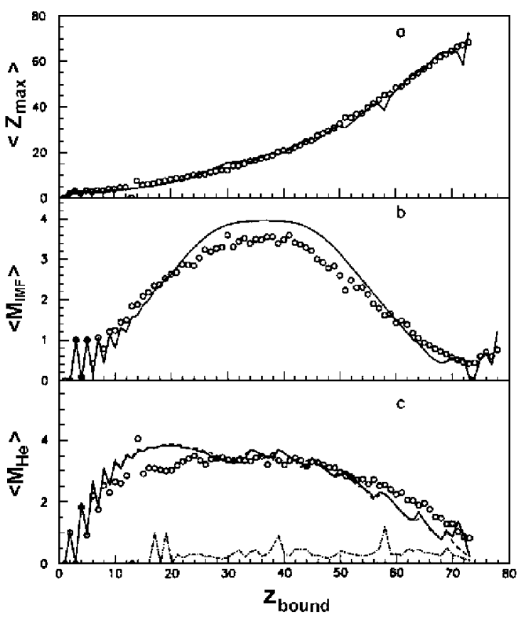
Figure 19: Different observables represented as a function of $Z_{bound}$. The experimental average largest cluster $<Z_{max}>$, IMF multiplicities $<M_{IMF}>$ and $He$ multiplicities $<M_{He}>$ represented by dots are compared to calculations performed with the A0 algorithm, see text [224].

Results of this analysis are shown in Fig. 19 for different observables, the average value of the charge of the largest fragment $Z_{max}$, the IMF $(3\leq Z\leq 30)$ multiplicity, the $He$ isotope multiplicity which are represented as a function of $Z_{bound}$ and the average number of fragments with charge $6\leq Z\leq 30$. As it can be seen, the agreement between experiment and simulations is excellent. This is not really surprising since bond percolation and A2 lead to very close results and, as it has been seen in section 4, percolation reproduces experimental results.

5.3.4 Geometric and collective effects

The use of simple cubic shapes for the description of the fragmenting system may appear as too restrictive. This point has been investigated by introducing other shapes, spheres, parallelepipeds, streaked, crenellated and crumpled surfaces which were generated by means of a random growing process leading to fractal surface structures which may introduce empty cells in the bulk of the system [224]. The moments of the mass distributions show deviations from the cubic case, but these deviations are always surprisingly small, they never lead to qualitative changes in any observable related to fragment size distributions.

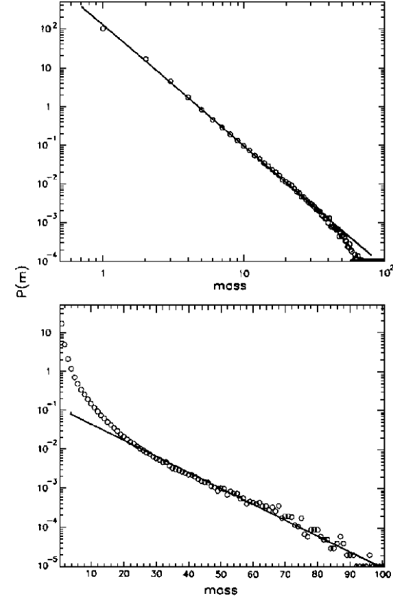
Figure 20: Mass distributions for a $6^{3}$ system. The upper curve corresponds to a calculation using the A0 algorithm, the lower corresponds to the simulation of collective effects, see text [224].

Cellular models describe disordered systems which show a power law behaviour with deviations due to finite size effects at a value of the fragment multiplicity corresponding to criticality in the infinite system. Experimentally this situation prevails for peripheral collisions [230, 178, 231]. In the case of more central collisions fragment size distributions show rather an exponential fall off as a function of the mass number [232]. These collisions are also characterized by a sizable collective radial flow [233, 155]. It is out of scope to reproduce this dynamic effect with the present simple-minded approach. It is however possible to mimic it. This was done with algorithm A0, mixing events with linear cell size $1.8\leq d\leq 6\,fm$ for $A=216$ particles. The linear momenta strengths of the particles are chosen randomly but their directions are fixed along a line which joins the centre of the system to their actual position, pointing out of the system. The typical behaviour of the mass distribution in this case is shown in Fig. 20, along with the case where collective effects are absent. The shape which is power law like in the case where the directions of the momenta are random gets very close to an exponential for sizes between $20$ and $90$ units of mass. Deviations are observed for light and heavy fragments. Such a behaviour has been confirmed in ref. [155] were a more detailed analysis on a more sophisticated approach has been performed. This result comforts the idea that peripheral collisions induce the generation of full disorder and are very weakly affected by collective effects whereas central collisions show sizable collective effects.

5.3.5 Thermodynamic properties of systems described by cellular models : an analytical model

The encouraging results concerning fragment multiplicities obtained in this type of simple models raises the question whether the present description supports the existence of a thermodynamic phase transition as it is the case for the lattice gas models described above. The problem which comes up is the fact that the generated events do not need to possess the property of being in thermodynamic equilibrium since the algorithm which is used does not guarantee it. Indeed, a necessary condition for thermodynamic equilibrium in the canonical ensemble is the determination of an absolute minimum in the energy for a fixed temperature through the application of detailed balance. This has not been implemented. However there are reasons to believe that the generated systems are close to if not at equilibrium. This led to the analysis of their thermodynamic properties in the framework of the microcanonical ensemble [234]. The entropy $S(E)$ has been determined as a function of the energy $E$ and the caloric curve constructed by defining the temperature as $T^{-1}=(\partial S/\partial E)_{V}$ where $V$ is the volume of the system. The outcome of the study is the fact that $T$ increases monotonously with $E$ and there is no sign for the presence of a transition. An analytical investigation which describes the system in a way which is close to the one which is obtained through numerical simulations confirms this result [234].

The absence of a transition is in fact qualitatively understandable if one goes back to the lattice gas models of section 5.2. Indeed, the discussed cellular models correspond to the extreme case where the system is homogeneously filled with particles, hence $\rho/\rho_{0}=1$ in Fig. 16 where the system is in a pure liquid phase.

In order to study the behaviour of a system for every density one may introduce a simple 3 dimensional cubic lattice whose volume $V$ is divided into $N^{3}$ cells of linear size $d$, $V=(Nd)^{3}$. This geometry can be straightforwardly extended to a parallelepiped $V=N_{1}N_{2}N_{3}d^{3}$ [235]. The restriction to attractive nearest-neighbour interactions leads to a Hamiltonian

$$H_{0}=\sum_{i=1}^{A}\frac{p_{i}^{2}}{2m}-V_{0}\sum_{<n.n>_{1}}s_{i}s_{j}$$ (32)

where $A$ is the total number of particles, $<n.n>_{k}$ stands for the “$k$th nearest-neighbour” sites$(i,j)$, $V_{0}$ is the strength of the interaction and $s_{k}=0$ (resp. 1) corresponds to a cell which is empty (resp. occupied by a particle). The model which describes an inhomogeneous system can be trivially mapped into a spin-model by means of the change of variables

$$\sigma_{k}=2s_{k}-1$$

Particle number conservation requires

$$1/2\sum_{k=1}^{N^{3}}(1+\sigma_{k})=A$$

In terms of the new variables the Hamiltonian reads

$$H_{0}=\sum_{k=1}^{A}\frac{p_{k}^{2}}{2m}-\frac{V_{0}}{4}\Big{[}\sum_{<n.n>_{1}}\sigma_{k}\sigma_{l}+6\sum_{k=1}^{N^{3}}\sigma_{k}+3N^{3}\Big{]}$$

which corresponds to an Ising model with fixed magnetic field $h=3V_{0}/2$. In order to work out its thermodynamic properties one goes over to the continuum limit by replacing $\sigma_{k}=\pm 1$ by the continuous variables $u_{k}$ in $[-\infty,+\infty]$. This leads to a description in the framework of the spherical model which is exactly solvable in any number of dimensions for different types of interactions and even in the presence of disorder [236, 237, 238, 239, 240]. Constraining the continuum variables $\{u_{k}\}$ by means of

$$\sum_{k=1}^{N^{3}}u_{k}^{2}=N^{3}$$ (33)

and introducing the Lagrange multipliers $\lambda$ and $\mu$ leads to the Hamiltonian

$$H=H_{0}+\lambda\sum_{k=1}^{N^{3}}u_{k}^{2}+\frac{\mu}{2}\Big{(}\sum_{k=1}^{N^{3}}u_{k}+N^{3}\Big{)}$$

and a canonical partition function

$$\mathcal{Z}(\beta,A,N^{3})=\int_{-\infty}^{+\infty}\prod_{k,i}\mathrm{d}p_{k}^{i}\int_{-\infty}^{+\infty}\mathrm{d}u_{k}\exp[-\beta H(\{u_{k}\})]$$

where $p_{k}^{i}$ corresponds to the $i$th component of the moments $p_{k}$ of the particle $k$. The parameters $\lambda$ and $\mu$ are fixed by

$$-\beta^{-1}\partial\ln\mathcal{Z}/\partial\lambda = N^{3}$$ (34)

$$-\beta^{-1}\partial\ln\mathcal{Z}/\partial\mu = A$$ (35)

The physical justification for the introduction of the continuum limit variable $\{u_{k}\}$ is the fact that the interaction in $H_{0}$ can now be interpreted as taking a continuum of values, not only $\pm V_{0}/4$, which is sensible in the case of cellular models, since the location of the particles in cells is not restricted to the centre of the cells. Because of the constraints imposed by the volume constraint (33) the important contributions to $V_{<n.n>_{1}}$ remain finite. The procedure does not take care of the fact that positions of a set of interacting particles are correlated which induces correlations on the two-body contributions. These correlations are not taken into account here, like in the use of algorithm A2 in numerical simulations.

The partition function can be worked out explicitly. It can be cast in the form

$$\mathcal{Z}(\beta,A,N^{3})\propto\exp[-\beta N^{3}f(\beta,A,N^{3})]$$

with the free energy per cell

$$f(\beta,A,N^{3}) = [(\mu-3V_{0})/2]^{2}/[4(3V_{0}/2-\lambda]+(1/2\beta N^{3})\cdot\sum_{i=0}^{N^{3}-1}\ln[\beta(\lambda-V_{0}\alpha_{i}/2)]$$

$$\textrm{where}\quad\alpha_{i} \equiv \alpha_{i_{1}i_{2}i_{3}}=\sum_{k=1}^{3}\cos\xi_{i_{k}}$$

$$\xi_{i_{k}} = 2\pi i_{k}/N\quad(i_{k}=0,1,\ldots,N-1)$$

The constraints (34) and (35) lead to the relation

$$\sum_{i=0}^{N^{3}-1}[\lambda-V_{0}\alpha_{i}/2]^{-1}=2N^{3}\beta(1-M^{2})$$ (36)

which fixes $\lambda$. Then

$$\mu=4(3V_{0}/2-\lambda)M+3V_{0}$$ (37)

where

$$M = -[1+2(\beta N^{3})^{-1}\partial\ln\mathcal{Z}/\partial\mu]$$

$$= -(\mu-3V_{0})/[4(\lambda-3V_{0}/2)]$$

$$= -1+2A/N^{3}$$

$$= 2\rho/\rho_{0}-1$$

which shows that $M\in[-1,+1]$.

The dispersion relation (36) has $N^{3}$ poles. There exists one solution which corresponds to $\lambda>V_{0}\alpha_{max}/2$ with $\alpha_{max}=3$ and guarantees that the corresponding value of $\lambda$ leads to an expression of $\mathcal{Z}$ which makes physical sense.

It can be shown [239] that for $M=0\ (\rho/\rho_{0})=0.5)$ the free energy per unit volume gets singular for a given value of the temperature $T=T_{c}(0)=V_{0}/2W_{3}(0)$ where $W_{3}(0)=0.2527$[239, 235]. The same behaviour of the free energy is observed for all other values of $M$ leading to critical temperatures $T_{c}(M)$. The specific heat is given by

$$C_{V}=-\beta^{2}\mathrm{d}\epsilon/\mathrm{d}\beta$$

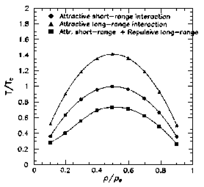
Figure 21: Phase diagrams for different types of interactions, see explanations in the text [235].

where $\epsilon=E/A$ is the energy per particle. $C_{V}$ shows a maximum for every value of $M$ at $T_{c}(M)$ which signals a continuous phase transition between two phases. The corresponding phase diagram is shown in Fig. 21. The analytic expression of $\mathcal{Z}$ allows for the determination of all thermodynamic quantities and the construction of the caloric curve $T=f(E)$ which is a monotonously increasing function. This is due to the fact that $C_{V}$ remains finite at the transition point for any value of $\rho/\rho_{0}$ [235]. Only the derivative of $C_{V}$ shows a discontinuity at the transition points.

The model can be extended to the case where particles interact through short or/and long range interactions

$$H=K - [V_{01}\!\!\sum_{<n.n>_{1}}\!\!s_{i}s_{j}+V_{02}\!\!\sum_{<n.n>_{2}}\!\!s_{i}s_{j}+\cdots+V_{0m}\!\!\sum_{<n.n>_{m}}\!\!s_{i}s_{j}]$$

$$+ \mu\sum_{i}s_{i}+\lambda\sum_{i}(2s_{i}-1)^{2}$$

where $K$ is the kinetic energy and $<n.n>_{k}$ has been defined below (32). A sensible parametrization in the case of nucleus would correspond to

$$V_{01} = V_{s}+V_{l}^{(1)}$$

$$V_{02} = V_{l}^{(2)}$$

$$\vdots$$

$$V_{0m} = V_{l}^{(m)}$$

where $V_{s}>0$ stands for the short range nuclear potential and $V_{l}^{(k)}<0$ for the long range repulsive Coulomb interaction parametrized in the following form

$$V_{l}^{(k)}=(Z_{p}/A)e^{2}/kd$$

where $Z_{p}$ is the total number of protons.

The partition function can be worked out in the framework of the spherical model in the same way as in the former case [235]. Fig. 21 shows typical phase diagrams for different cases involving long range interactions. As one can see, they lead to qualitatively similar results.

In the usual spherical model in which the constraint (35) is not implemented $\mu$ plays the role of a fixed magnetic field. Then, for $\mu\neq 0$, the magnetization can jump from $-M$ to $+M$ which corresponds to a first order transition. For $\mu=0$ the transition is continuous. This is not the case here since the magnetization $M$ (density $\rho$) is fixed, and not $\mu$ which is determined through (35). It explains why the transition is continuous in the present case for any value of $M$ or $(\rho/\rho_{0})$.

5.3.6 Thermodynamic properties of systems described by cellular models : numerical simulations

The former approach is a simplified even though quite realistic thermodynamic description of a disordered system. However, it does not allow to work out the fragment content of the system, which are accessible by means of numerical simulations [241]. This has been performed in the framework of the canonical ensemble for particles which experience short range nearest-neighbour interactions.

The Hamiltonian is written as

$$H=\sum_{i=1}^{A}\frac{p_{i}^{2}}{2m}s_{i}+\sum_{<i.j>_{1}}v_{12}(r_{ij})s_{i}s_{j}$$

where $v_{12}$ is the potential which acts between particles located in neighbour cells [228] at a distance $r_{ij}$ from each other, $A$ is the number of particles, $\rho=A/L^{3}$ the density of particles in a volume $V=L^{3}$ and the $s_{i}$’s are occupation numbers defined above. Periodic boundary conditions are imposed in the numerical simulations.

A Metropolis Monte Carlo procedure is used in order to generate events corresponding to different densities $\rho$ and temperatures $T$. For each $(\rho,T)$ the total number of events is $6\cdot 10^{4}$ and for each event about 5000 Metropolis iterations have been realized. Each iteration consists of either the move of a particle from its original cell to an empty cell, or its displacement inside a cell, or the determination of a new momentum. Each operation is realized with a probability $1/3$.

The latent heat is defined as

$$C_{V}=\frac{1}{A}\big{(}<U^{2}>-<U>^{2}\big{)}$$

where the average is an ensemble average and $U$ the potential energy of the system.

The calculations have also been extended to the microcanonical ensemble with fixed $A$ and energy $E$, by means of an algorithm described in ref. [242] which is well adapted to the present type of models. The probability for the existence of an event which has a configuration $s$ characterizing the positions and momenta of the particle is given by

$$W_{E}(s)\propto\big{(}E-U(s)\big{)}^{\frac{dV}{2}-1}\Theta\big{(}E-U(s)\big{)}$$

where $d$ is the space dimension, $V$ the volume and $\Theta$ the Heaviside function. Events are selected by means of a Metropolis procedure which accepts a configuration $s^{\prime}$ starting from a configuration $s$ with a probability

$$W_{s\to s^{\prime}}=\min\bigg{(}1,\frac{W_{E}(s^{\prime})}{W_{E}(s)}\bigg{)}$$

The temperature is obtained from

$$T=2<K>/Vd$$

where $<K>$ is the average kinetic energy of the particles.

Typical examples of the behaviour of $C_{V}$ and the caloric curve are shown in Fig. 22. The specific heat presents a more or less pronounced enhancement for some value of $T$. This enhancement is taken as the finite size restriction of a point which determines the phase separation line between a liquid and a gas in the thermodynamic limit. The numerical simulations show a smooth monotonous increase of the energy with temperature for fixed volume which is very similar to the results obtained in the framework of liquid gas models. For these small values of $A$ and $V$ it is not possible to identify the order of the transition. It is also remarkable to see that canonical and microcanonical calculations are very close to each other, even though the size of the system and the volume which contains it are small. We shall come back to this point and develop it in section 6.

The identification of bound clusters leads to the separation of the fragment content into two areas of the $(\rho,T)$ phase diagram separated by the equivalent of a Kertész line, above which the system contains essentially individual particles and small fragments, whereas large clusters are present below it. The separation line is expected to correspond to a power law fragment mass distribution in the limit of an infinite system. The presence of the power law behaviour is detected by analysing the calculated mass distributions.

The results are shown in the phase diagram of Fig. 23. Several remarks are in order. The thermodynamic separation line shows a dip at $\rho=0.5$. This is a finite size effect. A study of this point on a spin model which presents the same property confirms this point, see below in section 6. The separation line itself is not rigorously determined, there exists other means to fix it and furthermore it does not correspond to the limit of the infinite system. Contrary to the result of ref. [218], the Kertész line stays above the separation line for all values of $\rho$ but does not end at $\rho=0.5$. Furthermore, at $\rho=0.5$ the thermodynamic critical point does not coincide with the corresponding point on the Kertész line. The reasons for this are not easy to identify clearly. It makes sense to believe that all these points are related to finite size effects and possibly also the numerical precision with which the relevant quantities can be obtained. The determination of critical exponents by means of finite size scaling arguments has not been performed. The analysis and outcome would be similar to the ones obtained in the framework of another model which will be discussed below.

The remarkable point which may be retained from this study is the fact that the a priori more sophisticated cellular models discussed here are very close to the more schematic lattice gas models. If there are quantitative differences it is, at present, out of scope to judge which is quantitatively closer to the experiment.

6 Finite nuclei and phase transitions : present experimental and theoretical status

The experimental quest for a thermodynamic phase transition in nuclear matter received a new impetus in 1995 with the work of Pochodzalla et al. who tried to construct the so called caloric curve [243]. If nuclear matter would behave like a Fermi gas one would expect an increase of the temperature $T$ with excitation energy $E^{*}$ such that $T\propto E^{*1/2}$. Deviations could indicate the existence of a phase transition which, following classical arguments, is expected to be of the liquid-gas type.

However, nuclei are finite and the asymptotic limit of infinite matter is experimentally out of reach. The situation which is common to other fields like physics of aggregates and mesoscopic systems in condensed matter physics needs the development of new tools which may allow to detect the existence of the transition through the study of the behaviour of physical observables which characterize finite systems.

In the present section we try to give an overview of the recent experimental efforts which have been made and the theoretical investigations which have been initiated, specifically with the help of lattice-type models in order to detect a possible phase transition and unravel its nature in excited nuclear matter under the assumption that experimental measures are made on thermodynamically equilibrated systems.

6.1 Caloric curves and phase transitions : experimental status

The caloric curve which relates the internal energy of an excited system at thermodynamic equilibrium to its temperature is a priori the simplest experimental tool to look for the existence of a phase transition. The first determination attempted by the ALADIN collaboration [243] collected the outcome of ${}^{197}Au$ on ${}^{197}Au$ collisions at $600\,MeV\!\cdot\!A$ with data obtained by means of less energetic collisions. The excitation energy was determined by following the procedure prescribed in ref. [182] and the corresponding temperature fixed by means of arguments relating this quantity to the so called double ratio procedure [244], in the present case the ratios of ${}^{3}He/^{4}He$ and ${}^{6}Li/^{7}Li$ isotopes. The corresponding curve showed the features of a rather strong first order transition, with a characteristic close to constant temperature $T$ over a large energy interval lying between 3 and $10\,MeV$ excitation energy per nucleon, which may be interpreted as a sign for the generation of latent heat and followed by a strong increase of $T$ with excitation energy above $10\,MeV$. A critical discussion followed this observation, in which the hypotheses and simplifications underlying the definition of the temperature, the freeze-out density and the increase of $T$ at high excitation energy were examined [245].

A similar analysis by means of $1\,GeV\!\cdot\!A$ collisions of $C$ on $Au$ was initiated soon after this first attempt [246]. The reaction was interpreted as a two-step process, a prompt stage with the emission of light particles and a second step corresponding to the decay of an equilibrated system undergoing fragmentation. The outcome of the analysis lead to a smooth caloric curve from which any clear sign corresponding to a first order transition was seemingly absent, showing at most the possible existence of a continuous transition. In this experiment the temperature was determined in terms of two different isotope ratios, $(^{3}He/^{4}He)/(^{6}Li/^{7}Li)$ and $(^{3}He/^{4}He)/(d/t)$. The results were essentially confirmed later in a further experiment [247].

The INDRA collaboration considered $Ar$ on $Ni$ collisions at 52 and $92\,MeV\!\cdot\!A$ in order to investigate this point [248]. Several double isotopic yield ratios were used in order to define the temperature. They led to different slopes in the temperature increase as a function of the excitation energy. The issue of the experiment and its interpretation have been performed by means of statistical models [138, 139, 142]. A criticism has however been raised [249] which claims that the observation of the transition may have been missed because of the choice of too large steps in energy binnings.

At this stage the ALADIN collaboration considered the problem of the determination of the temperature by means of an analysis of $Au$ on $Au$ collisions at $1000\,MeV\!\cdot\!A$ [225] which was determined through different isotopic yield ratios and corrected for sequential evaporation from primary fragments. In this experiment, temperatures were also defined by means of excited state populations [250, 251]. Both types of temperatures are shown in Fig. 24. Those obtained from population yields are remarkably constant as a function of the excitation energy per particle, in contrast to the temperatures obtained by means of isotopic yield ratios. The interpretation of this apparent inconsistency leads to the conclusion that these temperatures may correspond to the final stage of fragment emission. The corrected new caloric curve emerging from the use of isotopic yields does no longer show a clear plateau-like behaviour. At the highest value of the excitation energy there remains however a sizable rise in the temperature which seems to indicate the entrance into a new phase.

A further attempt has been performed by bombarding $Ag$ and $Au$ with $4.8\,GeV\ ^{3}He$ ions [252]. The temperature was fixed by means of the double ratio yield $(^{2}H/^{3}H)/(^{3}He/^{4}He)$. A slope discontinuity is observed for $E^{*}/A\simeq 2-3\,MeV$ which is followed, with increasing excitation energy, by a monotonic rise up to the measured energy $E^{*}/A\simeq 10\,MeV$. The curve is in qualitative agreement with the theoretical predictions of the Expanding-Evaporating Source model (EES) [92, 253] and the Statistical Multifragmentation Model (SMM) [110, 254].

More recently, a further result has been obtained on excited systems with $A\simeq 110$ particles produced by means of different projectiles and targets with a bombarding energy of $47\,MeV\!\cdot\!A$ [255]. The temperature was obtained from the double ratios $(d/t)/(^{3}He/^{4}He)$. An analysis based on coalescence models [256, 257, 258, 140, 259] was used in order to follow the evolution of temperature and densities. Calorimetry measurements fix the excitation energies. The experimental points combined with former results [260] show a steep increase of $T$ up to $E^{*}/A\simeq 3.5\,MeV$. The temperature stabilizes for $3.5\leq E^{*}/A\leq 7\,MeV$ around $T\sim 7\,MeV$.

The analysis and comparison of results obtained by different groups show hardly more than qualitative similarities and are rather non conclusive as far as the existence and possible order of a phase transition are concerned. They are plagued by different problems which are not only related to finite size effects or the equilibration problem, but also by the fact that in the experiment the system undergoes expansion, sequential decay of primary excited fragments, apparently temperature determinations can lead to inconsistent results. These problems have been investigated by several groups [261, 262, 263, 264, 265, 266, 267]. Further new methods for the determination of the temperature have been proposed [268]. As the matter stands, there are signs which point towards the existence of a transition. The caloric curve may however not be the most adequate tool to confirm it. We shall discuss this point in the next section.

6.2 Signs for phase transitions in finite systems : tests and applications to the nuclear case by means of lattice models

Nuclei are finite systems, hence experimental observations refer to small systems, far from the thermodynamic limit. Contrary to other aggregates or quantum dots whose size can be experimentally varied and controlled, there is no such flexibility in fixing the number of constituents over large scales here. It shows that even if the experimental determination of physical observables could be fully tested, there would remain the problem of the small size limit. This point raises the question of the detection of the existence and nature of a phase transition through the measurements on finite systems. The signs for the existence of transitions clearly exist, they are seen in finite systems since infinite systems do not exist, and one may speak about phase transitions in finite systems [270]. The determination of their order necessitates good tests and a great deal of caution. This point has been raised in several fields of physics in the recent past. We review some of the methods and tests which have been proposed in the next section before applying them to lattice models and the analysis of experimental data.

6.2.1 Tests for the existence of phase transitions from finite system analysis

There exist several characteristic properties which may signal that a finite system can show a critical behaviour related to a phase transition.

Close to a critical point observables follow scaling laws which relate their behaviour at different scales, i.e. for different sizes of the system. They allow for the determination of critical exponents which characterize the singular behaviour at the critical point in the limit of an infinite system. This property has already been presented and discussed in subsection 4.3 above [197]. We shall come back to it below.

A second characteristic of finite systems which are close to a phase transition is the enhancement and universal behaviour of fluctuations in observables and order parameters. This type of properties is commonly studied [271] and has been used [272] as will be shown below. Recently the properties of order parameters of finite systems close to a second order transition have been studied in the framework of a finite size scaling approach [273]. It comes out that order parameters can be characterized by probability densities which possess specific properties depending on their location with respect to the critical point. In particular, at the critical point, they show universal scaling and deviations from a gaussian behaviour in the tails. This behaviour is valid for both equilibrium as well as off-equilibrium processes in systems which undergo second order transitions. The method could work as an alternative to the determination of critical exponents. Applications will certainly be developed in the near future.

Informations about the thermodynamic properties of small extensive and non-extensive systems (for which the sum of the energies and entropies is not the sum of energies and entropies of their parts, f.i. if long range interactions are present) can be very efficiently analysed in the framework of the microcanonical ensemble. This aspect has been extensively discussed, see f.i. [270] and refs. therein. The important point of practical importance concerns the topology of the entropy $S(E,A)$ of a system with $A$ particles and total energy $E$ [270]. In the presence of a first order transition, the entropy shows convexity (negative curvature) in certain ranges of energy. This behaviour is specific to the microcanonical ensemble which is able to give a faithful description of inhomogeneous systems. In the caloric curve the temperature is a multivalued function of the energy, showing a bend (“$S$” curve) and, as a consequence, the specific heat can get negative over some intervals of energy. The physical explanation for this phenomenon is the existence of a surface tension which is generated by the coexistence of two phases. Indeed, the creation of intra-phase surfaces generates an entropy loss $\Delta S_{Surf}$ which can be obtained from the relation [274]

$$\Delta S_{Surf}=\frac{\gamma}{T_{c}}\cdot\frac{\Sigma}{A}$$

where $\gamma$ is the surface tension, $T_{c}$ the transition temperature, $\Sigma$ the surface area of all species with mass larger than $1$, and $A$ the number of particles. This remarkable property shown by finite systems will be used below as a main tool in order to detect and characterize the behaviour of fragmenting nuclear systems.

The present collection of tests is certainly not exhaustive, there may exist other means to detect signs for phase transitions. One of them which grounds on the Yang and Lee theory has already been mentioned in section 5.1.3 [199]. Recently Ma [275, 276] proposed to use the enhancement of entropy production at the pseudo-transition point and claimed that Zipf’s law [277] is verified at the transition point. This has been tested numerically by means of calculations involving an LGM model and Molecular Dynamics simulations. Ref. [278] discusses the correlation between an “$S$” curve in the caloric curve in the microcanonical framework, the thermodynamic temperature $T=(\partial E/\partial S)_{V}$ and the temperature determined from the kinetic energies of the constituents of the system. It is shown that the caloric curve obtained by means of the thermodynamic temperature shows a bend if this is the case for the kinetic temperature, but that the reverse is not true.

6.2.2 Applications of the tests to models of nuclear fragmentation. Finite size scaling and microcanonical description

The finite size scaling test for the determination of the order of a phase transition by means of the determination of critical exponents has been recently applied to a lattice model, the Ising Model with Fixed Magnetization (IMFM) [197]. Its canonical partition function reads

$$\mathcal{Z}_{V}=\sum_{[\sigma]}\exp\big{(}\beta V_{0}\!\sum_{<n\cdot n>_{1}}\!\sigma_{i}\sigma_{j}\big{)}\ \delta_{M,\widehat{M}}$$

where $V_{0}$ is a negative potential strength, $M=2\rho/\rho_{0}-1$ the “magnetization” related to the relative density $\rho/\rho_{0}$, $\widehat{M}$ a fixed value of $M$, $\{\sigma_{i}=\pm 1\}$ related to the lattice site occupations $\{s_{i}=0,1\}$ in the notation of subsection 5.3.5.

The model is equivalent to an LGM except for the fact that the number of particles, $A=\sum_{i}s_{i}$, is strictly fixed and, as a consequence, $\rho/\rho_{0}$ is fixed if the volume $V$ is fixed. It is a non trivial model whose properties have been investigated recently [279]. In the canonical ensemble the kinetic energy plays a trivial role, therefore there is no need to introduce it if one looks for critical properties of the system in this framework.

The system governed by the IMFM shows a phase transition with a phase diagram $(\rho,T)$ which has the same topology as LGM and related models, see f.i. Fig. 16. However in the ordinary Ising model with zero magnetic field contribution, the magnetization jumps when the system enters the coexistence phase at $T<T_{c}$. Since the present description keeps the magnetization fixed, the order of the transition is a priori not clear.

The problem has been investigated numerically, first in the canonical framework for a system with fixed volume. The sensible quantity which has been worked out is the specific heat

$$C_{V}=3V(<E^{2}>-<E>^{2})$$

where $V$ is the volume and $E$ the energy of the system. At the separation line, one looks for the asymptotic behaviour of $C_{V}$ in the form

$$C_{V}\propto(\beta-\beta_{c}^{Th})^{-\alpha}$$

$\beta^{Th}=T^{-1}$, $\beta_{c}^{Th}=(T_{c}^{Th})^{-1}$, $T_{c}^{Th}$ being the thermodynamic transition temperature of the infinite system for fixed density $\rho$ and $\alpha$ a real positive exponent which may help to characterize the universality class to which the transition belongs.

Using finite size scaling arguments and writing

$$C_{V}(L) = A+BL^{\alpha/\nu}$$ (38)

$$\beta_{c}(L)-\beta_{c}(\infty) = \bar{A}L^{-1/\nu}$$

where $A,B,\bar{A}$ are real constants and $L$ is the linear size of the system, it is possible to obtain $\nu$ and $\alpha/\nu$, hence $\alpha$, corresponding to the thermodynamic limit [197]. Typical results for the evolution of $C_{V}$ with the size of the system by identification of the maximum of this quantity for fixed $\rho$ are shown in Fig. 25 for two values of $\rho/\rho_{0}=(\widehat{M}+1)/2$. In this figure $\alpha/\nu$ is read from the slope of the curves which should behave like rigorously straight lines if the scaling hypothesis (38) is working. The straight line behaviour is observed for $L$ large enough $(L\geq 28)$, although there are deviations at close inspection. The values of $\nu$ and $\alpha$ for $\rho/\rho_{0}=0.3$ and 0.5 could be compatible with the universality class of the Ising model although this is not absolutely established since the behaviour for $L=48$ could still be transitory. This value of $L$ in $3d$ space requires already a large numerical effort.

The non completely conclusive situation led to further investigations [280]. First, the topology of the system on the critical line is very similar for different values of the density, showing a quite homogeneous pattern. Second, the evolution of the caloric curve shows a change of slope which gets more accentuated with increasing size of the system, with the presence of an inflexion point which is characteristic of a continuous transition.

A sharper test consists of the use of the microcanonical ensemble. Here the kinetic energy part is taken into account and the procedure is described in subsection 5.3.6. As discussed above, a first order transition should manifest itself by a temperature which is a multivaluated function of energy, and this is not the case if the transition is continuous. This phenomenon was numerically checked on the Potts model which can effectively be of first or second order for different numbers of spin directions on a given site [160, 281]. The application of the microcanonical algorithm to the IMFM does not show the expected “$S$” curve as it would be the case for a first order transition, see Fig. 26. This fact does however not lead to a definite answer because it is expected that for a fixed volume the caloric curve in the infinite system never shows a plateau in the presence of a first order liquid-gas type phase transition but only a more or less steep change of slope, the plateau arises for fixed pressure as recalled in ref. [282]. Furthermore, as already mentioned, the finite system announces a transition which may not necessarily be the one which is really observed in the thermodynamic limit.

Two conclusions can be drawn from this study. First, the present model deals with two constraints, fixed volume and fixed number of particles. These constraints may play a critical role in finite systems. This can be seen on the Potts model. For $q\geq 5$ where $q$ is the number of spin directions on a site, the caloric curve should show an “$S$” curve. When constraints are applied on the spin population of different spin directions at the different sites of the system the bend disappears [280].

The importance of constraints has of course also consequences for the interpretation of experimental results which depend of the physical conditions under which data are collected. Fixed volume is an illustration of the effect of constraints.

6.2.3 Fluctuations and criticality

As already seen above [273], critical phenomena are strongly correlated with large fluctuations in the thermodynamic variables. This property has been exploited recently by Chomaz and Gulminelli [272, 283, 284] in the framework of the microcanonical ensemble. These authors have explicitly shown on a simple model how the specific heat which can be defined in terms of energy fluctuations can reach negative values.

A closed system with energy $E_{t}$ is divided into two subsystems, 1 and 2, with energy $E_{1}$ and $E_{2}$, $E_{t}=E_{1}+E_{2}$. Then the energy distribution in subsystem 1 can be written as

$$P_{1}^{E_{t}}(E_{1}) = \frac{W_{1}(E_{1})W_{2}(E_{t}-E_{1})}{W(E_{t})}$$ (39)

$$= \mathcal{N}\exp[S_{1}(E_{1})+S_{2}(E_{t}-E_{1})-S(E_{t})]$$

where $\mathcal{N}$ is a normalization factor, $W_{i}(E_{i})$ is the density of states of the system $i$ at the energy $E_{i}$ and $S_{i}(E_{i})$ its entropy. $W(E_{t})$ is a convolution of partial densities

$$W(E_{t})=\int_{0}^{E_{T}}\mathrm{d}E_{1}\exp[S_{1}(E_{1})+S_{2}(E_{t}-E_{1})]$$

At equilibrium $W(E_{t})$ is maximum for

$$\frac{\partial S_{1}}{\partial E_{1}}\bigg{|}_{\overline{E}_{1}}=\frac{\partial S_{2}}{\partial E_{2}}\bigg{|}_{E_{t}-\overline{E}_{1}}$$ (40)

where $\overline{E}_{1}$ corresponds to the stationary point where the equality is realized. Relation (40) shows that the temperatures $T_{1}$ and $T_{2}$ are the same in both subsystems, $T_{1}=T_{2}=\overline{T}$ as expected for a system in thermodynamic equilibrium.

Close to the maximum of $W(E_{t})$ it is reasonable to parametrize $P_{1}^{E_{t}}$ by a gaussian

$$P_{1}^{E_{t}}(E_{1})=(2\pi\sigma_{1}^{2})^{-1/2}\exp[-(E_{1}-\overline{E}_{1})^{2}/2\sigma_{1}^{2}]$$ (41)

Then

$$\frac{\partial^{2}P_{1}^{E_{t}}(E_{1})}{\partial E_{1}^{2}}\bigg{|}_{\overline{E}_{1}}=-(2\pi)^{-1/2}\sigma_{1}^{-3}$$ (42)

From (39), for $\mathcal{N}=(2\pi\sigma_{1}^{2})^{-1/2}$

$$\frac{\partial^{2}P_{1}^{E_{t}}}{\partial E_{1}^{2}}\bigg{|}_{\overline{E}_{1}} = -\frac{1}{\overline{T}^{2}}\Bigg{(}\frac{C_{1}+C_{2}}{C_{1}C_{2}}\Bigg{)}$$ (43)

$$\textrm{where}\quad C_{i} = -\frac{1}{T_{i}^{2}}\Bigg{(}\frac{\partial^{2}S_{i}}{\partial E_{i}^{2}}\Bigg{)}^{-1}=\frac{\mathrm{d}\overline{E}_{i}}{\mathrm{d}E_{t}}$$

is the specific heat of the system $i$. Equating (42) and (43) and introducing

$$\overline{C}=C_{1}+C_{2}$$ (44)

leads to

$$\overline{C}=\frac{C_{1}^{2}}{C_{1}-\sigma_{1}^{2}/\overline{T}^{2}}$$

If now subsystem 1 corresponds to the kinetic energy part of the system with energy $E_{k}$ and specific heat $C_{k}$ and subsystem 2 to the potential contribution $E_{p}$ then

$$\overline{C}=\frac{C_{k}^{2}}{C_{k}-\sigma_{k}^{2}/\overline{T}^{2}}$$ (45)

where $C_{k}=\frac{3}{2}A$ and $A$ is the number of particles. The knowledge of the temperature $\overline{T}$ of the system and the kinetic energy fluctuations characterized by $\sigma_{k}^{2}$ allow then to determine the heat capacity of the system in the framework of the microcanonical ensemble. It is clear that if $\sigma_{k}^{2}$ gets larger than $C_{k}\overline{T}^{2}$, $\overline{C}$ gets negative which corresponds to an “$S$” bend in the caloric curve. The analysis requires however some care. There is a priori no justification for the distribution (41) to be gaussian nor for (44) to be strictly true in the vicinity of a critical point. The lack of concavity of the entropy is the sign for it. There are however signs that, even if (44) is not strictly correct, the variance of the real distribution can be assimilated to the variance of a gaussian distribution if the number of particles is not too small [285]. The correction to the heat capacity due to higher moment contributions to (42) has been discussed in ref. [272]. The kinetic energy distribution is in principle experimentally accessible.

The relation (44) has been applied to lattice models of the same type as the one whose Hamiltonian is used in subsection 5.2.2 [284]. The partition function reads

$$\mathcal{Z}_{\lambda}(E)=\sum_{V}W_{V}(E)e^{-\lambda V}$$

where $W_{V}(E)$ is the density of states at energy $E$. The volume of the system is not fixed here but fluctuates. This is described by means of the introduction of a Lagrange multiplier $\lambda$ which is interpreted as a quantity proportional to a pressure $P=\lambda T_{\lambda}$ where $T_{\lambda}=\partial\ln\mathcal{Z}_{\lambda}/\partial E$.

The equation of state for this model has been studied numerically in the 3-dimensional space $(T,E,\lambda)$. One observes a backbending effect if one represents $P=\lambda T$ as a function of the average volume $<V>$ which is interpreted here as being the consequence of mass and energy conservation constraints. An “$S$” bend appears also in the caloric curve on the $(E,T)$ surface. For strictly fixed volume the caloric curve does not show any backbending. This is illustrated in Fig. 27 in which the specific heat is represented as a function of energy using (45). With this interpretation the puzzle concerning the order of the transition which was discussed in subsection 6.2.2 [280] is apparently explained, the shape of the caloric curve depends on the thermodynamic variables which are considered [282]. This message is of some importance in the framework of experimental analyses.

6.3 Experimental construction of the caloric curve and determination of the specific heat

Different attempts have been made since the pioneering work already mentioned above [ALADIN, INDRA, EOS,…] in order to construct the caloric curve starting from experimental data.

The reaction ${}^{28}Si$ on ${}^{100}Mo$ leading to an incomplete fused system has been used in order to relate the excitation energy per particle $e^{*}$ of the system to a so called apparent temperature $T_{app}$ which is obtained from the slopes of the energy distributions of emitted light particles [286].

$$\frac{\mathrm{d}\sigma}{\mathrm{d}E_{kin}}\propto(E_{kin}-B)\,\exp\Bigg{[}-\frac{(E_{kin}-B)}{T_{app}}\Bigg{]}$$

where $E_{kin}$ is the kinetic energy and $B$ the Coulomb barrier. $T_{app}$ which is not the thermodynamic temperature $T_{th}$ is shown to be a sensible quantity, both $T_{app}$ and $T_{th}$ show the same trend as a function of the energy. The outcome of the experience is in reasonable agreement with calculations performed in the framework of the MMMC model. Since this model indicates the existence of a phase transition, it is tempting to conclude that it is also experimentally true since model calculations and experimental data have been worked out under the same physical conditions. It should nevertheless be mentioned that the results do not constitute a full proof because there remain some differences between the calculations and the data analysis. Former data from the Texas A & M-group [260] are in agreement with those discussed here.

The problem concerning the determination of the temperature has also been raised in the framework of a sequential decay model in which fragmentation evolves in time by means of successive binary break-ups of excited fragments [287] in a way which is similar to the approach of ref. [94]. The analysis [142, 288] of different definitions of the temperature leads to different results, due to the time-dependence of the process. It comes out that the experimental caloric curve [243] can be reproduced over a large range of excitation energies.

Very recently an attempt to detect the signal of a phase transition through the determination of the specific heat has been made by the Multics-Miniball collaboration at the cyclotron of the Michigan State University [289, 290]. The excited system has been generated by means of $Au$ on $Au$ collisions at $35\,MeV\!\cdot\!A$. The angular distributions of fragments show isotropy which is a sign for possible equilibration [289]. The conditions are such that the number of involved particles and the total energy are fixed, so that the arguments which characterize microcanonical ensembles can be applied. The correlation between the excitation energy $E^{*}$ and the temperature is fixed through the balance in energy at the freeze out

$$m_{0}+E^{*}=\sum_{i=1}^{M}(m_{i}+E_{i}^{int})+E_{Clb}+\frac{3}{2}(M-1)T$$

where $m_{0}$ is the initial mass excess, $m_{i}$ the mass excesses of the fragments, $E^{*}$ the excitation energy of the source, $E_{i}^{int}$ the internal excitation energy of fragment $i$, $E_{Clb}$ the Coulomb repulsion energy, $M$ the multiplicity and $T$ the temperature which is fixed by the balance equation. No collective energy is taken into account. A backtracing procedure is used in order to correlate the asymptotically observed events to the freeze-out configurations. The comparison of $E^{*}(T)$ with SMM predictions are in good though not perfect agreement. The heat capacity shows a sizable enhancement for temperatures lying between 4 and $6\,MeV$.

In a further step the experiment has been analysed following the microcanonical prescriptions of Chomaz and Gulminelli, see subsection 6.2.3 [283, 284]. The total energy $E_{t}$ has been decomposed into a kinetic and a potential contribution

$$E_{t}=m_{0}+E^{*}=E_{1}+E_{pot}$$

$$\textrm{where}\quad E_{pot}=\sum_{i=1}^{M}m_{i}+E_{Clb}$$

and $E_{Clb}$ is the Coulomb energy acting between the fragments at freeze-out. This energy has been evaluated by means of simulations in which primary fragments are randomly distributed in a freeze-out volume equal to three times the normal volume. Two extreme hypotheses have been used. Either (1) all charged species including all light particles were considered as primary or (2) the totality of neutrons and light particles was distributed over the final fragments. These choices correspond to the procedures used in the framework of the SMM and MMMC models. In this way, one fixes the ensemble averaged quantities over sets of events $<E_{1}>,\ <E_{1}^{2}>,\ \sigma_{1}^{2}$ and $C_{1}=\frac{3}{2}<(M-1)>$ where

$$<E_{1}>=\Big{<}\sum_{i=1}^{M}a_{i}\Big{>}\,T^{2}+\Big{<}\frac{3}{2}(M-1)\Big{>}\,T$$

and $a_{i}$ is the level density of fragments $i$.

The results corresponding to cases (1) and (2) are shown in Fig. 28. In both cases one observes the signs for a divergent behaviour of the heat capacity at two values of the energy and the expected negative contributions to the specific heat in the microcanonical framework. The stability of this result with respect to variations in the size of excitation energy bins, the assumptions on $E^{*},\,E_{t}$ and the choice of the $a_{i}$’s have been checked.

The same type of analysis has been performed with the INDRA detector on the outcome of the reaction $Xe$ on $Sn$ at 32 and $50\,MeV\!\cdot\!A$ central collisions [147, 291]. In order to extract the kinetic energy fluctuations which enter the determination of the specific heat, it has been necessary to substract the collective effects which are present and to take care of the particle emission which takes place during the expansion phase of the process. One of the two divergences which develop in the heat capacity is observed as well as the onset of negative values for this quantity. The second singularity is not seen because the excitation range does not cover the whole interval of energy corresponding to the coexistence of the phases.

7 Summary and conclusions

In the present report we tried to summarize the present knowledge about the properties of excited nuclear matter which can be gained through the confrontation of simple classical models describing finite systems and experimental facts obtained from energetic collisions between finite nuclei.

As an introduction we developed in section 2 some historical facts concerning the beginning of the activities in the field of nuclear fragmentation, both on the side of the experiment with the observation of power laws in the fragment size distributions, the introduction of the droplet model and the theoretical developments based on mean field approaches to nuclear matter and microscopic transport descriptions in the mean field approximation and beyond.

We recalled that there are two main difficulties in the interpretation of experimental data obtained by means of energetic nuclear collisions. The first concerns the finite size of nuclei and the second the fact that the colliding objects evolve with time, from an initial compact system to an expanded system at the nuclear freeze-out where the nuclear interaction between fragments does no longer act, and finally to the asymptotic stage where the remnants of the reaction are identified by detectors. The second point leads to the question of the setting up of chemical and thermodynamic equilibrium. At lower energies there are signs which show that nuclear systems are able to absorb and spread sizable amounts of energy more or less uniformely over phase space.

Thermodynamic equilibration is discussed in section 3 in which some of the efforts which have been made in order to get information about this point are developed. For the moment, equilibration seems to be a sensible concept since experimental results can be consistently interpreted in this framework, even though no strong and clear-cut proof for it exists up tp now.

One of the first and more spectacular successes in the field concerns the multiplicities of fragments of different sizes which are amazingly well reproduced by means of simple minded percolation models. This point is presented and discussed at length in section 4. Universality properties are clearly identified and the intriguing power law behaviour which was observed and was of central interest in the early days appears again in a new context. Since percolation concepts are minimal information concepts it may appear that there is not much information to be gained from observables like fragment size distributions. The reasons for this may be related to the fact that highly excited nuclei behave like disordered systems, and as it is the case for many other systems of this type in other fields of physics, the details of their dynamical properties are of very restricted importance. Universality properties of physical systems are remarkable because they work as a link between objects and phenomena which are seemingly very different from each other and at the same time are insensitive to the detailed information about the system.

The success of percolation drew the attention towards other simple classical models which have a strong kinship with percolation but are defined in terms of Hamiltonians. Some of them, so called lattice and cellular models, are described and analysed in section 5. Their simplicity and at the same time their universal character leads to the observation that they work as good tools for the investigation of the properties of fragmenting nuclei. Most of them are able to reproduce the properties related to fragment multiplicities. They show very useful for the investigations of effects related to finiteness in search for and analysis of phase transitions. They predict the possible existence of two types of transitions which are not necessarily correlated in an evident way, a thermodynamic transition and a continuous percolation type transition which for systems with a density between nuclear density and half nuclear density occurs at temperatures which are higher than those which correspond to the thermodynamic transition. This point is not yet clearly understood, although it does not lead, a priori, to any contradiction. It opens up the old question concerning the link with Fisher’s droplet model. Numerical simulations on different models lead to very similar thermodynamic properties.

The final part, section 6, deals more specifically with the problem of the existence and characterization of phase transitions and signs which show their existence in finite systems. For such types of analyses specific tools are needed. Some of them have been proposed very recently, at a time where similar considerations are developed in other fields of physics dealing with small systems. Some of these tools are explicitly described. Theoretical methods relying on a microcanonical description and aimed to detect transitions which have been developed in the framework of lattice models have been presented. Their application in the analysis of experimental data is described at the end of the section.

A great wealth of information has been accumulated about the characteristics and behaviour of highly excited nuclei, their fragmentation properties and the existence of a genuine phase transition of a type which may be similar to the classical liquid-gas transition. The last point remains however to be confirmed. Many pieces of the puzzle have been brought together, however the whole picture is not yet totally clear. Experimental confirmation of the transition has to be brought, scaling properties further investigated, the question of the possible coexistence of two types of transitions elucidated. Quantum mechanical aspects which have been quoted and the importance of quantum effects have to be further worked out and analysed. Last, there remains the difficult problem of the possible off-equilibrium character of the fragmentation process of a finite critical system. The study of critical off-equilibrium dynamics is a relatively recent field of research, still in its infancy. It is a field to which the nuclear physics community interested in the behaviour of highly excited and decaying systems of particles could certainly bring its contribution.

FIGURES

Figure 7: Plot of the $(a,s)$ plane where the degeneracy $g(a,s)$ is non zero. For fixed $A$ $(=A_{1}$ or $A_{2})$ only the hatched areas contribute to the mass spectrum [168].

Figure 8: Mass yields obtained with the parametrization of the bond probability $p(b)$ given in the text for (a) $p+Ag$ at $11.5\,GeV$, $p_{0}=0.65$; (b) $p+Ta$ at $5.7\,GeV$, $p_{0}=0.69$; (c) $p+^{197}Au$ at $11.5\,GeV$, $p_{0}=0.70$ [171].

Figure 9: $\ln S_{3}$ as a function of $\ln S_{2}$ for single events. Part (a) corresponds to the break-up of gold nuclei, part (b) to a cubic bond simulation with 216 sites and bond probabilities $0<p<1$, [174].

Figure 10: The quantity $\gamma_{2}$ defined in (22). The upper part corresponds to the fragmentation of gold and the lower part to percolation simulations, [175].

Figure 11: Size of the largest fragment for different events as a function of $S_{2}$. (a) Experimental results obtained from 376 events. (b) Bond percolation results in a cubic volume with 216 sites, 4000 realizations [174].

Figure 18: Comparison of percolation results (upper part) with A2 algorithm (lower part). [224].

Figure 22: Caloric curve and specific heat for a finite size system, $L=8^{3}$, and density $\rho/\rho_{0}=0.5$. Canonical and microcanonical simulations coincide [241].

Figure 23: The phase diagram obtained with the cellular model described in the text [241]. See discusion in the text.

Figure 24: Isotope temperature $T_{HeLi}$ (full triangles) and temperatures obtained by means of excited state population rate measurements (open symbols) as a function of the excitation energy per nucleon for ${}^{197}Au$ on ${}^{197}Au$ at $E=1000\,MeV\!\cdot\!A$ [225].

Figure 25: Fit of $C_{V}^{max}$ as a function of the linear size $L$ of the system for different densities. Crosses indicate different sizes. The largest size is $L=48$ [197].

Figure 26: Caloric curve calculated for a 3D IMFM for a system of linear size $L=10$, $\rho/\rho_{0}=0.3$ (upper part), $\rho/\rho_{0}=0.5$ (lower part). Canonical and microcanonical calculations are indistinguishable. See comments in the text [280].

Figure 27: Caloric curve, specific heat and kinetic energy fluctuations at constant pressure (left part) and constant volume (right part) calculated in the framework of the microcanonical ensemble [284]. See comments in the text.

Figure 28: Experimental heat capacities for the two extreme hypotheses which where made in order to evaluate $E_{Clb}$ (see text). The dotted curve corresponds to the Fermi-gas calculation [290].

References

- [1] A. Bohr and B.R. Mottelson, Nuclear Structure, World Scientific, 1998.
- [2] P. Ring and P. Schuck, The Nuclear Many-Body Problem, Springer-Verlag, 1980.
- [3] W. Greiner and J.A. Maruhn, Nuclear Models, Springer-Verlag, 1996.
- [4] M.L. Mehta, Random Matrices and the Statistical Theory of Energy Levels, Academic Press, New York, 1991.
- [5] Th. Guhr, A. Müller-Groeling and H.A. Weidenmüller, Phys. Rep. 299 (1998) 189 and refs. therein.
- [6] N. Bohr, Nature 137 (1936) 344.
- [7] L.D. Landau, JETP 30 (1956) 1058.
- [8] A.A. Abrikosov, L.P. Gorkov and I.E. Dzyaloshinskii, JETP 36 (1959) 900.
- [9] P. Nozières, Theory of Interacting Fermi Systems, W.A. Benjamin, Inc., New York, 1964.
- [10] A.B. Migdal, Nucl. Phys. 30 (1962) 239.
- [11] M. Lacombe et al., Phys. Rev. C21 (1980) 861.
- [12] R.B. Wiringa, V.G.I. Stoks and R. Schiavilla, Phys. Rev. C51 (1995) 38.
- [13] V.G.I. Stoks, R.A.M. Klomp, C.P.F. Terheggen and J.J. de Swart, Phys. Rev. C49 (1994) 2950.
- [14] R. Machleidt, F. Sammarruca and Y. Song, Phys. Rev. C53 (1996) R1483.
- [15] L. Engvik et al., Nucl. Phys. A627 (1997) 85.
- [16] S. Kahana, H.C. Lee and C.K. Scott, Phys. Rev. 180 (1969) 956.
- [17] B.A. Brown and B.H. Wildenthal, Ann. Rev. Nucl. Part. Sci. 38 (1988) 29.
- [18] R.W. Minich, S. Agarwal, A. Bujak, J. Chuang, J.E. Finn, L.J. Gutay, A.S. Hirsch, N.T. Porile, R.P. Scharenberg, B.C. Stringfellow and F. Turkot, Phys. Lett. B118 (1982) 458.
- [19] M.E. Fisher, Physics 3 (1967) 255.
- [20] H. Jaqaman, A.Z. Mekjian and L. Zamick, Phys. Rev. C27 (1983) 2782.
- [21] A.D. Panagiotou, M.W. Curtin, H. Toki, D.K. Scott and P.J. Siemens, Phys. Rev. Lett. 52 (1984) 496.
- [22] A.D. Panagiotou, M.W. Curtin and D.K. Scott, Phys. Rev. C31 (1985) 55.
- [23] Ph. Quentin and H. Flocard, Ann. Rev. Nucl. Part. Sci. 28 (1978) 523.
- [24] A.L. Fetter and J.D. Walecka, Quantum Theory of Many-Particle Systems, McGraw-Hill, New York, 1971.
- [25] G. Sauer, H. Chandra and U. Mosel, Nucl. Phys. A264 (1976) 221.
- [26] M.W. Curtin, H. Toki and D.K. Scott, Phys. Lett. B123 (1983) 289.
- [27] H. Schulz, L. Münchow, G. Röpke and M. Schmidt, Phys. Lett. B119 (1982) 12.
- [28] P. Bonche, S. Levit and D. Vautherin, Nucl. Phys. A427 (1984) 278.
- [29] P. Bonche, S. Levit and D. Vautherin, Nucl. Phys. A436 (1985) 265.
- [30] S. Levit and P. Bonche, Nucl. Phys. A437 (1985) 426.
- [31] H.R. Jaqaman, Phys. Rev. C39 (1989) 169.
- [32] H.R. Jaqaman, Phys. Rev. C40 (1989) 1677.
- [33] R.G. Newton, Scattering Theory of Waves and Particles, Springer-Verlag, 1982.
- [34] T.Y. Wu and T. Ohmura, Quantum Theory of Scattering, Prentice-Hall Series In Physics, 1962.
- [35] H.A. Weidenmüller, Prog. Part. and Nucl. Phys., Volume 3 (1980) 49.
- [36] P. Fröbrich and I.I. Gontchar, Phys. Rep. 292 (1998) 131.
- [37] A. Bonasera, F. Gulminelli and J. Molitoris, Phys. Rep. 243 (1994) 1.
- [38] J. Cugnon, A. Lejeune and P. Grangé, Phys. Rev. C35 (1987) 861.
- [39] A. Bonasera, M. Colonna, M. Di Toro, F. Gulminelli and H.H. Wolter, Phys. Lett. B244 (1990) 169.
- [40] M. Colonna, P. Roussel-Chomaz, N. Colonna, M. Di Toro, L.G. Moretto and G.J. Wozniak, Phys. Lett. B283 (1992) 180.
- [41] A. Bonasera, M. Colonna, M. Di Toro, F. Gulminelli and A. Smerzi, Nucl. Phys. A572 (1994) 171.
- [42] M. Colonna, Ph. Chomaz and J. Randrup, Nucl. Phys. A567 (1994) 637.
- [43] Ph. Chomaz, M. Colonna, A. Guarnera and J. Randrup, Phys. Rev. Lett. 73 (1994) 3512.
- [44] B. Jacquot, A. Guarnera, Ph. Chomaz and M. Colonna, Phys. Rev. C54 (1996) 3025.
- [45] B. Jacquot, A. Guarnera, Ph. Chomaz and M. Colonna, Phys. Lett. B386 (1996) 23.
- [46] M. Colonna, Ph. Chomaz and A. Guarnera, Nucl. Phys. A613 (1997) 165.
- [47] M. Colonna et al., Nucl. Phys. A642 (1998) 449.
- [48] M. Colonna, Ph. Chomaz, A. Guarnera and B. Jacquot, Phys. Rev. C51 (1995) 2671.
- [49] S. Ayik, M. Colonna and Ph. Chomaz, Phys. Lett. B353 (1995) 417.
- [50] V. Baran, M. Colonna, M. Di Toro and A.B. Larionov, Nucl. Phys. A632 (1998) 287.
- [51] M.F. Rivet et al., Phys. Lett. B430 (1998) 217.
- [52] D. Lacroix and Ph. Chomaz, Nucl. Phys. A636 (1998) 85.
- [53] W. Wen, P. Chau Huu-Tai, D. Lacroix, Ph. Chomaz and S. Ayik, Nucl. Phys. A637 (1998) 15.
- [54] J. Aichelin, Phys. Rep. 202 (1991) 233 and refs. therein.
- [55] A. Bonasera, M. Bruno, C.O. Dorso and P.F. Mastinu, “Critical Phenomena in Nuclear Fragmentation”, La Rivista del Nuovo Cimento 23 (2000) 1.
- [56] H. Feldmeier, Nucl. Phys. A515 (1990) 147.
- [57] H. Feldmeier and J. Schnack, Prog. Part. Nucl. Phys. 39 (1997) 393.
- [58] H. Feldmeier and J. Schnack, to be published in Rev. Mod. Phys. (July 2000), The American Physical Society.
- [59] H. Horiuchi, Nucl. Phys. A522 (1991) 257c.
- [60] A. Ono, H. Horiuchi, T. Maruyama and A. Onishi, Prog. Th. Phys. 87 (1992) 1185.
- [61] Y. Sugawa and H. Horiuchi, Phys. Rev. C60 (1999) 064607.
- [62] Y. Tosaka, A. Ono and H. Horiuchi, Phys. Rev. C60 (1999) 064613.
- [63] V. Latora, M. Belkacem and A. Bonasera, Phys. Rev. Lett. 73 (1994) 1765.
- [64] M. Belkacem, V. Latora and A. Bonasera, Phys. Rev. C52 (1995) 271.
- [65] P. Finocchiaro, M. Belkacem, T. Kubo, V. Latora and A. Bonasera, Nucl. Phys. A600 (1996) 236.
- [66] C. Dorso and J. Randrup, Phys. Lett. B301 (1993) 328
- [67] A. Strachan and C.O. Dorso, Phys. Rev. C56 (1997) 995.
- [68] S. Pratt, C. Montoya and F. Ronning, Phys. Lett. B349 (1995) 261.
- [69] M. Baldo, G.F. Burgio and A. Rapisarda, Phys. Rev. C51 (1995) 198.
- [70] D.A. Egolf, Science 287 (2000) 101 and refs. therein.
- [71] M.W. Zemanski, Heat and Thermodynamics, Mc Graw Hill Book Company, New York, 1957.
- [72] N. Bohr and J. Wheeler, Phys. Rev. 56 (1939) 426.
- [73] C. Mahaux and H.A. Weidenmüller, Ann. Rev. Nuc. Part. Sci. 29 (1979) 1.
- [74] W. Hauser and H. Feshbach, Phys. Rev. 87 (1952) 366.
- [75] D. Boosé and J. Richert, Nucl. Phys. A433 (1985) 511 and refs. therein.
- [76] D.H. Boal, Phys. Rev. C28 (1983) 2568.
- [77] B.D. Anderson, A.R. Baldwin, A.M. Kalenda, R. Madey, J.W. Watson, C.C. Chang, H.D. Holmgren, R.W. Koontz and J.R. Wu, Phys. Rev. Lett. 46 (1981) 226.
- [78] D.H. Boal and A.L. Goodman, Phys. Rev. C33 (1986) 1690.
- [79] D.H.E. Gross, Phys Rep. 279 (1997) 119 and refs. therein.
- [80] W. Bauer, Phys. Rev. Lett. 61 (1988) 2534.
- [81] Bao-An Li and W. Bauer, Phys. Lett. B254 (1991) 335.
- [82] Bao-An Li and W. Bauer, Phys. Rev. C44 (1991) 450.
- [83] D.H.E. Gross, B.A. Li and A.R. De Angelis, Ann. Phys. 1 (1992) 467.
- [84] C.J. Gelderloos et al., Phys. Rev. Lett. 75 (1995) 3082.
- [85] C. Fuchs and H.H. Wolter, Nucl. Phys. A589 (1995) 732.
- [86] T. Gaitanos, H.H. Wolter and C. Fuchs, Proceedings of the XXXVIII International Winter Meeting on Nuclear Physics, Bormio, Italy, (January 2000), I. Iori editor.
- [87] T. Gaitanos, H.H. Wolter and C. Fuchs, Phys. Lett. B478 (2000) 79.
- [88] M.A. Lisa and the EOS collaboration, Phys. Rev. Lett. 75 (1995) 2662.
- [89] W. Reisdorf and the FOPI collaboration, Nucl. Phys. A612 (1997) 493.
- [90] L.G. Moretto, Nucl. Phys. A247 (1975) 211.
- [91] W.A. Friedman and W.G. Lynch, Phys. Rev. C28 (1983) 16.
- [92] W.A. Friedman, in Proc. of the 11th Oaxtepec Symposium on Nuclear Physics [Notas Fis. 11 (1988) 71].
- [93] C. Barbagallo, J. Richert and P. Wagner, Z. Phys. A324 (1986) 97.
- [94] J. Richert and P. Wagner, Nucl. Phys. A517 (1990) 399.
- [95] D. Durand, Nucl. Phys. A541 (1992) 266.
- [96] V.F. Weisskopf, Phys. Rev. 52 (1937) 195.
- [97] W.J. Swiatecki, Aust. J. Phys. 36 (1983) 641.
- [98] J. Richert and P. Wagner, Z. Phys. A341 (1992) 171.
- [99] M. Abouffirassi et al., Ricerca Scientifica Ed Educazione Permanente Suppl. 97 (1994) 1.
- [100] P. Wagner, J. Richert, V.A. Karnaukhov and H. Oeschler, Phys. Lett. B460 (1999) 31.
- [101] L. Beaulieu et al., Phys. Rev. Lett. 84 (2000) 5971.
- [102] D.A. Cebra, S. Howden, J. Karn, A. Nadasen, C.A. Ogilvie, A. Vander Molen, G.D. Westfall, W.K. Wilson and J.S. Winfield, Phys. Rev. Lett. 64 (1990) 2246.
- [103] K. Hagel et al., Phys. Rev. Lett. 68 (1992) 2141.
- [104] B. Tamain and D. Durand, Session LXVI, Les Houches, Elsevier 1998 p.295 and refs. therein.
- [105] D. Durand, Nucl. Phys. A630 (1998) 59c.
- [106] J. Aichelin, G. Peilert, A. Bohnet, A. Rosenhauer, H. Stöcker and W. Greiner, Phys. Rev. C37 (1988) 2451.
- [107] G. Peilert, H. Stöcker, W. Greiner, A. Rosenhauer, A. Bohnet and J. Aichelin, Phys. Rev. C39 (1989) 1402.
- [108] R. Nebauer, J. Aichelin and the INDRA collaboration, Nucl. Phys. A658 (1999) 67.
- [109] R. Nebauer and J. Aichelin, preprint SUBATECH, Université de Nantes, EMN, IN2P3/CNRS, october 1999.
- [110] J.P. Bondorf, A.S. Botvina, A.S. Iljinov, I.N. Mishustin and K. Sneppen, Phys. Rep. 257 (1995) 133.
- [111] J. Tõcke et al., Phys. Rev. Lett. 77 (1996) 3514.
- [112] D.H.E. Gross, Physica Scripta T5 (1983) 213.
- [113] J. Randrup and S.E. Koonin Nucl. Phys. A356 (1981) 223.
- [114] W.D. Myers, Droplet model of atomic nuclei, Plenum, New York, 1977.
- [115] G. Fai and J. Randrup, Nucl. Phys. A381 (1982) 557.
- [116] G. Fai and J. Randrup, Nucl. Phys. A404 (1983) 551.
- [117] G. Fai and J. Randrup, Comp. Phys. Comm. 42 (1986) 385.
- [118] S.E. Koonin and J. Randrup, Nucl. Phys. A474 (1987) 173.
- [119] D.H.E. Gross, Nordic Meeting on Intermediate and High Energy Physics, p.29, Geilo Sportell, Norway, January 1981.
- [120] Zhang Xiao-Ze, D.H.E. Gross, Xu Shu-Yan and Zheng Yu-Ming, Nucl. Phys. A461 (1987) 641.
- [121] D.H.E. Gross and H. Massmann, Nucl. Phys. A471 (1987) 339c.
- [122] D.H.E. Gross, Rep. Prog. Phys. 53 (1990) 605.
- [123] J.P. Bondorf, R. Donangelo, I.N. Mishustin, C.J. Pethick, H. Schulz and K. Sneppen, Nucl. Phys. A443 (1985) 321.
- [124] J.P. Bondorf, R. Donangelo, I.N. Mishustin and H. Schulz, Nucl. Phys. A444 (1985) 460.
- [125] H.W. Barz, J.P. Bondorf, R. Donangelo and H. Schulz, Phys. Lett. B169 (1986) 318.
- [126] Sa Ben-Hao, Zheng Yu-Ming and Zhang Xiao-Ze, Int. J. Mod. Phys. A5 (1990) 843.
- [127] B.A. Li, D.H.E. Gross, V. Lips and H. Oeschler, Phys. Lett. B335 (1994) 1.
- [128] D.H.E. Gross, Phys. Lett. B203 (1988) 26.
- [129] A. Le Fèvre, M. Ploszajczak and V.D. Toneev, Phys. Rev. C60 (1999) 051602.
- [130] D.H.E. Gross and K. Sneppen, Nucl. Phys. A567 (1994) 317.
- [131] L.G. Moretto and G.J. Wozniak, Ann. Rev. Nucl. Part. Sci. 43 (1993) 379.
- [132] K. Tso et al., Phys. Lett. B361 (1995) 25.
- [133] R. Donangelo and S.R. Souza, Phys. Rev. C56 (1997) 1504.
- [134] L. Beaulieu, L. Phair, L.G. Moretto and G.J. Wozniak, Phys. Rev. Lett. 81 (1998) 770.
- [135] L. Phair et al., Phys. Rev. Lett. 75 (1995) 213.
- [136] M. D’Agostino et al., Phys. Lett. B371 (1996) 175.
- [137] L. Phair et al., Phys. Rev. Lett. 77 (1996) 822.
- [138] B. Borderie et al., Phys. Lett. B388 (1996) 224.
- [139] B. Borderie et al., Eur. Phys. J. A6 (1999) 197.
- [140] A.Z. Mekjian, Phys. Rev. C17 (1978) 1051.
- [141] S. Das Gupta and A.Z. Mekjian, Phys. Rep. 72 (1981) 131.
- [142] F. Gulminelli and D. Durand, Nucl. Phys. A615 (1997) 117.
- [143] L. Phair et al., Phys. Rev. C60 (1999) 054617.
- [144] J. Töke, D.K. Agnihotri, B. Djerroud, W. Skulski, and W.U. Schröder, Phys. Rev. C56 (1997) R1683.
- [145] N. Marie et al., Phys. Lett. B391 (1997) 15.
- [146] N. Marie et al., Phys. Rev. C58 (1998) 256.
- [147] N. Le Neindre, PhD thesis, University of Caen, october 1999.
- [148] J. Hubele et al., Z. Phys. A340 (1991) 263.
- [149] C.A. Ogilvie et al., Phys. Rev. Lett. 67 (1991) 1214.
- [150] J. Hubele et al., Phys. Rev. C46 (1992) R1577.
- [151] W. Trautmann, 7th Conference on Clustering Aspects of Nuclear Structure and Dynamics, Rab, Croatia, June 14 - 19, 1999
- [152] S. Hudan et al., Proceedings of the XXXVIII International Winter Meeting on Nuclear Physics, Bormio, Italy, (January 2000), I. Iori editor.
- [153] Hongfei Xi et al., Z. Phys. A359 (1997) 397.
- [154] A.S. Goldhaber, Phys. Lett. B53 (1974) 306.
- [155] B. de Schauenburg, PhD Thesis, Université Louis Pasteur, Strasbourg, France (1999).
- [156] F. Rami et al. ( collaboration), Phys. Rev. Lett. 84 1120 (2000).
- [157] S.R. Broadbent and J.M. Hammersley, Proc. Camb. Phil. Soc. 53 (1957) 629.
- [158] J.M. Hammersley, Proc. 87th International Colloquium CNRS, Paris (1957) 17.
- [159] J. Ashkin and E. Teller, Phys. Rev. 64 (1943) 178.
- [160] R.B. Potts, Proc. Camb. Phil. Soc. 48 (1952) 106.
- [161] P.W. Kasteleyn and C.M. Fortuin, J. Phys. Soc. Japan, Suppl. 26 (1969) 11.
- [162] C.M. Fortuin and P.W. Kasteleyn, Physica 57 (1972) 536.
- [163] H. Kunz and B. Souillard, Phys. Rev. Lett. 40 (1978) 133.
- [164] H. Kunz and B. Souillard, J. Stat. Phys. 19 (1978) 77.
- [165] D. Stauffer, Phys. Rep. 54 (1979) 1.
- [166] J.W. Essam, Rep. Prog. Phys. 43 (1980) 833.
- [167] D. Stauffer and A. Aharony, Percolation Theory, Taylor and Francis eds., 1994.
- [168] T.S. Biró, J. Knoll and J. Richert, Nucl. Phys. A459 (1986) 692.
- [169] S.K. Samaddar and J. Richert, Z. Phys. A332 (1989) 443.
- [170] W. Bauer, D.R. Dean, U. Mosel and U. Post, Phys. Lett. B150 (1985) 53.
- [171] W. Bauer, U. Post, D.R. Dean and U. Mosel, Nucl. Phys. A452 (1986) 699.
- [172] X. Campi and J. Desbois, Invited Contribution to the Topical Meeting on “Phase Space Approach to Nuclear Dynamics”, Trieste, (30.9-4.10 1985).
- [173] X. Campi, J. Desbois and E. Lipparini, Phys. Lett. B138 (1984) 353; B142 (1984) 8.
- [174] X. Campi, J. Phys. A: Math. Gen. 19 (1986) L917.
- [175] X. Campi, Phys. Lett. B208 (1988) 351.
- [176] C.J. Waddington and P.S. Freier, Phys. Rev. C31 (1985) 888.
- [177] R.J. Charity et al., Nucl. Phys. A483 (1988) 371.
- [178] P. Kreutz et al., Nucl. Phys. A556 (1993) 672.
- [179] A. Schüttauf et al., Nucl. Phys. A607 (1996) 457.
- [180] Y.M. Zheng, J. Richert and P. Wagner, J. Phys. G22 (1996) 505.
- [181] X. Campi, H. Krivine, E. Plagnol and N. Sator, cond-mat/9911435.
- [182] X. Campi, H. Krivine and E. Plagnol, Phys. Rev. C50 (1994) R2680.
- [183] H.R. Jaqaman, Gabor Papp and D.H.E. Gross, Nucl. Phys. A514 (1990) 327.
- [184] X. Campi and H. Krivine, Z. Phys. A344 (1992) 81.
- [185] R.M. Ziff and E.D. McGrady, J. Phys. A: Math. Gen. 18 (1985) 3027.
- [186] J. Aichelin, J. Hüfner and R. Ibarra, Phys. Rev. C30 (1984) 107.
- [187] L.G. Sobotka and L.G. Moretto, Phys. Rev. C31 (1985) 668.
- [188] H.E. Stanley, Introduction to Phase Transitions and Critical Phenomena, Clarendon Press, Oxford, 1971.
- [189] J.M. Yeomans, Statistical Mechanics of Phase Transitions, Oxford Science Publications, Clarendon Press, Oxford, 1994.
- [190] D.I. Uzunov, Introduction to the Theory of Critical Phenomena, World Scientific, 1993.
- [191] H. Feshbach, Physics Today, AIP, November 1987, 9.
- [192] E.A. Guggenheim, J. Chem. Phys. 13 (1945) 253.
- [193] J. Adler, Y. Meir, A. Aharony and A.B. Harris, Phys. Rev. B41 (1990) 9183.
- [194] J.M. Debierre, Phys. Rev. Lett. 78 (1997) 3145.
- [195] Jae-Kwon Kim, J.F. Adauto de Souza and D.P. Landau, Phys. Rev. E54 (1996) 2291.
- [196] B. Elattari, J. Richert and P. Wagner, J. Phys. G24 (1998) 601.
- [197] J.M. Carmona, J. Richert and A. Tarancón, Nucl. Phys. A643 (1998) 115.
- [198] J.B. Elliott et al. (EOS Collaboration), nucl-ex/0002006.
- [199] P. Borrmann, O. Mülken and J. Harting, Phys. Rev. Lett. 84 (2000) 3511.
- [200] J. Lee and Koo-Chul Lee, cond-mat/0001240.
- [201] C.N. Yang and T.D. Lee, Phys. Rev. 87 (1952) 404.
- [202] S. Grossmann and W. Rosenhauer, Z. Phys. 207 (1967) 138; Z. Phys. 218 (1969) 437; S. Grossmann and V. Lehmann, Z. Phys. 218 (1969) 449.
- [203] S.K. Samaddar and J. Richert, Phys. Lett. B218 (1989) 381.
- [204] T.D. Schultz, D.C. Mattis and E.H. Lieb, Rev. Mod. Phys. 36 (1964) 856.
- [205] Jicai Pan and S. Das Gupta, Phys. Lett. B344 (1995) 29.
- [206] Jicai Pan and S. Das Gupta, Phys. Rev. C51 (1995) 1384.
- [207] S. Das Gupta and Jicai Pan, Phys. Rev. C53 (1996) 1319.
- [208] X. Campi and H. Krivine, Nucl. Phys. A620 (1997) 46.
- [209] X. Campi and H. Krivine, Les Houches, Session LXVI, 1996, Lecture 7, p.265, H. Nifenecker, J.P. Blaizot, G.F. Bertsch, W. Weise and F. David eds., Elsevier Science (1998).
- [210] X. Campi, H. Krivine and A. Puente, Physica A262 (1999) 328.
- [211] T.D. Lee and C.N. Yang, Phys. Rev. 87 (1952) 410.
- [212] M.F. Sykes and D.S. Gaunt, J. Phys. A9 (1976) 2131.
- [213] A. Coniglio and W. Klein, J. Phys. A13 (1980) 2775.
- [214] J. Kertész, Physica A161 (1989) 58.
- [215] J. Pan and S. Das Gupta, Phys. Rev. C57 (1998) 1839.
- [216] S. Das Gupta, J. Pan, I. Kvasnikova and C. Gale, Nucl. Phys. A621 (1997) 897.
- [217] W.F.J. Müller, Phys. Rev. C56 (1997) 2873.
- [218] F. Gulminelli and Ph. Chomaz, Phys. Rev. Lett. 82 (1999) 1402.
- [219] Ph. Chomaz and F. Gulminelli, Phys. Lett. B447 (1999) 221.
- [220] F. Gulminelli and Ph. Chomaz, Laboratoire de Physique Corpusculaire, preprint LPCC99-21, october 1999.
- [221] V. Duflot, Ph. Chomaz and F. Gulminelli, Phys. Lett. B476 (2000) 279.
- [222] J. Borg, I.N. Mishustin and J.P. Bondorf, Phys. Lett. B470 (1999) 13.
- [223] F. Gulminelli and Ph. Chomaz, Int. J. Mod. Phys. E8 (1999) 527.
- [224] B. Elattari, J. Richert, P. Wagner and Y.M. Zheng, Nucl. Phys. A592 (1995) 385.
- [225] See f.i. W. Trautmann, in Advances in Nuclear Dynamics 4, edited by Bauer and Ritter, Plenum Press, New York (1998) 349.
- [226] E.P. Wigner, Proc. Cambridge Phil. Soc. 47 (1951) 790; reprinted in : C.E. Porter, Statistical Theories of Spectra : Fluctuations, (Academic Press, New York, 1965).
- [227] B. Elattari, J. Richert, P. Wagner and Y.M. Zheng, Phys. Lett. B356 (1995) 181.
- [228] L. Wilets, E.M. Henley, M. Kraft and A.D. McKellar, Nucl. Phys. A282 (1977) 341.
- [229] R.J. Lenk, T.J. Schlagel and V.R. Pandharipande, Phys. Rev. C42 (1990) 372.
- [230] U. Lynen et al., Nucl. Phys. A545 (1992) 329c.
- [231] W. Trautmann, Proceedings of the XXXIII International Winter Meeting on Nuclear Physics, Bormio, Italy, (January 1995), I. Iori editor.
- [232] G.J. Kunde et al., Phys. Rev. Lett. 74 (1995) 38.
- [233] W.C. Hsi, Phys. Rev. Lett. 73 (1994) 3367.
- [234] J. Richert, D. Boosé, A. Lejeune and P. Wagner, Nucl. Phys. A615 (1997) 1.
- [235] J. Richert, P. Wagner, M. Henkel and J.M. Carmona, Nucl. Phys. A639 (1998) 717.
- [236] T.H. Berlin and M. Kac., Phys. Rev. 86 (1952) 821.
- [237] H.E. Stanley, Phys. Rev. 176 (1968) 718.
- [238] R.J. Baxter, in Exact Solvable Models in Statistical Mechanics (Academic Press, New York, 1982).
- [239] S. Singh and R.K. Pathria, Phys. Rev. B31 (1985) 4483.
- [240] L. Frachebourg and M. Henkel, Physica A195 (1993) 577.
- [241] J.M. Carmona, J. Richert and P. Wagner, in preparation.
- [242] J.R. Ray and C. Freléchoz, Phys Rev. E53 (1996) 3402.
- [243] J. Pochodzalla et al., Phys. Rev. Lett. 75 (1995) 1040.
- [244] S. Albergo, S. Costa, E. Costanza and A. Rubbino, Il Nuovo Cimento A89 (1985) 1.
- [245] X. Campi, H. Krivine and E. Plagnol, Phys. Lett B385 (1996) 1.
- [246] J.A. Hauger et al., Phys. Rev. Lett. 77 (1996) 235.
- [247] J.A. Hauger et al., Phys. Rev. C57 (1998) 764.
- [248] Y.G. Ma et al., Phys. Lett B390 (1997) 41.
- [249] A. Le Fèvre, O. Schapiro and A. Chbihi, Nucl. Phys. A657 (1999) 446.
- [250] J. Pochodzalla et al., Phys. Rev. C35 (1987) 1695.
- [251] G.J. Kunde et al., Phys. Lett. B272 (1991) 202.
- [252] K. Kwiatkowski, A.S. Botvina, D.S. Bracken, E. Renshaw Foxford, W.A. Friedman, R.G. Korteling, K.B. Morley, E.C. Pollacco, V.E. Viola and C. Volant, Phys. Lett. B423 (1998) 21.
- [253] W.A. Friedman, Phys. Rev. C42 (1990) 667.
- [254] A.S. Botvina et al., Nucl. Phys. A507 (1990) 649.
- [255] J. Cibor et al., Phys. Lett. B473 (2000) 29.
- [256] T.C. Awes et al., Phys. Rev. C24 (1981) 89.
- [257] L.P. Csernai and J.I. Kapusta, Phys. Rep. 131 (1986) 223.
- [258] A. Mekjian, Phys. Rev. Lett 38 (1977) 640; Phys. Lett. B89 (1980) 177.
- [259] H. Sato and K. Yazaki, Phys. Lett. B98 (1981) 153.
- [260] R. Wada et al., Phys. Rev. C39 (1989) 497.
- [261] H. Xi et al., Miniball/Multics Collaboration, Phys. Lett. B431 (1998) 8.
- [262] H. Xi et al., Phys. Rev. C57 (1998) R462.
- [263] T. Odeh et al., Phys. Rev. Lett. 84 (2000) 4557.
- [264] H. Xi, W.G. Lynch, M.B. Tsang and W.A. Friedman, Phys. Rev. C54 (1996) 2163.
- [265] J.P. Bondorf, A.S. Botvina and I.N. Mishustin, Phys. Rev. C58 (1998) 27.
- [266] H. Xi, W.G. Lynch, M.B. Tsang, W.A. Friedman and D. Durand, Phys. Rev. C59 (1999) 1567.
- [267] S.R. Souza, W.P. Tan, R. Donangelo, C.K. Gelbke, W.G. Lynch and M.B. Tsang, nucl-th/0005030.
- [268] M. Veselsky, R.W. Ibbotson, R. Laforest, E. Ramakrishnan, D.J. Rowland, A. Ruangma, E.M. Winchester, E. Martin and S.J. Yennello, nucl-ex/0003003; nucl-ex/0003004.
- [269] H.S. Xu et al., Phys. Rev. Lett. 85 (2000) 716.
- [270] D.H.E. Gross and E.V. Votyakov, Eur. Phys. J. B15 (2000) 115.
- [271] S.T. Bramwell, K. Christensen, J.Y. Fortin, P.C.W. Holdsworth, H.J. Jensen, S. Lise, J.M. López, M. Nicodemi, J.F. Pinton and M. Sellitto, Phys. Rev. Lett. 84 (2000) 3744.
- [272] Ph. Chomaz and F. Gulminelli, Nucl. Phys. A647 (1999) 153.
- [273] R. Botet and M. Ploszajczak, Phys. Rev. E62 (2000) 1825.
- [274] D.H.E. Gross and M.E. Madjet, Z. Phys. B104 (1997) 541.
- [275] Y.G. Ma et al., Phys. Rev. Lett 83 (1999) 3617.
- [276] Y.G. Ma et al., Eur. Phys. J. A6 (1999) 367.
- [277] G.K. Zipf, Human Behavior and the Principle of Least Effort, Addisson-Wesley, Cambridge, Massachussetts, 1949; D. Crystal, The Cambridge Encyclopedia of Language, Cambridge University, Cambridge, England, 1987.
- [278] I.H. Umirzakov, Phys. Rev. E60 (1999) 7550.
- [279] M. Pleimling and W. Selke, J. Phys. A33 (2000) L199.
- [280] J.M. Carmona, N. Michel, J. Richert and P. Wagner, Phys. Rev. C61 (2000) 37304.
- [281] K. Binder, in “Phase Transitions and Critical Phenomena”, C. Dombs and M.S. Green editors.
- [282] L.G. Moretto, R. Ghetti, L. Phair, K. Tso and G.J. Wozniak, Phys. Rev. Lett. 76 (1996) 2822.
- [283] F. Gulminelli, Ph. Chomaz and V. Duflot, Eur. Lett. 50 (2000) 434.
- [284] Ph. Chomaz, V. Duflot and F. Gulminelli, preprint GANIL P 00 01, January 2000, submitted to Physical Review Letters.
- [285] F. Gulminelli and Ph. Chomaz, private communication.
- [286] A. Chbihi, O. Schapiro, S. Salou and D.H.E. Gross, Eur. Phys. J. A5 (1999) 251.
- [287] D. Durand, code SIMON (unpublished).
- [288] A. Siwek, D. Durand, F. Gulminelli and J. Péter, Phys. Rev. C57 (1998) 2507.
- [289] M. D’Agostino et al., Nucl. Phys. A650 (1999) 329.
- [290] M. D’Agostino et al., Phys. Lett. B473 (2000) 219.
- [291] N. Le Neindre et al., INDRA collaboration, preprint LPCC 00-04 (January 2000) Contribution to the XXXVIII International Winter Meeting on Nuclear Physics, Bormio, Italy.