Classification of the Nuclear Multifragmentation Phase Transition

Abstract

Using a recently proposed classification scheme for phase transitions in finite systems [Phys.Rev.Lett.84,3511 (2000)] we show that within the statistical standard model of nuclear multifragmentation the predicted phase transition is of first order.

I Introduction

The phenomenon of heavy-ion collision induced nuclear multifragmentation (NMF) has been extensively studied over the past decade. Experimentally it is found that nuclei with excitation energies of $E^{*}/A=$ 5-10 MeV, i.e. in the region of the binding energy, expand forming a number of intermediate mass fragments Nebauer:1999 . Using subtle and advanced experimental techniques from a number of collision experiments with different nuclei and at different collision energies an experimental caloric curve has been derivedPochodzalla:1995 ; Ma:1997 , which supports the interpretation that NMF is the small particle number onset of the nuclear liquid-gas phase transition. Theoretically NMF has been described by a number of different approaches ranging from simple percolation modelsCampi:1988 ; Bauer:1995 , dynamical models with different levels of sophistication, e.g. quantum molecular dynamics of different flavors Aichelin:1986 ; Hartnack:1989 ; Maruyama:1992 ; Bondorf:1995b ; Peilert:1992 and fermion molecular dynamics Feldmeier:2000 , and a large variety of statistical models Bondorf:1995 ; Gross:1997 ; Parvan:2000 ; Bhattacharyya:1999 ; Elliott:2000 ; Chase:1995 ; Lee:1992 ; DeAngelis:1989 . Among the statistical models two mainstream-theories, namely the statistical multifragmentation model (SMM) Bondorf:1995 using the heat bath or canonical ensemble and the micro-canonical multifragmentation model (MMM) Gross:1997 using the constant energy or micro-canonical ensemble should be mentioned. For different ensembles the shape of the caloric curve may differ significantly. However, because all ensembles are uniquely connected by simple integral transforms the qualitative features of the phase transition should be the same in all ensembles. We therefore omit at this point the (surely) interesting question which ensemble is more appropriate for the description of nuclear multifragmentation.

In this paper we use the canonical statistical multifragmentation model based on the works of Mekjian et al. DeAngelis:1989 ; Mekjian:1990 ; Lee:1992 ; Lee:1993 ; Mekjian:1991a ; Chase:1994 ; Chase:1995 to analyze the order of the multifragmentation phase transition using a recently proposed classification scheme for phase transitions in finite systems Borr99b ; Muelken:2000 . The classification scheme is based on an analysis of the distribution of zeros of the canonical partition function in the complex plane and is in the thermodynamic limit in complete accordance with the Ehrenfest classification scheme. This scheme is shortly described in Sec. II. In Sec. III we briefly review the statistical model used in this paper. The results of our analysis which clearly show that NMF has the signature of a first order phase transition are presented in Sec. IV.

II classification scheme

The classification scheme used below and described in far more detail in Borr99b ; Muelken:2000 is based on the analytic continuation of the inverse temperature $\beta$ into the complex plane $\beta\to{\cal B}=\beta+i\tau$. For macroscopic systems an equivalent scheme was developed by Grossmann et al. Gross1967 . All thermodynamic information about a system can be extracted from the distribution of complex zeros of the canonical partition function $Z({\cal B})=\int{\rm d}E\ \Omega(E)\ \exp(-{\cal B}E)$.

To avoid some difficulties with the high temperature limit we write the partition function as a product $Z({\cal B})=Z_{\rm lim}({\cal B})Z_{\rm int}({\cal B})$, explicitly separating the high temperature limit ($T\to\infty$) of the partition function $Z_{\rm lim}({\cal B})$ imposing $\lim_{T\to\infty}Z_{\rm int}({\cal B})=1$. The partition function is an integral function with complex conjugate zeros ${\cal B}_{k}={\cal B}_{-k}^{*}=\beta_{k}+i\tau_{k}\ (k\in\mathbb{N})$ and can be rewritten as

$$Z({\cal B}) = Z_{\rm lim}({\cal B})\ Z_{\rm int}(0)\ \exp({\cal B}\partial_{\cal B}\ln Z_{\rm int}(0))$$

$$\times \prod_{k\in\mathbb{N}}\left(1-\frac{{\cal B}}{{\cal B}_{k}}\right)\left(1-\frac{{\cal B}}{{\cal B}_{k}^{*}}\right)\ \exp\left(\frac{{\cal B}}{{\cal B}_{k}}+\frac{{\cal B}}{{\cal B}_{k}^{*}}\right).$$

All thermodynamic properties like the internal energy or specific heat are derivatives of the logarithm of the canonical partition function. Thus, the zeros of $Z({\cal B})$ are poles of these quantities. In the thermodynamic limit different regions of holomorphy separate different phases by dense lines of zeros. In finite systems the zeros do not become dense on lines which leads to a less sharp separation of different phases. We interpret the zeros as boundary posts between two phases.

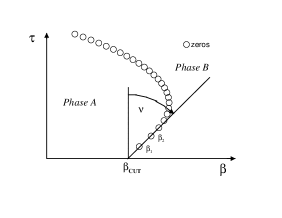
Figure 1: Schematic illustration of the zeros in the complex temperature plane.

The distribution of zeros close to the real axis can approximately be described by three parameters, where two of them reflect the order of the phase transition and the third merely the size of the system. We assume that the zeros lie on straight lines with a discrete density of zeros given by

$$\phi(\tau_{k})=\frac{1}{2}\left(\frac{1}{|{\cal B}_{k}-{\cal B}_{k-1}|}+\frac{1}{|{\cal B}_{k+1}-{\cal B}_{k}|}\right),$$ (2)

with $k=2,3,4,\cdots$, and approximate for small $\tau$ the density of zeros by a simple power law $\phi(\tau)\sim\tau^{\alpha}$. Considering only the first three zeros the exponent $\alpha$ can be estimated as

$$\alpha=\frac{\ln\phi(\tau_{3})-\ln\phi(\tau_{2})}{\ln\tau_{3}-\ln\tau_{2}}.$$ (3)

The second parameter describing the distribution of zeros is given by $\gamma=\tan\nu\sim(\beta_{2}-\beta_{1})/(\tau_{2}-\tau_{1})$ where $\nu$ is the crossing angle of the line of zeros with the real axis (see Fig. 1). The discreteness of the system is reflected in the imaginary part $\tau_{1}$ of the zero closest to the real axis. For macroscopic systems we always have $\tau_{1}\to 0$. In this case the parameters $\alpha$ and $\gamma$ match those defined by Grossmann et al. Gross1967 , who showed the connection between certain values of $\alpha$ and $\gamma$ and different types of phase transitions. They claimed that a first order transition occurs for $\alpha=\gamma=0$, for $0<\alpha<1$ with $\gamma=0$ or $\gamma\neq 0$ a second order transition, and for $\alpha>1$ a higher order transition. In the thermodynamic limit $\alpha$ is restricted to values greater than or equal to zero because otherwise this would cause a diverging internal energy. For finite systems values of $\alpha$ less than zero are possible.

In our classification scheme phase transitions in finite systems are of first order if $\alpha\leq 0$, while the definitions for higher order transitions coincide with those given by Grossmann. Additionally we define $\tau_{1}$ as an unambiguous parameter for the discreteness of the system. Since in small systems no thermodynamic properties diverge, the specification of the critical temperature is difficult and several definitions are possible which coincide only in the thermodynamic limit. We define the real part of the first zero $\beta_{1}$ as the critical temperature. Another possible definition would be the crossing point of the line of zeros with the real temperature axis.

III statistical multifragmentation model

In the statistical models for NMF Bondorf:1995 ; Chase:1994 ; Chase:1995 ; Mekjian:1991a it is assumed that the fragmentation process can be described in the following manner. After initial excitation the system expands and fragments into a number of clusters. During the expansion a thermalization of all clusters is assumed. The thermalization abruptly stops when the mean separation between the clusters exceeds the range of the nuclear force. The properties of the systems at this so-called freeze-out density, which is assumed to be 0.1-0.3 of the normal nuclear density $\rho_{0}=0.15$ fm^-3, are than carried by all fragments until experimental detection.

The probability for a fragmentation with fragmentation vector $\vec{n}=(n_{1},n_{2},\dots)$ ($n_{k}$ is the number of clusters of size $k$ and $\sum kn_{k}=A$), reads

$$W(\vec{n})=\prod_{k\geq 1}\frac{1}{n_{k}!}\left(\frac{xy^{k-1}}{\alpha_{k}}\right)^{n_{k}},$$ (4)

where $x=V_{\rm ac}\left(\frac{M}{2\pi\hbar^{2}{\cal B}}\right)^{3/2}$ is the partition function for the ideal monoatomic gas of mass $M$ in the accessible volume $V_{\rm ac}$. $y=\exp\big{(}a_{v}({\cal B}){\cal B}+\frac{T_{0}/\epsilon_{0}}{1+T_{0}{\cal B}}\big{)}$ is related to the cluster binding and internal excitations. The cluster size dependence of the probability is given by $\alpha_{k}=k^{5/2}$. We assume an accessible volume three times larger than the normal nucleus volume $V_{0}$. The canonical partition function is then given as

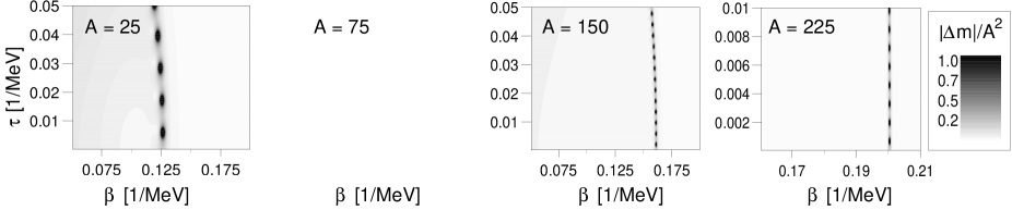
Figure 2: Contour plots of the variance of the multiplicity in the complex temperature plane for (a) A=25, (b) A=75, (c) A=150, and (d) A=225 nucleons. The dark spots indicate the locations of the zeros of $Z({\cal B})$.

$$Z_{A}=\sum_{m=0}^{A}Z_{A}^{(m)}x^{m}y^{A-m},$$ (5)

where $m=\sum_{k}n_{k}$ is the multiplicity, i.e. the total number of clusters, and $Z_{A}^{(m)}$ is independent of the thermodynamic variables and given by the simple recursion

$$Z_{A}^{(m)}=\frac{1}{m}\sum_{k=1}^{A}\frac{1}{\alpha_{k}}Z_{A-k}^{(m-1)},$$ (6)

with $Z_{A}^{(1)}=1/\alpha_{A}$.

Following Ref. Bondorf:1995 the binding energy for a composite of $k$ nucleons is given by

$$a_{v}({\cal B})=W_{0}k-\sigma({\cal B})k^{2/3},$$ (7)

with $\sigma({\cal B})=\sigma_{0}\left((T_{c}-1/{\cal B}^{2})/(T_{c}+1/{\cal B}^{2})\right)^{5/4}$ being the surface tension ($W_{0}=16$MeV, $\sigma_{0}=18$MeV, and $T_{c}=18$MeV).

Within this framework different moments of the multiplicity are calculated by

$$\left<m^{i}\right>=\frac{1}{Z_{A}}\sum_{m=0}^{A}m^{i}Z_{A}^{(m)}x^{m}y^{A-m}.$$ (8)

The variance of the multiplicity is given by $\Delta m=\langle m^{2}\rangle-\langle m\rangle^{2}$. It is straightforward to express thermodynamic quantities like the internal energy or the specific heat in terms of different moments of the multiplicity Chase:1995 .

IV results

Due to the unfavorable scaling behavior of the partition function it is very arduous to find its zeros directly with numerical methods. The zeros of $Z$ are the poles of almost all thermodynamic expectation values, e.g. the internal energy, the specific heat and so on. In this paper we utilize the absolute value of the variance of the multiplicity $|\langle\Delta m\rangle|$ to locate the zeros of $Z$ in the complex temperature plane. Fig. 2 shows a contour plot of $|\langle\Delta m\rangle|/A^{2}$ in the complex temperature plane for nucleon-numbers $A=25,75,150$, and $225$ (note the different scaling of the $\tau$-axis.). This figure directly shows that multifragmentation is a first order phase transition. The zeros lie on straight lines perpendicular to the real temperature axis with constant spacings between them. Even at particle numbers as small as 25 the nature of the phase transition can be clearly identified from the lines of zeros of the partition function.

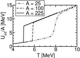
Figure 3: Canonical caloric curve for A=25, 100, and A=225.

In contrast, it is very difficult to extract the order of the phase transition from the canonical caloric curve (internal energy U_int per particle number A vs. temperature T) shown in Fig. 3.

The recursion formula (6) has a very similar structure to that for Bose-Einstein systems bf93 ; Borr99a ; Muelken:2000 . This is because both systems have an intimate relationship to the permutation group Mekjian:1991a . It is therefore remarkable, that the multifragmentation phase transition for nuclear matter is of first order while Bose-Einstein condensation is a second or third order phase transition depending on the single particle density of states.

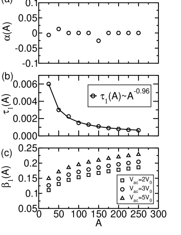
Figure 4: Nucleon number dependent value of the classification parameters (a) $\alpha$, (b) $\tau$ for an accessible volume $V_{\rm ac}=3V_{0}$ and (c) of the critical temperature $\beta_{1}$ for three different accessible volumes.

A detailed analysis of the distribution of zeros reveals that for all nucleon numbers ($A>25$) the most important classification parameter $\alpha$ is almost equal to zero (see Fig. 4(a)). The slight deviations for A=50 and A=150 are most likely due to uncertainties within our numerical zero detection method. The second parameter $\gamma$ can directly be extracted from Fig. 2. Even for small nucleon numbers the distribution of zeros is perpendicular to the real axis, corresponding to $\gamma=0$. The finite size of the system is connected to the third classification parameter $\tau_{1}$. Fig. 4(b) shows the $A$-dependence of $\tau_{1}$. With increasing nucleon number $\tau_{1}$ decreases. We approximated the scaling behavior as $\tau_{1}\sim A^{-0.96}$, i.e. $\tau_{1}$ is simply volume dependent and the phase transition would approach a true first order phase transition in the Ehrenfest sense with $1/A$. The critical temperature $T=1/\beta_{1}$ (Fig. 4(c)) decreases and adopts at $A\approx 200$ the experimentally found value of about $5$ MeV. Of course, for larger system sizes the simple equation (7) for the binding energy used in this study should be refined and augmented by additional terms. Additional calculations for different particle densities reveal that there are no qualitative changes to the first order nature of the phase transition. Fig. 4(c) also shows calculations for accessible volumes which are twice, three, and five times as large as the normal nucleus volume $V_{0}$. There are only quantitative changes in the critical temperature.

It should be noted that one can expect that refinements of the model, e.g. the introduction of an additional Coulomb term and other values of the particle density, may influence the details of the distribution of zeros. Especially tuning the particle density to the expected supercritical phase is an interesting challenge, worth to be pursued in the future.

V conclusion

In conclusion we have found that within the statistical model nuclear multifragmentation is undoubtedly a first order phase transition, which is in complete agreement with recent works based on micro-canonical and grand-canonical calculations Chomaz:2000 ; Bugaev:2000 . Of course, the first order type of the NMF phase transition is not yet sufficient to interprete NMF as the onset of the nuclear liquid-gas transition. However, this seems to be a necessary condition. The distribution of zeros of the partition function in the complex temperature plane proofs as a reliable tool for the classification of phase transitions, adding a clear, detailed, and unambiguous view on the thermodynamic properties of small systems.

- (1) R. Nenauer, A. J., and the INDRA collaboration, Nucl. Phys. A 658, 67 (1999), and references therein.
- (2) J. Pochodzalla, T. Möllenkamp, T. Rubehn, A. Schüttauf, W. A., E. Zude, M. Begemann-Blaich, T. Blaich, H. Emling, A. Ferrero, C. Gross, G. Imme, et al., Phys. Rev. Lett. 75, 1040 (1995).
- (3) Y.-G. Ma, A. Siwek, J. Peter, F. Gulminelli, R. Dayras, L. Nalpas, B. Tamain, E. Vient, G. Auger, C. Bacri, J. Benlliure, E. Bisquer, et al., Phys. Lett. B 390, 41 (1997).
- (4) X. Campi, Phys. Lett. B 208, 351 (1988).
- (5) W. Bauer and A. Botvina, Phys. Rev. C 52, 1750 (1995).
- (6) J. Aichelin and H. Stöcker, Phys. Lett. B 176, 14 (1986).
- (7) C. Hartnack, L. Zhuxia, L. Neise, G. Peilert, A. Rosenhauer, H. Sorge, J. Aichelin, H. Stöcker, and W. Greiner, Nucl. Phys. A 495, 303 (1989).
- (8) T. Maruyama, K. Niita, and A. Iwamoto, Phys. Rev. C 53, 297 (1996).
- (9) J. Bondorf, D. Idier, and I. Mishustin, Phys. Lett. B 359, 261 (1995).
- (10) G. Peilert, J. Konopka, M. Mustafa, H. Stöcker, and W. Greiner, Phys. Rev. C 46, 1457 (1992).
- (11) H. Feldmeier and J. Schnack, Rev. Mod. Phys. 72, 655 (2000).
- (12) J. Bondorf, B. A.S., A. Iljinov, I. Mishustin, and K. Sneppen, Phys. Rep. 257, 133 (1995).
- (13) D. Gross, Phys. Rep. 279, 119 (1995).
- (14) A. Parvan, V. Toneev, and M. Ploszajczak, Nucl. Phys. A 676, 409 (2000).
- (15) P. Bhattacharyya, S. Das Gupta, and A. Mekjian, Phys. Rev. C 60, 064625 (1999).
- (16) J. Elliott and A. Hirsch, Phys. Rev. C 61, 054605 (2000).
- (17) K. Chase and A. Mekjian, Phys. Rev. Lett. 75, 4732 (1995).
- (18) S. Lee and A. Mekjian, Phys. Rev. C 44, 1284 (1992).
- (19) A. DeAngelis and A. Mekjian, Phys. Rev. C 40, 105 (1989).
- (20) A. Mekjian, Phys. Rev. C 41, 2103 (1990).
- (21) S. Lee and A. Mekjian, Phys. Rev. C 47, 2266 (1993).
- (22) A. Mekjian and S. Lee, Phys. Rev. A 44, 6294 (1991).
- (23) K. Chase and A. Mekjian, Phys. Rev. C 49, 2164 (1994).
- (24) P. Borrmann, O. Mülken, and J. Harting, Phys. Rev. Lett. 84, 3511 (2000).
- (25) O. Mülken, P. Borrmann, J. Harting, and H. Stamerjohanns, arXiV:cond-mat/0006293 (2000).
- (26) S. Grossmann and W. Rosenhauer, Z. Phys. 207, 138 (1967); W. Bestgen, S. Grossmann, and W. Rosenhauer, J. Phys. Soc. Jap. 26, 115 (1969); S. Grossmann, Phys. Lett. 28A(2), 162 (1968); S. Grossmann and V. Lehmann, Z. Phys. 218, 449 (1969).
- (27) P. Borrmann and G. Franke, J. Chem. Phys 98, 2484 (1993).
- (28) P. Borrmann, J. Harting, O. Mülken, and E. Hilf, Phys. Rev. A 60, 1519 (1999).
- (29) Ph. Chomaz, V. Duflot, and F. Gulminelli, Phys. Rev. Lett. 85, 3587 (2000).
- (30) K. A. Bugaev, M. I. Gorenstein, I. N. Mishustin, and W. Greiner, arXiV:nucl-th/0007062 (2000).