Quantum Monte Carlo Methods for Nuclei at Finite Temperature

Abstract

We discuss finite temperature quantum Monte Carlo methods in the framework of the interacting nuclear shell model. The methods are based on a representation of the imaginary-time many-body propagator as a superposition of one-body propagators describing non-interacting fermions moving in fluctuating auxiliary fields. Fermionic Monte Carlo calculations have been limited by a “sign” problem. A practical solution in the nuclear case enables realistic calculations in much larger configuration spaces than can be solved by conventional methods. Good-sign interactions can be constructed for realistic estimates of certain nuclear properties. We present various applications of the methods for calculating collective properties and level densities.

1 Introduction

A variety of models have been developed over the years to explain the observed properties of nuclei in various mass regions. One of the more fundamental of these models is the interacting shell model, where valence nucleons (outside closed shells) move in a mean field potential and interact via a residual nuclear force. This effective interaction can be traced back to the bare nucleon-nucleon interaction via Brueckner’s $G$-matrix.

The nuclear shell model was applied successfully in the description of $p$[1], $sd$[2], and lower $pf$-shell nuclei[3, 4, 5]. However, the size of the model space increases combinatorially with the number of valence nucleons and/or orbitals, and conventional diagonalization of the nuclear Hamiltonian in a full shell is limited to nuclei up to $A\sim 50$.

At finite temperature many levels contribute, and diagonalization methods are even more limited. However, there are methods that do not require direct diagonalization of the Hamiltonian. At temperature $T$ the nucleus is described by its free energy $F(T)=-T\ln Z(T)$, where $Z(T)={\rm Tr}e^{-H/T}$ is the partition function expressed in terms of the nuclear Hamiltonian $H$. It is difficult to calculate the partition function because $H$ includes interactions that are strong, and non-perturbative methods are required. Thermal mean-field approximations, e.g., the Hartree-Fock approximation, are useful and tractable. Small amplitude fluctuations around the mean field can also be taken into account in the random phase approximation (RPA). However, in the finite nuclear system, large amplitude fluctuations are important. In fact, interaction effects can be taken into account exactly when all fluctuations of the mean field are properly included. This is formally expressed by the Hubbard-Stratonovich transformation.[6] In this transformation the nuclear propagator in imaginary time is represented as a superposition of one-body propagators that describe non-interacting fermions moving in fluctuating auxiliary fields. Quantum Monte Carlo methods were developed to carry out the integration over the large number of auxiliary fields.[7, 8] These calculations are computationally intensive and became feasible only with the introduction of parallel computers. Similar methods were developed for strongly correlated electron systems.[9, 10]

The initial applications of the Monte Carlo techniques were severely limited by the “sign” problem, which is generic to all fermionic Monte Carlo methods and occurs for all realistic nuclear interactions. We have developed a practical solution to this sign problem[8] that made possible realistic calculations in much larger configuration spaces than could be treated previously.

Other quantum Monte Carlo methods were developed for the many-nucleon system. Variational and Green function Monte Carlo methods were used successfully to derive properties of light nuclei from the bare nucleon-nucleon force.[11] Recently, a hybrid Monte Carlo method was suggested, in which the spin variables are decoupled using the Hubbard-Stratonovich transformation.[12]

The shell model Monte Carlo (SMMC) methods are reviewed in Section 2. Some of their applications are presented in Sections 3, 4 and 5.

2 Methods

2.1 The Hubbard-Stratonovich transformation

The shell model Hamiltonian contains a one-body part and a residual two-body interaction. A generic Hamiltonian with two-body interactions can be brought to the form

$$H=\sum_{a}\epsilon_{a}\hat{n}_{a}+\frac{1}{2}\sum_{\alpha}{v_{\alpha}}\hat{\rho}_{\alpha}^{2}\;,$$ (1)

where $\epsilon_{a}$ is the single-particle energy in orbital $a$, $\hat{\rho}_{\alpha}$ are linear combinations of one-body densities $\hat{\rho}_{ij}=a_{i}^{\dagger}a_{j}$, and $v_{\alpha}$ are interaction “eigenvalues.”

The canonical density operator $e^{-\beta H}$, where $\beta=1/kT$ is the inverse temperature, can also be viewed as the many-body evolution operator in imaginary time $\beta$. The Hubbard-Stratonovich (HS) transformation[6] is an exact representation of this propagator as a path integral over one-body propagators in fluctuating external fields $\sigma(\tau)$. It is derived by dividing the time interval $(0,\beta)$ into $N_{t}$ time slices of length $\Delta\beta$ each, and rewriting $e^{-\beta H}=\left(e^{-\Delta\beta H}\right)^{N_{t}}$. The propagator for each time slice can be written as $e^{-\Delta\beta H}\approx\prod_{a}e^{-\Delta\beta\epsilon_{a}\hat{n}_{a}}\prod_{\alpha}e^{-\frac{1}{2}{\Delta}\beta{v_{\alpha}}\hat{\rho}_{\alpha}^{2}}$ to order $({\Delta}\beta)^{2}$. Each factor with $\hat{\rho}_{\alpha}^{2}$ can be written as an integral over an auxiliary variable $\sigma_{\alpha}$

$$e^{-\frac{1}{2}{\Delta}\beta{v_{\alpha}}\hat{\rho}_{\alpha}^{2}}=\sqrt{{\beta|v_{\alpha}|}\over{2\pi}}\int d\sigma_{\alpha}e^{-\frac{1}{2}{\Delta}\beta|v_{\alpha}|{\sigma_{\alpha}^{2}}}e^{-{\Delta}\beta|v_{\alpha}|s_{\alpha}\sigma_{\alpha}\hat{\rho}_{\alpha}}\;,$$ (2)

where $s_{\alpha}=\pm 1$ for $v_{\alpha}<0$ and $s_{\alpha}=\pm i$ for $v_{\alpha}>0$. By introducing a different set of fields $\sigma_{\alpha}(\tau_{n})$ at each time slice $\tau_{n}=n\Delta\beta$, we obtain the HS representation of the propagator

$$e^{-\beta H}=\int{\cal D}[\sigma]G_{\sigma}U_{\sigma}\;,$$ (3)

where

$$G_{\sigma}=e^{-\frac{1}{2}{\Delta}\beta\sum_{\alpha,n}|v_{\alpha}|\sigma_{\alpha}^{2}(\tau_{n})}$$ (4)

is a Gaussian weight, and

$$U_{\sigma}=e^{-{\Delta}\beta h_{\sigma}(\tau_{n})}\ldots e^{-{\Delta}\beta h_{\sigma}(\tau_{1})}=T\exp{\left(-\int_{0}^{\beta}h_{\sigma}(\tau)d\tau\right)}$$ (5)

is the propagator of non-interacting nucleons moving in time-dependent external one-body auxiliary fields $\sigma_{\alpha}(\tau)$. The one-body Hamiltonian in (5) is given by

$$h_{\sigma}(\tau)=\sum_{a}\epsilon_{a}\hat{n}_{a}+\sum_{\alpha}s_{\alpha}|v_{\alpha}|\sigma_{\alpha}(\tau)\hat{\rho}_{\alpha}\;,$$ (6)

and the metric in the functional integral (3) is

$${\cal D}[\sigma]\equiv\Pi_{\alpha,n}\left[d\sigma_{\alpha}(\tau_{n})\sqrt{{{\Delta}\beta|v_{\alpha}|/{2\pi}}}\right]\;.$$ (7)

The thermal expectation of an observable $O$ can be represented from the HS transformation (3) as

$$\langle O\rangle={{\rm Tr}\,(Oe^{-\beta H})\over{\rm Tr}\,(e^{-\beta H})}={\int{\cal D}[\sigma]G_{\sigma}\langle O\rangle_{\sigma}{\rm Tr}\,U_{\sigma}\over\int{\cal D}[\sigma]G_{\sigma}{\rm Tr}\,U_{\sigma}}\;,$$ (8)

where $\langle O\rangle_{\sigma}\equiv{\rm Tr}\,(OU_{\sigma})/{\rm Tr}\,U_{\sigma}$ is the expectation value of $O$ for non-interacting particles moving in external fields $\sigma(\tau)$.

The calculation of the integrands in (8) can be reduced to matrix algebra in the single-particle space. To show that, we denote by $N_{s}$ the number of valence single-particle orbits, and represent the one-body propagator $U_{\sigma}$ in the single-particle space by an $N_{s}\times N_{s}$ matrix ${\bf U}_{\sigma}$. The grand-canonical trace of $U_{\sigma}$ in the many-particle fermionic space can be expressed directly in terms of ${\bf U}_{\sigma}$

$${\rm Tr}\;U_{\sigma}=\det({\bf 1}+{\bf U}_{\sigma})\;.$$ (9)

Eq. (9) is just the grand-canonical partition function of non-interacting fermions (moving in time-dependent external fields $\sigma$).

Similarly the grand-canonical expectation value of a one-body operator $O=\sum_{i,j}O_{ij}a^{\dagger}_{i}a_{j}$ can be calculated from

$$\langle a_{i}^{\dagger}a_{j}\rangle_{\sigma}=\left[{1\over{\bf 1}+{\bf U}^{-1}_{\sigma}}\right]_{ji}\;.$$ (10)

The grand-canonical expectation value of a two-body operator can be calculated using Wick’s theorem $\langle a^{\dagger}_{i}a^{\dagger}_{j}a_{l}a_{k}\rangle=\langle a^{\dagger}_{i}a_{l}\rangle\langle a^{\dagger}_{j}a_{k}\rangle-\langle a^{\dagger}_{i}a_{k}\rangle\langle a^{\dagger}_{j}a_{l}\rangle$ together with (10).

In practice, we are interested in canonical expectation values, for which the number of particles ${\cal A}$ is fixed. Canonical quantities can be calculated by an exact particle-number projection. The canonical (one-body) partition function is given as a Fourier transform[13]

$${\rm Tr}_{\cal A}U_{\sigma}=\frac{e^{-\beta\mu{\cal A}}}{N_{s}}\sum_{m=1}^{N_{s}}e^{-i\phi_{m}{\cal A}}\det\left[{\bf 1}+e^{i\phi_{m}}e^{\beta\mu}{\bf U}_{\sigma}\right]\;,$$ (11)

where $\phi_{m}=2\pi m/N_{s}\;\;(m=0,\ldots,N_{s})$ are quadrature points and $\mu$ is a chemical potential. Similarly for a one-body observable $O$

$${\rm Tr}_{\cal A}\left(OU_{\sigma}\right)=\frac{e^{-\beta\mu{\cal A}}}{N_{s}}\sum_{m=1}^{N_{s}}e^{-i\phi_{m}{\cal A}}\det\left[{\bf 1}+e^{i\phi_{m}+\beta\mu}{\bf U}_{\sigma}\right]{\rm tr}\;\left({1\over{\bf 1}+e^{-i\phi_{m}-\beta\mu}{\bf U}^{-1}_{\sigma}}{\bf O}\right)\;,$$ (12)

where ${\bf O}$ is the matrix with elements $O_{ij}$. In practical calculations it is necessary to project on both neutron number $N$ and proton number $Z$, and in the following ${\cal A}$ will denote $(N,Z)$.

2.2 Monte Carlo methods

The integrands in (8) are easily calculated by matrix algebra in the single-particle space (see, e.g., Eq. (9) and (10)). However, the number of integration variables $\sigma_{\alpha}(\tau)$ is very large. For small but finite $\Delta\beta$, this multi-dimensional integral can be evaluated exactly (up to a statistical error) by Monte Carlo methods.[7]

The first step is to define a positive-definite weight function

$$W_{\sigma}\equiv G_{\sigma}|{\rm Tr}\;U_{\sigma}|\;.$$ (13)

We can rewrite the expectation value (8) of an observable $O$ as

$$\langle O\rangle={\int D[\sigma]W_{\sigma}\Phi_{\sigma}\langle O\rangle_{\sigma}\over\int D[\sigma]W_{\sigma}\Phi_{\sigma}}\;,$$ (14)

where

$$\Phi_{\sigma}\equiv{\rm Tr}\;U_{\sigma}/|{\rm Tr}\;U_{\sigma}|$$ (15)

is the sign of the one-body partition function.

In the Monte Carlo approach, a random walk is performed in the space of auxiliary fields $\sigma\equiv\{\sigma_{\alpha}(\tau_{m})\}$ that samples the $\sigma$-fields according to the distribution $W_{\sigma}$. The $W$-weighted average of any $\sigma$-dependent quantity $X_{\sigma}$ can be estimated from

$$\langle X_{\sigma}\rangle_{W}\equiv{\int D[\sigma]W_{\sigma}X_{\sigma}\over\int D[\sigma]W_{\sigma}}\approx{1\over M}\sum_{k}X_{\sigma^{(k)}}\;,$$ (16)

where $\sigma^{(k)}$ are $M$ uncorrelated samples. The statistical error of $\langle X_{\sigma}\rangle_{W}$ can be estimated from the variance of the “measurements” $X_{\sigma^{(k)}}$. Though a standard random walk can be constructed by the Metropolis algorithm, a modification based on Gaussian quadratures improves the efficiency in the nuclear case.[14]

Using (14) and (16), thermal expectation values are calculated from

$$\langle O\rangle={\left\langle\langle O\rangle_{\sigma}\Phi_{\sigma}\right\rangle_{W}\over\langle\Phi_{\sigma}\rangle_{W}}\approx{\sum_{k}\langle O\rangle_{\sigma}\Phi_{\sigma}\over\sum_{k}\Phi_{\sigma}}\;.$$ (17)

Often the sign $\Phi_{\sigma}$ in (15) is not positive for some samples $\sigma$, and we must “measure” it together with the observable $\langle O\rangle_{\sigma}$.

2.3 The Monte Carlo sign problem

When the average sign $\langle\Phi_{\sigma}\rangle_{W}$ is smaller than its uncertainty, the Monte Carlo method fails. This leads to the so-called Monte Carlo “sign” problem: the sign of the integrand fluctuates among samples, and the integral is the result of a delicate cancellation that cannot be reproduced with a finite number of samples. Often the average sign decreases exponentially with $\beta$, and the problem becomes more severe at low temperatures. The sign problem is generic to all fermionic Monte Carlo methods[9] and has severely limited their applications. In particular, the problem occurs for all realistic effective interactions in the nuclear shell model. We have developed a practical solution to the sign problem in the nuclear case that allows realistic calculations in very large model spaces.[8]

Certain interactions can be shown to have a “good” sign. A time-reversal invariant Hamiltonian with two-body interactions can be written as

$$H=\sum_{a}\epsilon_{a}\hat{n}_{a}+{1\over 2}\sum_{\alpha}v_{\alpha}\left({\rho}_{\alpha}\bar{\rho}_{\alpha}+\bar{\rho}_{\alpha}{\rho}_{\alpha}\right)\;,$$ (18)

where $\bar{\rho}_{\alpha}$ is the time-reverse of ${\rho}_{\alpha}$ and $v_{\alpha}$ are real. When all $v_{\alpha}$ are negative in the representation (18), the grand-canonical partition function is positive-definite for any sample $\sigma$ and the interaction has a good sign. The proof is based on a generalization of Kramer’s degeneracy to the complex plane. The one-body Hamiltonian that appears in the HS decomposition for (18) has the form

$$h_{\sigma}=\sum_{a}\epsilon_{a}\hat{n}_{a}+\sum_{\alpha}\left(v_{\alpha}s_{\alpha}{\rho}_{\alpha}+v_{\alpha}s_{\alpha}\bar{\rho}_{\alpha}\right)\;.$$ (19)

When all $v_{\alpha}<0$, $s_{\alpha}=1$, and the Hamiltonian (19) is time-reversal invariant $\bar{h}_{\sigma}=h_{\sigma}$. The eigenstates of $\bf{U}_{\sigma}$ appear then in time-reversed pairs with complex conjugate eigenvalues $\{\lambda_{i},\lambda^{\ast}_{i}\}$, and the grand-canonical partition function ${\rm Tr}\;U_{\sigma}=\det(1+{\bf U}_{\sigma})=\Pi_{i}|1+\lambda_{i}|^{2}$ is positive-definite. The canonical partition function for even-even nuclei is also positive-definite.

Realistic effective nuclear interactions have both positive and negative “eigenvalues” $v_{\alpha}$, leading to a severe sign problem at low $T$. However, the eigenvalues that are large in magnitude are all negative and therefore have a good sign. This property of realistic nuclear forces can be used in several ways to overcome the sign problem.

In general, the Hamiltonian is decomposed into “good” and “bad” parts: $H=H_{G}+H_{B}$. The good Hamiltonian contains the one-body part plus the two-body terms with $v_{\alpha}<0$, while the bad Hamiltonian contains the two-body terms with $v_{\alpha}>0$. We construct a family of Hamiltonians

$$H_{g}=H_{G}+gH_{B}$$ (20)

that depends on a continuous coupling parameter $g$. For any $g<0$, the Hamiltonian (20) is good-sign and accurate Monte Carlo calculations can be performed for $\langle O\rangle_{g}\equiv{\rm Tr}\,(Oe^{-\beta H_{g}})/{\rm Tr}\,(e^{-\beta H_{g}})$. The dependence of $\langle O\rangle_{g}$ on $g$ is expected to be “smooth” and can therefore be extrapolated to $g=1$. We found, through tests in the $sd$- and lower $pf$-shell, that low-degree polynomial extrapolations (usually first or second order) are sufficient. The extrapolation technique is used in Section 3.

Certain nuclear properties such as collectivity and level densities can be reliably calculated by constructing nuclear Hamiltonians that are completely free of the sign problem.[15, 16] These Hamiltonians include correctly the dominating collective components of realistic effective interactions.[17] An example of a good-sign Hamiltonian, used in the applications discussed in Sections 4 and 5, is

$$H=\sum_{a}\epsilon_{a}\hat{n}_{a}-g_{0}P^{(0,1)\dagger}\cdot\tilde{P}^{(0,1)}-\chi\sum_{\lambda}k_{\lambda}O^{(\lambda,0)}\cdot O^{(\lambda,0)}\;,$$ (21)

where

$$P^{(\lambda,T)\dagger} = {\sqrt{4\pi}\over{2(2\lambda+1)}}\sum_{ab}\langle j_{a}\|Y_{\lambda}\|j_{b}\rangle[a_{j_{a}}^{\dagger}\times a_{j_{b}}^{\dagger}]^{(\lambda,T)}\;,$$

$$O^{(\lambda,T)} = {1\over\sqrt{2\lambda+1}}\sum_{ab}\langle j_{a}\|{{dV}\over{dr}}Y_{\lambda}\|j_{b}\rangle[a_{j_{a}}^{\dagger}\times\tilde{a}_{j_{b}}]^{(\lambda,T)}\;.$$ (22)

The modified annihilation operator is defined by $\tilde{a}_{j,m,m_{t}}=(-)^{j-m+{1\over 2}-m_{t}}a_{j,-m,-m_{t}}$, and a similar definition is used for $\tilde{P}^{(\lambda,T)}$. The single-particle energies $\epsilon_{a}$ are calculated from a Woods-Saxon potential plus spin-orbit interaction.[18] $V$ in (21) is the central part of this potential, and the multipole interaction is obtained by expanding the surface-peaked interaction $v({\bf r},{\bf r}^{\prime})=-\chi(dV/dr)(dV/dr^{\prime})\delta(\hat{\bf r}-\hat{\bf r}^{\prime})$. Since the monopole pairing and isoscalar multipole-multipole interactions are all attractive, they lead to a good-sign Hamiltonian (21).

Experimental gap parameters (found from odd-even mass differences) are used to determine the pairing strength $g_{0}$ through a particle-projected BCS calculation. The parameter $\chi$ of the surface-peak interaction is determined self-consistently: $\chi^{-1}=\int_{0}^{\infty}dr\;r^{2}\left(dV/dr\right)\left(d\rho/dr\right)$, where $\rho$ is the nuclear density. The renormalization factors $k_{\lambda}$ account for core polarization.

2.4 Particle-number reprojection

The SMMC methods are computationally intensive. Calculations can be done more efficiently in the particle-reprojection technique.[19] Suppose we use Monte Carlo methods to sample a nucleus with ${\cal A}$ particles. The ratio $Z_{{\cal A}^{\prime}}/Z_{\cal A}$ between the partition function of a nucleus with ${\cal A}^{\prime}$ particles and the partition function of the original nucleus can be calculated from

$${Z_{{\cal A}^{\prime}}(\beta)\over Z_{\cal A}(\beta)}\equiv{{\rm Tr}_{{\cal A}^{\prime}}e^{-\beta H}\over{\rm Tr}_{\cal A}e^{-\beta H}}=\left\langle{{\rm Tr}_{{\cal A}^{\prime}}U_{\sigma}\over{\rm Tr}_{\cal A}U_{\sigma}}\right\rangle_{W}\;,$$ (23)

where $\langle\ldots\rangle_{W}$ is defined in (16). Each of the partition functions within the brackets in (23) is calculated from (9). The expectation value of an observable $O$ for the nucleus with ${\cal A}^{\prime}$ particles is calculated using

$$\langle O\rangle_{{\cal A}^{\prime}}={\left\langle\left({{\rm Tr}_{{\cal A}^{\prime}}OU_{\sigma}\over{\rm Tr}_{{\cal A}^{\prime}}U_{\sigma}}\right)\left({{\rm Tr}_{{\cal A}^{\prime}}U_{\sigma}\over{\rm Tr}_{\cal A}U_{\sigma}}\right)\right\rangle_{W}\over\left\langle{{\rm Tr}_{{\cal A}^{\prime}}U_{\sigma}\over{\rm Tr}_{\cal A}U_{\sigma}}\right\rangle_{W}}\;.$$ (24)

In the particle-reprojection method, the Monte Carlo sampling is carried out by projecting on a nucleus with fixed ${\cal A}$, and the partition functions and observables are calculated for a family of nuclei with ${\cal A}^{\prime}\neq{\cal A}$ using Eqs. (23) and (24).

In the following Sections we present some of the applications of the shell model Monte Carlo approach.

3 Quenching of the Gamow-Teller strength

Gamow-Teller rates, especially in the iron region, are important inputs in models of stellar collapse and supernova formation.[20] They determine the electron-capture rates, which in turn affect the electron-to-baryon ratio.

The Gamow-Teller transition operator is given by

$$GT^{\pm}\propto\vec{\sigma}\tau_{\pm}\;,$$ (25)

where $\vec{\sigma}$ and $\vec{\tau}$ are the spin and isospin operators, respectively. The $GT^{+}$ transition operator changes a proton into a neutron, and its strength function can be measured in $(n,p)$ reactions.[21] The total strength $B(GT^{+})$ is found experimentally to be strongly quenched relative to estimates based on the independent-particle model.

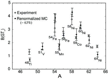
Figure 1: Total Gamow-Teller strength $B(GT^{+})$ in $pf$-shell nuclei. The solid symbols are the renormalized SMMC strengths and the open symbols are the experimental results. [21] After Ref. 23.

Calculations that include up to $2p-2h$ correlations account for some of the observed quenching.[22] To estimate how much of the quenching can be attributed to proton-neutron correlations in the ground state, we performed SMMC calculations in the complete $pf$-shell for nuclei in the iron region.[23] The total strength is renormalized by $(1/1.26)^{2}\sim 63\%$ to account for the normalization of the axial coupling constant from its free value of $g_{A}=1.26$ to $g_{A}=1$ in the nuclear medium. The renormalized strengths are shown in Fig. 1 in comparison with the experimental values. We see good agreement across the shell. We remark that a similar renormalization of the Gamow-Teller operator in complete $sd$-shell calculations also leads to an agreement with the data.[2]

We conclude that any observed quenching beyond an overall renormalization of $\sim 63\%$ is due to proton-neutron correlations. This has been confirmed in conventional shell model calculations in the $pf$-shell, where the Gamow-Teller strength is found to decrease as a function of the number of particle-hole excitations that are included in the model space.[24]

In SMMC it is also possible to calculate imaginary-time response functions and invert them by the maxent method to obtain strength functions.[7] Such methods were used to calculate Gamow-Teller strength distributions for $pf$-shell nuclei.[25]

4 $\gamma$-soft nuclei

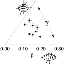
Figure 2: Free energy surfaces of ¹²⁴Xe and ¹²⁸Te at several temperatures. The surfaces are inferred from shape distributions calculated in SMMC. The inset on the right shows typical intrinsic shapes sampled in the Monte Carlo together with their standard deviation. After Ref. 15.

One of the outstanding problems in nuclear structure is to demonstrate that various types of collectivity (known from phenomenological models of nuclear structure) emerge in microscopic calculations. In particular, nuclei in the 100 – 140 mass region are known to be $\gamma$-soft, i.e., their potential energy is insensitive with respect to non-axial deformations. This region corresponds to the 50 – 82 shell (for both protons and neutrons), and could not be solved previously in fully microscopic calculations because of the prohibitively large size of the model space. Using SMMC we have provided the first microscopic evidence of softness in this mass region[15]. We have used the good-sign Hamiltonian (21) and, among the various multipole interactions, kept only an attractive quadrupole interaction renormalized to account for core polarization. A quadrupole pairing interaction (in addition to monopole pairing) was necessary to obtain correctly the excitation energy of the first $2^{+}$ state in tin isotopes.

To determine the quadrupole shape distribution $P(q_{\mu})$, we calculated for each sample $\sigma$ the average $\langle Q_{\mu}\rangle_{\sigma}$ and variance $\Delta_{\sigma}^{2}=\langle Q^{2}\rangle_{\sigma}-\langle Q\rangle_{\sigma}^{2}$ of the quadrupole mass operator $Q_{\mu}\equiv\sum r^{2}{\cal Y}_{2\mu}$. It is convenient to convert the shape distribution in the intrinsic frame $P(q^{\prime}_{0},q^{\prime}_{2})$ to an effective free energy surface at finite temperature using the relation[26] $P(q^{\prime}_{0},q^{\prime}_{2})dq^{\prime}_{0}dq^{\prime}_{2}\propto\exp\left[-F(\beta,\gamma;T)/T\right]\beta^{4}|\sin(3\gamma)|d\beta d\gamma$, where $\beta$ and $\gamma$ are the intrinsic quadrupole shape parameters. Such free energy surfaces are shown in Fig. 2 for ¹²⁸Te and ¹²⁴Xe at several temperatures. The inset shows typical intrinsic shapes, demonstrating the weak dependence of the free energy on $\gamma$.

5 Level densities

Level densities are important for theoretical estimates of nuclear reaction rates. In particular, level densities are necessary input for nucleosynthesis calculations. The $s$ and $r$ processes are determined by the competition between neutron capture and beta decay,[27] and the neutron-capture rates are proportional to the level density of the corresponding compound nucleus.[28]

Experimental data on level densities are available from different methods:[29] direct counting of levels at low energies, neutron and proton resonance data and charged particle spectra at intermediate energies, and Ericson’s fluctuations at higher energies.

Most conventional calculations of level densities are based on Fermi gas models in which important correlations are neglected. It is often found however, that empirical modifications of the Fermi gas formula (also known as Bethe’s formula[30]) can describe well experimental data. Particularly useful is the backshifted Bethe formula (BBF) where the ground state energy is backshifted by an amount $\Delta$. The backshift parameter originates in pairing correlations and shell effects. A modified version of the BBF is due to Lang and Le Couteur[31]

$$\rho(E_{x})\approx g{{\sqrt{\pi}}\over{24}}a^{-\frac{1}{4}}(E_{x}-\Delta+t)^{-\frac{5}{4}}e^{2\sqrt{a(E_{x}-\Delta)}}\;,$$ (26)

where $t$ is a thermodynamic temperature defined by $E_{x}-\Delta=at^{2}-t$ and $g=2$. The experimental level densities for many nuclei are well described by (26) when both $a$ and $\Delta$ are adjusted for each nucleus. It is therefore difficult to predict the level density to an accuracy better than an order of magnitude.

The nuclear shell model provides a suitable framework for the microscopic calculation of level densities. The dimensionality of the model space is often too large to allow for exact diagonalization, and truncations that might be appropriate for low-lying states are not suitable at finite excitation energies. Instead we use the Monte Carlo methods described in Section 2.

The calculations of level densities in SMMC[16] are based on a thermodynamic approach. The level density is obtained from the canonical partition function by an inverse Laplace transform

$$\rho(E)=\int_{-i\infty}^{i\infty}\frac{d\beta}{2\pi i}e^{\beta E}Z(\beta)\;.$$ (27)

In practice we are interested in the average level density. It can be obtained from (27) in the saddle point approximation

$$\rho(E)\approx(2\pi\beta^{-2}C)^{-1/2}e^{S}\;,$$ (28)

where the canonical entropy $S$ and heat capacity $C$ are given by

$$S=\ln Z+\beta E\;;\;\;\;C=\beta^{2}(\langle H^{2}\rangle-\langle H\rangle^{2})=-\beta^{2}\partial E/\partial\beta\;.$$ (29)

In SMMC we calculate the thermal energy $E(\beta)$ as an observable ($E(\beta)\equiv\langle H\rangle_{\beta}$), and then find the partition function by integrating the exact thermodynamic relation $E=-\partial\ln Z/\partial\beta$:

$$\ln\left[Z(\beta)/Z(0)\right]=-\int_{0}^{\beta}d\beta^{\prime}E(\beta^{\prime})\;.$$ (30)

$Z(0)={\rm Tr}~{}{\bf 1}$ is the total number of states in the model space. The entropy and heat capacity are then calculated from Eqs. (29) to give the level density (28).

5.1 Level densities in the iron region

We have used the methods of Section 5 to calculate level densities for nuclei in the iron region. The model space includes the $pf+g_{9/2}$-shell, and is good for excitation energies up to $E_{x}\sim 20$ MeV. With the inclusion of the $g_{9/2}$ orbit we can calculate both even and odd parity states.

We used the good-sign Hamiltonian (21) and kept only the quadrupole, octupole and hexadecupole terms with renormalization factors of $k_{2}=2$, $k_{3}=1.5$ and $k_{4}=1$. Using experimental odd-even mass differences we determined $g_{0}\approx 0.2$ MeV.

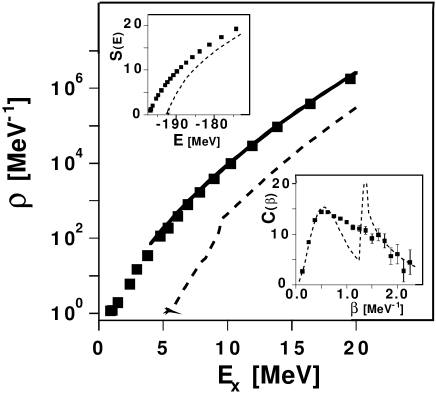
Figure 3: Total level density of ⁵⁶Fe versus excitation energy $E_{x}$: SMMC (solid squares), experiment (solid line) and HF (dashed line). The top inset shows the entropy $S(E)$, and the bottom inset is the heat capacity $C(\beta)$. The solid squares are the SMMC results while the dashed lines are obtained in the HF approximation. After Ref. 16.

Fig. 3 demonstrates the calculation of the level density of ⁵⁶Fe. The top and bottom insets show the entropy versus energy and the heat capacity versus $\beta$, respectively. For comparison we show the Hartree-Fock (HF) results by dashed lines. In the HF we observe a discontinuity in the heat capacity around $\beta\sim 1.3$ MeV^-1 due to a shape transition from a deformed to spherical nucleus. This discontinuity is washed out by the fluctuations in the SMMC calculations. The total SMMC level density for ⁵⁶Fe is shown in Fig. 3 versus excitation energy $E_{x}$ (solid squares). The solid line is inferred from the experiment.[32] We see good agreement between the microscopic calculations and the data, without any adjustable parameters.

The SMMC level density can be well-fitted to the BBF. We can therefore extract $a$ and $\Delta$ from the microscopic calculations. Fig. 4 shows the parameters $a$ (left) and $\Delta$ (right) as a function of mass number for even-even nuclei in the mass range $A\sim 50-70$.[33] The SMMC results (solid squares) are compared with the empirical values of Ref. 34 (solid lines). We observe that $a$ varies smoothly with mass, but that $\Delta$ shows shell effects and is enhanced at $N=28$ or $Z=28$.

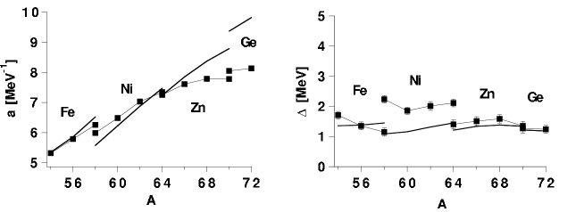
Figure 4: Single-particle level density parameter $a$ (left) and backshift parameter $\Delta$ (right) as a function of mass number $A$, obtained by fitting the SMMC level densities to the BBF. The solid lines are the empirical values of Ref. 34. Shown are results for even-even nuclei from Fe to Ge. After Ref. 33.

5.2 Level densities by particle-number reprojection

The projection on an odd number of particles introduces a new sign problem, even for good-sign Hamiltonians. Moreover, the calculations of level densities are time-consuming since each nucleus requires new Monte Carlo calculations for all temperatures.

The particle-number reprojection method of Section 2.4 can be used to carry out the Monte Carlo sampling for an even-even (or $N=Z$) nucleus ${\cal A}$ followed by a reprojection to find the thermal energies for a series of nuclei ${\cal A^{\prime}}$. We have applied this method to calculate the level densities of manganese, iron and cobalt isotopes by reprojecting from ⁵⁶Fe and ⁵⁴Co.[19] Since the Hamiltonian (21) depends on ${\cal A}$ (mostly through its single-particle spectrum), suitable corrections should be made to the thermal energy.

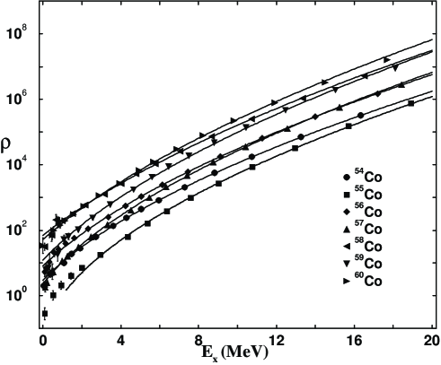
Figure 5: Level densities of cobalt isotopes versus excitation energies obtained in the particle-number reprojection method. The solid lines are fits to the BBF formula (26). After Ref. 19.

Results for the level densities of cobalt isotopes, reprojected from ⁵⁶Fe, are shown in Fig. 5. We observe that the level density of an odd-odd cobalt (e.g., ⁵⁴Co) is higher than the level density of the subsequent even-odd cobalt (⁵⁵Co) although the latter has a larger mass. The systematics of $a$ and $\Delta$ is shown in Fig. 6 for manganese, iron and cobalt isotopes, including odd-$A$ and odd-odd nuclei. The SMMC results (solid squares) are compared with the experimental values (x’s) and the empirical formulas of Ref. 34 (solid lines). The staggering effect in $\Delta$ originates in pairing correlations. The microscopic calculations are often in better agreement with the data than are the empirical values.

Figure 6: The single-particle level density parameter $a$ (left) and backshift parameter $\Delta$ (right) in manganese, iron and cobalt isotopes. The values determined by particle-number reprojection SMMC (solid squares) are compared with the experimental values (x’s) [29] and the empirical values of Ref. 34 (solid lines). After Ref. 19.

5.3 Parity-projected level densities

We have calculated the parity dependence of level densities by introducing parity projection in the HS representation. The projection operators on even- and odd-parity states are given by $P_{\pm}=(1\pm P)/2$, where $P$ is the parity operator. The parity-projected thermal energies $E_{\pm}(\beta)\equiv{{\rm Tr}(HP_{\pm}e^{-\beta H})/{\rm Tr}(P_{\pm}e^{-\beta H})}$ can be written as

$$E_{\pm}(\beta)={\int D[\sigma]W_{\sigma}\Phi_{\sigma}\left[\langle H\rangle_{\sigma}\pm\langle H\rangle_{P\sigma}\zeta_{P}(\sigma)/\zeta(\sigma)\right]\over\int D[\sigma]W_{\sigma}\Phi_{\sigma}\left[1\pm{\zeta_{P}(\sigma)/\zeta(\sigma)}\right]}\;,$$ (31)

where $\zeta(\sigma)\equiv{\rm Tr}\;U_{\sigma}$, $\zeta_{P}(\sigma)\equiv{\rm Tr}\;(PU_{\sigma})$ and $\langle H\rangle_{P\sigma}\equiv{\rm Tr}\;(HPU_{\sigma})/{\rm Tr}\;(PU_{\sigma})$. $PU_{\sigma}$ can be represented in the single-particle space by the matrix ${\bf P}{\bf U}_{\sigma}$, where ${\bf P}$ is a diagonal matrix with elements $(-)^{\ell_{a}}$ ($\ell_{a}$ is the orbital angular momentum of the single-particle orbit $a$). Consequently, the integrand in (31) can be calculated by matrix algebra in the single-particle space. From $E_{\pm}(\beta)$ we calculate the positive- and negative-parity level densities using the method discussed in Section 5.

The left panel of Fig. 7 shows the parity-projected level densities for ⁵⁶Fe. We see that $\rho_{+}\neq\rho_{-}$ even at the neutron resonance energies. This is contrary to the common assumption of equal even and odd parity densities, often used in nucleosynthesis calculations.

It is difficult to calculate the odd-parity level density for the even-even nuclei at low excitation energies because of a new sign problem introduced by the projection $P_{-}$. The sign problem affects less the odd-to-even partition function ratio. This ratio is calculated from

$${Z_{-}\over Z_{+}}=\left.\left[1-\left\langle{\zeta_{P}(\sigma)\over\zeta(\sigma)}\right\rangle_{W}\right]\right/\left[1+\left\langle{\zeta_{P}(\sigma)\over\zeta(\sigma)}\right\rangle_{W}\right]\;,$$ (32)

and shown in the right panel of Fig. 7 for several nuclei in the iron region.

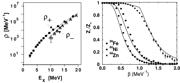
Figure 7: Left: parity projected level densities $\rho_{\pm}$ in ⁵⁶Fe. Right: odd-to-even partition function ratio versus $\beta$ for ⁵⁶Fe, ⁶⁰Ni and ⁶⁸Zn. The symbols are the SMMC calculations and the solid lines are obtained from Eq. (33) of the statistical quasi-particle model (see text). After Refs. 16 and 35.

The parity distribution as a function of temperature (or excitation energy) can be understood in terms of a simple statistical model.[35] The single-particle states are divided into two groups of odd- and even-parity states. Assuming that the particles occupy the single-particle states randomly and independently, the probability to find $n$ nucleons in states with parity $\pi$ ($\pi$ is the parity of the group with the smaller occupation) is a Poisson distribution, $P(n)=f^{n}e^{-f}/n!$, where $f=\langle n\rangle$. For an even-$A$ nucleus, an even (odd) parity many-particle state is obtained when $n$ is even (odd). We find a simple formula for the odd-to-even parity ratio

$${Z_{-}(\beta)\over Z_{+}(\beta)}={\sum_{n\;\rm odd}P(n)\over\sum_{n\;\rm even}P(n)}=\tanh f\;.$$ (33)

$f$ is estimated from the Fermi-Dirac occupations of deformed single-particle states with parity $\pi$. The distribution $P(n)$ can be calculated in SMMC by projection on states with parity $\pi$[35]. In the iron region we find good agreement with the Poisson distribution above the pairing transition temperature of $\sim 1$ MeV. Below this temperature, our model is still valid but for the quasi-particles. $f$ is now given by[36] $f=\sum_{a\in\pi}f_{a}=\sum_{a\in\pi}[1+e^{\beta E_{a}}]^{-1}$ where $E_{a}=\sqrt{(\epsilon_{a}-\lambda)^{2}+\Delta^{2}}$ are the quasi-particle energies (and $\lambda$ is the chemical potential). The solid lines in Fig. 7 are the result (33) of the quasi-particle model.

Conclusions

We have discussed a quantum Monte Carlo approach to the interacting shell model at finite and zero temperature. The initial applications of these techniques have been severely limited by the Monte Carlo sign problem. A practical solution to the sign problem in the nuclear case has allowed new realistic calculations that could not be carried out in conventional diagonalization methods. Alternatively, good-sign interactions can be constructed for realistic estimates of certain nuclear properties (e.g., collective properties and level densities). We have presented a variety of applications: the quenching of the Gamow-Teller strength, microscopic evidence of $\gamma$-softness, and accurate calculations of level densities and their parity distribution.

Finally, it is important to keep in mind that the Monte Carlo approach is complementary to the conventional shell model approach; it cannot be used to calculate detailed spectra but on the other hand it is very useful for finite and zero temperature calculations.

References

- [1] S. Cohen and D. Kurath, Nucl. Phys. 73, 1 (1965).
- [2] B. H. Wildenthal, Prog. Part. Nucl. Phys. 11, 5 (1984); B.A. Brown and B.H. Wildenthal, Ann. Rev. Nucl. Part. Sci. 38, 29 (1988).
- [3] W. A. Richter, M.G. Vandermerwe, R.E. Julies, and B.A. Brown, Nucl. Phys. A523, 325 (1991).
- [4] E. Caurier, A. P. Zuker, A. Poves and G. Martinez-Pinedo, Phys. Rev. C 50, 225 (1994); G. Martinez-Pinedo, A. P. Zuker, A. Poves and E. Caurier, Phys. Rev. C 55, 187 (1997).
- [5] A. Novoselsky, M. Vallières and O. La’adan, Phys. Rev. Lett. 79, 4341 (1997); A. Novoselsky and M. Vallières, Phys. Rev. C 57, R19 (1998).
- [6] J. Hubbard, Phys. Rev. Lett. 3, 77 (1959); R. L. Stratonovich, Dokl. Akad. Nauk. S.S.S.R. 115, 1097 (1957).
- [7] G. H. Lang, C. W. Johnson, S. E. Koonin, and W. E. Ormand, Phys. Rev. C 48, 1518 (1993).
- [8] Y. Alhassid, D. J. Dean, S. E. Koonin, G. Lang, and W. E. Ormand, Phys. Rev. Lett. 72, 613 (1994).
- [9] E. Y. Loh, Jr. and J. E. Gubernatis, in Electronic Phase Transitions, edited by W. Hanke and Y. V. Kopaev (North Holland, Amsterdam, 1992).
- [10] W. von der Linden, Phys. Reports 220, 53 (1992).
- [11] B.S. Pudliner, V.R. Pandharipande, J. Carlson, and R.B. Wiringa, Phys. Rev. Lett. 74, 4396 (1995); B.S. Pudliner, V.R. Pandharipande, J. Carlson, S.C. Pieper and R.B. Wiringa, Phys. Rev. C 56, 1720 (1997).
- [12] K.E. Schmidt and S. Fantoni, Phys. Lett. B 446, 99 (1999).
- [13] W. E. Ormand, D. J. Dean, C. W. Johnson, G. H. Lang and S. E. Koonin, Phys. Rev. C 49, 1422 (1994).
- [14] D. J. Dean, S.E. Koonin, G. H. Lang, P.B. Radha and W. E. Ormand, Phys. Lett. B 317, 275 (1993).
- [15] Y. Alhassid, G. F. Bertsch, D. J. Dean, and S. E. Koonin, Phys. Rev. Lett. 77, 1444 (1996).
- [16] H. Nakada and Y. Alhassid, Phys. Rev. Lett. 79, 2939 (1997).
- [17] M. Dufour and A.P. Zuker, Phys. Rev. C 54, 1641 (1996).
- [18] A. Bohr and B. R. Mottelson, Nuclear Structure vol. 1 (Benjamin, New York, 1969), p. 238.
- [19] Y. Alhassid, S. Liu and H. Nakada, Phys. Rev. Lett. 83, 4265 (1999).
- [20] H.A. Bethe, Rev. Mod. Phys. 62, 801 (1990).
- [21] M.C. Vetterli et al., Phys. Rev. C 40, 559 (1989); W.P. Alford et al., Nucl. Phys. A 514, 49 (1990); T. Rönnqvist et al., Nucl. Phys. A 563, 225 (1993); S. El-Kateb et al., Phys. Rev. C 49, 3129 (1994); A.L. Williams et al., Phys. Rev. C 51, 1144 (1995).
- [22] N. Auerbach, G. F. Bertsch, B. A. Brown, and L. Zhao, Nucl. Phys. A556, 190 (1993).
- [23] K. Langanke, D. J. Dean, P. B. Radha, Y. Alhassid, and S. E. Koonin, Phys. Rev. C52, 718 (1995).
- [24] E. Caurier, G. Martinez-Pinedo, A. Poves and A.P. Zuker, Phys. Rev. C 52, R 1746 (1996).
- [25] P.B. Radha, D.J. Dean, S.E. Koonin, K. Langanke and P. Vogel, Phys. Rev. C 56, 3079 (1997).
- [26] Y. Alhassid, in New Trends in Nuclear Collective Dynamics, Y. Abe ed., Springer Verlag, NY (1992); Y. Alhassid, Nucl. Phys. A 553, 137c (1993), and references therein.
- [27] E.M. Burbidge, G.R. Burbidge, W.A. Fowler and F. Hoyle, Rev. Mod. Phys. 29, 547 (1957).
- [28] T. Rauscher, F.-K. Thielemann and K.-L. Kratz, Phys. Rev. C 56, 1613 (1997).
- [29] W. Dilg, W. Schantl, H. Vonach and M. Uhl, Nucl. Phys. A217, 269 (1973), and references therein.
- [30] H. A. Bethe, Phys. Rev. 50, 332 (1936).
- [31] J.M.B. Lang and K.J. LeCouteur, Proc. Phys. Soc. (London) A 67, 585 (1954).
- [32] C.C. Lu, L.C. Vaz and J.R. Huizenga, Nucl. Phys. A 190, 229 (1972).
- [33] H. Nakada and Y. Alhassid, Phys. Lett. B 436, 231 (1998).
- [34] J. A. Holmes, S. E. Woosley, W. A. Fowler and B. A. Zimmerman, Atom. Data and Nucl. Data Tables 18, 305 (1976); S. E. Woosley, W. A. Fowler, J. A. Holmes and B. A. Zimmerman, Atom. Data and Nucl. Data Tables 22, 371 (1978).
- [35] Y. Alhassid, G.F. Bertsch, S. Liu and H. Nakada, Phys. Rev. Lett. 84, 4313 (2000).
- [36] J. Bardeen, L.N. Cooper and J.R. Schrieffer, Phys. Rev. 108, 1175 (1957).