Coulomb exchange and pairing contributions in nuclear Hartree–Fock–Bogoliubov calculations with the Gogny force

Abstract

We present exact Hartree–Fock–Bogoliubov calculations with the finite range density dependent Gogny force using a triaxial basis. For the first time, all contributions to the Pairing and Fock Fields arising from the Gogny and Coulomb interactions as well as the two-body correction of the kinetic energy have been calculated in this basis. We analyze the relevance of these terms in different regions of the periodic table at zero and high angular momentum. The validity of commonly used approximations that neglect different terms in the variational equations is also checked. We find a decrease of the proton pairing energies mainly due to a Coulomb antipairing effect.

1 Introduction

The mean field approximation is the backbone of many-body calculations in Nuclear Physics, either as a zero order approach to the problem or as a basis for more elaborated theories like the Random-Phase approximation or the Generator Coordinate Method. The modern and fast computer facilities have made possible the use of effective density dependent interactions, as the Skyrme [1] or the Gogny force [2], in standard mean field calculations like the Hartree-Fock (HF) or the Hartree-Fock-Bogoliubov (HFB) approaches.

In spite of the relative simplicity of the mean field approach, some additional approximations have been commonly used when effective forces were used in the mean field calculations in order to make the problem more tractable. The complications in the calculations usually arise from the exchange terms, either from the Coulomb force or from some components of the nuclear force itself. Depending on the mean field approach (HF or HFB) and on the force (zero or finite range) different approximations have been used in the past. In the HF theory one has only one exchange term (the Fock term) which contributes to the HF field. Commonly, in this type of calculations, in order to retain the required simplicity of the model, the Fock term of the Coulomb force has been neglected, or treated in the Slater approximation. In ref. [3] the validity of different approaches for the Coulomb Fock contribution was tested in HF calculations finding the Slater approximation a good one. In the HFB approach, and for any two-body interaction, one has two exchange terms, the Fock term which contributes to the HF field and the particle-particle (pp) term which contributes to the pairing field. In the HFB approach one must distinguish between the Skyrme and the Gogny force. Since the Skyrme force is assumed to provide only the particle-hole (ph) part of the force, all terms of the pp type are neglected even those arising from the Coulomb force. With the Gogny force the situation is different because with its finite range it has been designed to provide both, the ph and the pp part of the nuclear force.

A test similar to the one performed for HF in ref. [3] has never been done for HFB calculations. Exact HFB calculations with the Gogny force have been performed for spherical nuclei [2], but the effects of the approximation of neglecting the exchange terms never have been analyzed. For the more complex triaxial HFB calculations it has been assumed that the findings of ref. [3] for the HF approach, concerning the exchange terms, will also apply to this case. This point, however, never has been checked.

HFB calculations with triaxial symmetry using density–dependent interactions like the Gogny force, used by different groups [4, 5, 6], are usually performed using the following approximations:

• First, the contributions to the pairing field stemming from the center of mass correction, Coulomb and spin–orbit terms are neglected. This is motivated by the fact that their contribution, in the limit of axial deformations, is assumed (but not proved) to be negligible small [4]. Thus, under these conditions the pairing field arises only from the Brink–Boeker term.

• Second, since the exchange (Fock) Coulomb term contribution to the HF field requires a large CPU time, its contribution to the energy is not taken into account or it is included in the Slater approximation.

On the other hand in the HFB theory, pairing is an important degree of freedom and it is important to analyze how the properties related to this part of the field change when some approximations are assumed. In this paper, for the first time, we calculate in the triaxial basis the contributions mentioned above . We shall investigate the effect of including all the terms in the fields as compared with the calculations which are normally done for deformed nuclei. Mainly the D1S parameterization of the Gogny force [8] is used in the calculations, though some calculations with the D1 [2, 9] parameterization will be done. We shall study nuclei which have been analyzed by the approximate triaxial HFB, like some nuclei in the rare earth region [5, 10], in the superdeformed A$\approx 190$ region [6] and in the actinide region [4]. In the same way, we shall also analyze these contributions in spherical nuclei in order to understand how the results obtained depend on the basis used. A brief review of the method is given in Sect. 2. The effect of the different contributions in spherical nuclei is studied in Sect. 3.1 for the N$=50$ region and in Sect. 3.2 for the N$=82$ y N$=126$ regions. The rare earth region will be analyzed in the Sect. 4.1. The effect of the new terms in the nucleus ²⁴⁰Pu (actinide region) will be treated in Sect. 4.2. The behavior of a nucleus in the superdeformed region $A\approx 190$ will be studied in Sect. 5. Finally an study of energy surfaces with considerations of the exchange terms will be done in Sec. 6. A discussion and the conclusions will be presented at the end of the paper.

2 Theory

The HFB theory [11] unifies the self–consistent description of nuclear orbitals, as given by the Hartree–Fock (HF) approach and the Bardeen–Cooper–Schrieffer (BCS) pairing theory into a single variational theory. As trial wave function an independent quasiparticle state $|\Phi\rangle$ is considered. This wave function is a linear combination of independent multi-particle states representing various possibilities of occupying single–particle states. The quasiparticle operators are defined by

$$\alpha_{\mu}=\sum_{i}U_{i\mu}^{*}c_{i}+V_{i\mu}^{*}c_{i}^{\dagger},$$ (1)

with ${c_{k}^{\dagger},c_{k}}$ the particle creation and annihilation operators in the harmonic oscillator basis and $U$ and $V$ the Bogoliubov wave functions to be determined by the Ritz variational principle. The corresponding equations have been solved by the Conjugate Gradient Method [12]. The Bogoliubov transformation (1) leads to wave functions $|\Phi\rangle$ that are not eigenstates of the particle number operator. Furthermore, to generate a wave function $|\Phi_{I}\rangle$ corresponding to a rotational state with angular momentum $I$ we shall use the cranking prescription. Therefore, in the minimization process one has to add Lagrange multipliers to satisfy the pertinent constraints. That means, the wave function $|\Phi_{I}\rangle$ is determined by the condition

$$\delta\langle\Phi_{I}|\hat{H}-\omega\hat{J}_{x}-\lambda_{N}\hat{N}-\lambda_{Z}\hat{Z}|\Phi_{I}\rangle=0$$ (2)

with the Lagrange multipliers $\omega,\lambda_{N}$ and $\lambda_{Z}$ determined by the usual constraints $\langle\hat{J}_{x}\rangle=\sqrt{I(I+1)}$, $\langle\hat{N}\rangle=N$ and $\langle\hat{Z}\rangle=Z$, in an obvious notation.

In the second quantization formalism, the nuclear Hamiltonian is given by

$$\hat{H}=\sum_{k_{1}k_{2}}t_{k_{1}k_{2}}c_{k_{1}}^{\dagger}c_{k_{2}}\,+\,\frac{1}{2}\sum_{k_{1}k_{2}k_{3}k_{4}}{v}_{k_{1}k_{2}k_{3}k_{4}}c_{k_{1}}^{\dagger}c_{k_{2}}^{\dagger}c_{k_{4}}c_{k_{3}}.$$ (3)

where $t$ is the kinetic energy and $v$ the two-body interaction, $\bar{v}$ if antisymmetrized. The Wick theorem allows the evaluation of the expectation value of a two-body operator in a simple way:

$$\langle c_{k_{1}}^{\dagger}c_{k_{2}}^{\dagger}c_{k_{4}}c_{k_{3}}\rangle=\langle c_{k_{1}}^{\dagger}c_{k_{3}}\rangle\langle c_{k_{2}}^{\dagger}c_{k_{4}}\rangle\,-\,\langle c_{k_{2}}^{\dagger}c_{k_{3}}\rangle\langle c_{k_{1}}^{\dagger}c_{k_{4}}\rangle\,+\,\langle c_{k_{1}}^{\dagger}c_{k_{2}}^{\dagger}\rangle\langle c_{k_{4}}c_{k_{3}}\rangle,$$ (4)

where we have introduced the shorthand notation $\langle\Phi|\hat{O}|\Phi\rangle\equiv\langle\hat{O}\rangle$ for the expectation value of any operator $\hat{O}$. The first term on the r.h.s. of eq. (4) is called the Hartree term, the second one the Fock term and the third one the pairing term. Using the expressions

$$\rho_{k_{1},k_{2}}=\langle c_{k_{2}}^{\dagger}c_{k_{1}}\rangle,\;\;\;\;\kappa_{k_{1},k_{2}}=\langle c_{k_{2}}c_{k_{1}}\rangle,$$ (5)

for the density matrix $\rho$ and the pairing tensor $\kappa$, and

$$\Gamma_{k_{1}k_{3}}=\sum_{k_{2}k_{4}}\bar{v}_{k_{1}k_{2}k_{3}k_{4}}\rho_{k_{4}k_{2}},\quad\Delta_{k_{1}k_{2}}=\frac{1}{2}\sum_{k_{3}k_{4}}\bar{v}_{k_{1}k_{2}k_{3}k_{4}}\kappa_{k_{3}k_{4}},$$ (6)

for the HF field $\Gamma$ and the pairing field $\Delta$, we can express the expectation value of the nuclear Hamiltonian by

$$E=\langle\hat{H}\rangle={\displaystyle Tr}(t\rho)+\frac{1}{2}{\displaystyle Tr}\left(\Gamma\rho\right)-\frac{1}{2}{\displaystyle Tr}\left(\Delta{\kappa}^{*}\right).$$ (7)

The second addend in this expression arises from the contributions of the Hartree and the Fock terms of eq. (4) while the third one stems from the pairing term of eq. (4). The two-body effective nuclear interaction $v$ used in our calculations, see Appendix A, is made up from the Gogny force, the Coulomb (C) interaction and the two–body correction of the kinetic energy (TK). The Gogny force itself has the following terms: Brink–Boeker (BB), spin–orbit (SO) and density–dependent (DD) contributions. Then, the total HFB energy can be written as

$$E={\displaystyle Tr}(t\rho)+V_{BB}+V_{SO}+V_{DD}+V_{TK}+V_{C}$$ (8)

where we have written separately the different energy contributions. Each contribution, $V_{L}$, is calculated from the corresponding Hartree–Fock, $\Gamma_{L}$, and pairing, $\Delta_{L}$, fields (L $\equiv$ BB, SO, DD, TK or C) and is given by

$$V_{L}=\frac{1}{2}{\displaystyle Tr}\,\left(\Gamma_{L}\rho-\Delta_{L}\kappa^{*}\right)=V_{L}^{H}+V_{L}^{F}+V_{L}^{P}$$ (9)

where $\Gamma_{L}$ and $\Delta_{L}$ are given by eq. (6) but considering, instead of the full interaction $v$, only the part $L$ of the force. On the r.h.s. of this expression we have further separated $V_{L}$ into the three contributions obtained from each of the terms of eq. (4), namely, the Hartree-, the Fock- and the pairing term.

As mentioned above, in HFB calculations with the Gogny force and a triaxial basis several approximations have been done. In particular the contributions to the pairing field from the spin–orbit, two–body correction of the kinetic energy and Coulomb terms have been usually neglected in the self–consistent procedure. Furthermore, the exchange contribution of the Coulomb potential (Fock term) to the Hartree–Fock field has not been taken into account in most of the cases or treated in the Slater approximation. Thus, in the simplest HFB approximation, which we shall denote HFB_s ($s$ for standard), the HFB energy used in the variational process is given by

$$E_{s}={\displaystyle Tr}(t\rho)+V_{BB}+V_{DD}+\frac{1}{2}{\displaystyle Tr}\left(\,(\Gamma_{SO}+\Gamma_{TK}+\Gamma^{H}_{C})\rho\,\right)$$ (10)

A first order perturbation theory correction to this approach, which we shall denote HFB_s+, is to calculate the neglected terms just at the end of the iterative procedure and to add them to the total energy. We shall test, in different mass regions, how good this approach is with respect to the exact calculation (7), denoted HFB_e ($e$ for exact), and with respect to other approaches that we shall introduce later on. Details on the calculation of the terms neglected in the HFB_s approximation but included in the exact one are given in Appendix B.

The triaxial basis used in the calculations is spanned by harmonic oscillator states with quantum numbers $\{n_{x},n_{y},n_{z}\}$ which fulfill the condition, $a_{x}n_{x}+a_{y}n_{y}+a_{z}n_{z}\leq N_{0}$. The coefficients $a_{i}$ are related to the axis of the nuclear matter distribution by $a_{x}={(qp)}^{1/3}$, $a_{y}=q^{1/3}p^{-2/3}$ and $a_{z}=p^{1/3}q^{-2/3}$ [4].

3 Spherical nuclei

In this section we concentrate mainly on the effect of the Coulomb contribution in HFB calculations for spherical nuclei. We are interested to know the behavior of the pairing and total energies when different approximations for the Coulomb terms are used. At the end of sect. 3.1, a short discussion is devoted to the contributions to the total energy of the pairing field of both, the spin–orbit term and the two–body correction of the kinetic energy term.

3.1 N$=50$ region

In this subsection we shall study the medium heavy nuclei from the region $N=50$. We shall use the basis determined by $q=1.0$, $p=1.0$ and $N_{0}=11.1$. In the calculations the D1S parameterization of the Gogny force has been used. First we analyze in detail the Coulomb terms and ignore for the moment the SO and TK pairing exchange terms.

The Coulomb interaction contributes to the energy with three terms : The Hartree (H / h) or direct term, the Fock (F / f) or exchange term and the pairing (P / p) or Bogoliubov term. Each term can be considered either selfconsistently, i.e., taken into account in the variational process, or non-selfconsistently (perturbationally), i.e., ignored during the variation but its value being added to the total energy at the end of the variational process. In the first case we shall use capital letters (H, F or P) and in the second one small letters (h, f or p) to label the approximation used for the respective terms. For example the approximation $Hfp$ means that the Hartree Coulomb term has been taken into account selfconsistently and the Fock and Pairing Coulomb terms only perturbationally. To understand which contributions are more important and the convenience of considering in the variational process the pertinent terms we shall investigate the following approximations:

In the simplest calculation the three Coulomb terms mentioned above, i.e., even the Coulomb Hartree term, are neglected. In this approximation the energy, which we shall call reference energy, $E_{ref}$, given by

$$E_{ref}={\displaystyle Tr}(t\rho)+V_{BB}+V_{DD}+\frac{1}{2}{\displaystyle Tr}\left(\,(\Gamma_{SO}+\Gamma_{TK})\rho\,\right)$$ (11)

is considered in the minimization process. The next approximations will be

$$E_{hfp} = E_{ref}+[V_{C}]$$ (12)

$$E_{Hfp} = E_{ref}+V_{C}^{H}+[V_{C}^{F}+V_{C}^{P}]$$ (13)

$$E_{HFp} = E_{ref}+V_{C}^{H}+V_{C}^{F}+[V_{C}^{P}]$$ (14)

$$E_{HFP} = E_{ref}+V_{C}$$ (15)

We use squared brackets to indicate the terms considered perturbationally, the others, are used in the variational equations. Notice, therefore, that only the latter ones determine the wave function. To remember the meaning of each approximation one just needs to look at the subindex of the energy and to keep in mind the convention introduced above about capital and small letters. We shall also investigate the Slater approximation used by several groups. In this case the energy looks like

$$E_{H\tilde{F}p}=E_{ref}+V_{C}^{H}+\tilde{V}_{C}^{F}+[V_{C}^{P}]$$ (16)

In $E_{H\tilde{F}p}$ the tilde on $F$ means that the Fock term has been calculated in the Slater approximation but it has been considered in the variational process. In these calculations the best one is, obviously, $HFP$ where all Coulomb terms are taken into account selfconsistently.

In the upper part of Table 1 we present the binding energies of five spherical nuclei with $N=50$ calculated in the different approximations. The experimental binding energies are from ref. [13]. As expected from a variational method, the more terms are treated selfconsistently the deeper gets the energy minimum. The largest energy decrease is provided by the inclusion of the Hartree term in the variational equations. The largest deviation of the $HFP$ energies from the experimental values is about 2 MeV, but already the selfconsistent treatment of the Hartree term provides a good approximation to it. We also find that the Slater approximation provides energies close to the $Hfp$ approximation. These effects can be more clearly seen in Fig. 1a where we plot the quantity $\delta E_{app.}$ which represents the percentage of error of a given approximation with respect to the calculation $HFP$ and is defined by

$$\delta E_{app.}=100\times\frac{E_{app.}-E_{HFP}}{E_{HFP}}$$ (17)

where $E_{app.}$ represents any of the approximations that we have considered. Here, we see that the $hfb$ approximation, where none of the Coulomb terms is treated selfconsistently, deviates the most from the exact $HFP$ results and that the deviation increases with the proton number. The other approaches provide a good approximation to the complete $HFP$.

	${}_{36}^{86}$Kr	${}_{38}^{88}$Sr	${}_{40}^{90}$Zr	${}_{42}^{92}$Mo	${}_{44}^{94}$Ru
Ehfp	-744.265	-764.352	-780.868	-793.678	-803.980
EHfp	-746.827	-767.259	-784.105	-797.425	-808.286
E${}_{H\tilde{F}p}$	-746.801	-767.093	-783.887	-797.284	-808.175
EHFp	-746.920	-767.410	-784.281	-797.529	-808.352
EHFP	-747.002	-767.539	-784.446	-797.616	-808.411
E${}^{exp}_{tot}$	-749.231	-768.464	-783.894	-796.509	-806.843
E${}^{pp}_{ref}$	-10.332	-8.092	-6.967	-8.644	-9.214
E${}^{pp}_{hfp}$	-9.352	-7.335	-6.314	-7.798	-8.278
E${}^{pp}_{Hfp}$	-9.522	-7.490	-6.988	-8.377	-8.785
E${}^{pp}_{H\tilde{F}p}$	-9.509	-7.494	-7.020	-8.396	-8.791
E${}^{pp}_{HFp}$	-8.772	-6.297	-5.627	-7.567	-8.270
E${}^{pp}_{HFP}$	-6.964	-3.650	-2.293	-5.719	-6.864
E${}^{2qp}_{Hfp}$	4.198	3.544	3.455	3.563	3.292
E${}^{2qp}_{HFp}$	4.084	3.372	3.270	3.450	3.211
E${}^{2qp}_{HFP}$	3.229	2.504	2.360	2.682	2.530
E${}^{2qp}_{e}$	2.947	2.268	2.137	2.220	2.092
S${}_{hfp}^{2p}$	22.784	20.087	16.516	12.810	10.302
S${}_{Hfp}^{2p}$	23.137	20.439	16.846	13.320	10.861
S${}_{H\tilde{F}p}^{2p}$	23.064	20.292	16.794	13.397	10.891
S${}_{HFp}^{2p}$	23.168	20.490	16.871	13.248	10.823
S${}_{HFP}^{2p}$	23.184	20.537	16.907	13.170	10.795
S${}_{exp}^{2p}$	21.890	19.233	15.430	12.615	10.334
Eso,tk	-746.778	-767.427	-784.319	-797.093	-807.699
Ee	-746.803	-767.447	-784.373	-797.225	-807.883
E${}^{pp}_{so,tk}$	-6.740	-3.538	-2.166	-5.196	-6.151
E${}^{pp}_{e}$	-6.275	-2.808	-0.804	-4.893	-6.063

Table 1: Binding energies, proton pairing energies, lowest two-quasiproton excitation energies and two–protons separation energies (in [MeV]) for spherical $N=50$ nuclei.

In the second section of Table 1 we show the proton pairing energies $E^{pp}_{app.}$ for the ground state of the same nuclei. The neutron pairing is zero since we have a major shell closure for these nuclei. These energies are defined by the expression $E^{pp}_{app.}~{}=~{}-\frac{1}{2}{\displaystyle Tr}\left(\Delta{\kappa}^{*}\right)$. One has to notice that from the three Coulomb terms only the pairing term gives a contribution to $E^{pp}_{app.}$, the Hartree and Fock terms only give an indirect contribution through the changes introduced in the wave function by their consideration in the variational equations. We have also included in the table $E^{pp}_{ref}$, which gives us the pairing energy without any Coulomb contribution. The difference between $E^{pp}_{ref}$ and $E^{pp}_{hfp}$ gives us an indication of the size of the pairing Coulomb energy, which is about 1 MeV for all nuclei. When the direct Coulomb term is included in the HFB calculation, $Hfp$, we observe a slight decrease ( ranging from $-0.150$ MeV to $-0.670$ MeV) in the pairing energies with respect to the calculation $hfp$. The inclusion of the Fock Coulomb term, $HFp$, produces the opposite effect, we get a slight increase (up to 1.0 MeV) of the pairing energy, again with respect to $hfp$. Finally, treating all the contributions of the Coulomb force in a self–consistent way, $HFP$, we observe an important increase (in absolute value, a decrease) in the values of the proton pairing energy of up to $4$ MeV for the nucleus ⁹⁰Zr. It is interesting to notice that though, for this nucleus, the pairing Coulomb term itself is about 650 keV large, when considered selfconsistently it grows up to 4 MeV. Concerning the Slater approximation, $H\tilde{F}p$, we find again that it provides results very close to the $Hfp$ ones. We observe that the maximum effect of the three contributions occurs for $Z=40$ ( semi-magic nucleus). This can be easily seen in Fig. 1b where a definition similar to eq. (17) has been used for the pairing energy. Comparing a) and b), we find a clear difference: the percentage of error in the pairing energy is much bigger than in the binding energy. We obtain that even the $Hfp$ approximation gives us a good result for the total energy, while this approximation is not good for the pairing energy. As a matter of fact, an important increase ( $\geq 1.5$ MeV for all nuclei) is obtained for the pairing energy when we compare $HFP$ with all other approaches considered.

In the third section of Table 1 we present the lowest two-quasiproton energies calculated in different approximations. In this case we have also included the exact solution, HFB_e. In line with the decrease of the pairing energies just discussed, we observe a decrease of the excitation energies as more terms are included in the variational procedure. This decrease is particularly strong for the pairing exchange Coulomb term. We may conclude from this discussion that neglecting the Fock and pairing Coulomb terms in the variational equations does not affect significantly the total energy but it does influence the pairing properties of the wave function. Then, if we are interested in properties of spherical nuclei for which pairing correlations play an important role, like excited states or transition energies, one must be careful with the Coulomb exchange terms. Notice that not only the two-quasiparticle excited states will be affected but also any calculation based on a HFB solution, like the Random Phase Approximation, will also experience a lowering in the excitation energies of the low-lying collective states. We can see in Table 1 that the most important reduction in the pairing energy is due to the introduction of the Coulomb pairing term in a self–consistent way, though the contribution of this term itself is not very important, about $~{}1$ MeV for the considered nuclei.

Figure 1: Percentage of error in a) the binding energy and b) the pairing energy of various approximations for the Coulomb part related to exact calculations as a function of the proton number Z.

From the results just discussed one could conclude that the Coulomb interaction produces an antipairing effect in nuclei. In order to understand this effect we shall now analyze in a closer detail the behavior of the most relevant Coulomb term concerning pairing correlations, namely the pairing Coulomb term. We have done an additional test for the nucleus ⁹⁰Zr. First of all, an exact HFB calculation (including the three Coulomb terms and the spin–orbit and two–body kinetic mass correction contributions to the pairing field, i.e., HFB_e) has been done for this nucleus. Then, we do a progressive switching off of the Coulomb pairing contribution by a parameter $\eta$. For example, $\eta=1.0$ means that we take into account the full Coulomb pairing selfconsistently, $\eta=0.6$ means that 60% of it is taken selfconsistently and 40% perturbationally and so on. In fig. 2a we display the proton–proton correlation energy versus the $\eta$ parameter for the nucleus ⁹⁰Zr. We find a linear behavior, which means that the change in the pairing energy due to the switching off of the Coulomb pairing contribution is produced in a continuous way. The solution that we obtain for $\eta=1.0$ is very similar to the solution for $\eta=0$ except for a decrease in the proton–proton pairing energy.

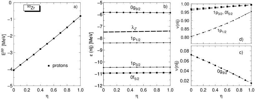
Figure 2: a) E_pp versus the $\eta$ parameter for the nucleus ⁹⁰Zr. b) Particle energies $\varepsilon$ in the canonical basis and c), d) occupation numbers $\nu(nlj)$ versus the $\eta$ parameter for the nucleus ⁹⁰Zr.

In fig. 2b) we present the proton single–particle energies, $\varepsilon{(nlj)}$, outside the Z$=28$ shell closure in the canonical basis, and in fig. 2c),d) the occupation $\nu(nlj)$ for each level $(nlj)$, which is given by

$$\nu(nlj)=\frac{1}{2j+1}\sum_{m}\langle\Phi|c_{nljm}^{\dagger}c_{nljm}|\Phi\rangle$$ (18)

In this figure we observe that the single–particle energies $\varepsilon$ barely change with $\eta$. With respect to the occupation numbers, we observe that the Coulomb pairing contribution goes in the direction to fill up the levels $0f_{5/2}$, $1p_{3/2}$ and $1p_{1/2}$ and to empty the level $0g_{9/2}$. That means, the Coulomb pairing term tries to increase the occupancy of the levels below the Fermi level at the cost of decreasing the occupancy of the levels above.

In the forth section of Table 1 we show the two–proton separation energies $S^{2p}(N,Z)=E(N,Z-2)-E(N,Z)$. As we can see in the table we obtain similar results in all approximations and the agreement with the experiment is good in all cases. We can understand this result if we consider that the binding energies are well described in all approximations and that that $S^{2p}$ is not an observable related with the pairing properties of the nuclei, which are really sensitive to the different approximations.

Finally, to complete the study of the neglected terms we shall now investigate the contributions of the spin-orbit term and of the two-body correction of the kinetic energy to the pairing field. In the fifth section of Table 1 we show the binding energies $E_{so,tk}$ obtained by adding these terms at the end of the minimization of eq. (15), i.e.,

$$E_{so,tk}=E_{HFP}+[V^{P}_{SO}+V^{P}_{TK}]$$ (19)

in a similar notation as introduced above. These terms are repulsive and a few hundred keV large. If these two terms are now taken into account selfconsistently we obtain the exact solution, i.e., HFB_e, of the full HFB equations, eq. (8). The resulting energies are on the average 100 keV smaller than if the terms are considered perturbationally. The last two entries of the table are the pairing energies $E^{pp}_{so,tk}$, defined as before. We observe that these terms provide an additional quenching of the pairing correlations. The behavior is similar to the one observed with the other terms, i.e., the largest quenching takes place for the semi-magical nucleus ⁹⁰Zr. For this particular nucleus we have calculated the effect of taking into account selfconsistently only one term and the other one perturbationally, i.e., we have performed the following calculations

$$E_{SO,tk}=E_{HFP}+V^{P}_{SO}+[V^{P}_{TK}]$$ (20)

$$E_{so,TK}=E_{HFP}+V^{P}_{TK}+[V^{P}_{SO}].$$ (21)

We obtain $E^{pp}_{SO,tk}=-1.671$ MeV, $E_{SO,tk}=-784.360$ MeV and $E^{pp}_{so,TK}=-1.355$ MeV, $E_{so,TK}=-784.354$ MeV, here again capital letters mean selfconsistent and small letters perturbational approaches. As we can see each term provides about half of the total effect.

3.2 The N$=82$ and N$=126$ regions

In this section we focus on the chains of the N$=82$ and N$=126$ isotones, again with neutron shell closure. Then, only proton pairing correlations are going to be important in this region. Two approximations are used in this case: the approximation HFB_s, see eq. (10), which neglects all the terms mentioned in the introduction, and the exact calculation HFB_e, see eq. (8), which takes into account all the contributions from the different terms of the force to the fields. In the HFB_s approximation, the missing terms are not added at the end of the variational procedure. In order to be able to compare the total binding energies in the HFB_s approach with the exact ones one must add these terms perturbativaly, i.e, the HFB_s+ approximation. In the N$=82$ region, the basis is determined by $q=1.0$, $p=1.0$ and $N_{0}=11.1$ and in this case the parameterization D1 is used. In the N$=126$ region, the basis $q=1.0$, $p=1.0$ and $N_{0}=12.1$ has been used and for the force parameterization we have chosen D1S.

In the first two columns of Table 2 we display the total binding energies. We find that the approach HFB_s+ provides a very good approximation to the exact results. In the last three columns of the same table we show the proton–proton pairing energies obtained in the approximations HFB_s, HFB_s+ and the exact ones HFB_e. Both approximations provide more proton pairing correlations that the exact calculation HFB_e. We can see that, contrary to the total binding energy case, the perturbational calculation HFB_s+ is not a good approximation for the pairing energy. We do not find any noticeable difference between both mass regions or the Gogny parameterizations.

From these results we may conclude that, for spherical nuclei, the approximation of ignoring some terms of the hamiltonian, HFB_s, presents some differences with the exact calculation. The approximation of considering these terms at least in first order perturbation theory, HFB_s+, works well for observables related to, or that can be obtained from, total binding energies. On the other hand, the wave function content may be different from the one obtained in the exact calculation.

Nucleus	Es+	Ee	E${}^{pp}_{s}$	E${}^{pp}_{s+}$	E${}^{pp}_{e}$
${}_{50}^{132}$Sn	-1090.875	-1090.891	-0.0000	-0.0000	-0.0000
${}_{52}^{134}$Te	-1111.079	-1111.236	-7.4700	-6.5881	-4.7615
${}_{54}^{136}$Xe	-1129.549	-1129.784	-11.7377	-10.3805	-7.4571
${}_{56}^{138}$Ba	-1146.233	-1146.557	-14.3629	-12.7469	-8.6469
${}_{58}^{140}$Ce	-1161.102	-1161.511	-15.7718	-14.0409	-8.8442
${}_{80}^{206}$Hg	-1615.860	-1616.038	-6.6570	-5.8068	-4.2799
${}_{82}^{208}$Pb	-1634.620	-1634.639	-0.0000	-0.0000	-0.0000
${}_{84}^{210}$Po	-1642.746	-1642.885	-6.1489	-5.3940	-3.9841
${}_{86}^{212}$Rn	-1649.656	-1649.878	-10.5256	-9.2758	-6.6871
${}_{88}^{214}$Ra	-1655.273	-1655.560	-13.7754	-12.1942	-8.2135

Table 2: Binding energies and proton pairing energies (in [MeV]) for spherical $N=82$ and $N=126$ nuclei with the methods HFB_s and HFB_e for $I=0\hbar$.

4 Normal deformed nuclei

In this section we will study the effects neglecting some terms in the hamiltonian for deformed nuclei. In particular we shall investigate their behavior at high angular momentum as well as the impact of the exchange terms on the neutron system.

4.1 Rare earth nuclei

In this region, we study six nuclei: the three Erbium isotopes ^164,166,168Er, and the three Ytterbium isotopes, ^162,164,166Yb. As in the preceding subsection we shall investigate only the approximation HFB_s (or HFB_s+ when the last one does not make sense) to compare with the exact calculation HFB_e and the experimental results when available. For these calculations we use the basis with q$=1.3$, p$=1.0$ and N${}_{0}=11.1$ and the D1S parameterization of the force.

	164Er	166Er	168Er	162Yb	164Yb	166Yb
Es+	-1328.665	-1343.424	-1357.391	-1305.810	-1322.764	-1339.332
Ee	-1329.176	-1343.868	-1357.777	-1306.361	-1323.425	-1340.123
E${}^{pp,\pi}_{s}$	-7.068	-6.297	-5.642	-10.081	-9.354	-8.309
E${}^{pp,\pi}_{e}$	-1.723	-1.727	-1.730	-4.167	-0.001	-0.000
E${}^{pp,\nu}_{s}$	-8.757	-7.475	-5.602	-9.444	-9.449	-9.049
E${}^{pp,\nu}_{e}$	-7.756	-6.310	-4.310	-8.223	-11.005	-9.614
Qs	7.590	7.781	7.893	6.073	6.871	7.563
Qe	7.552	7.712	7.836	6.190	7.602	7.787

Table 3: Ground state binding energies, pairing energies (in [MeV]), and quadrupole momenta (in barns), and in the approximation (HFB_s) and in the exact one (HFB_e).

We shall first investigate the ground state properties of these nuclei. In the upper part of Table 3 we show the binding energies. We find that the approximate calculation, HFB_s+, provides results very close to the exact ones. In the middle of the table we display the pairing energies calculated in both approaches. We find that the exact calculation provides proton pairing energies much smaller, in absolute value, than the approximate calculation, HFB_s. The global effect that we observe in the HFB_e calculations is a decrease of the absolute value of the proton pairing correlations compared to the approximate calculation. For ¹⁶⁴Yb and ¹⁶⁶Yb these correlations even vanish. The behavior of the neutron pairing energy is different depending on the nucleus: for the last two nuclei $|E^{pp,\nu}_{e}|$ is increased by about $1$ MeV and for the other nuclei it is decreased by approximately the same amount as compared to $|E^{pp,\nu}_{s}|$. In general, we can say that the global effect of including the Coulomb exchange and pairing contributions in the self–consistent procedure is a strong reduction of the absolute value of the proton pairing correlations in all the cases. The circumstance that the inclusion of the neglected terms influences more the proton pairing than the neutron one is obviously due to the Coulomb terms that do not affect the neutron system. With respect to the quadrupole moments we observe that the relative variation between both calculations is relative small, approximately $0.5\%$ for all the nuclei except for ¹⁶⁴Yb where Q increases in the exact calculation by about $10\%$.

The fact that the total binding energies are very close in both approaches is the reason why the non self–consistent and perturbational approximation has been considered in the past as a good approximation in spite of the fact that the wave functions are different.

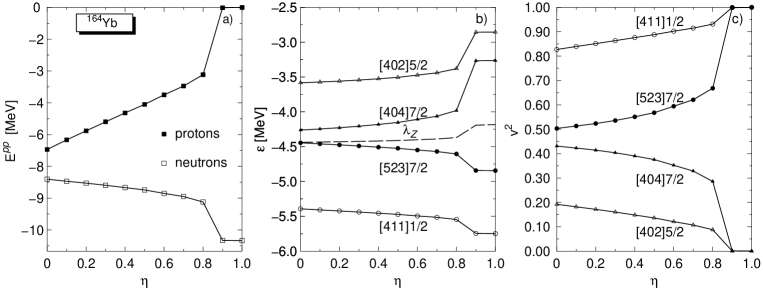
Figure 3: a) Variation of the pairing energies versus the $\eta$ parameter for the nucleus ¹⁶⁴Yb. b) Proton single particle energies $\varepsilon$ (in MeV). The Fermi level is the dashed line. c) Occupations $v^{2}$ of the levels in the canonical basis, versus the $\eta$ parameter, for the nucleus ¹⁶⁴Yb. The levels have been labeled by the quantum numbers $[n\,n_{z}\,l_{z}]\Omega$ in an axial basis.

The proton pairing energies of the nuclei ¹⁶⁴Yb and ¹⁶⁶Yb show an anomalous behavior: For these nuclei, the proton pairing correlations vanish completely in the HFB_e approach. Taking into account the behavior of the Er isotopes in Table 3, it would be expected to obtain for the nuclei ¹⁶⁴Yb and ¹⁶⁶Yb approximately $-4$ MeV for the proton pairing energy. In order to understand this quenching we have performed a calculation for ¹⁶⁴Yb similar to the one done for the nucleus ⁹⁰Zr switching off progressively the Coulomb pairing contribution. In Fig. 3a) the proton and neutron pairing energies are displayed versus the $\eta$ parameter. As it can be seen from this figure, increasing the $\eta$ value up to $\eta=0.8$ produces a linear increase of the proton pairing energy. However, for $\eta=0.9$ a sharp increase is obtained, going to the unpaired solution. By extrapolation of the small $\eta$ values to $\eta=1.0$ the expected proton pairing energy for this value would be around $-2.5$ MeV. However, the selfconsistent solution at $\eta=1.0$ corresponds to a non-paired proton system, which seems to indicate that the mean field approximation breaks down collapsing to the non-correlated regime. In Fig. 3b) we show the proton single particle energies in the canonical basis versus the $\eta$ parameter. Here we can observe the effect of the sharp phase transition on the single particle energies. In Fig. 3c) we can see how the occupations of the levels above (below) the Fermi level get empty (full). This sharp phase transition will explain the anomalous behavior of these two nuclei. The phase transition itself has more to do with the mean field approach than with the exchange terms. This can be seen very clearly in Fig.4a) where we show potential energy curves as a function of the proton fluctuation for different $\eta$ values. That means we have solved the HFB equations with an additional constraint on the w.f., namely the fluctuation in the proton number. For ¹⁶⁴Yb and $\eta=0$ we find a well defined minimum around the superfluid solution, $\langle(\Delta N)^{2}\rangle_{\pi}=5$, i.e., the mean field approach makes sense. For $\eta=0.9$, however, the energy surface is quite flat indicating that a theory able to include further correlations would be more appropriate. For ¹⁶²Yb, where no pairing collapse takes place, we find well defined minima for all $\eta$ values, see fig. 4b).

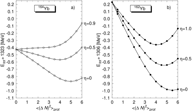
Figure 4: Binding energy versus the constrained proton fluctuation for different $\eta$ values.

Nucleus	$E_{\gamma}$ (EXP)	$E_{\gamma}$ (HFBs)	$E_{\gamma}$ (HFB${}_{s}+$)	$E_{\gamma}$ (HFBe)	$\Delta E_{\gamma}(\%)$
164Er	91.4	82.8	67.7	68.4	21.1
166Er	80.6	77.6	63.5	65.0	19.4
168Er	79.8	73.0	59.4	60.7	20.3
162Yb	166.9	115.7	90.3	93.9	23.2
164Yb	123.4	98.7	85.5	80.8	22.2
166Yb	102.4	88.8	75.9	75.8	17.2

Table 4: Experimental (¹⁶²Yb [14], ¹⁶⁴Er and ¹⁶⁴Yb [15], ¹⁶⁶Er and ¹⁶⁶Yb [16] and ¹⁶⁸Er [17]) and theoretical transition energies from $I=2\hbar$ to $I=0\hbar$ obtained with the methods HFB_s, the perturbational one HFB_s+, the exact calculation HFB_e (in keV) and the relative variation between HFB_s and HFB_e ($\%$).

In order to investigate the high spin properties of these nuclei we have solved the cranking HFB equations, eq. (2), in both approximations for the same nuclei. In Fig. 5, we display the pairing energies, $-E^{pp}$, as a function of the angular momentum. We find large differences between the approximate and the exact results. The absolute values of the HFB_s proton pairing energies are much larger than the exact ones, the difference being not only quantitative but also qualitative for the nuclei ¹⁶⁴Yb and ¹⁶⁶Yb. These nuclei remain super-fluid for the whole spin range in the approximate solution and normal fluid in the exact one. For the neutron system, the behavior is qualitatively similar in both approaches, the small differences observed depend on the nucleus considered. The strong quenching of the pairing energies obtained in the exact calculations will affect some observables, for example, the transition energies along the yrast band. In Table 4 we show the E${}_{\gamma}(2^{+}\longrightarrow 0^{+})$ values obtained in the approximations HFB_s, HFB_s+ and in the exact calculation. As it can be observed, to consider the exchange Coulomb term and all the contributions to the pairing field leads to a decrease in the transition energies, with a relative change around $20\%$. Since the perturbational calculation up to first order (HFB_s+) provides a good approximation to the total binding energies we expect that the transition energies calculated in this way will also be close to the exact ones. As we can see in the table this is the case. On the other hand, by comparing our results with the experimental ones, which are included in the same table, we observe that the HFB_e method gives a worse agreement with the experiment than the HFB_s+ one.

Figure 5: E^pp[MeV] versus angular momentum calculated with HFB_s (full symbols), HFB_e (empty symbols). The circles (boxes ) are for protons (neutrons).

It is interesting to know what happens with the D1 parameterization of the Gogny force. We have done the calculation with this parameterization for the nucleus ¹⁶⁴Er, we obtain the value $E_{\gamma}=95.7$ keV with HFB_s and $E_{\gamma}=79.0$ keV with HFB_e, with a relative variation between both calculations of $21.1\,\%$, the same relative variation as obtained with the D1S parameterization, as we can see in the Table 4. The two values of the transition energy E_γ obtained with the D1 are closer to the experiment, but again the approximate calculation HFB_s gives the best agreement with the experiment.

Figure 6: E_γ[MeV] versus angular momentum calculated with HFB_s (full circles), HFB_e (empty) and the experimental values (full squares). The empty squares in the panels of the nuclei ¹⁶⁴Er, ¹⁶⁸Er and ¹⁶⁴Yb represent the HFB_s+ approach. The experimental values are from: ¹⁶²Yb [14], ¹⁶⁴Er and ¹⁶⁴Yb [15], ¹⁶⁶Er and ¹⁶⁶Yb [16] and ¹⁶⁸Er [17].

The behavior of the gamma ray energies at high spin is displayed in Fig. 6 for the six analyzed nuclei, together with the experimental data. We find that the results of the approximation HFB_s are rather different from the exact ones as one expects from the disparity of the pairing energies found in the two calculations. For the nuclei ¹⁶⁴Er, ¹⁶⁸Er and ¹⁶⁴Yb we have also included the approximation HFB_s+. As expected the agreement with the exact calculation is much better than the one obtained in the HFB_s calculation. We have also checked the Slater approximation for deformed nuclei and at high angular momentum. That means, we have evaluated the Fock exchange Coulomb term in the Slater approximation and added it to the energy $E_{s}$ of eq. (10) before the variation. The results of these calculations, quadrupole moments, pairing energies and gamma ray energies along the Yrast band, practically coincide with the results of the plain HFB_s calculation.

Figure 7: The $\beta$ deformation parameter versus the angular momentum calculated with HFB_s (full symbols), HFB_e (empty symbols).

From the results discussed up to now, it seems that it is enough to consider the neglected terms in first order perturbation theory. This, however is not quite true since some observables can not be expressed as a function of the binding energies. For instance, the transition probabilities, magnetic moments, nuclear radii, etc. It is interesting to investigate the predictions for some of these observables in the exact and in the approximated calculation. In Fig. 7, we show the beta deformations as a function of the angular momentum for the six nuclei under study. The beta deformation parameter is mainly affected by the alignment effects and the pairing correlations. In general, larger pairing correlations imply smaller deformations and larger alignments smaller $\beta$-deformations (Coriolis anti-stretching effect). In the exact calculations, in general, we have smaller absolute values of the pairing correlations and larger alignment. In principle, one could expect a compensation and only in cases where one of the effects is much larger than the other one we should obtain a change in deformation corresponding to the largest effect. In the figure we observe that in the nuclei ¹⁶⁴Er, ¹⁶⁸Er and ¹⁶²Yb such a compensation takes place. In ¹⁶⁶Er the compensation takes place for small spins but not for large ones and in ¹⁶⁴Yb and ¹⁶⁶Yb there is no compensation at all. Looking in Fig. 6, we find that in ¹⁶⁶Er, there is clearly a stronger alignment in the exact solution than in the approximated one, which causes an smaller deformation in the exact calculation at high spins. In ¹⁶⁴Yb and ¹⁶⁶Yb the large quenching observed in the pairing energy explains the distinct behavior of the exact solution from the approximate one.

Figure 8: Reduced transition probabilities versus angular momentum calculated with HFB_s (full circles), HFB_e (empty) and the experimental ones (full squares). The experimental values are from ¹⁶²Yb [14], ¹⁶⁴Er and ¹⁶⁴Yb [15], ¹⁶⁶Er and ¹⁶⁶Yb [16] and ¹⁶⁸Er [17].

In Fig. 8 we present the reduced transition probabilities B(E2) for the nuclei we are analyzing. Though these probabilities are related with the $\beta$-deformations we expect larger differences between the two calculations in the B(E2) case because this quantity has to do only with protons while to the $\beta$-deformations both the proton and the neutron systems contribute. We should remember that neglecting the Coulomb exchange terms affects only the proton system. We find this supposition to be right, specially at high spins. For the nucleus ¹⁶⁴Yb there are differences even at zero angular momentum due to the change of deformation in the ground state (see Table 3). Though we find some differences between both calculation, in the comparison with the experimental results it does not matter which one we take.

Figure 9: Gyromagnetic factors versus angular momentum calculated with HFB_s (circles), HFB_e (squares). Full (empty) symbols are for protons (neutrons).

In Fig. 9 we finally present the gyromagnetic factors versus the angular momentum. For this observable we expect only small differences between the two calculations for the neutron gyromagnetic factor, $g_{n}$, for the same reasons as before, and somewhat larger for the proton gyromagnetic factor $g_{p}$. We find this supposition to be right. In the HFB_s approximation, the general behavior of these nuclei is, first, a more or less sharp neutron (i_13/2) alignment take place at medium spin values and then a proton (h_11/2) alignment take place at high spins. In the HFB_e calculation the situation is qualitatively similar with the exception of the nucleus ¹⁶⁶Er which shows a very delayed neutron alignment, contrary to the experimental situation [16].

4.2 Actinide region: The nucleus ²⁴⁰Pu.

In this subsection we shall now discuss an example of a heavy deformed nucleus, to see if there is a possible mass dependence of the terms neglected in the approximate calculations. As a representative of the actinide region we have chosen the nucleus ²⁴⁰Pu. In the calculations we have used the basis q$=1.3$, p$=1.0$ and N${}_{0}=14.0$ which is large enough to guarantee the convergence, and the D1S parameterization of the force. Let us first discuss the wave function content of the HFB_s approximation and of the exact theory HFB_e. In Fig. 10, panel (a), we show the pairing energies $E^{pp}$ in both theories as a function of the angular momentum. As before, we find a strong quenching for the values of the proton system in the HFB_e as compared to the HFB_s one. The values for the neutron system, on the contrary, are very similar in both approaches. In panel (b) we display the electric quadrupole moment. At small angular momentum both predictions are very close but at large angular momentum they differ by up to $2\%$ at the largest spin considered. The fact that the HFB_e prediction is smaller can be understood looking at panel (c) where we show the gyromagnetic factors. As expected the $g_{n}$ are very similar in both approaches for all spin values. The $g_{p}$, in the HFB_e prediction indicates a larger proton alignment than in the HFB_s one, which will cause the observed anti-stretching effect in the HFB_e approach.

Figure 10: Properties of the nucleus ²⁴⁰Pu along the yrast band in the HFB_s and HFB_e approaches. a) Pairing energies. b) Charge quadrupole moments. c)Gyromagnetic factors. d) Gamma ray energies. e) Moments of inertia ${\mathcal{J}}^{1}$ and f): Moments of inertia ${\mathcal{J}}^{(2)}$. The labels for panels a), b) and c) are the ones of panel c). The labels for d), e) and f) are listed in d). The experimental data are from [18].

With respect to observables related to energy differences, we can consider the approaches HFB_s, HFB_s+ and HFB_e. In the same figure, we present the transition energies $E_{\gamma}$, panel d), first moment of inertia ${\mathcal{J}}^{1}$, panel (e), and second moment of inertia ${\mathcal{J}}^{2}$, panel (f), in the three approaches, as well as the experimental data. The agreement of the plain HFB_s with the experiment for the three observables is spectacular. The exact solution HFB_e, according to the less pairing-correlated wave function, see panel (a), provides too large moments of inertia and too small gamma-ray energies. For the perturbative approach HFB_s+, we obtain values similar to the exact calculation HFB_e, though for the more sensitive quantity ${\mathcal{J}}^{2}$ some differences are found at the smallest and the largest angular momenta.

It is very remarkable that the HFB_s+ binding- and $\gamma$-ray energies are very close to the HFB_e ones. This fact also happens in the other nuclei calculated so far. To gain some insight in the reasons for this agreement we have calculated separately all contributions to the total energy in both approaches. That means, with the wave function $|\Phi\rangle_{s}$ determined by minimization of $E_{s}$, we have evaluated the Fock and pairing term of the Coulomb force, as well as the pairing terms stemming from the spin-orbit and the two-body kinetic energy terms. We have also separately calculated the mentioned terms with the wave function $|\Phi\rangle_{e}$ determined by minimization of the exact energy $E_{e}$. In the upper part of Table 5 we show the energy $E_{s}$ of Eq. (10) evaluated with the wave function $|\Phi\rangle_{s}$ (approach $s$) and with $|\Phi\rangle_{e}$ (approach $e$), as well as the terms just mentioned (we use the notation of Eq. (9)) for the ground state of ²⁴⁰Pu. The last column, denoted $E_{tot}$, corresponds to the total energy, $E_{s+}$ in the $s$ approach and $E_{e}$ in the $e$ one. As expected the binding energy is lower in the exact than in the perturbative calculation. On the other hand, since the wave function $|\Phi\rangle_{s}$ has been determined by minimizing $E_{s}$, it is also obvious that this quantity is lower in the $s$ approximation than in the $e$ one. Concerning the other terms, each of them separately provides a bigger energy lowering in the $e$ than in the $s$ appoach. We also observe that the relative largest difference between both approaches corresponds to the pairing Coulomb term. In the lower part of the same Table we show, as a function of the angular momentum, the energy differences $\Delta\xi=\xi(I)-\xi(I-2)$, where $\xi$ stands for each energy entry of the upper part of the Table, i.e., $\Delta\xi$ represents the contribution of each term to the gamma ray energy from the state $I$ to $I-2$. These energy differences have been calculated again in the approaches $s$ and $e$. Let us first concentrate on the $I=2\hbar$ row. The prediction for the gamma ray energy taking into account only the terms of the standard approach are almost identical independently of the fact that we evaluate them with $|\Phi\rangle_{s}$ or with $|\Phi\rangle_{e}$ and the same happens with the other terms. Obviously, if one adds all these contributions, the prediction for the total $\gamma$-ray energy with all terms is very similar in both approaches. It is also interesting to note that the contributions from the terms not considered in the standard approach are all negative and lead to a more compressed spectrum. We also observe that the largest contribution by far is the one from the Coulomb pairing term, though the other contributions are not at all negligible. At higher angular momentum we observe the same trend as for $I=2\hbar$, i.e., the energy differences for a given $I$ are very similar in both approaches. It seems therefore that the reason, for the good agreement of the gamma ray energies in both approaches, is that the dependence of the exchange terms from the angular momentum is almost identical in the HFB_s+ and in the HFB_e approaches. For $I=0\hbar$ the binding energies differ only by about 500 keV. The exchange terms are rather different in both approaches, however, when the $\gamma$-ray are calculated, the differences cancel and one gets similar values in both approaches.

$I$	App.	$E_{s}$	$V^{F}_{C}$	$V^{P}_{C}$	$V^{P}_{SO}$	$V^{P}_{TK}$	$E_{tot}$
0	$s$	-1766.259	-36.450	0.698	0.111	0.173	-1801.725
	$e$	-1765.862	-36.703	0.249	-0.007	0.091	-1802.232
		$\Delta E_{s}$	$\Delta V^{F}_{C}$	$\Delta V^{P}_{C}$	$\Delta V^{P}_{SO}$	$\Delta V^{P}_{TK}$	$\Delta E_{tot}$
2	$s$	42.5	-1.8	-4.5	-1.6	-1.7	32.9
	$e$	42.0	-1.5	-3.4	-2.7	-1.1	33.3
4	$s$	98.0	-4.7	-11.5	-4.2	-4.5	73.3
	$e$	99.1	-4.2	-9.4	-5.8	-2.6	77.1
6	$s$	152.0	-7.0	-17.4	-6.0	-6.5	114.8
	$e$	153.7	-6.8	-14.9	-8.6	-3.9	119.5
8	$s$	203.3	-9.5	-23.5	-8.0	-8.7	153.7
	$e$	207.8	-10.3	-22.2	-10.4	-5.2	159.7
10	$s$	250.8	-11.6	-28.9	-9.2	-10.0	190.9
	$e$	257.4	-14.0	-29.1	-11.4	-6.2	196.8
12	$s$	294.5	-14.6	-35.9	-10.5	-11.9	221.4
	$e$	306.1	-19.5	-38.8	-10.8	-7.0	229.9
14	$s$	333.7	-16.4	-40.9	-10.9	-12.6	252.8
	$e$	359.0	-29.7	-55.7	-8.3	-7.8	257.6

Table 5: Upper part: Ground state contributions to the binding energy of the nucleus ²⁴⁰Pu in the HFB_s+ and in the HFB_e approaches. The energies are given in MeV and the angular momenta in $\hbar$. Lower part: Contributions to the gamma ray energies along the Yrast band in keV in the HFB_s+ and in the HFB_e approaches.

5 Superdeformed nuclei in the A $\approx 190$ region

This region of superdeformation has already been studied using the HFB_s method with the Gogny force D1S [6, 7]. In our calculations we use the basis q$=1.5$, p$=1.0$ and N${}_{0}=12.5$ and the D1S interaction. Taking into account the results obtained in the other regions, we do not expect a big influence of the Coulomb exchange terms because for the superdeformed states the proton pairing energies either vanish or are very small even with the HFB_s method. A large change of the pairing energies due to the Coulomb exchange and the other terms cannot exist, therefore, in this states. As an example of superdeformation we have chosen the nucleus ¹⁹⁰Hg. From this example we will learn how the other pairing contributions (spin–orbit and two–body correction) affect the neutron pairing energies and the other nuclear properties through the selfconsistency. As before, we shall first look for the wave function content of the HFB_s and the HFB_e approaches. In Fig. 11, panel (a), we can see the behavior of the pairing energies in both methods. As mentioned, the proton pairing energies along the band vanish in both calculations. The neutron pairing energies are close to each other in both calculations, though somewhat smaller values are obtained for the HFB_e at low angular momentum. The charge quadrupole moment is depicted in panel (b). Only small differences between both approaches are found at large angular momentum. The gyromagnetic factors, panel (c), are again very close to each other. We shall now turn to a comparison between the HFB_s, HFB_s+ and HFB_e predictions for the $\gamma$-ray energies, panel (d), first moments of inertia, panel (e) and second moments of inertia, panel (f). For these observables we do not find remarkable differences between the three approaches.

Figure 11: Same as fig. 10 but for the nucleus ¹⁹⁰Hg. The experimental data are from ref.[19].

From this section we may conclude that the Coulomb exchange and pairing contribution barely modify the properties of the nucleus when the approximate calculation HFB_s has vanishing proton pairing energies. Then, the approach HFB_s is a good approximation to the completely self–consistent calculation, HFB_e, even for the wave function.

6 Energy Surfaces

In this section we shall finally investigate the effect of the exchange terms as a function of a collective variable at zero angular momentum. We have used an axially symmetric HFB code that allows reflexion asymmetric shapes. We have performed two different calculation. In the first one we have neglected all exchange terms, i.e., the HFB_s approach, but we have included, the Fock Coulomb term in the Slater approximation, we shall call this approach HFB_s,Sla. The second approach includes all exchange terms with the exception of the contribution of the spin-orbit term to the pairing field, we shall call this approach HFB_e,nso. Notice that since we do not add at the end of the calculation HFB_s,Sla the pairing terms of the Coulomb and the two-body kinetic energy (both contributions are repulsive) it is possible to find HFB_s,Sla solutions with an energy deeper than the HFB_e,nso approach. That means we are more interested in the general behavior of the energy surface than in the absolute values. The most common case of energy dependence as a function of a collective variable appears in the calculation of fission barriers. In this calculations we use the basis q$=1.5$, p$=1.0$ and N${}_{0}=15.1$ and the D1S parameterization. In fig. 12, on panel a), we display the binding energy of ²⁵⁴No as a function of the constrained quadrupole moment in both approaches. We find a similar behavior in both calculations, though small differences are noticeable. For example, the height of the first barrier is slightly larger in the HFB_e,nso approach than in the HFB_s,Sla. The second one, however, has more or less the same height in both approaches. In panel b) we display the pairing energies along the fission path. The neutron pairing energy is practically the same in both calculations. The proton pairing energies in the HFB_e,nso calculations show the Coulomb antipairing effect already discussed in other nuclei. They are in absolute value 5 to 10 MeV smaller than in the calculation without Coulomb pairing term.

Figure 12: a) Results in the HFB_s,Sla approach, crosses, and HFB_e,nso, filled circles. a) Binding energy of the nucleus ²⁵⁴No versus the quadrupole moment. b) Pairing energies along the fission barrier, protons (neutrons), dashed (solid) line. c) Binding energy of the nucleus ²²⁶Th versus the octupole moment. d) Dipole moment versus the octupole moment.

We shall now investigate the effect of the exchange terms in cases where the reflexion symmetry is broken i.e. the wave functions do not have a good parity. In these calculations we use the same theoretical approaches as in the ²⁵⁴No ones, we use the basis q$=1.3$, p$=1.0$ and N${}_{0}=13.1$ and the D1S interaction. In panel c) of the same figure, we present the binding energy of the nucleus ²²⁶Th versus the constrained octupole moment. As with the quadrupole operator we do not find any remarkable difference between both calculations. The depth and shape of the octupole deformed minimum are almost identical in both approaches. In panel d), finally, we present the dipole moment versus the constrained octupole momentum. Again, small differences between both calculations are found but without further relevance.

7 Discussion

The main outcome of our investigation is that the exchange terms usually neglected affect mainly the nuclear pairing properties. More specifically, they affect mostly the proton nuclear pairing properties because of all missing terms the largest contribution to the pairing field arises from the Coulomb potential. Observables little or not dependent on the pairing correlations, are, therefore, not affected by these terms. On the contrary, observables like the moments of inertia or two-quasiparticle states energies, strongly dependent on pairing correlations, are very sensitive to these terms.

We have found that the results of calculations performed with the plain HFB_s approximation differ significantly, for some observables, from those of the exact solution HFB_e, in nuclei where the proton pairing energies are relatively large. On the contrary, the HFB_s+ results agree, in general, very well with those of the exact solution. In cases of very small proton correlation energies all three approaches, HFB_s, HFB_s+ and HFB_e practically coincide.

For those situations where proton correlations are relevant, the predictions of the HFB_s approximation agree better with the experimental data than the exact ones or than the ones from the HFB_s+ approximation. Paradoxically, the Gogny force was fitted [2] using the exact HFB approach to calculate properties of spherical nuclei. The pairing properties of the Gogny force were adjusted by fitting the odd-even mass difference of the $Sn$ isotones. The $Sn$ isotones, however, have a major shell closure in protons, Z$=50$, and in this case, practically, it does not matter whether one performs approximate or exact calculations, i.e., effectively the Coulomb exchange terms were not considered in this fit. Furthermore, the fact that including the exchange terms in the calculations worsens the good agreement of the theoretical results with the experimental data, reinforces the conjecture that the actual fits of the Gogny force should be used, in calculations with open proton shells, without the mentioned terms.

Of course the Gogny force is isospin invariant but the Coulomb force is not. The Hartree-Fock potential that one obtains after solving the HFB equations neither is isospin invariant. It is not clear, therefore, that a different parameterization (concerning the pairing part of the interaction) of the force would not be obtained if nuclei with open proton shells had been considered in the fit. The whole issue of adjusting the pairing properties of any force is itself rather fuzzy. Most of the fits have been done to reproduce the experimentally observed odd-even mass difference. This energy difference can, however, not be attributed only to pairing correlations [20]. From the theoretical point of view the calculation of this energy difference presents also problems because binding energies of odd nuclei are not easy to calculate. Blocking effects and angular momentum projection should be performed in order to evaluate properly this energy, besides additional couplings. However, in order to save CPU time during the fit, approximations are used, in particular in order not to break the time reversal symmetry the equal filling approximation is used.

Taking into account the complication of the neglected exchange terms, see Appendix B, the fact that the HFB_s approximation, commonly used in most HFB calculations, provides such good agreement with the experimental data is very fortunate.

8 Conclusions

For the first time we have performed an exact self–consistent HFB calculation in a triaxial basis with the Gogny force. The exact Coulomb exchange term and the contributions of the spin–orbit, two–body correction of the kinetic energy and Coulomb terms to the pairing field have been included in the calculations. An exhaustive analysis of each term has been performed for spherical nuclei in different mass regions. We find the Coulomb contribution to the pairing field to be the most relevant one. The other terms, though not negligible, give smaller contributions.

For deformed nuclei we have studied the commonly used HFB_s approximation, the perturbative HFB_s+, and the exact solution. We have been concerned with different mass regions at zero and high spins. As in the case of spherical nuclei, we observe a reduction of the proton pairing energies in the exact calculations as compared to the HFB_s ones. Ground state energies are very similar in the perturbative and in the exact calculations. Energies of excited states are somewhat different in the HFB_s approximation than in the exact one. We have also investigated superdeformed states. Since the proton pairing correlations of these nuclei are small we do not find any significant difference between the approximate and the exact solution. Lastly, we have analyzed the effect of the most relevant exchange terms in the calculation of energy surfaces. The energy as a function of the quadrupole (octupole) mass operator is practically identical in the approximate and in the exact calculations.

We also have found, that the Slater approximation for the Fock Coulomb term is a good one for all HFB calculations, in agreement with ref.[3] for the HF case.

For all nuclei and situations analyzed the following general conclusions apply:

1. In cases where the proton pairing correlations do not play an important role, anyone of the approximations considered practically coincide with the exact calculation.

2. When proton pairing correlations are relevant, then:

   • For energy-related observables the perturbative approach HFB_s+ is a good approximation to the exact one.

   • For those observables whose evaluation requires the wave functions, one should perform the exact calculation.

   • If the HFB wave functions are thought as a basis for more elaborated theories, like RPA or GCM, then the exact calculation is required.

3. The way in which the fits of the Gogny force were performed favors neglecting the mentioned exchange terms in HFB calculations using these fitted parameter sets.

It remains to investigate the real importance of this terms by performing new fits of the Gogny force taking into account explicitly all terms discussed here.

We thank J.F. Berger, M. Girod and S. Peru for discussions. This work was supported in part by DGICyT, Spain under Project PB97-0023. One of us (M.A) acknowledges a grant from the Spanish Ministery of Education under Project PB94-0164.

Appendix A: The interaction

As an effective interaction we use the Gogny force [2]

$$v_{12} = \sum_{i=1}^{2}e^{-{(\vec{r}_{1}-\vec{r}_{2})}^{2}/\mu_{i}^{2}}(W_{i}+B_{i}P_{\sigma}-H_{i}P_{\tau}-M_{i}P_{\sigma}P_{\tau})+$$ (22)

$$+ W_{LS}(\vec{\sigma}_{1}+\vec{\sigma}_{2})\vec{k}\times\delta(\vec{r}_{1}-\vec{r}_{2})\vec{k}+$$

$$+ t_{3}(1+x_{0}P_{\sigma})\delta(\vec{r}_{1}-\vec{r}_{2})\rho^{1/3}\left(\frac{1}{2}(\vec{r}_{1}+\vec{r}_{2})\right),$$

and the Coulomb force

$$v_{12}^{C}=(1+2\tau_{1z})(1+2\tau_{2z})\frac{e^{2}}{|\vec{r}_{1}-\vec{r}_{2}|}.$$ (23)

Additional contributions taken into account in the calculations arise from the one–body and two–body center of mass corrections

$$\hat{T}=\sum_{i}\frac{{\vec{p}_{i}}^{\,2}}{2m}\left(1-\frac{1}{A}\right)-\frac{1}{Am}\sum_{i>j}\,\vec{p}_{i}\cdot\vec{p}_{j}.$$ (24)

In the calculations we use the parametrizations D1S [8] and D1 [2, 9].

Appendix B: Calculation of the Coulomb Hartree-Fock field and pairing tensor.

To compute the Hartree-Fock field and pairing tensor for the Coulomb interaction we have followed the idea used in [4]. It amounts to use the identity

$$\frac{1}{|\vec{r}_{1}-\vec{r}_{2}|}=\frac{2}{\sqrt{\pi}}\int_{0}^{\infty}\frac{d\mu}{\mu^{2}}e^{-\left(\vec{r}_{1}-\vec{r}_{2}\right)^{2}/\mu^{2}},$$

to compute the Coulomb matrix elements in terms of those of Gaussians with range $\mu$. The main advantage of this approach is that the matrix elements of the Gaussians are factorizable in terms of quantities defined for each Cartesian direction $x$, $y$ and $z$. Unfortunately, the price to pay is the $\mu$ integration. Introducing the HF field $\Gamma^{G}_{k_{1}k_{2}}(\mu)$ and the pairing tensor $\Delta^{G}_{k_{1}k_{2}}(\mu)$, see eq.(6), of a Gaussian of range $\mu$ we can express the corresponding quantities for the Coulomb potential as

$$\Gamma^{C}_{k_{1}k_{2}}=\frac{2e^{2}}{\sqrt{\pi}}\int_{0}^{\infty}\frac{d\mu}{\mu^{2}}\Gamma^{G}_{k_{1}k_{2}}(\mu)$$

and

$$\Delta^{C}_{k_{1}k_{2}}=\frac{2e^{2}}{\sqrt{\pi}}\int_{0}^{\infty}\frac{d\mu}{\mu^{2}}\Delta^{G}_{k_{1}k_{2}}(\mu)$$

To transform the integration interval to a finite one, one makes the change of variables $u^{2}=\left(1+\alpha\mu^{2}\right)^{-1}$, with $\alpha$ a parameter to be determined below. We finally obtain

$$\Gamma^{C}_{k_{1}k_{2}}=2e^{2}\sqrt{\frac{\alpha}{\pi}}\int_{0}^{1}\frac{du}{\left(1-u^{2}\right)^{3/2}}\Gamma^{G}_{k_{1}k_{2}}\left(\frac{\sqrt{\frac{1}{\alpha}\left(1-u^{2}\right)}}{u}\right)$$

and

$$\Delta^{C}_{k_{1}k_{2}}=2e^{2}\sqrt{\frac{\alpha}{\pi}}\int_{0}^{1}\frac{du}{\left(1-u^{2}\right)^{3/2}}\Delta^{G}_{k_{1}k_{2}}\left(\frac{\sqrt{\frac{1}{\alpha}\left(1-u^{2}\right)}}{u}\right).$$

The integrations are carried out numerically with the Gauss-Legendre method. The optimal choice of $\alpha$, turns out to be equal to the maximum of $\left(\alpha_{x},\alpha_{y},\alpha_{z}\right)$ where $\alpha_{i}=\frac{1}{2b_{i}^{2}}$ and $b_{i}$ are the oscillator lengths (see ref. [4]).

In the numerical computation of the Coulomb exchange and pairing terms we have used 20 points for the Gauss-Legendre integration. This number of points has proven to be enough for a precise determination of the exchange field and pairing tensor. The number of integration points used makes the evaluation of the Coulomb terms rather costly in terms of CPU time: it usually takes a factor 5.5 longer to compute those factors than to calculate the Fock and pairing parts of the Brink-Boecker interaction (in this case, we have two gaussians and we have to compute them for both protons and neutrons). The calculation of the exchange and pairing parts of the BB interaction is already the most costly part of each iteration as it usually takes between a factor 10 and 15 longer than the evaluation of the direct terms. In a standard workstation and for a configuration space with parameters $p=1$, $q=1.3$ and $N_{0}=11.1$ the evaluation of the direct field takes 1.9 seconds, the combined Fock and pairing terms of the BB part takes 19 seconds and the evaluation of the Fock and pairing parts of the Coulomb interaction takes 103 seconds. One has to keep in mind that the previous numbers are for each iteration of the minimization process. If we increase the size of the basis by using $q=1.6$ and $N_{0}=14.0$ the previous numbers climb up to 7, 92 and 540 seconds respectively. We clearly see the tremendous slow down introduced in the calculations stemming from the consideration of the Fock and pairing terms of the Coulomb interaction. This tremendous slow down can be even worse for the practitioners of the Skyrme interaction as their CPU time consumption per iteration has to be of the order of the one needed to calculate the direct field of the Gogny force.

Concerning the computation of the pairing field associated to the spin-orbit interaction we have followed the ideas already presented in [4]. An explicit expression for all these terms can be found in [21]. The numerical computation of this field takes almost the same time as the computation of the HF field and therefore, its inclusion is not significant in terms of CPU time.

References

- [1] D. Vautherin and D.M. Brink, Phys. Rev. C 5 (1972), 626.
- [2] J. Dechargé and D. Gogny, Phys. Rev. C 21 (1980), 1568.
- [3] C. Tintin-Schnaider, Ph. Quentin, Phys. Lett. 49B (1974), 397.
- [4] M. Girod and B. Grammaticos, Phys. Rev. C 27 (1983), 2317.
- [5] J.L. Egido and L.M. Robledo, Phys. Rev. Lett 70 (1993), 2876.
- [6] M. Girod, J.P. Delaroche, J.F. Berger, Phys. Lett. 325B (1994), 1.
- [7] A. Valor, J. L. Egido and L.M. Robledo, Nucl. Phys., A665 (2000) 46-70.
- [8] J.F. Berger, M. Girod and D. Gogny, Comp. Phys. Comm. 63 (1991), 365.
- [9] D. Gogny, Nuclear selfconsistent fields. Eds. G. Ripka and M. Porneuf (North Holland 1975).
- [10] J.L. Egido and L.M. Robledo, Nucl. Phys. A570 (1994), 69c.
- [11] P. Ring and P. Shuck, The Nuclear Many Body Problem (Springer-Verlag, Berlin, 1980).
- [12] J.L. Egido, J. Lessing, V. Martin and L.M. Robledo, Nucl. Phys. A594 (1995), 70.
- [13] G. Audi and A. H. Wapstra, Nucl. Phys. A565 (1993), 1.
- [14] R.G. Helmer, Nuclear Data Sheets 64 (1991), 79.
- [15] E.N. Shurshikov and N.V. Timofeeva, Nuclear Data Sheets 65 (1992), 365.
- [16] E.N. Shurshikov and N.V. Timofeeva, Nuclear Data Sheets 67 (1992), 45.
- [17] V.S. Shirley, Nuclear Data Sheets 71 (1994), 261.
- [18] E.N. Shurshikov and N.V. Timofeeva, Nuclear Data Sheets 59 (1990), 947.
- [19] B. Crowell et al., Phys.Rev. C51, R1599 (1995).
- [20] J. Dobaczewski, P. Magierski, W. Nazarewicz, W. Satula and Z. Szymanski, arXiv:nucl-th/0003019.
- [21] M. Anguiano, Ph. D. Thesis, Universidad Autonoma de Madrid, 2000, unpublished.