Spatially inhomogeneous condensate in asymmetric nuclear matter

Abstract

We study the isospin singlet pairing in asymmetric nuclear matter with nonzero total momentum of the condensate Cooper pairs. The quasiparticle excitation spectrum is fourfold split compared to the usual BCS spectrum of the symmetric, homogeneous matter. A twofold splitting of the spectrum into separate branches is due to the finite momentum of the condensate, the isospin asymmetry, or the finite quasiparticle lifetime. The coupling of the isospin singlet and triplet paired states leads to further twofold splitting of each of these branches. We solve the gap equation numerically in the isospin singlet channel in the case where the pairing in the isospin triplet channel is neglected and find nontrivial solutions with finite total momentum of the pairs. The corresponding phase assumes a periodic spatial structure which carries a isospin density wave at constant total number of particles. The phase transition from the BCS to the inhomogeneous superconducting phase is found to be first order and occurs when the density asymmetry is increased above 0.25. The transition from the inhomogeneous superconducting to the unpaired normal state is second order. The maximal values of the critical total momentum (in units of the Fermi momentum) and the critical density asymmetry at which condensate disappears are $P_{c}/p_{F}=0.3$ and $\alpha_{c}=0.41$. The possible spatial forms of the ground state of the inhomogeneous superconducting phase are briefly discussed.

I Introduction

The theory of fermion pairing when the fermions, which are bound in Cooper pairs, lie on different Fermi surfaces was addressed in the early 1960s in the context of metallic superconducting alloys containing paramagnetic impurities[1, 2, 3, 4]. Recently, the theory has received renewed attention in several contexts, including the pairing in asymmetric nuclear matter[5, 6, 7, 8, 9, 10, 11] and color superconductivity in flavor-asymmetric high-density QCD[12, 13].

This paper elaborates on an earlier suggestion[8] that the ground state of the superconducting asymmetric nuclear matter at large asymmetries corresponds to a pair condensate with nonzero total momentum of the Cooper pairs. The argument is based on the observation by Larkin and Ovchinnikov[14] and Fulde and Ferrell [15] who first showed, in the context of the metallic superconductors, that the Bardeen-Cooper-Schrieffer (BCS) equations admit solutions with nonzero total momentum of Cooper pairs. In the configuration space such a condensate forms a periodic lattice with finite shear modulus. The resulting spatially inhomogeneous superconducting state is called the Larkin-Ovchinnikov-Fulde-Ferrell (LOFF) phase.

The occurrence of pair correlations crucially depends upon the overlap between the neutron and proton Fermi surfaces; the pairing gap is largest in the isospin symmetric case and is suppressed as the system is driven out of the symmetric state. The thermal smearing of the Fermi surfaces promotes the pairing, but, however is ineffective when the separation between the surfaces is large compared to the temperature. If the total momentum of the Cooper pairs is zero, the Fermi surfaces (for homogeneous systems) are located on concentric spheres. If, however, a Cooper pair moves with a finite momentum, the centers of the spheres are shifted. This allows for the pairing, even for vastly different radii of the spheres, since now the nonconcentric spheres may intersect. The overlap regions then provide the kinematical phase space for pairing phenomena to occur.

The microscopic calculations, based on the BCS theory for the bulk nuclear matter show that the isospin-symmetric matter supports Cooper-type pair correlations in the ${}^{3}S_{1}$-${}^{3}D_{1}$ partial-wave channel due to the tensor component of the nuclear force. The energy gap is of the order of 10 MeV at the empirical saturation density (Refs. [5, 6, 7, 8, 9, 10, 11] and references therein) if one assumes that the effective pairing interaction can be approximated by the bare interaction and if the renormalization of the single particle spectrum reduces the density of the state at the Fermi surface by a factor of 2.

There is little evidence for large gap isospin singlet pairing in ordinary nuclei[18], which is evidently suppressed due to the spin-orbit splitting[19]. The laboratory data do not exclude the possibility that the bulk nuclear matter, as encountered in the supernovas and neutron stars, may support large gap pairing in the isospin singlet channel. In the model of “nucleon stars”[20] the kaon condensation implies nearly isospin symmetric matter, in which case the isospin singlet pairing can play a major role in determining the cooling and rotation dynamics of such objects. Note, however, that in the models without meson condensates the proton concentration in supernova and neutron star matter is of the order of $5\%-30\%$ and these asymmetries are too large to allow for neutron-proton pairing. In the high-density regime, the hyperon-rich neutron star matter may be much more symmetric than at the densities around the saturation density[21] and therefore can support neutron-proton pairing, most likely due to the attractive ${}^{3}D_{2}$ partial-wave interaction[7]. If the nucleon-hyperon and hyperon-hyperon interactions are attractive, the pairing among fermions lying on different Fermi surfaces, and in particular the formation of the LOFF phase, could be a realistic possibility in hyperon rich matter. Finally, in superstrong magnetic fields of highly magnetized neutrons stars (magnetars) the Pauli paramagnetism will cause a splitting in the Fermi energies of the spin-up and spin-down fermions; in this case the pairing in the isospin triplet channel among the $S$-wave paired neutrons should exhibit the properties of the LOFF phase.

Before turning to the main body of the paper, we draw the reader’s attention to Ref. [16] who considered the color superconducting LOFF phase in the context of high-density QCD and Ref. [17] who considered the finite momentum pairing between quarks in the particle-hole channel (chiral condensate). Our work, to some extent, parallels the former reference, but we do not attempt any comparison at this stage, as the formalisms and contexts are entirely different.

In Sec. II we derive the BCS equations, which include the effects of the finite momentum of the Cooper pairs, within the finite temperature real-time Green’s functions formalism. The numerical solutions of these equations are shown in Sec. III. Sec. IV contains a summary of the results.

II Formalism

Below, we shall use the real-time Green’s functions extended to the Nambu-Gor’kov space to account for pair correlations. The single particle retarded Green’s function in this space is defined as usual:

$$i\hat{G}_{\alpha\beta}(x_{1},x_{2})\equiv i\left(\begin{array}[]{cc}G_{\alpha\beta}(x_{1},x_{2})&F_{\alpha\beta}(x_{1},x_{2})\\ F_{\alpha\beta}^{\dagger}(x_{1},x_{2})&G_{\alpha\beta}^{\dagger}(x_{1},x_{2})\end{array}\right)=\left(\begin{array}[]{cc}\left<T_{t}\psi_{\alpha}(x_{1})\psi_{\beta}^{\dagger}(x_{2})\right>&\left<T_{t}\psi_{\alpha}(x_{1})\psi_{\beta}(x_{2})\right>\\ \left<T_{t}\psi_{\alpha}^{\dagger}(x_{1})\psi_{\beta}^{\dagger}(x_{2})\right>&\left<T_{t}\psi^{\dagger}_{\beta}(x_{1})\psi_{\alpha}(x_{2})\right>\end{array}\right),$$ (5)

where $\alpha$ and $\beta$ stand for discrete quantum numbers (spin, isospin, etc.), $\psi^{\dagger}$ and $\psi$ are the nucleon creation and annihilation operators, $x\equiv(\mathchoice{{\hbox{\boldmath$\displaystyle r$}}}{{\hbox{\boldmath$\textstyle r$}}}{{\hbox{\boldmath$\scriptstyle r$}}}{{\hbox{\boldmath$\scriptscriptstyle r$}}},t)$ denotes the space-time coordinate, and $T_{t}$ is the time-ordering symbol. The averaging is carried out over the equilibrium ensemble at a fixed density and temperature. The equation of motion for the matrix Green’s function is given by the time-dependent Dyson equation

$$\hat{G}_{\alpha}^{-1}(x_{1})\hat{G}_{\alpha\beta}(x_{1},x_{2})=\hat{\bf 1}\delta_{\alpha\beta}\delta(x_{1}-x_{2})+i\sum_{\gamma}\int d^{3}x_{3}~{}\hat{\Sigma}_{\alpha\gamma}(x_{1},x_{3})\hat{G}_{\gamma\beta}(x_{3},x_{2}),$$ (6)

where $\hat{\bf 1}$ is a unit matrix in the Nambu-Gor’kov space, the inverse free-particle propagator and the self-energy matrixes are

$$\hat{G}_{\alpha}^{-1}(x)=\left(\begin{array}[]{cc}G_{\alpha}^{-1}(x)&0\\ 0&\left[G_{\alpha}^{-1}(x)\right]^{*}\end{array}\right),\quad\hat{\Sigma}_{\alpha\beta}(x_{1},x_{2})\equiv\left(\begin{array}[]{cc}\Sigma_{\alpha\beta}(x_{1},x_{2})&\Delta_{\alpha\beta}(x_{1},x_{2})\\ \Delta_{\alpha\beta}^{\dagger}(x_{1},x_{2})&\Sigma_{\alpha\beta}^{\dagger}(x_{1},x_{2})\end{array}\right),$$ (11)

where $G_{\alpha}^{-1}(x)\equiv i\partial/\partial t+{\mathchoice{{\hbox{\boldmath$\displaystyle\nabla$}}}{{\hbox{\boldmath$\textstyle\nabla$}}}{{\hbox{\boldmath$\scriptstyle\nabla$}}}{{\hbox{\boldmath$\scriptscriptstyle\nabla$}}}^{2}}/{2m_{\alpha}}+\mu_{\alpha}$, $\mu_{\alpha}$ is the chemical potential, and $m_{\alpha}$ is the bare mass. The self-energy matrix is defined according to the rules of the usual diagram technique in the terms of $\hat{G}$ and the four-fermion interaction vertex $\hat{\Gamma}$. In particular, the anomalous self-energy, which incorporates the pair correlations, is given by

$$\Delta_{\alpha\beta}(x_{1},x_{2})=\sum_{\gamma\kappa}\int\Gamma_{\alpha\beta\gamma\kappa}(x_{1},x_{2};x_{3},x_{4})F_{\gamma\kappa}(x_{3},x_{4})dx_{3}dx_{4}.$$ (12)

In the following we shall be interested in stationary (time-independent) and spatially inhomogeneous solutions of the equations above in the quasiclassical approximation. This approximation holds when the characteristic length scales of the spatial variations of the macroscopic condensate are much larger than the inverse of the momenta involved in the problem $\sim p_{F}$, where $p_{F}$ is the Fermi momentum. The quasiclassical counterparts of the equations above are obtained by going over to the center of mass $X=(x_{1}+x_{2})/2$ and relative $x=x_{1}-x_{2}$ coordinates in the two-point functions and carrying a Fourier transform with respect to the relative coordinates: $\hat{G}(x,X)\to\hat{G}(\omega,\mathchoice{{\hbox{\boldmath$\displaystyle p$}}}{{\hbox{\boldmath$\textstyle p$}}}{{\hbox{\boldmath$\scriptstyle p$}}}{{\hbox{\boldmath$\scriptscriptstyle p$}}},\mathchoice{{\hbox{\boldmath$\displaystyle R$}}}{{\hbox{\boldmath$\textstyle R$}}}{{\hbox{\boldmath$\scriptstyle R$}}}{{\hbox{\boldmath$\scriptscriptstyle R$}}},T)$, where $\omega,\mathchoice{{\hbox{\boldmath$\displaystyle p$}}}{{\hbox{\boldmath$\textstyle p$}}}{{\hbox{\boldmath$\scriptstyle p$}}}{{\hbox{\boldmath$\scriptscriptstyle p$}}}$ are the relative frequency and momentum, and $X\equiv(\mathchoice{{\hbox{\boldmath$\displaystyle R$}}}{{\hbox{\boldmath$\textstyle R$}}}{{\hbox{\boldmath$\scriptstyle R$}}}{{\hbox{\boldmath$\scriptscriptstyle R$}}},T)$. As the variations of the propagators and self-energies are slow on the scales of the order of $\textstyle R$, keeping the leading order terms in the gradient expansion is accurate to order $\sim{\cal O}[(p_{F}R)^{-1}$]. Carrying out a Fourier transformation with respect to $\textstyle R$, we arrive at the Dyson equation for the quasiclassical functions:

$$\sum_{\gamma}\left(\begin{array}[]{cc}\omega-\epsilon_{\alpha\gamma}^{+}&-\Delta_{\alpha\gamma}\\ -\Delta_{\alpha\gamma}^{\dagger}&\omega+\epsilon_{\alpha\gamma}^{-}\end{array}\right)\left(\begin{array}[]{cc}G_{\gamma\beta}&F_{\gamma\beta}\\ F_{\gamma\beta}^{\dagger}&G_{\gamma\beta}^{\dagger}\end{array}\right)=\delta_{\alpha\beta}\hat{\bf 1},$$ (17)

where

$$\epsilon_{\alpha\beta}^{\pm}=\left(\mathchoice{{\hbox{\boldmath$\displaystyle P$}}}{{\hbox{\boldmath$\textstyle P$}}}{{\hbox{\boldmath$\scriptstyle P$}}}{{\hbox{\boldmath$\scriptscriptstyle P$}}}/2\pm\mathchoice{{\hbox{\boldmath$\displaystyle p$}}}{{\hbox{\boldmath$\textstyle p$}}}{{\hbox{\boldmath$\scriptstyle p$}}}{{\hbox{\boldmath$\scriptscriptstyle p$}}}\right)^{2}/2m_{\alpha}-\mu_{\alpha}\pm{\rm Re~{}}\Sigma_{\alpha\beta}-{\rm Im~{}}\Sigma_{\alpha\beta},$$ (18)

and ${\rm Re~{}}\Sigma_{\alpha\beta}\equiv(\Sigma_{\alpha\beta}-\Sigma_{\alpha\beta}^{\dagger})/2$, ${\rm Im~{}}\Sigma_{\alpha\beta}\equiv(\Sigma_{\alpha\beta}+\Sigma_{\alpha\beta}^{\dagger})/2$; all propagators and self-energies are functions of $\omega,\mathchoice{{\hbox{\boldmath$\displaystyle p$}}}{{\hbox{\boldmath$\textstyle p$}}}{{\hbox{\boldmath$\scriptstyle p$}}}{{\hbox{\boldmath$\scriptscriptstyle p$}}}$ and $\textstyle P$ (the dependence on center-of-mass time is dropped in the stationary limit). Equation (17) is a $(4\times 4)$ matrix in the spin-isospin space in general. The number of degrees of freedom can be reduced since the fermionic wave function of paired fermions must be antisymmetric. In the case of spin and isospin conserving forces the normal Green’s functions and self-energies are diagonal in the spin and isospin spaces. It is sufficient to consider the anomalous propagators, e.g., in the isospin space, since the resulting spin structure, for $S$ wave interactions, is uniquely determined for each isospin combination. The quasiparticle excitation spectrum is determined in the standard fashion by finding the poles of the propagators in Eq. (17):

$$\omega_{\pm\pm}=\epsilon_{A}\pm\sqrt{\epsilon_{S}+\frac{1}{2}\rm Tr(\mathchoice{{\hbox{\boldmath$\displaystyle\Delta$}}}{{\hbox{\boldmath$\textstyle\Delta$}}}{{\hbox{\boldmath$\scriptstyle\Delta$}}}{{\hbox{\boldmath$\scriptscriptstyle\Delta$}}}\mathchoice{{\hbox{\boldmath$\displaystyle\Delta$}}}{{\hbox{\boldmath$\textstyle\Delta$}}}{{\hbox{\boldmath$\scriptstyle\Delta$}}}{{\hbox{\boldmath$\scriptscriptstyle\Delta$}}}^{\dagger})\pm\frac{1}{2}\sqrt{[\rm Tr(\mathchoice{{\hbox{\boldmath$\displaystyle\Delta$}}}{{\hbox{\boldmath$\textstyle\Delta$}}}{{\hbox{\boldmath$\scriptstyle\Delta$}}}{{\hbox{\boldmath$\scriptscriptstyle\Delta$}}}\mathchoice{{\hbox{\boldmath$\displaystyle\Delta$}}}{{\hbox{\boldmath$\textstyle\Delta$}}}{{\hbox{\boldmath$\scriptstyle\Delta$}}}{{\hbox{\boldmath$\scriptscriptstyle\Delta$}}}^{\dagger})]^{2}-4{\rm Det}\left(\mathchoice{{\hbox{\boldmath$\displaystyle\Delta$}}}{{\hbox{\boldmath$\textstyle\Delta$}}}{{\hbox{\boldmath$\scriptstyle\Delta$}}}{{\hbox{\boldmath$\scriptscriptstyle\Delta$}}}\mathchoice{{\hbox{\boldmath$\displaystyle\Delta$}}}{{\hbox{\boldmath$\textstyle\Delta$}}}{{\hbox{\boldmath$\scriptstyle\Delta$}}}{{\hbox{\boldmath$\scriptscriptstyle\Delta$}}}^{\dagger}\right)}}.$$ (19)

Here $\mathchoice{{\hbox{\boldmath$\displaystyle\Delta$}}}{{\hbox{\boldmath$\textstyle\Delta$}}}{{\hbox{\boldmath$\scriptstyle\Delta$}}}{{\hbox{\boldmath$\scriptscriptstyle\Delta$}}}\equiv\Delta_{\alpha\beta}$, $\epsilon_{S}=(\epsilon^{+}+\epsilon^{-})/2$, and $\epsilon_{A}=(\epsilon^{+}-\epsilon^{-})/2$. The new quasiparticle spectrum has four branches. The fourfold splitting of the BCS spectrum is due to (a) isospin asymmetry and/or the finite momentum of the condensate and/or the finite lifetime of the quasiparticles; and (b) the coupling of the pairing gaps in different isospin channels. If we restrict ourselves to the neutron-proton pairing in the ${}^{3}S_{1}$-${}^{3}D_{1}$ channel, which is justified when $\Delta_{nn},\Delta_{pp}\ll\Delta_{np}$, then $\Delta_{\alpha\beta}=\sigma_{x}\Delta$ ($\sigma_{x}$ is the first component of the vector of Pauli matrixes). The spectrum, in this case, simplifies to

$$\omega_{\pm}=\epsilon_{A}\pm\sqrt{\epsilon_{S}^{2}+|\Delta|^{2}},$$ (20)

where the symmetric and asymmetric parts of the spectrum (which are even and odd with respect to the time-reversal symmetry) are defined as

$$\epsilon_{S}\equiv P^{2}/8m+p^{2}/2m+{\rm Re~{}}\Sigma-\mu,\quad\epsilon_{A}\equiv\mathchoice{{\hbox{\boldmath$\displaystyle P$}}}{{\hbox{\boldmath$\textstyle P$}}}{{\hbox{\boldmath$\scriptstyle P$}}}{{\hbox{\boldmath$\scriptscriptstyle P$}}}\cdot\mathchoice{{\hbox{\boldmath$\displaystyle p$}}}{{\hbox{\boldmath$\textstyle p$}}}{{\hbox{\boldmath$\scriptstyle p$}}}{{\hbox{\boldmath$\scriptscriptstyle p$}}}/2m+{\rm Im~{}}\Sigma-\delta\mu.$$ (21)

Here $\mu=(\mu_{n}+\mu_{p})/2$, $\delta\mu=(\mu_{n}-\mu_{p})/2$ and ${\rm Re~{}}\Sigma\equiv(\Sigma_{nn}-\Sigma_{pp}^{\dagger})/2$, ${\rm Im~{}}\Sigma\equiv(\Sigma_{nn}+\Sigma_{pp}^{\dagger})/2$ (subscripts $n$ and $p$ refer to protons and neutrons). The limit $\epsilon_{A}\to 0$ corresponds to the BCS pairing in the isospin symmetric nuclear matter. It is explicit now that the spectrum (20) is twofold split due to three factors, the isospin asymmetry ($\delta\mu\neq 0)$, the finite-momentum of the Cooper pair ($\mathchoice{{\hbox{\boldmath$\displaystyle P$}}}{{\hbox{\boldmath$\textstyle P$}}}{{\hbox{\boldmath$\scriptstyle P$}}}{{\hbox{\boldmath$\scriptscriptstyle P$}}}\neq 0$), and the finite lifetime of the quasiparticle (${\rm Im}\Sigma\neq 0)$. Below, we shall keep the first two factors, and shall neglect the last one, since the quasiparticle approximation is valid in the density-temperature range of interest (densities around the nuclear saturation density and temperatures $\sim$ 10 MeV). The solution of the Dyson equation (17) is

$$G_{n/p} = \frac{u_{p}^{2}}{\omega-\omega_{+/-}+i\eta}+\frac{v_{p}^{2}}{\omega-\omega_{-/+}+i\eta},$$ (22)

$$F = u_{p}v_{p}\left(\frac{1}{\omega-\omega_{+}+i\eta}-\frac{1}{\omega-\omega_{-}+i\eta}\right),$$ (23)

where the Bogolyubov amplitudes are

$$u_{p}^{2}=\frac{1}{2}+\frac{\epsilon_{S}}{2\sqrt{\epsilon_{S}^{2}+|\Delta|^{2}}},\quad v_{p}^{2}=\frac{1}{2}-\frac{\epsilon_{S}}{2\sqrt{\epsilon_{S}^{2}+|\Delta|^{2}}}.$$ (24)

Let us turn to the solution of the gap equation (12), which in the quasiclassical limit takes the form

$$\Delta(\mathchoice{{\hbox{\boldmath$\displaystyle p$}}}{{\hbox{\boldmath$\textstyle p$}}}{{\hbox{\boldmath$\scriptstyle p$}}}{{\hbox{\boldmath$\scriptscriptstyle p$}}},\mathchoice{{\hbox{\boldmath$\displaystyle P$}}}{{\hbox{\boldmath$\textstyle P$}}}{{\hbox{\boldmath$\scriptstyle P$}}}{{\hbox{\boldmath$\scriptscriptstyle P$}}})=2\int\frac{d\omega^{\prime}d^{3}p^{\prime}}{(2\pi)^{4}}\Gamma(\omega^{\prime},\mathchoice{{\hbox{\boldmath$\displaystyle p$}}}{{\hbox{\boldmath$\textstyle p$}}}{{\hbox{\boldmath$\scriptstyle p$}}}{{\hbox{\boldmath$\scriptscriptstyle p$}}},\mathchoice{{\hbox{\boldmath$\displaystyle p$}}}{{\hbox{\boldmath$\textstyle p$}}}{{\hbox{\boldmath$\scriptstyle p$}}}{{\hbox{\boldmath$\scriptscriptstyle p$}}}^{\prime},\mathchoice{{\hbox{\boldmath$\displaystyle P$}}}{{\hbox{\boldmath$\textstyle P$}}}{{\hbox{\boldmath$\scriptstyle P$}}}{{\hbox{\boldmath$\scriptscriptstyle P$}}}){\rm Im}F(\omega^{\prime},\mathchoice{{\hbox{\boldmath$\displaystyle p$}}}{{\hbox{\boldmath$\textstyle p$}}}{{\hbox{\boldmath$\scriptstyle p$}}}{{\hbox{\boldmath$\scriptscriptstyle p$}}}^{\prime},\mathchoice{{\hbox{\boldmath$\displaystyle P$}}}{{\hbox{\boldmath$\textstyle P$}}}{{\hbox{\boldmath$\scriptstyle P$}}}{{\hbox{\boldmath$\scriptscriptstyle P$}}})f(\omega^{\prime}),$$ (25)

where $f(\omega)=\left[{\rm exp}(\beta\omega)+1\right]^{-1}$is the Fermi distribution function and $\beta$ is the inverse temperature; the effective pairing interaction $\Gamma$ is assumed real and will be replaced by the bare interaction below. The $\omega$ integration is straightforward in the quasiparticle approximation, since the frequency dependence of the propagator is constrained by the on-shell condition. Further progress requires partial wave decomposition of the interaction, which can be done after an angle averaging in the remainder functions on the right-hand side of the Eq. (25). The result of this procedure is

$$\Delta_{l}(p,P)=-\sum_{l^{\prime}}\int\frac{dp^{\prime}p^{\prime 2}}{(2\pi)^{2}}V_{ll^{\prime}}(p,p^{\prime})\frac{\Delta_{l^{\prime}}(p^{\prime},P)}{2\sqrt{\epsilon_{S}^{2}+\Delta(p^{\prime},P)^{2}}}\langle\left[f(\omega_{+})-f(\omega_{-})\right]\rangle,$$ (26)

where $\langle\dots\rangle$ denotes the average over the angle between the relative and total momenta, and $\Delta(p,P)^{2}\equiv\Delta_{0}(p,P)^{2}+\Delta_{2}(p,P)^{2}$ is the angle-averaged gap. Here the pairing interaction is approximated by the bare neutron-proton interaction $V(\mathchoice{{\hbox{\boldmath$\displaystyle p$}}}{{\hbox{\boldmath$\textstyle p$}}}{{\hbox{\boldmath$\scriptstyle p$}}}{{\hbox{\boldmath$\scriptscriptstyle p$}}},\mathchoice{{\hbox{\boldmath$\displaystyle p$}}}{{\hbox{\boldmath$\textstyle p$}}}{{\hbox{\boldmath$\scriptstyle p$}}}{{\hbox{\boldmath$\scriptscriptstyle p$}}}^{\prime})$ in the ${}^{3}S_{1}$-${}^{3}D_{1}$-channel. The self-consistent procedure of the determination of the gap function requires a normalization condition for the net density $\rho\equiv\rho_{n}+\rho_{p}$ of the system at a fixed temperature and the magnitude of the total momentum $P$. The corresponding expression is provided by

$$\rho_{n/p}(P)=-2\sum_{\sigma}\int\frac{d^{4}p}{(2\pi)^{4}}{\rm Im}G_{n/p}(\omega,\mathchoice{{\hbox{\boldmath$\displaystyle p$}}}{{\hbox{\boldmath$\textstyle p$}}}{{\hbox{\boldmath$\scriptstyle p$}}}{{\hbox{\boldmath$\scriptscriptstyle p$}}},\mathchoice{{\hbox{\boldmath$\displaystyle P$}}}{{\hbox{\boldmath$\textstyle P$}}}{{\hbox{\boldmath$\scriptstyle P$}}}{{\hbox{\boldmath$\scriptscriptstyle P$}}})f(\omega)=\sum_{\sigma}\int\frac{d^{3}p}{(2\pi)^{3}}\left\{u_{p}^{2}f(\omega_{\pm})+v_{p}^{2}f(\omega_{\mp})\right\},$$ (27)

where $\sigma$ stands for quasiparticle spin and the second equality follows in the quasiparticle approximation. The coupled equations (26) and (27) should be solved simultaneously.

To find the true ground state we have to minimize the free energy of the system at fixed total density and temperature. In the mean-field approximation the entropy of the system is given by the combinatorical expression

$$S=-2k_{B}\sum\Bigl{\{}f(\omega_{+})\,{\rm ln}\,f(\omega_{+})+\bar{f}(\omega_{+})\,{\rm ln}\,\bar{f}(\omega_{+})+f(\omega_{-})\,{\rm ln}\,f(\omega_{-})+\bar{f}(\omega_{-})\,{\rm ln}\,\bar{f}(\omega_{-})\Bigr{\}},$$ (28)

where $\bar{f}(\omega_{\pm})=[1-f(\omega_{\pm})]$, and $k_{B}$ is the Boltzmann constant. The internal energy, defined as the grand canonical statistical average of the Hamiltonian, $U=\langle\hat{H}-\mu^{(n)}\hat{\rho}_{n}-\mu^{(p)}\hat{\rho}_{p}\rangle$, reads

$$U=2\int\frac{d^{3}p}{(2\pi)^{3}}\Biggl{\{}\left[\epsilon^{+}n_{n}(p)+\epsilon^{-}n_{p}(p)\right]+\sum_{ll^{\prime}}\frac{d^{3}p^{\prime}}{(2\pi)^{3}}\,V_{ll^{\prime}}(p,p^{\prime})\,\nu_{l}(p)\nu_{l^{\prime}}(p^{\prime})\Biggl{\}},$$ (29)

where

$$n_{n/p}(p)\equiv u_{p}^{2}f(\omega_{\pm})+v_{p}^{2}f(\omega_{\mp}),\quad\nu(p)\equiv u_{p}v_{p}\langle\left[f(\omega_{+})-f(\omega_{-})\right]\rangle.$$ (30)

The first term in Eq. (29) includes the kinetic and non-pairing energies of the quasiparticles. The second term includes the BCS mean-field interaction among the particles in the condensate. The free energy (at fixed density and temperature) is defined as

$$(F)_{\rho,\beta}=U-\beta^{-1}S.$$ (31)

The true ground state of the system minimizes the free-energy difference $(\delta F)_{\rho,\beta}$ between the superconducting and normal states [the free energy in the normal state follows from Eqs. (28) and (29) when $\Delta=0$].

III Results

The main focus of the numerical calculations shown below is the effects of the finite momentum of the Cooper pairs and the emergence of the LOFF phase in the asymmetric nuclear matter. A number of simplifying assumptions went into these calculations: first, the pairing interaction is approximated by the bare interaction; i.e., the effects of the screening of the pairing interaction are ignored. Second, we employ the quasiparticle approximation and set the effective mass of the quasiparticles equal to their bare mass. Third, we ignore the coupling between the pairing in the isospin triplet and singlet states. The first two approximations change the absolute magnitude of the paring gap by affecting, respectively, the strength of the interaction and the density of states at the Fermi surface. To remove the dependence on the absolute scale of the gap we present the results normalized to the pairing gap in the symmetric matter at zero total momentum of the pairs. The third approximation is valid whenever the pairing in the isospin singlet channel is much larger than in the isospin triplet channel. This could be the case since the strength of the interaction in the ${}^{3}S_{1}$-${}^{3}D_{1}$ in the free space is much larger the one in the ${}^{1}S_{0}$ channel and these channels are attractive in the same range of the energies. This argument, however, implicitly assumes that effects of the quasiparticle renormalization and the screening of the pairing interaction are of the same order in both channels, which could be false.

Figure 1 shows the pairing gap $\Delta(p_{F})$ in the ${}^{3}S_{1}$-${}^{3}D_{1}$ partial wave channel as a function of the isospin asymmetry, defined as $\alpha\equiv(\rho_{n}-\rho_{p})/\rho$ and total momentum $P$ in units of the Fermi momentum. The pairing interaction has been approximated by a separable form of the Paris nucleon-nucleon interaction (PEST1 of Ref. [22]). The pairing gap is normalized to its value in the symmetric and zero-total-momentum case $\Delta_{00}=14.38$ MeV at fixed total density $\rho=0.16$ fm^-3 and the temperature $\beta^{-1}=3$ MeV. The results reported here are relevant for the low-temperature regime ($\beta^{-1}/\Delta_{00}=0.208\ll 1$); the temperature dependence of the LOFF phase, in particular the $T\to T_{c}$ limit, will be discussed elsewhere.

The absolute magnitude of the gap is consistent with the previous results based on the free-single-particle spectrum[8] (although, note that the gap in Ref. [8] is by 15$\%$ smaller, since there a rank 4 potential has been used instead of the rank 1 potential used in this work). A renormalization of the single particle spectrum, for example within the Brueckner theory, leads to a decrease of the gap by a factor of 2, see Ref. [6]. This reduction also affects the critical asymmetry at which the BCS state disappears, by reducing it, e.g., at nuclear saturation density, from 0.35 for the free-particle spectrum to 0.11 for the Brueckner-renormalized particle spectrum [8, 9]. Therefore, the absolute magnitude of the asymmetry, at which the transition from the BCS to the LOFF phase occurs, and its critical value, at which the LOFF phase disappears, will be reduced by roughly a factor of 3, if the renormalization of the single particle spectrum is carried out within the Brueckner theory. For $\alpha=0$ the gap is maximal at $P=0$, decreases as the total momentum is increased, and vanishes at the critical total momentum $P_{c,0}=0.558p_{F}$. For $P=0$ the gap again decreases as a function of $\alpha$ and vanishes at $\alpha_{c,0}=0.37$. The onset of the LOFF phase is signaled by the change of the shape of the constant $\alpha$ slices in the $\alpha$-$P$ plane: for $\alpha\geq 0.25$ the maximum of the gap as a function of $P$ shifts from the $P=0$ to $P\neq 0$ values; i.e., the condensation energy becomes maximal for $P\neq 0$. The maximum is located at $P\simeq 0.3p_{F}$ and is not sensitive to the value of $\alpha\geq 0.25$. Interestingly, for $\alpha\geq 0.37$ the pairing exists only for finite momentum states; i.e. there is a nonzero lower critical momentum at which the pairing disappears. The maximal critical values at which the pairing disappears in the whole $\alpha$-$P$ plane are $\alpha_{c}=0.41$ and $P_{c}=0.3p_{F}$. The main conclusion that can be drawn from the discussion above, is that two phase transition take place as the isospin asymmetry is increased: first a phase transition from the BCS superfluid state with $P=0$ to the LOFF superfluid state with $P\neq 0$ and, second, a phase transition from the LOFF state to the normal (unpaired) state.

Figure 2 displays the latent heat of phase transition $Q=(S_{n}-S_{s})/\beta$ as a function of the isospin asymmetry $\alpha$ and total momentum $P$. At the boundary of the phase transition from superfluid to the normal state in the $\alpha$-$P$ plane $Q=0$, $S_{s}=S_{n}$; hence the phase transition is of the second order (recall that this result holds in the mean-field approximation used in determining the entropy). In contrast, $Q\neq 0$, for the phase transition from the BCS to the LOFF phase and the phase transition is of the first order, except along the line of the intersection of $Q(\alpha,P)$ surface with the $\alpha=0=P$ plane. Note that this line marks the region with anomalous negative sign of $Q$ (i.e., in this region the entropy of the superfluid state is larger than that of the normal state). This anomaly does not result in a metastable state, as the net change of the free energy shown below remains always negative.

Figure 3 shows the difference of the free energies of the normal and superconducting states $(\delta F)_{\rho\beta}$, which is normalized to its value in the symmetric and zero-total-momentum case $(\delta F_{00})_{\rho\beta}=-7.35$ MeV at $\rho=0.16$ fm^-3 and $\beta^{-1}=3$ MeV. The onset of the LOFF phase is seen by examining the constant $\alpha$ slices of the $(\delta F)_{\rho\beta}$ surface. The onset of the LOFF phase is signaled by the change of the shape of the these curves: for $\alpha\geq 0.25$ the minimum of $(\delta F)_{\rho\beta}$ as a function of $P$ shifts from the $P=0$ to $P\neq 0$ values; i.e., the ground state energy corresponds to the state with a total nonzero momentum of the pairs. The minimum of the free energy difference, as the maximum of the gap function, is located at $P\simeq 0.3p_{F}$ and is not sensitive to the value of $\alpha\geq 0.25$. The similarity of the functional dependence of the free energy difference and the pairing gap on the parameters $\alpha$ and $P$ is not accidental, as $(\delta F)_{\rho\beta}$ is dominated by the pair interaction (condensation) energy given by the second term in Eq. (29), which scales as pairing gap squared.

IV Summary and Outlook

In this work we have analyzed the BCS solutions for the neutron-proton pairing in the asymmetric nuclear matter when the Cooper pairs are allowed for a nonzero total momentum. The quasiparticle excitation spectrum is four-fold split compared to the usual BCS spectrum of the symmetric, homogeneous matter. The twofold splitting occurs due to the finite momentum of the condensate and/or the isospin asymmetry and/or the finite quasiparticle lifetime; the simultaneous paring in the isospin single and triplet states leads to a further twofold splitting of the spectrum. The gap equation, which was solved numerically in the limiting case of vanishing isospin triplet pairing, has nontrivial solutions with finite total momentum of the pairs. The corresponding nuclear LOFF phase is the true ground state of the system for density asymmetries larger than 0.25. The minimum of the free energy corresponds to the total momentum of the condensate $P=0.3p_{F}$ independent of the value of $\alpha$. For sufficiently large asymmetries ($\alpha\geq 0.3)$ the condensate can exist only in the state with finite momentum; i.e., apart from a upper critical total momentum for vanishing of the condensate, there is a lower one at which condensate sets in. The maximal values of the total momentum and asymmetry that the condensate can sustain are $P=0.3p_{F}$ and $\alpha=0.41$. The actual value of $\alpha$ found for the nonrenormalized single particle spectrum could be reduced by a factor of 3 if a renormalization is carried in the Brueckner theory of nuclear matter.

Thus, in a definite region of the $\alpha$-$P$ plane the neutron-proton condensation occurs at nonzero momentum of the Cooper pairs, which leads to the formation of a spatially inhomogeneous phase of nuclear matter. This implies a periodic (translationally and rotationally invariant with respect to the basis vectors) spatial structure of the condensate which carries an isospin density wave at constant total number of particles. One of the consequences of the periodic structure is that the quasiparticle velocities in certain directions could be close to zero, which implies a strong anisotropy of the kinetic coefficients of the matter and larger heat capacity than in the homogeneous phase.

The phase transition from the LOFF phase to the normal (nonsuperconducting) phase is a transition of the second order. However, the phase transition from the BCS to the LOFF phase turns out to be of the first order; i.e., there is a latent heat of transition associated with this phase transition. In a certain region of the $\alpha$-$P$ plane the latent heat has an anomalous negative sign. However, this does not affect the stability of the LOFF phase, since its energy budget is dominated by the pair-condensation energy.

What lattice structure prefers the nuclear LOFF phase? The problem of the energetically most favorable structure of the LOFF phase has not been solved so far in general. For small gaps the integral equation (25) is linear and we can seek the solutions in terms of a Fourier expansion

$$\Delta(\mathchoice{{\hbox{\boldmath$\displaystyle r$}}}{{\hbox{\boldmath$\textstyle r$}}}{{\hbox{\boldmath$\scriptstyle r$}}}{{\hbox{\boldmath$\scriptscriptstyle r$}}})=\sum_{n}\Delta_{n}e^{i\mathchoice{{\hbox{\boldmath$\displaystyle P$}}}{{\hbox{\boldmath$\textstyle P$}}}{{\hbox{\boldmath$\scriptstyle P$}}}{{\hbox{\boldmath$\scriptscriptstyle P$}}}_{n}\mathchoice{{\hbox{\boldmath$\displaystyle r$}}}{{\hbox{\boldmath$\textstyle r$}}}{{\hbox{\boldmath$\scriptstyle r$}}}{{\hbox{\boldmath$\scriptscriptstyle r$}}}},$$ (32)

where the lengths of the “basis vectors” $|\mathchoice{{\hbox{\boldmath$\displaystyle P$}}}{{\hbox{\boldmath$\textstyle P$}}}{{\hbox{\boldmath$\scriptstyle P$}}}{{\hbox{\boldmath$\scriptscriptstyle P$}}}_{n}|$ are equal. Fulde and Ferrell studied in detail the thermodynamics of the LOFF phase with the order parameter containing a single harmonic: $\Delta(\mathchoice{{\hbox{\boldmath$\displaystyle r$}}}{{\hbox{\boldmath$\textstyle r$}}}{{\hbox{\boldmath$\scriptstyle r$}}}{{\hbox{\boldmath$\scriptscriptstyle r$}}})=\Delta_{0}e^{i\mathchoice{{\hbox{\boldmath$\displaystyle P$}}}{{\hbox{\boldmath$\textstyle P$}}}{{\hbox{\boldmath$\scriptstyle P$}}}{{\hbox{\boldmath$\scriptscriptstyle P$}}}\mathchoice{{\hbox{\boldmath$\displaystyle r$}}}{{\hbox{\boldmath$\textstyle r$}}}{{\hbox{\boldmath$\scriptstyle r$}}}{{\hbox{\boldmath$\scriptscriptstyle r$}}}}$ [15]. Perhaps on symmetry grounds one can argue that a symmetric ansatz $\Delta(\mathchoice{{\hbox{\boldmath$\displaystyle r$}}}{{\hbox{\boldmath$\textstyle r$}}}{{\hbox{\boldmath$\scriptstyle r$}}}{{\hbox{\boldmath$\scriptscriptstyle r$}}})=\Delta(-\mathchoice{{\hbox{\boldmath$\displaystyle r$}}}{{\hbox{\boldmath$\textstyle r$}}}{{\hbox{\boldmath$\scriptstyle r$}}}{{\hbox{\boldmath$\scriptscriptstyle r$}}})$, which implies a real gap function, is the case. In the latter case the most general form of the harmonic expansion is

$$\Delta(\mathchoice{{\hbox{\boldmath$\displaystyle r$}}}{{\hbox{\boldmath$\textstyle r$}}}{{\hbox{\boldmath$\scriptstyle r$}}}{{\hbox{\boldmath$\scriptscriptstyle r$}}})=2\sum_{n}\Delta_{n}\,{\rm cos}(\mathchoice{{\hbox{\boldmath$\displaystyle P$}}}{{\hbox{\boldmath$\textstyle P$}}}{{\hbox{\boldmath$\scriptstyle P$}}}{{\hbox{\boldmath$\scriptscriptstyle P$}}}_{n}\mathchoice{{\hbox{\boldmath$\displaystyle r$}}}{{\hbox{\boldmath$\textstyle r$}}}{{\hbox{\boldmath$\scriptstyle r$}}}{{\hbox{\boldmath$\scriptscriptstyle r$}}}).$$ (33)

The limiting case of a single harmonic $\Delta(\mathchoice{{\hbox{\boldmath$\displaystyle r$}}}{{\hbox{\boldmath$\textstyle r$}}}{{\hbox{\boldmath$\scriptstyle r$}}}{{\hbox{\boldmath$\scriptscriptstyle r$}}})=2\Delta_{0}{\rm cos}(\mathchoice{{\hbox{\boldmath$\displaystyle P$}}}{{\hbox{\boldmath$\textstyle P$}}}{{\hbox{\boldmath$\scriptstyle P$}}}{{\hbox{\boldmath$\scriptscriptstyle P$}}}\mathchoice{{\hbox{\boldmath$\displaystyle r$}}}{{\hbox{\boldmath$\textstyle r$}}}{{\hbox{\boldmath$\scriptstyle r$}}}{{\hbox{\boldmath$\scriptscriptstyle r$}}})$ has been studied by Larkin and Ovchinnikov [14]; in this case one finds a layered structure. Perhaps, a cubic structure, in which case $\Delta(\mathchoice{{\hbox{\boldmath$\displaystyle r$}}}{{\hbox{\boldmath$\textstyle r$}}}{{\hbox{\boldmath$\scriptstyle r$}}}{{\hbox{\boldmath$\scriptscriptstyle r$}}})=2\Delta_{0}\left[{\rm cos}(Px)+{\rm cos}(Py)+{\rm cos}(Pz)\right]$, is preferred to the layered one if there are no preferred directions in the problem. To conclude, the periodic structure of the LOFF phase has been studied only for limited configurations or spatial dimensions so far. The determination of the true ground state structure of this phase remains for the future work.

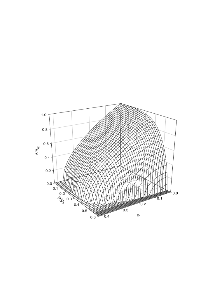
FIG. 1.: The pairing gap $\Delta(p_{F})$ in the ${}^{3}S_{1}$-${}^{3}D_{1}$ partial wave channel as a function of the isospin asymmetry $\alpha\equiv(\rho_{n}-\rho_{p})/\rho$ and total momentum $P$ in units of the Fermi momentum. The pairing gap is normalized to its value in the symmetric and zero-total-momentum case $\Delta_{00}=14.38$ MeV at fixed total density $\rho=0.16$ fm^-3 and temperature $\beta^{-1}=3$ MeV.

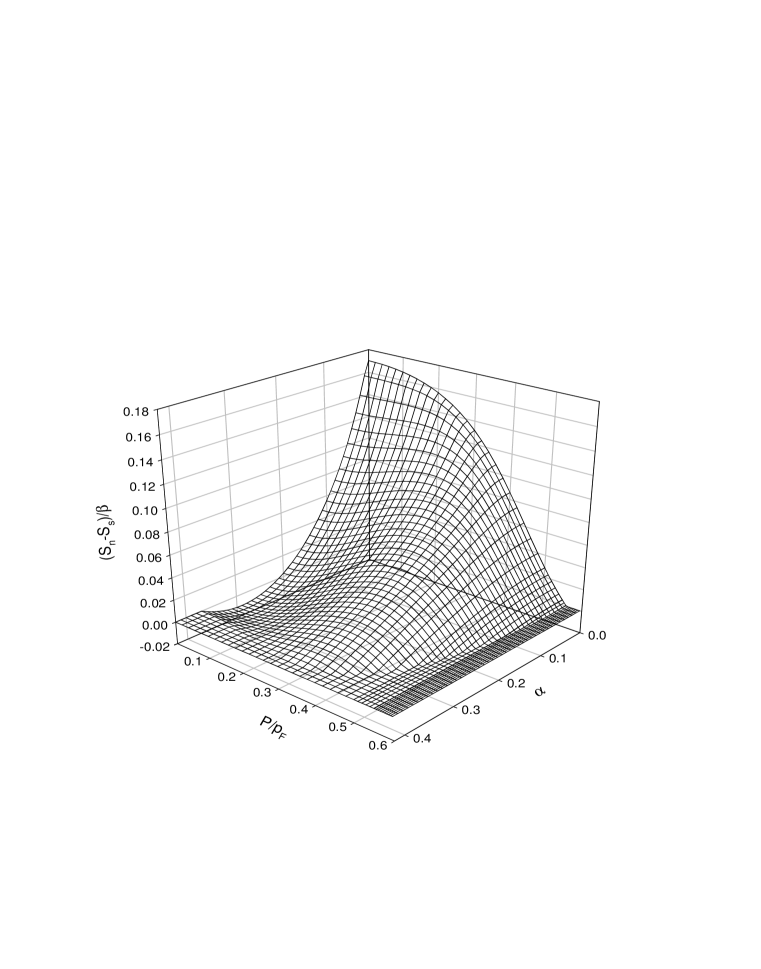
FIG. 2.: The latent heat of transition as a function of isospin asymmetry $\alpha$ and total momentum $P$. The remaining parameters are the same as in Fig. 1.

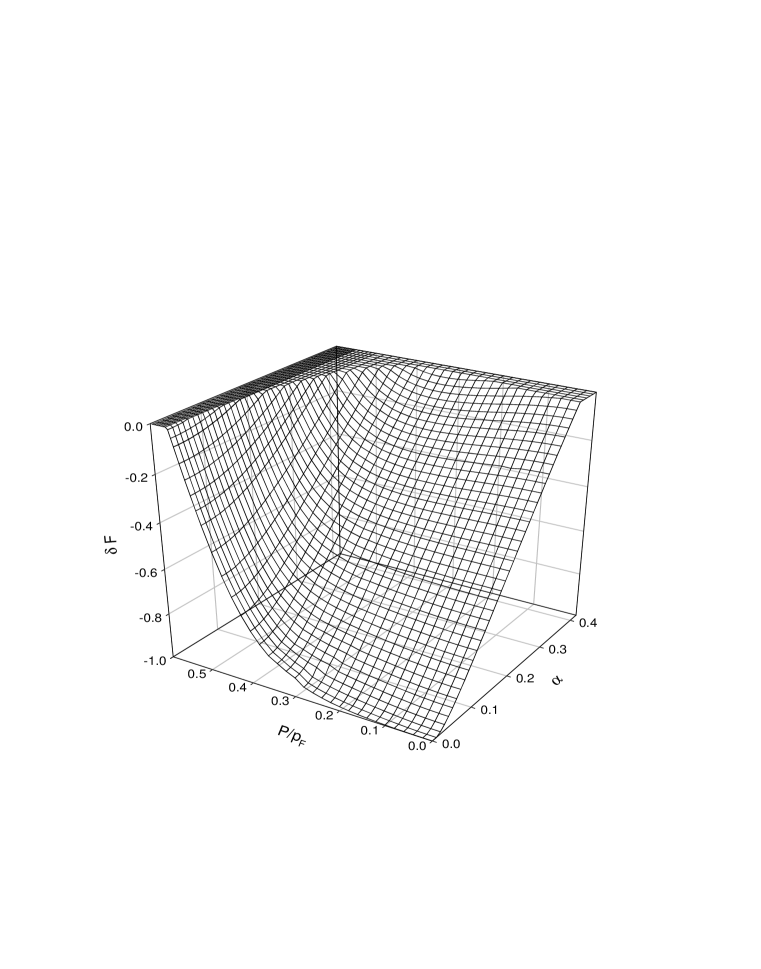
FIG. 3.: The difference of the free energies of the normal and superconducting state $(\delta F)_{\rho\beta}$, normalized to its value in the symmetric and zero-total-momentum state $(\delta F_{00})_{\rho\beta}=-7.35$ MeV. The remaining parameters are the same as in Fig. 1.

REFERENCES

- [1] A. A. Abrikosov and L. P. Gor’kov, Zh. Eksp. Teor. Fiz. 39, 1781 (1961) [Sov. Phys. JETP 12, 1243 (1961)].
- [2] A. M. Clogston, Phys. Rev. Lett. 9, 266 (1962).
- [3] B. S. Chandrasekhar, Appl. Phys. Lett. 1, 7 (1962).
- [4] L. P. Gor’kov and A. I. Rusinov, Zh. Eksp. Teor. Fiz. 46, 1363 (1964) [Sov. Phys. JETP 19, 922 (1964)].
- [5] T. Alm, B. L. Friman, G. Röpke, and H. Schulz, Nucl. Phys. A551, 45 (1993).
- [6] M. Baldo, U. Lombardo, and P. Schuck, Phys. Rev. C 52, 975 (1995).
- [7] T. Alm, G. Röpke, A. Sedrakian, and F. Weber, Nucl. Phys. A604, 491 (1996).
- [8] A. Sedrakian, T. Alm, and U. Lombardo, Phys. Rev. C 55, R582 (1997).
- [9] A. Sedrakian and U. Lombardo, Phys. Rev. Lett. 84, 602 (2000).
- [10] G. Röpke, A. Schnell, P. Schuck, and U. Lombardo, Phys. Rev. C 61, 024306 (2000).
- [11] A. I. Akhiezer, A. A. Isayev, S. V. Peletminsky, and A. A. Yatsenko, Phys. Rev. C, in press, nucl-th/0004040.
- [12] M. Alford, J. Berges, and K. Rajagopal, Phys. Rev. Lett. 84, 598 (2000).
- [13] P. Bedaque, hep-ph/9910247.
- [14] A. I. Larkin and Yu. N. Ovchinnikov, Zh. Eksp. Teor. Fiz. 47, 1136 (1964) [Sov. Phys. JETP 20, 762 (1965)].
- [15] P. Fulde and R. A. Ferrell, Phys. Rev. 135, 550 (1964).
- [16] M. Alford, J. Bowers, and K. Rajagopal, hep-ph/0008208.
- [17] R. Rapp, E. V. Shuryak, and I. Zahed, hep-ph/0008207.
- [18] A. L. Goodman, Phys. Rev. C 60, 014311 (1999) and references therein.
- [19] G. Martínez-Pinedo, K. Langanke, and P. Vogel, Nucl. Phys. A651, 379 (1999).
- [20] G. E. Brown and H. A. Bethe, Astrophys. J. 423, 659 (1994).
- [21] N. K. Glendenning, Compact Stars (Springer, New York, 1996) and references therein.
- [22] J. Haidenbauer and W. Plessas, Phys. Rev. C 30, 1822 (1984).