Neutrino-Deuteron Scattering in Effective Field Theory at Next-to-Next-to Leading Order

Abstract

We study the four channels associated with neutrino-deuteron breakup reactions at next-to-next to leading order in effective field theory. We find that the total cross-section is indeed converging for neutrino energies up to 20 MeV, and thus our calculations can provide constraints on theoretical uncertainties for the Sudbury Neutrino Observatory. We stress the importance of a direct experimental measurement to high precision in at least one channel, in order to fix an axial two-body counterterm.

I Introduction

Our understanding of electroweak processes on the deuteron is reaching a critical juncture. The Sudbury Neutrino Observatory is taking data, and a thorough understanding of neutrino-deuteron scattering is an important part of the analysis in that experiment [1, 2]. Of further note, there is a proposal for a high-precision measurement of the reaction $\nu_{e}d\rightarrow e^{-}pp$ in the ORLAND experiment [3].

Theorists have made a tremendous effort to understand $\nu(\overline{\nu})$-$d$ scattering in a potential model framework [4, 5, 6, 7, 8, 9, 10], with the most recent independent efforts agreeing within a few percent at low-energy  [11, 12]. Given the ongoing experimental interest in these processes, efforts began to study $\nu(\overline{\nu})$-$d$ scattering in the language of effective field theory (EFT) [13] for neutrino energies below 20 MeV. The EFT work employed the power-counting scheme of Kaplan, Savage, and Wise[14] and included pions. In working to next-to-leading order (NLO), it was found in ref. [13] that theoretical uncertainties in the reactions $\nu d\rightarrow\nu np$, $\overline{\nu}d\rightarrow\overline{\nu}np$, and $\overline{\nu}_{e}d\rightarrow e^{+}nn$ were dominated by an unknown axial two-body counterterm $L_{1,A}$. It was possible to find different values of $L_{1,A}$ which provided excellent fits to the potential model calculations of refs. [10, 11]. Further, we found that the ratio of charged-current to neutral current (CC/NC) cross-sections was insensitive to this counterterm. This confirmed the insensitivity to short-distance physics first discussed by ref. [11]. However, it is not clear whether a power-counting scheme exists which would allow us to extend the theory with pions to higher-order [15, 16, 17, 18], as would be required to constrain our theoretical uncertainties.

In this work, we employ the theory without pions [19] (also see earlier works [14, 20, 21, 22, 23, 24, 25, 26]) which has proven so successful in providing for high-precision calculations for other processes like $np\rightarrow d\gamma$ [27, 28]. This allows us to consider next-to-next-to leading order (NNLO) corrections, and to incorporate Coulomb effects cleanly, following the prescription of Kong and Ravndal [29] with some generalization. As a result, we present a complete set of calculations for all four reaction channels including the most-important $pp$ channel. No new parameters are introduced at this order, so it becomes a stringent test of the convergence of the calculation and thus on the theoretical uncertainties. Further, new potential model calculations exist  [12] and a further comparison with those is worthwhile, given that these new calculations yield different results at threshold to those in ref.  [10]. We continue to emphasize the importance of fixing the axial counterterm through a direct experimental measurement. This has implications not only for neutrino-deuteron scattering, but also for $pp\rightarrow de^{+}\nu_{e}$, $NN\rightarrow NN\overline{\nu}\nu$, and parity violating $\vec{e}$-$d$ scattering.

II The Lagrangian

We will briefly review nuclear effective field theory without pions [19]. The dynamical degrees of freedom are nucleons and non-hadronic external currents. Massive hadronic excitations such as pions and the delta are treated as non-dynamical, point interactions whose effects are encoded in the local operators in the lagrangian. The nucleons are non-relativistic but with relativistic corrections built in systematically. Nuclear interaction processes are calculated perturbatively with the small expansion parameter

$$Q\equiv\frac{(1/a,\gamma,p,\left|{\bf q}\right|)}{\Lambda}$$ (1)

which is the ratio of the light to heavy scales. The light scales include the inverse S-wave nucleon-nucleon scattering length $1/a(\lesssim 12$ MeV$)$ in the ${}^{1}S_{0}$ channel, the deuteron binding momentum $\gamma(=45.69$ MeV) in the ${}^{3}S_{1}$ channel, the magnitude of the nucleon external momentum $p$ in the two nucleon center-of-mass frame, and the momentum transfer to the two nucleon system $\left|{\bf q}\right|$. The heavy scale $\Lambda$ is set by the pion mass $m_{\pi}$. How each term in the lagrangian scales as powers of $Q$ can be found in ref. [19]. It is the nontrivial renormalization of the strong interaction operators makes the scaling different from a naive derivative expansion [14].

A The Effective Lagrangian

The lagrangian of an effective field theory for nucleons can be described via

$${\cal L}={\cal L}_{1}+{\cal L}_{2}+\cdots\quad,$$ (2)

where ${\cal L}_{n}$ contains operators involving $n$ nucleons. Neglecting for the moment the weak-interaction couplings, we have

$${\cal L}_{1}=N^{\dagger}\bigg{(}iD_{0}+{\frac{{\bf D}^{2}}{2M_{N}}}-\frac{D_{0}^{2}}{2M_{N}}\bigg{)}N\quad,$$ (3)

where $N$ is the nucleon field, $M_{N}$ is the nucleon mass, $D_{0}$ and ${\bf D}$ are covariant derivatives and the $D_{0}^{2}$ term is the leading relativistic correction.

The two-nucleon lagrangian needed for a calculation to NNLO is

$${\cal L}_{2} = -C_{0}^{(\,^{3}S_{1})}(N^{T}P_{i}N)^{\dagger}(N^{T}P_{i}N)$$ (9)

$$+{\frac{C_{2}^{(\,^{3}S_{1})}}{8}}\left[(N^{T}P_{i}N)^{\dagger}(N^{T}(\overleftarrow{{\bf D}}^{2}P_{i}-2\overleftarrow{{\bf D}}\cdot P_{i}\overrightarrow{{\bf D}}+P_{i}\overrightarrow{{\bf D}}^{2})N)+h.c.\right]$$

$$-{\frac{C_{4}^{(\,^{3}S_{1})}}{16}}\bigg{(}N^{T}\bigg{[}P_{i}\overrightarrow{{\bf D}}^{2}+\overleftarrow{{\bf D}}^{2}P_{i}-2\overleftarrow{{\bf D}}P_{i}\overrightarrow{{\bf D}}\bigg{]}N\bigg{)}^{\dagger}\bigg{(}N^{T}\bigg{[}P_{i}\overrightarrow{{\bf D}}^{2}+\overleftarrow{{\bf D}}^{2}P_{i}-2\overleftarrow{{\bf D}}P_{i}\overrightarrow{{\bf D}}\bigg{]}N\bigg{)}$$

$$-C_{0}^{(\,^{1}S_{0},i)}(N^{T}\overline{P}_{i}N)^{\dagger}(N^{T}\overline{P}_{i}N)$$

$$+{\frac{C_{2}^{(\,^{1}S_{0},i)}}{8}}\left[(N^{T}\overline{P_{i}}N)^{\dagger}(N^{T}(\overleftarrow{{\bf D}}^{2}\overline{P}_{i}-2\overleftarrow{{\bf D}}\cdot\overline{P}_{i}\overrightarrow{{\bf D}}+\overline{P}_{i}\overrightarrow{{\bf D}}^{2})N)+h.c.\right]$$

$$-{\frac{C_{4}^{(\,^{1}S_{0},i)}}{16}}\bigg{(}N^{T}\bigg{[}\overline{P}_{i}\overrightarrow{{\bf D}}^{2}+\overleftarrow{{\bf D}}^{2}\overline{P}_{i}-2\overleftarrow{{\bf D}}\overline{P}_{i}\overrightarrow{{\bf D}}\bigg{]}N\bigg{)}^{\dagger}\bigg{(}N^{T}\bigg{[}\overline{P}_{i}\overrightarrow{{\bf D}}^{2}+\overleftarrow{{\bf D}}^{2}\overline{P}_{i}-2\overleftarrow{{\bf D}}\overline{P}_{i}\overrightarrow{{\bf D}}\bigg{]}N\bigg{)}\quad,$$

where $P_{i}$ and $\overline{P}_{i}$ are spin-isospin projectors for the ${}^{3}S_{1}$ channel and the ${}^{1}S_{0}$ channel respectively,

$$P_{i} \equiv \frac{1}{\sqrt{8}}\sigma_{2}\sigma_{i}\tau_{2}\quad,\quad\text{Tr}P_{i}^{\dagger}P_{j}=\frac{1}{2}\delta_{ij}\quad,$$ (10)

$$\overline{P}_{i} \equiv \frac{1}{\sqrt{8}}\sigma_{2}\tau_{2}\tau_{i}\quad,\quad\text{Tr}\overline{P}_{i}^{\dagger}\overline{P}_{j}=\frac{1}{2}\delta_{ij}\quad,$$ (11)

with the $\tau$ matrices act on isospin indices and $\sigma$ matrices on the spin indices. We incorporate isospin symmetry breaking in the $C_{2n}^{(\,^{1}S_{0},i)}(n=0,1,...)$ operators, so that $C_{2n}^{(\,^{1}S_{0},pp)}$, $C_{2n}^{(\,^{1}S_{0},np)}$ and $C_{2n}^{(\,^{1}S_{0},nn)}$ are different. In both the ${}^{3}S_{1}$ and ${}^{1}S_{0}$ channels, the strong coupling constants $C_{2n}$ have renormalization scale ($\mu$) dependence. These parameters can be fit to the effective range expansion, as detailed in ref.  [19] and as reviewed in Appendix A.

Relativistic corrections start to contribute to physical quantities at NNLO and have generic sizes of ${\cal O}(p^{2}/m_{N}^{2})$ of the leading-order (LO) contribution (see [19] for examples). They are suppressed by an additional factor of $\Lambda^{2}/m_{N}^{2}$ to other NNLO contributions, and thus we can neglect them as small (this is verified numerically).

B Weak Interactions

The effective lagrangians for charged (CC) and neutral current (NC) weak interactions are given by

$${\cal L}^{CC}\ =-{\displaystyle{\frac{G_{F}}{\sqrt{2}}}}l_{+}^{\mu}J_{\mu}^{-}+h.c.\quad,$$ (12)

$${\cal L}^{NC}\ =-{\displaystyle{\frac{G_{F}}{\sqrt{2}}}}l_{Z}^{\mu}J_{\mu}^{Z}\quad,$$ (13)

where the $l_{\mu}$ is the leptonic current and $J_{\mu}$ is the hadronic current. We have used $G_{F}=1.166\times 10^{-5}$ GeV^-2. For $\nu$-$d$ and $\overline{\nu}$-$d$ scattering,

$$l_{+}^{\mu}=\overline{\nu}\gamma^{\mu}(1-\gamma_{5})e\quad,\quad l_{Z}^{\mu}=\overline{\nu}\gamma^{\mu}(1-\gamma_{5})\nu\quad.$$ (14)

The hadronic currents can be decomposed into vector and axial-vector contributions

$$J_{\mu}^{-} = V_{\mu}^{-}-A_{\mu}^{-}=(V_{\mu}^{1}-A_{\mu}^{1})-i(V_{\mu}^{2}-A_{\mu}^{2})\quad,$$ (15)

$$J_{\mu}^{Z} = -2\sin^{2}\theta_{W}V_{\mu}^{S}+(1-2\sin^{2}\theta_{W})V_{\mu}^{3}-A_{\mu}^{S}-A_{\mu}^{3}\quad,$$ (16)

where the superscripts represent isovector components (with $S$ representing isoscalar terms) and, later, the currents will be labeled by the number of nucleons involved.

In a NNLO calculation, the electron mass $m_{e}$ contributions to the matrix elements are counted as higher order (suppressed by a factor of $m_{e}^{2}/\gamma^{2}$), such that $q_{\mu}l^{\mu}=0$ up to NNLO. Similarly, if the neutrino mass $m_{\nu}\neq 0$ but $m_{\nu}^{2}/\gamma^{2}\ll 1$, then the massless neutrino treatment we have here is still applicable. The non-relativistic one-body currents are given by

$$V_{0}^{(1)} = \frac{1}{2}N^{\dagger}(1+\tau_{a})N\quad,$$ (17)

$$A_{0}^{(1)} = -{\frac{i}{2}}N^{\dagger}(\Delta s-g_{A}\tau_{a}){\frac{{\bf\sigma}\cdot(\overleftarrow{{\bf\nabla}}-\overrightarrow{{\bf\nabla}})}{2M_{N}}}N\quad,$$ (18)

$$V_{k}^{(1)} = {\frac{i}{2}}N^{\dagger}(1+\tau_{a}){\frac{(\overleftarrow{\nabla}_{k}-\overrightarrow{\nabla}_{k})}{2M_{N}}}N-N^{\dagger}\bigg{(}\kappa^{(0)}+\frac{\mu_{s}}{4\sin^{2}\theta_{W}}+\kappa^{(1)}\tau_{a}\bigg{)}\epsilon_{kij}{\frac{\sigma_{i}(\overleftarrow{\nabla}_{j}+\overrightarrow{\nabla}_{j})}{2M_{N}}}N\quad,$$ (19)

$$A_{k}^{(1)} = -{\frac{1}{2}}N^{\dagger}(\Delta s-g_{A}\tau_{a})\sigma_{k}N\quad,$$ (20)

where $g_{A}=1.26$. Here we have neglected the nucleon vector and axial vector charge radius contributions. They only contribute at NNLO with about the same size as the relativistic contributions due to the small momentum transfers being considered here.

We use the notation $\Delta s$ for the strange quark contribution to the proton spin

$$2S_{\mu}\Delta s\equiv\left\langle p\left|\overline{s}\gamma_{\mu}\gamma_{5}s\right|p\right\rangle\quad$$ (21)

with the value [30]

$$\Delta s=-0.17\pm 0.17\>,$$ (22)

where $S_{\mu}$ is the covariant spin vector. $\kappa^{(0)}=\frac{1}{2}(\kappa_{p}+\kappa_{n})$ and $\kappa^{(1)}=\frac{1}{2}(\kappa_{p}-\kappa_{n})$ are the conventional isoscalar and isovector nucleon magnetic moments in nuclear magnetons, with

$$\kappa_{p}=2.79285\quad,\quad\kappa_{n}=-1.91304\quad.$$ (23)

$\mu_{s}$ is the strange magnetic moment of the proton [31]

$$\left\langle p\left|\overline{s}\gamma_{\mu}s\right|p\right\rangle=\overline{u}_{p}\bigg{(}F_{1}^{s}(q^{2})\gamma_{\mu}+F_{2}^{s}(q^{2})\frac{i\sigma_{\mu\nu}q^{\nu}}{2M_{N}}\bigg{)}u_{p}\quad,$$ (24)

$$G_{M}^{s}(q^{2})\equiv F_{1}^{s}(q^{2})+F_{2}^{s}(q^{2})\quad,$$ (25)

$$F_{1}^{s}(0)=0\quad,\quad\mu_{s}\equiv G_{M}^{s}(0)\quad.$$ (26)

In ref. [32], the SAMPLE experiment found

$$G_{M}^{s}(-0.1{\rm GeV}^{2})=0.23\pm 0.37\pm 0.15\pm 0.19\text{ }{\rm n.m.}\>,\quad$$ (27)

extracted from the proton target experiment. However, the newest deuteron target measurement suggests that the radiative corrections to the axial form factor were underestimated. Thus the central value of $G_{M}^{s}(-0.1{\rm GeV}^{2})$ could be 40% smaller [33]. Theoretical predictions for $\mu_{s}$ range from -0.8 n.m. to 0.8 n.m..

Finally, there are two-body currents relevant to this process. As mentioned in ref. [13], there are axial contributions

$$A_{k}^{(2)}=L_{1,A}\left(N^{T}P_{k}N\right)^{\dagger}\left(N^{T}\overline{P}_{a}N\right)-2i\varepsilon_{ijk}L_{2,A}(N^{T}P_{i}N)^{\dagger}(N^{T}P_{j}N)+h.c.\quad,$$ (28)

and analogous vector contributions to the deuteron magnetic properties, as described in ref. [19, 14]

$$V_{k}^{(2)} = e\varepsilon_{kij}L_{1}\left(N^{T}P_{i}N\right)^{\dagger}(\overleftarrow{\nabla}_{j}+\overrightarrow{\nabla}_{j})\left(N^{T}\overline{P}_{a}N\right)$$ (30)

$$-2ieL_{2}(N^{T}P_{i}N)^{\dagger}(\overleftarrow{\nabla}_{i}+\overrightarrow{\nabla}_{i})(N^{T}P_{k}N)+h.c.\quad.$$

The parameters $L_{1}$ and $L_{2}$ can be fit from $np\rightarrow d\gamma$ and the deuteron magnetic moment, respectively, and are given by $L_{1}=7.24$ fm⁴ and $L_{2}=-0.149$ fm⁴ at $\mu=m_{\pi}$[19].

III $\nu(\bar{\nu})$-$D$ Neutral Current Inelastic Scattering

For the inelastic scattering process

$$\nu+d\rightarrow\nu+n+p,$$ (31)

the differential cross section can be written in terms of leptonic and hadronic tensors $l_{\mu\nu}$ and $W_{\mu\nu}$ as

$${\displaystyle{d^{2}\sigma\over d\omega^{{}^{\prime}}d\Omega}}={\displaystyle{G_{F}^{2}\left|{\bf k}^{\prime}\right|\over 32\pi^{2}\left|{\bf k}\right|}}S_{1}(\left|{\bf k}^{\prime}\right|)\ l^{\mu\nu}W_{\mu\nu}\quad,$$ (32)

where $\omega(\omega^{\prime})=k_{0}(k_{0}^{\prime})$ represent the initial(final) neutrino energies.

$$S_{1}(\left|{\bf k}^{\prime}\right|)=1$$ (33)

for NC processes. The leptonic tensor is given by

$$\ l^{\mu\nu}=8(k^{\mu}k^{\nu\prime}+k^{\nu}k^{\mu\prime}-k\cdot k^{\prime}g^{\mu\nu}+i\varepsilon^{\mu\nu\rho\sigma}k_{\rho}k_{\sigma}^{{}^{\prime}})\quad.$$ (34)

The hadronic tensor is the imaginary part of forward matrix element of the time order product of two weak current operators. It can be parameterized by six different structure functions

$$W_{\mu\nu} = {\displaystyle{1\over\pi}}\text{Im}\left[\displaystyle\int d^{4}xe^{iqx}T\left\langle d(P)\left|J_{\mu}^{Z^{\dagger}}(x)J_{\nu}^{Z}(0)\right|d(P)\right\rangle\right]$$ (35)

$$= -W_{1}g_{\mu\nu}+W_{2}{\displaystyle{P_{\mu}P_{\nu}\over M_{d}^{2}}}-iW_{3}\varepsilon_{\mu\nu\alpha\beta}{\displaystyle{P^{\alpha}q^{\beta}\over M_{d}^{2}}}$$ (37)

$$+W_{4}{\displaystyle{q_{\mu}q_{\nu}\over M_{d}^{2}}}+W_{5}{\displaystyle{(P_{\mu}q_{\nu}+q_{\mu}P_{\nu})\over M_{d}^{2}}}+iW_{6}{\displaystyle{(P_{\mu}q_{\nu}-q_{\mu}P_{\nu})\over M_{d}^{2}}}\quad,$$

where the momentum transfer $q_{\mu}=k_{\mu}-k_{\mu}^{\prime}$. We can easily see that $W_{4},W_{5}$ and $W_{6}$ don’t contribute to the differential cross section because $q_{u}l^{\mu\nu}=0$. In the lab frame (deuteron rest frame) the differential cross-section simplifies to

$${\displaystyle{d^{2}\sigma\over d\omega^{{}^{\prime}}d\Omega}}={\displaystyle{G_{F}^{2}\omega^{\prime}\left|{\bf k}^{\prime}\right|\over 2\pi^{2}}}S_{1}(\left|{\bf k}^{\prime}\right|)\left[2W_{1}\sin^{2}{\displaystyle{\theta\over 2}}+W_{2}\cos^{2}{\displaystyle{\theta\over 2}}-2{\displaystyle{(\omega+\omega^{\prime})\over M_{d}}}W_{3}\sin^{2}{\displaystyle{\theta\over 2}}\right]\quad,$$ (38)

where the $\theta$ is the angle between k and k${}^{{}^{\prime}}$ and we have used the relation

$$q^{2}=-4\omega\omega^{\prime}\sin^{2}{\displaystyle{\theta\over 2}}\quad.$$ (39)

For $\overline{\nu}d\ \rightarrow\overline{\nu}np$ scattering, the last terms on the right hand sides of eq.(34) and (38) change sign.

Phase space for this reaction is defined by

$$\text{Max}\left[-1,1-{\displaystyle{4M_{N}(\nu-B)-\nu^{2}\over 2\omega\omega^{\prime}}}\right]\leq\cos\theta\leq 1\quad,$$ (40)

and

$$0\leq\omega^{\prime}\leq\omega-2(M_{N}-\sqrt{M_{N}^{2}-\gamma^{2}})\quad,$$ (41)

where $\nu=\omega-\omega^{\prime}$, $M_{N}$ is the nucleon mass and $B(=2.2245$ MeV) is the deuteron binding energy.

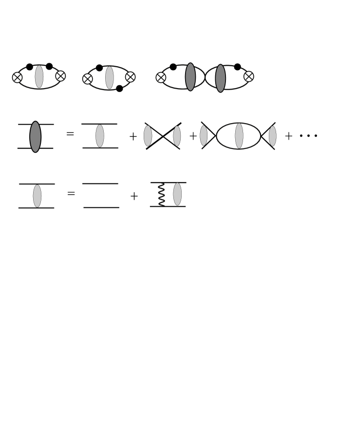
FIG. 1.: Diagrams that contribute to $W_{0}$ and $W_{1}$ at leading order. The crossed circles denote operators that create or annihilate two nucleons with the quantum numbers of the deuteron. The dark gray blobs arise from scattering corrections involving insertions of $C_{0}$ operators of the appropriate channel, and from the Coulomb Green’s function (the light gray blob). The wavy line represents the Coulomb interaction, present only in the $pp$ final state. Solid lines represent nucleons, and the solid circles represent insertions of electroweak current operators.

In the deuteron rest frame,

$$W_{0} \equiv W_{00}=W_{2}-W_{1}\quad,\$$ (42)

$$W_{0i} = 0\quad,\$$ (43)

$$W_{ij} \equiv \delta_{ij}W_{1}-iW_{3}\varepsilon_{0ijk}{\displaystyle{q^{k}\over M_{d}}}\quad.$$ (44)

The structure function can be $Q$ expanded as

$$W_{\mu\nu}=W_{\mu\nu}^{LO}+W_{\mu\nu}^{NLO}+W_{\mu\nu}^{NNLO}+\cdots\qquad.$$ (45)

Now we give the expressions for the structure functions order by order in the perturbative expansion.

A Leading Order (LO)

The LO diagrams in fig. 1 give

$$W_{0}^{LO} = \left[2(C_{V}^{(0)^{2}}+C_{V}^{(1)^{2}})F_{1}+(C_{V}^{(0)^{2}}-C_{V}^{(1)^{2}})F_{2}+4C_{V}^{(0)^{2}}F_{3}^{LO}\right]\quad,$$ (46)

$$W_{1}^{LO} = \left[2(C_{A}^{(0)^{2}}+C_{A}^{(1)^{2}})F_{1}+{\displaystyle{1\over 3}}(C_{A}^{(0)^{2}}-C_{A}^{(1)^{2}})F_{2}+\frac{8}{3}C_{A}^{(0)^{2}}F_{3}^{LO}+\frac{4}{3}C_{A}^{(1)^{2}}F_{4}^{LO}\right]\ \quad,$$ (47)

$$W_{3}^{LO} = 0\qquad.$$ (48)

The vector and axial-vector coupling coefficients are given by

$$\begin{array}[]{ll}C_{V}^{(0)}=-\sin^{2}\vartheta_{W}&,\quad C_{V}^{(1)}={\displaystyle{1\over 2}}(1-2\sin^{2}\vartheta_{W})\quad,\\ C_{A}^{(0)}=-{\displaystyle{1\over 2}}\Delta s&,\quad C_{A}^{(1)}={\displaystyle{1\over 2}}g_{A}\quad.\end{array}$$ (49)

The structure and interaction effects are contained in

$$F_{1} = {\displaystyle{2M_{N}\gamma\ p\over\pi\left(p^{2}+\gamma^{2}\right)^{2}}}S_{2}\left(p,|{\bf q}|\right)\quad,$$ (50)

$$F_{2} = {\displaystyle{4M_{N}\gamma\ p\over\pi\left(p^{2}+\gamma^{2}\right)^{2}}}S_{3}\left(p,|{\bf q}|\right)\quad,$$ (51)

$$F_{3}^{LO} = {\displaystyle{1\ \over\pi}}\text{Im}\left[B_{0}(p,\left|{\bf q}\right|{\bf)}^{2}A_{-1}^{(^{3}S_{1})}(p)\right]\quad,$$ (52)

$$F_{4}^{LO} = F_{3}^{LO}(^{3}S_{1}\rightarrow\ ^{1}S_{0})\ \quad.$$ (53)

The magnitude of the relative momentum between the final-state nucleons is $2p$, with

$$p=\sqrt{M_{N}\nu-\gamma^{2}-\frac{{\bf q}^{2}}{4}+i\epsilon}\quad,$$ (54)

where $\epsilon=0^{+}$. For the NC process,

$$S_{2}\left(p,|{\bf q}|\right) = 1+\frac{{\bf q}^{2}\left(p^{2}-\gamma^{2}\right)}{2\left(p^{2}+\gamma^{2}\right)^{2}}\quad,\quad$$ (55)

$$S_{3}\left(p,|{\bf q}|\right) = 1-\frac{{\bf q}^{2}\left(p^{2}+3\gamma^{2}\right)}{6\left(p^{2}+\gamma^{2}\right)^{2}}\quad,$$ (56)

$$B_{0}(p,\left|{\bf q}\right|{\bf)} = {\bf-}\sqrt{\frac{\gamma}{2\pi}}\frac{M_{N}}{\gamma-ip}\left(1-\frac{{\bf q}^{2}}{12\left(\gamma-ip\right)^{2}}\right)\quad.$$ (57)

Note that we have further expanded the ${\bf q}^{2}$ dependence in powers of ${\bf q}^{2}/\left(p^{2}+\gamma^{2}\right)$ in order to later obtain analytic results for the Coulomb contribution in the $pp$ channel. The error introduced is numerically small ($\ll 1\%$ in total cross section) even though the neglected terms are formally LO.

The NN scattering amplitude has an expansion

$$A=A_{-1}+A_{0}+A_{1}+\cdots\qquad,$$ (58)

where the subscripts denote the powers in the small expansion parameter $Q$.

$$A_{-1}^{(^{3}S_{1})}(p) = {\displaystyle{-4\pi\over M_{N}}}{\displaystyle{1\over\gamma+ip}}\qquad,$$ (59)

$$A_{0}^{(^{3}S_{1})}(p) = {\displaystyle{-2\pi\over M_{N}}}{\displaystyle{\rho_{d\ }\left(p^{2}+\gamma^{2}\right)\over\left(\gamma+ip\right)^{2}}}\qquad,$$ (60)

$$A_{1}^{(^{3}S_{1})}(p) = {\displaystyle{-\pi\over M_{N}}}{\displaystyle{\rho_{d\ }^{2}\left(p^{2}+\gamma^{2}\right)^{2}\over\left(\gamma+ip\right)^{3}}}\qquad,$$ (61)

where $\rho_{d}=1.764$ fm. And

$$A_{-1}^{(^{1}S_{0})}(p) = {\displaystyle{-4\pi\over M_{N}}}{\displaystyle{1\over{\displaystyle{1\over a^{(^{1}S_{0})}}}+ip}}\qquad,$$ (62)

$$A_{0}^{(^{1}S_{0})}(p) = {\displaystyle{-2\pi\over M_{N}}}{\displaystyle{r_{0}^{(^{1}S_{0})}p^{2}\over\left({\displaystyle{1\over a^{(^{1}S_{0})}}}+ip\right)^{2}}}\qquad,$$ (63)

$$A_{1}^{(^{1}S_{0})}(p) = {\displaystyle{-\pi\over M_{N}}}{\displaystyle{r_{0}^{(^{1}S_{0})^{2}}p^{4}\over\left({\displaystyle{1\over a^{(^{1}S_{0})}}}+ip\right)^{3}}}\qquad,$$ (64)

where the scattering length $a^{(^{1}S_{0},np)}=-23.7$ fm is known to high accuracy while the effective range $r_{0}^{(^{1}S_{0},np)}=2.73$ fm has a 2% uncertainty [34]. This uncertainty is insignificant in this calculation.

B Next-to-Leading Order (NLO)

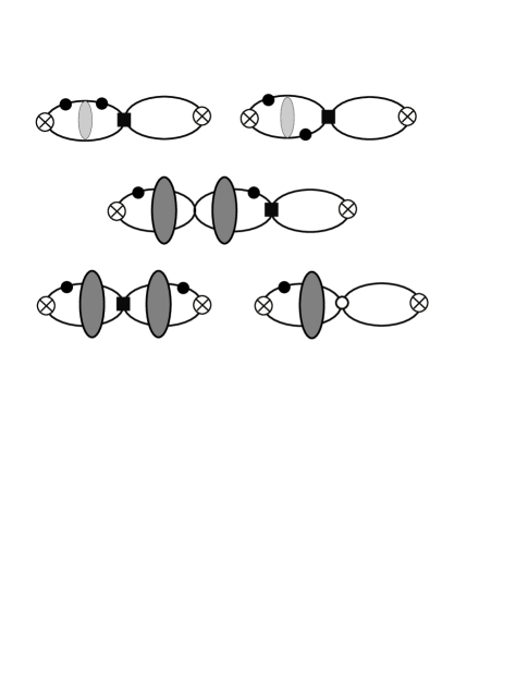
FIG. 2.: Diagrams at NLO that contribute to $W_{0}$ and $W_{1}$. The black square represents an insertion of the $C_{2}$ operator in the ${}^{1}S_{0}$ channel, and $C_{2,-2},\ C_{0,0}$ in the ${}^{3}S_{1}$ channel. The white circle represents an insertion of the two-body currents $L_{1,A}$ and $L_{2,A}$. Other features are as described in fig. 1.

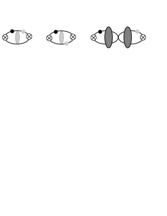
FIG. 3.: Diagrams at NLO that contribute to $W_{3}$. The light grey circle represents an insertion of the nucleon magnetic moment operator. Other features are as described in fig. 1.

At NLO, $W_{0}$ and $W_{1}$ receive contributions from fig. 2 while $W_{3}$ receives contributions from fig. 3.

$$W_{0}^{NLO} = \gamma\rho_{d}W_{0}^{LO}+4C_{V}^{(0)^{2}}F_{3}^{NLO}+G_{1}^{NLO}\quad,$$ (65)

$$W_{1}^{NLO} = \gamma\rho_{d}W_{1}^{LO}+\frac{8}{3}C_{A}^{(0)^{2}}F_{3}^{NLO}+\frac{4}{3}C_{A}^{(1)^{2}}F_{4}^{NLO}\ +G_{2}^{NLO}\quad,$$ (66)

$$W_{3}^{NLO} = -2\left[2(C_{A}^{(0)}C_{M}^{(0)}+C_{A}^{(1)}C_{M}^{(1)})F_{1}+{\displaystyle{1\over 3}}(C_{A}^{(0)}C_{M}^{(0)}-C_{A}^{(1)}C_{M}^{(1)})F_{2}+\frac{8}{3}C_{A}^{(0)}C_{M}^{(0)}F_{3}^{LO}\right.$$ (68)

$$\left.+\frac{4}{3}C_{A}^{(1)}C_{M}^{(1)}F_{4}^{LO}\right]\ \quad,$$

where

$$F_{3}^{NLO} = F_{3}^{LO}(A_{-1}^{(^{3}S_{1})}\rightarrow A_{0}^{(^{3}S_{1})})\qquad,$$ (69)

$$F_{4}^{NLO} = F_{4}^{LO}(A_{-1}^{(^{1}S_{0})}\rightarrow A_{0}^{(^{1}S_{0})})\qquad,$$ (70)

and

$$G_{1}^{NLO} = C_{V}^{(0)^{2}}{\displaystyle{2M_{N}\rho_{d}\over\pi}}\mathop{\rm Im}\left[\sqrt{\frac{2\gamma}{\pi}}B_{0}(p,\left|{\bf q}\right|{\bf)}\ A_{-1}^{(^{3}S_{1})}(p)\right]\quad,$$ (71)

$$G_{2}^{NLO} = -{\displaystyle{M_{N}\over 3\pi^{2}}}\mathop{\rm Im}\left[\sqrt{\frac{\gamma}{2\pi}}B_{0}(p,\left|{\bf q}\right|{\bf)}\left(C_{A}^{(1)}\widetilde{L}_{1,A}A_{-1}^{(^{1}S_{0})}(p)+4C_{A}^{(0)}\widetilde{L}_{2,A}A_{-1}^{(^{3}S_{1})}(p)\right)\right]\qquad.$$ (72)

Note that $G_{1}^{LO}=G_{2}^{LO}=0$. The $\widetilde{L}_{A}$’s are renormalization scale $\mu$-independent quantities defined as

$$\widetilde{L}_{1,A} = -\frac{4\pi\left(\mu-\gamma\right)}{M_{N}C_{0}^{(^{1}S_{0})}}\left[L_{1,A}-2\pi C_{A}^{(1)}\left(\frac{M_{N}}{2\pi}C_{2}^{(^{1}S_{0})}+\frac{\rho_{d}}{\left(\mu-\gamma\right)^{2}}\right)\right]\quad,$$ (73)

$$\widetilde{L}_{2,A} = \left(\mu-\gamma\right)^{2}L_{2,A}-2\pi C_{A}^{(0)}\rho_{d}\quad.$$ (74)

The expressions for $C_{0}^{(^{1}S_{0})}$ and $C_{2}^{(^{1}S_{0})}$ can be found in Appendix A. Through $W_{3}$, we become sensitive to weak magnetism at NLO, with coupling coefficients given by

$$\begin{array}[]{ll}C_{M}^{(0)}=-2\sin^{2}\vartheta_{W}\kappa^{(0)}-\frac{1}{2}\mu_{S}&,\quad C_{M}^{(1)}=(1-2\sin^{2}\vartheta_{W})\kappa^{(1)}\quad.\end{array}$$ (75)

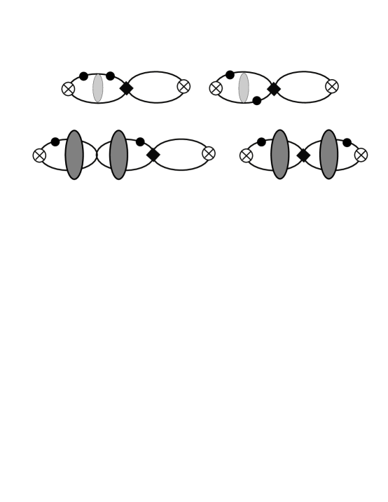
FIG. 4.: Diagrams at NNLO that contribute to $W_{0}$ and $W_{1}$. The black diamond represents an insertion of the $C_{4}$ operator in the ${}^{1}S_{0}$ channel, and $C_{4,-3},\ C_{2,-1},\ C_{0,1}$ in the ${}^{3}S_{1}$ channel. Other features are as described in fig. 1.

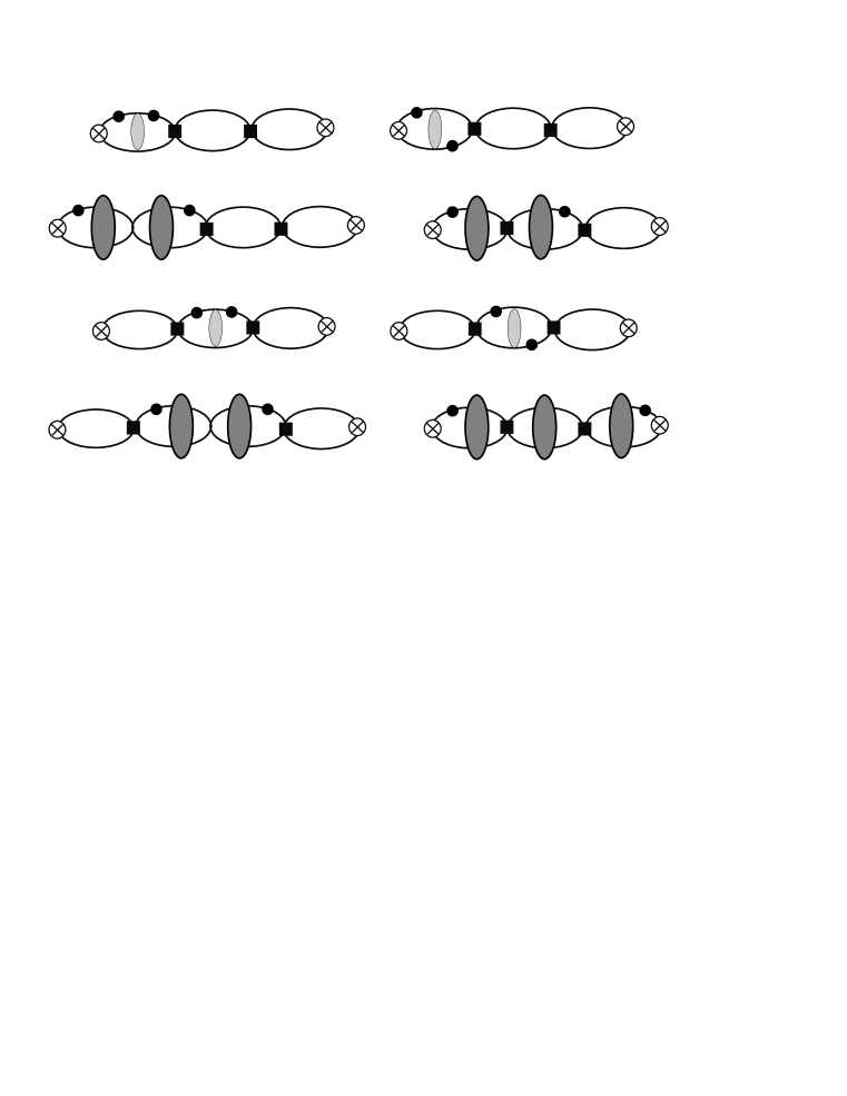
FIG. 5.: Diagrams at NNLO that contribute to $W_{0}$ and $W_{1}$ through two insertions (black squares) of the $C_{2}$ operator in the ${}^{1}S_{0}$ channel, and $C_{2,-2},\ C_{1,0}$ in the ${}^{3}S_{1}$ channel. Other features are as described in fig. 1.

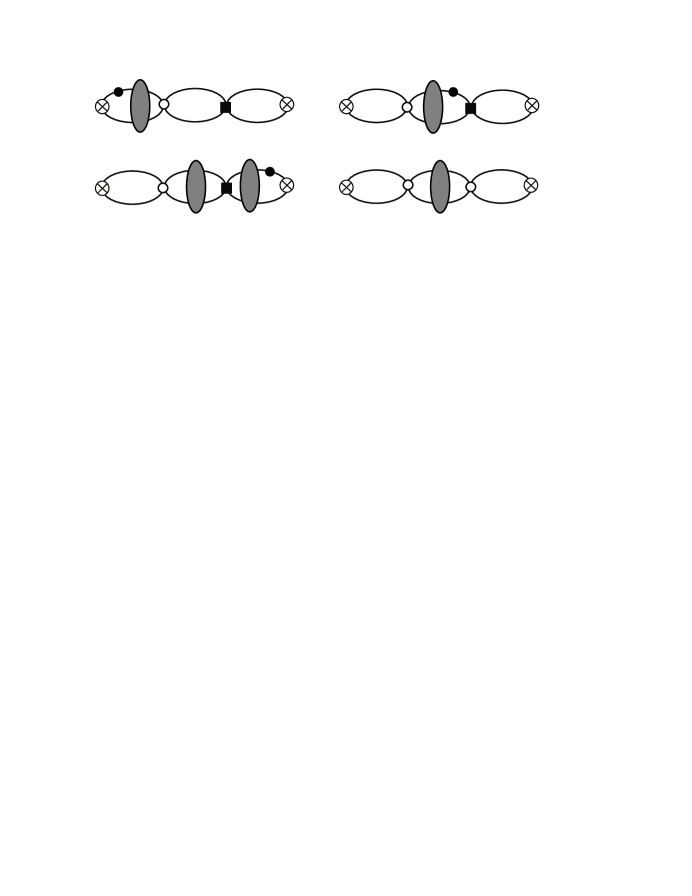
FIG. 6.: Diagrams at NNLO that contribute to $W_{0}$ and $W_{1}$ through mixed insertions of the $L_{1,A}$ and $L_{2,A}$ operators (white circle) and $C_{2}$ operators (black square). Other features are as described in fig. 1.

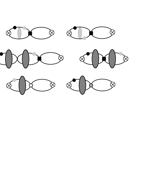
FIG. 7.: Diagrams at NNLO that contribute to $W_{3}$. The filled circle represents an insertion of the two-body current $L_{1}$ or $L_{2}$. Other features are as described in figs. 1 and 2.

C Next-to-Next-to-Leading Order (NNLO)

Finally, at NNLO, $W_{0}$ and $W_{1}$ receive contributions from figs. 4-6 while $W_{3}$ receives contributions from fig. 7.

$$W_{0}^{NNLO} = \gamma\rho_{d}W_{0}^{NLO}+4C_{V}^{(0)^{2}}F_{3}^{NNLO}+G_{1}^{NNLO}\quad,$$ (76)

$$W_{1}^{NNLO} = \gamma\rho_{d}W_{1}^{NLO}+\frac{8}{3}C_{A}^{(0)^{2}}F_{3}^{NNLO}+\frac{4}{3}C_{A}^{(1)^{2}}F_{4}^{NNLO}\ +G_{2}^{NNLO}\quad,$$ (77)

$$W_{3}^{NNLO} = \gamma\rho_{d}W_{3}^{NLO}-2\left(\frac{8}{3}C_{A}^{(0)}C_{M}^{(0)}F_{3}^{NLO}+\frac{4}{3}C_{A}^{(1)}C_{M}^{(1)}F_{4}^{NLO}+G_{3}^{NLO}\right)\qquad,$$ (78)

where

$$F_{3}^{NNLO} = F_{3}^{LO}(A_{-1}^{(^{3}S_{1})}\rightarrow A_{1}^{(^{3}S_{1})})\qquad,$$ (79)

$$F_{4}^{NNLO} = F_{4}^{LO}(A_{-1}^{(^{1}S_{0})}\rightarrow A_{1}^{(^{1}S_{0})})\qquad.$$ (80)

$$G_{1}^{NNLO} = G_{1}^{NLO}(A_{-1}^{(^{3}S_{1})}\rightarrow A_{0}^{(^{3}S_{1})})+C_{V}^{(0)^{2}}{\displaystyle{\gamma M_{N}^{2}\rho_{d}^{2}\over 2\pi^{2}}}\mathop{\rm Im}\left[A_{-1}^{(^{3}S_{1})}(p)\right]\quad,$$ (81)

$$G_{2}^{NNLO} = G_{2}^{NLO}(A_{-1}^{(^{3}S_{1})}\rightarrow A_{0}^{(^{3}S_{1})},A_{-1}^{(^{1}S_{0})}\rightarrow A_{0}^{(^{1}S_{0})})$$ (83)

$$+{\displaystyle{M_{N}^{2}\gamma\over 96\pi^{4}}}\mathop{\rm Im}\left[\left(\widetilde{L}_{1,A}^{2}A_{-1}^{(^{1}S_{0})}(p)+8\widetilde{L}_{2,A}^{2}A_{-1}^{(^{3}S_{1})}(p)\right)\right]\quad,$$

$$G_{3}^{NLO} = -{\displaystyle{M_{N}\over 6\pi^{2}}}\mathop{\rm Im}\left\{\sqrt{\frac{\gamma}{2\pi}}B_{0}(p,\left|{\bf q}\right|{\bf)}\left[\left(C_{M}^{(1)}\widetilde{L}_{1,A}+C_{A}^{(1)}\widetilde{L}_{1,M}\ \right)A_{-1}^{(^{1}S_{0})}(p)\right.\right.$$ (85)

$$\left.\left.+4\left(C_{M}^{(0)}\widetilde{L}_{2,A}+C_{A}^{(0)}\widetilde{L}_{2,M}\right)A_{-1}^{(^{3}S_{1})}(p)\right]\right\}\>.$$

Note that $G_{3}^{LO}=G_{3}^{NLO}=0$. The $\widetilde{L}_{M}$’s are $\mu$ independent quantities defined as

$$\widetilde{L}_{1,M} = -\frac{8\pi\left(\mu-\gamma\right)}{M_{N}C_{0}^{(^{1}S_{0})}}\left[(1-2\sin^{2}\vartheta_{W})M_{N}L_{1}-\pi C_{M}^{(1)}\left(\frac{M_{N}}{2\pi}C_{2}^{(^{1}S_{0})}+\frac{\rho_{d}}{\left(\mu-\gamma\right)^{2}}\right)\right]\quad,$$ (86)

$$\widetilde{L}_{2,M} = \ -4\sin^{2}\vartheta_{W}\left(\mu-\gamma\right)^{2}M_{N}L_{2}-2\pi C_{M}^{(0)}\rho_{d}\quad.$$ (87)

At NNLO, we should mention the effects of other partial waves, beyond $S$-wave. The $P$-wave NN rescattering does not contribute at NNLO. The $D$-wave would contribute to $W_{4}$ at NNLO, but this structure function does not contribute to the cross-section, so we can neglect $D$-wave initial and final states, also.

A summary of the expressions in both this and the next section, order-by-order, can be found in Appendix B.

IV $\nu(\bar{\nu})$-$D$ Charged Current Inelastic Scattering

For CC processes, a few inputs change from their NC values and there are effects of electron/positron mass to consider. For $\overline{\nu}d\rightarrow e^{+}nn$, the sign of the last term of eq. (38) is +. $S_{1}$, $S_{2}$, $S_{3}$, and $B_{0}$ in eqs. (32), (38) and (53) still take the same functional forms as for NC channels. The phase space is modified, due to the positron mass $m_{e}$ and the neutron–proton mass splitting $\delta m=m_{n}-m_{p}$, to be

$$\text{Max}\left[-1,-{\displaystyle{\frac{4M_{N}(\nu-B-\delta m)-\omega^{2}-\omega^{\prime 2}+m_{e}^{2}}{2\omega\sqrt{\omega^{\prime 2}-m_{e}^{2}}\ }}}\right]\leq\cos\theta\leq 1\quad,$$ (88)

$$m_{e}\leq\omega^{\prime}\leq\omega-2\bigg{(}M_{N}-\sqrt{M_{N}^{2}-M_{N}(B+\delta m)}\bigg{)}$$ (89)

In principle, there are also electron mass corrections to eq. (38), but these are only important close to threshold and that region will not be probed by SNO.

For the most part, however, the primary difference between the neutral current and charged current cases is the fact that the charged current processes are purely isovector. As a result, the charged current results can be obtained from the neutral current structure factors with the substitutions:

$$C_{V}^{(0)}=0\quad,\quad C_{V}^{(1)}={{{\displaystyle{\left|V_{ud}\right|\over\sqrt{2}}}}}\quad,\quad$$ (90)

$$C_{A}^{(0)}=0\quad,\quad C_{A}^{(1)}={{{\displaystyle{\left|V_{ud}\right|\over\sqrt{2}}}}}g_{A}\quad,$$ (91)

$$C_{M}^{(0)}=0\quad,\quad C_{M}^{(1)}=\sqrt{2}\left|V_{ud}\right|\kappa^{(1)}\quad,$$ (92)

$$L_{1,A}\rightarrow\sqrt{2}L_{1,A}\left|V_{ud}\right|\quad,\quad L_{2,A}=0\quad,$$ (93)

$$(1-2\sin^{2}\vartheta_{w})L_{1}\rightarrow\sqrt{2}|V_{ud}|L_{1}\quad L_{2}=0$$ (94)

$$\quad\nu\rightarrow\nu-\delta m\quad,$$ (95)

where we use $\left|V_{ud}\right|=0.975$ for this CKM matrix element. The $nn$ scattering amplitude still has the same form as eq. (64), as do eqs. (73) and (86), but with different effective range parameters. We have used $a^{(^{1}S_{0},nn)}=-18.5$ fm and $r_{0}^{(^{1}S_{0},nn)}=2.80$ fm. Ref. [34] indicates the uncertainty in $a^{(^{1}S_{0},nn)}$ is at the few percent level. It is important to note that a 2% uncertainty in $a^{(^{1}S_{0},nn)}$ will change the $\nu$-$d$ breakup cross section at threshold by 3-4%.

For $\nu_{e}d\rightarrow e^{-}pp$, electromagnetic corrections in the final state are important. But instead of solving a three-body problem, we can factor out the Coulomb interaction between the electron and two protons by the Sommerfeld factor

$$S_{1}(\left|{\bf k}^{\prime}\right|) = \frac{2\pi\eta_{e}}{1-e^{-2\pi\eta_{e}}\ }\ \quad,$$ (96)

$$\eta_{e} = \frac{2\alpha\omega^{\prime}}{\left|{\bf k}^{\prime}\right|}\quad.$$ (97)

This approximation is valid because the strength of a single-photon exchange between two particles with relative velocity $v$ scales as $\alpha/v$ (Coulomb effect). The effect becomes sizable only when the photon exchange becomes nonperturbative, i.e. $v\lesssim\alpha$. For an electron, this velocity corresponds to a wavelength much longer than the size of the two proton system, thus eq. (96) is justified.

For the proton-proton electromagnetic interaction, the Coulomb contribution is enhanced by a factor of $1/v$ and dominates over other short-distance photon exchange processes. We explicitly compute the long-distance Coulomb contribution and encode the short-distance photon effects into the local operators which are then fit to data. In this way we naturally incorporate all the isospin symmetry breaking effects in the calculation, except for the unknown counterterm $L_{1,A}$ contribution. Since the $L_{1,A}$ operator only encodes short-distance physics, the only contribution to isospin symmetry breaking is through hard photons, and thus the effect is of $\sim O(\alpha)$ and thus negligible. The other symmetry breaking effects on $L_{1,A}$ will be estimated later.

For $\nu_{e}d\rightarrow e^{-}pp$ the sign of the last term of eq. (38) is negative($-$). The effects of the Coulomb interaction are encoded in the $S$’s and $B_{0}$ as

$$S_{2}\left(p,|{\bf q}|\right) = \left(1+\frac{{\bf q}^{2}\left(p^{2}-\gamma^{2}-2\eta p\gamma\right)}{2\left(p^{2}+\gamma^{2}\right)^{2}}\right)\left({\displaystyle{2\pi\eta\over\ e^{2\pi\eta}-1\ }}\right)e^{4\eta\tan^{-1}\left(\frac{p}{\gamma}\right)}\quad,\quad$$ (98)

$$S_{3}\left(p,|{\bf q}|\right) = \left(1-\frac{{\bf q}^{2}\left(p^{2}+3\gamma^{2}+6\eta p\gamma\right)}{6\left(p^{2}+\gamma^{2}\right)^{2}}\right)\left({\displaystyle{2\pi\eta\over\ e^{2\pi\eta}-1\ }}\right)e^{4\eta\tan^{-1}\left(\frac{p}{\gamma}\right)}\quad,$$ (99)

$$\eta = \frac{\alpha M_{N}}{2p}\quad.$$ (100)

$$B_{0}(p,\left|{\bf q}\right|{\bf)} = M_{N}\int\frac{d^{3}k}{\left(2\pi\right)^{3}}\frac{\sqrt{8\pi\gamma}}{k^{2}+\gamma^{2}}{\displaystyle{2\pi\eta_{k}\over e^{2\pi\eta_{k}}-1\ }}\frac{e^{2\eta_{k}\tan^{-1}\left(\frac{k}{\gamma}\right)}}{p^{2}-k^{2}+i\epsilon}$$ (102)

$$\qquad\qquad\qquad\qquad\left[1+\frac{{\bf q}^{2}\left(\left(1-2\eta_{k}^{2}\right)k^{2}-6\eta_{k}k\gamma-3\gamma^{2}\right)}{12\left(q^{2}+\gamma^{2}\right)^{2}}\right]\quad,$$

$$\eta_{k} = \frac{\alpha M_{N}}{2k}\quad.$$ (103)

Finally, for the $pp$ channel, eq. (64) must be replaced by (see Appendix A)

$$A_{-1}^{(^{1}S_{0},pp)}(p) = {\displaystyle{-4\pi\over M_{N}}}{\displaystyle{1\over{\displaystyle{1\over a^{(^{1}S_{0},pp)}}}+\alpha M_{N}H(\eta)}}\qquad,$$ (104)

$$A_{0}^{(^{1}S_{0},pp)}(p) = {\displaystyle{-2\pi\over M_{N}}}{\displaystyle{r_{0}^{(^{1}S_{0},pp)}p^{2}\over\left({\displaystyle{1\over a^{(^{1}S_{0},pp)}}}+\alpha M_{N}H(\eta)\right)^{2}}}\qquad,$$ (105)

$$A_{1}^{(^{1}S_{0},pp)}(p) = {\displaystyle{-\pi\over M_{N}}}{\displaystyle{r_{0}^{(^{1}S_{0},pp)^{2}}p^{4}\over\left({\displaystyle{1\over a^{(^{1}S_{0},pp)}}}+\alpha M_{N}H(\eta)\right)^{3}}}\qquad,$$ (106)

where

$$H(\eta)=\psi(i\eta)+\frac{1}{2i\eta}-\ln(i\eta)$$ (107)

with $\psi$ the logarithmic derivative of the $\Gamma$-function. Note that $A^{(^{1}S_{0},pp)}$ in eq. (106) is $not$ the full $pp$ scattering amplitude. It is the $pp$ scattering amplitude with the pure Coulomb phase shift removed, as discussed in Appendix A. We have used $a^{(^{1}S_{0},pp)}=-7.82$ fm and $r_{0}^{(^{1}S_{0},pp)}=2.79$ fm. These are known to high accuracy. Furthermore, the values for $C_{0}^{(^{1}S_{0})}$ and $C_{2}^{(^{1}S_{0})}$ used in eqs. (73) and (86) should be replaced by $C_{0}^{(^{1}S_{0},pp)}$ and $C_{2,-2}^{(^{1}S_{0},pp)}$ as discussed in Appendix A.

Finally, modifications to the phase space and parameters in eqs. (89) and (95) correspond to simply changing the sign of $\delta m,$

$$\delta m\rightarrow-\delta m\quad.$$ (108)

We note again that the expressions from this section, and the previous one, are summarised in Appendix B.

V Results

A Unknown Parameters

As discussed extensively in ref.[13], contributions from $\Delta s$, $\mu_{s}$ and $L_{2,A}$ which are not well constrained are, in fact, negligible ($\ll 1\%$) due to quasi-orthogonality between initial and final states in the ${}^{3}S_{1}$ channel. Thus, up to NNLO the axial two-body counter term $L_{1,A}$ is the only unknown parameter contributing to each breakup channel. To estimate the effect of isospin-symmetry breaking on $L_{1,A}$, we consider how much $L_{1,A}$ must vary in order for $\widetilde{L}_{1,A}$ (defined in eq.(73)) to take on a universal value. This assumes that the symmetry breaking effects in $C_{0}^{(^{1}S_{0})}$, $C_{2}^{(^{1}S_{0})}$, and $L_{1,A}$ are all comparable. The effect is $\sim 10\%$ in the value of $L_{1,A}$ at $\mu=m_{\pi}$ for a natural value of $L_{1,A}$ given by dimensional analysis

$$\left|L_{1,A}\right|\approx{\frac{4\pi}{M}}{\frac{1}{\mu^{2}}}\approx 5~{}{\rm fm}^{3}\>.$$ (109)

This 10% uncertainty in $L_{1,A}$ corresponds to a 1% uncertainty in the total cross sections. This means that we can treat the symmetry breaking effect on $L_{1,A}$ as higher order, and that we can take $L_{1,A}$ to be the same in all four channels to the precision of this calculation.

B Total Cross-Sections

We are now able to present a systematic and convergent picture of inelastic neutrino-deuteron scattering in all four channels: neutral-current $\nu_{x}(\overline{\nu}_{x})d\rightarrow\nu_{x}(\overline{\nu}_{x})pn$ (NC) with $x=e,\mu,\tau$, and charged-current $\nu_{e}d\rightarrow e^{-}pp$ and $\overline{\nu}_{e}d\rightarrow e^{+}nn$ (CC).

We parameterize the cross-sections as

$\displaystyle\sigma(E)=a(E)+b(E)L_{1,A}\>,$where the coupling constant of the axial two body current $L_{1,A}$ (with $\mu=m_{\pi}$) is given in units of fm³, and present the results in tables I and II. There are also terms quadratic in $L_{1,A}$ at NNLO, but they are not significant for values of $L_{1,A}$ considered here. We will neglect these quadratic terms.

We have performed this calculation to NNLO largely to test the convergence of the calculation and, in turn, be able to place constraints on the theoretical uncertainties in the calculation of $\nu(\overline{\nu})$-$d$ breakup. In fig. 8 we compare the size of NLO and NNLO contributions to the cross-sections against the LO contribution. Given the uncertainty in $L_{1,A}$, we consider values $-5~{}{\rm fm}^{3}\leq L_{1,A}\leq 5~{}{\rm fm}^{3}$. The shaded areas represent the range of NLO and NNLO contributions possible for these values of $L_{1,A}$. We see that the typical NLO contribution is of order 5-20%, while the typical NNLO contribution is less than 5% and, better still, less than 3% above 5 MeV.

A clearer picture of convergence emerges if we decompose the cross-sections into a symmetric piece arising from structure factors receiving contributions at all three orders ($W_{1}$ and $W_{2}$), and an antisymmetric piece receiving contributions only at NLO and NNLO ($W_{3}$). This is done for the neutral current cross-sections in fig. 9, where we see a cleaner separation between size of the NLO and NNLO contributions. From this we can expect, with some confidence, that the NNNLO contribution will be less than 3%. This in turn represents the formal theoretical uncertainty in our calculation.

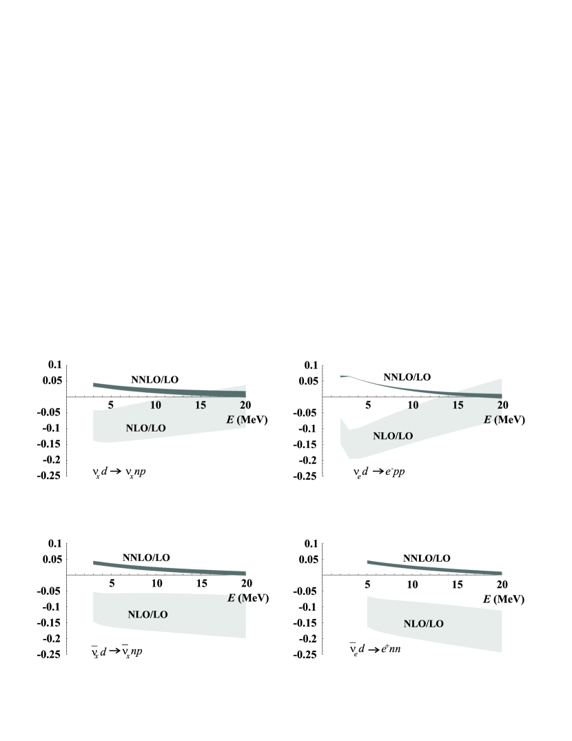
FIG. 8.: Testing convergence of the EFT calculation in each of the four channels studied. Shown are the relative NLO and NNLO contributions to the total cross-section in each channel, for values of $L_{1,A}$ between $-5~{}{\rm fm}^{3}$ and $+5~{}{\rm fm}^{3}$. Note that $\nu_{x}(\overline{\nu}_{x})$ represents $e,\ \mu,\ {\rm or}\tau$ neutrinos(antineutrinos).

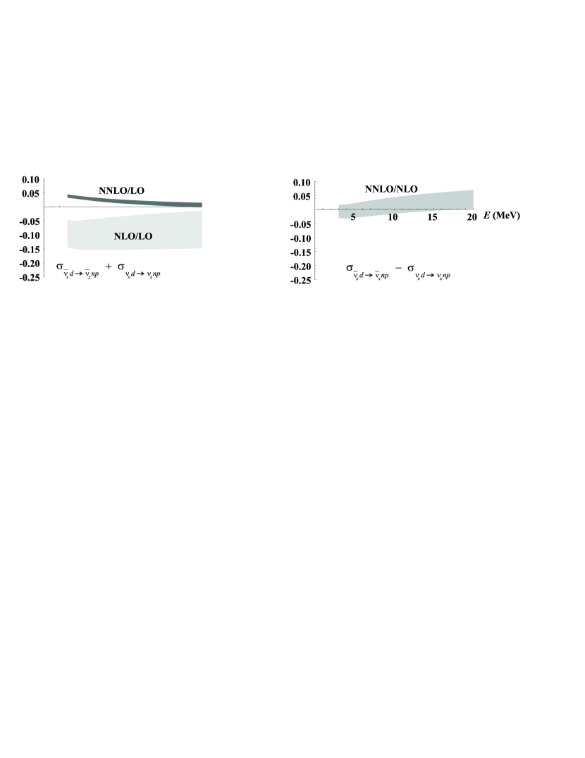
FIG. 9.: A further test of the convergence of the EFT calculation, using the NC channel. The left-hand graph arises from comparing contributions from the sum of the $\nu d$ and $\overline{\nu}d$ channels, or specifically the contributions from $W_{1}$ and $W_{2}$ which received contributions from all three orders of perturbation theory. The right-hand graph looks at the difference between the two channels, or specifically the contributions from $W_{3}$ which appear at NLO and NNLO only. As in fig 8, the shaded areas represent the effect of varying $L_{1,A}$ between $-5~{}{\rm fm}^{3}$ and $+5~{}{\rm fm}^{3}$.

	$\nu_{x}d\rightarrow\nu_{x}np$ ($x=e,\mu,\tau$)		$\overline{\nu}_{x}d\rightarrow\overline{\nu}_{x}np$ ($x=e,\mu,\tau$)
$E$ (MeV)	$a$ ($10^{-42}$ cm2)	$b$ ($10^{-42}$ cm2/fm3)	$a$ ($10^{-42}$ cm2)	$b$ ($10^{-42}$ cm2/fm3)
3	0.00315	0.000035	0.00312	0.000036
4	0.0287	0.00034	0.0282	0.00034
5	0.0885	0.0011	0.0865	0.0011
6	0.188	0.0024	0.182	0.0024
7	0.329	0.0044	0.318	0.0043
8	0.514	0.0070	0.49	0.0069
9	0.744	0.010	0.710	0.010
10	1.02	0.015	0.968	0.014
11	1.34	0.019	1.27	0.019
12	1.72	0.025	1.61	0.025
13	2.13	0.032	1.99	0.031
14	2.60	0.039	2.41	0.038
15	3.12	0.047	2.87	0.046
16	3.69	0.056	3.37	0.054
17	4.31	0.066	3.91	0.064
18	4.97	0.077	4.49	0.074
19	5.69	0.089	5.11	0.085
20	6.47	0.102	5.76	0.097

TABLE I.: Results for the neutral-current cross-sections, calculated to NNLO. The total cross-section for each channel is parameterized as $\sigma(E)=a(E)+b(E)L_{1,A}$.

	$\nu_{e}d\rightarrow e^{-}pp$		$\overline{\nu}_{e}d\rightarrow e^{+}nn$
$E$ (MeV)	$a$ ($10^{-42}$ cm2)	$b$ ($10^{-42}$ cm2/fm3)	$a$ ($10^{-42}$ cm2)	$b$ ($10^{-42}$ cm2/fm3)
2	0.00344	0.000031
3	0.0439	0.00044
4	0.146	0.0016
5	0.320	0.0036	0.0264	0.00030
6	0.574	0.0067	0.110	0.0014
7	0.914	0.011	0.261	0.0034
8	1.34	0.017	0.482	0.0065
9	1.87	0.024	0.776	0.011
10	2.48	0.032	1.14	0.016
11	3.20	0.042	1.58	0.023
12	4.01	0.054	2.09	0.032
13	4.93	0.067	2.68	0.041
14	5.95	0.082	3.33	0.052
15	7.08	0.098	4.06	0.065
16	8.31	0.12	4.85	0.079
17	9.66	0.14	5.71	0.094
18	11.12	0.16	6.63	0.11
19	12.70	0.18	7.63	0.13
20	14.39	0.21	8.68	0.15

TABLE II.: Results for the charged-current cross-sections calculated to NNLO. The total cross-section for each channel is parameterized as $\sigma(E)=a(E)+b(E)L_{1,A}$.

We compare our results to those of the potential model calculations NSGK  [12] and YHH [11] in fig. 10. We perform a global fit of our results to these model calculations with $L_{1,A}$ as the only free parameter. We find that the best fit to NSGK is given by $L_{1,A}^{NSGK}=5.6$ fm³, and for YHH $L_{1,A}^{YHH}=0.94$ fm³. These values are both consistent with the natural value of $L_{1,A}$ estimated in eq. (109) and the quality of the fit is impressive. This indicates the 5-10% difference in two potential model calculations is largely due to different assumptions made about short distance physics.

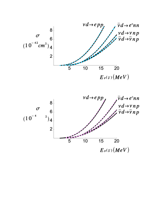
FIG. 10.: Inelastic $\nu(\overline{\nu})d$ cross-sections as a function of incident $\nu(\overline{\nu})$ energy. The solid curves in the upper graph are NSGK [12], while the dashed curves are the EFT results at NNLO, fit with $L_{1,A}=5.6$ fm³. The solid curves in the lower graph are the results of YHH  [11], and the dashed curves are the NNLO EFT results fit with $L_{1,A}=0.94$ fm³. In both graphs, the dashed curves all lie right on top of the solid curves.

We further examine the ratios of our cross-sections to the potential model results of NSGK and YHH in figs. 11 and 12 respectively. We see that there are deviations of order 5% between our result and YHH in all four channels. The fluctuations seen are in the results of YHH, and disagreements at threshold are most likely due to differences in the effective range parameters that can be associated with each calculation. However, the agreement between our result at NSGK is quite impressive - better than 1% over the whole range of neutrino energies studied. For comparison, we note the effective range parameters used here and those calculated from the potential used in NSGK [35] (using the Argonne $v_{18}$ potential [36], but with only Coulomb electromagnetic interactions) in table III.

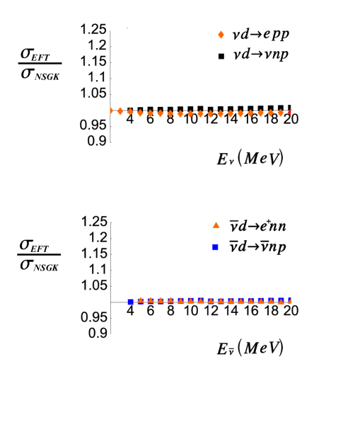
FIG. 11.: Ratios between the EFT calculation at NNLO and the potential model result of NSGK [12]. The upper graph compares the two channels of $\nu$-$d$ scattering, and the lower graph the two channels of $\overline{}\nu$-$d$ scattering. Agreement is better than 1% over the whole range of energies shown, for a single value of $L_{1,A}=5.6$ fm³.

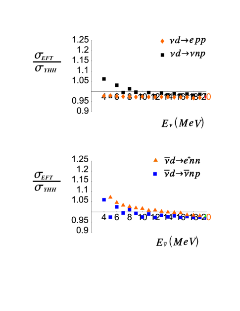
FIG. 12.: As in fig. 11, but comparing to the potential model result of YHH [11]. The agreement is not as good here, using a best-fit value of $L_{1,A}=0.94$ fm³.

	$a^{{}^{1}S_{0},pp}$ (fm)	$r^{{}^{1}S_{0},pp}_{0}$ (fm)	$a^{{}^{1}S_{0},nn}$ (fm)	$r^{{}^{1}S_{0},nn}_{0}$ (fm)	$a^{{}^{1}S_{0},np}$ (fm)	$r^{{}^{1}S_{0},np}_{0}$ (fm)	$\rho_{d}$ (fm)
This Work	-7.82	2.79	-18.5	2.80	-23.7	2.73	1.764
NSGK	-7.815	2.78	-18.5	2.83	-23.73	2.69	1.767

TABLE III.: Effective range parameters as used in our work and NSGK  [12].

Of import to SNO is the ratio between charged and neutral current cross-sections

$$R\equiv{\frac{\sigma_{CC}}{\sigma_{NC}}}\>.$$ (110)

As shown in ref. [13], this ratio $R$ at NLO was insensitive to the value of $L_{1,A}$, and that is still true at NNLO as seen in fig. 13. We consider two ratios, for both the $\nu$-$d$ (relevant to SNO) and $\overline{\nu}$-$d$ channels. The latter was the only channel discussed in ref.  [13]. Variations of $L_{1,A}$ over a large range, from $-20$ to $+40$ fm³, leads to a 6% variation in $R$. This likely represents an extreme variation, as it leads to as much as a 90% change in the total cross sections. The actual uncertainty in $R$ is almost certainly much less. Further, we can see that our values of $R$ agree well with the potential model results (fig. 14), with the worst agreement being seen when comparing to YHH. We use a median value of $L_{1,A}=3.7$ fm³ for this comparison. The poor agreement with YHH is biased towards threshold, and the likely reasons for this have already been discussed.

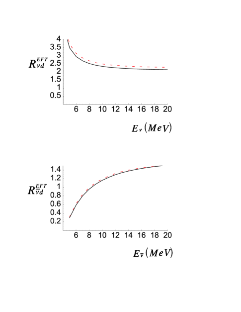
FIG. 13.: $CC$ to $NC$ cross-section ratios for $\nu-d$ and $\overline{\nu}-d$ scattering, as functions of incident energy. Shown are ratios of the EFT NNLO results with $L_{1,A}=-20$ fm³ (dashed) and $L_{1,A}=40$ fm³, demonstrating the insensitivity of the ratio to the value of $L_{1,A}$.

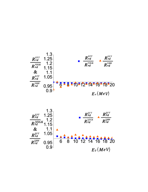
FIG. 14.: The ‘ratio of ratios’ between the EFT results at NNLO and those of NSGK [12] and YHH [11], with the EFT results using a median value of $L_{1,A}=3.7$ fm³. The upper graph compares the ratios for $\nu-d$ scattering, and the lower graph the ratios for $\overline{\nu}-d$ scattering. Again, the agreement with NSGK is excellent.

VI Summary and Conclusions

We have performed a calculation to NNLO of all four channels of $\nu d$ and $\overline{\nu}d$ breakup. Our work agrees very well with the latest potential model calculations, subject to the fitting of a single unknown counterterm $L_{1,A}$. Working at NNLO has allowed us to determine that our calculation indeed converges at the neutrino energies of interest, which in turn allows us to determine a formal theoretical uncertainty of 3% in our calculation. The only outstanding issue continues to be the determination of $L_{1,A}$.

It is imperative that an experimental determination of this counterterm be made. The theory without pions cannot reach energies that would allow this to be done with SAMPLE, but a breakthrough in the treatment of pions at NNLO might make access possible in the full theory. For now, ORLAND offers the best hope, with plans for a high-precision measurement in the $\nu$-$d$ CC channel.

ACKNOWLEDGMENTS

We would like to thank Martin Savage, Tom Cohen, John Beacom and Hamish Robertson for useful discussions. We would like to  thank K. Kubodera for providing us with the results of their new potential model calculation (NSGK) and T. Sato for providing information on that calculation’s effective range parameters. We thank the Department of Physics at the University of Washington where this work was initiated, the Institute for Nuclear Theory at the University of Washington for its hospitality and the Department of Energy for partial support during the completion of this work. J.-W.C. is supported, in part, by the Department of Energy under grant DOE/ER/40762-213. M.B. and X.K. are supported by grants from the Natural Sciences and Engineering Research Council of Canada.

A Fitting the Parameters of Effective Field Theory

Here, we summarize the fits to parameters in the theory without pions.

1 The ${}^{3}S_{1}$ channel

In the ${}^{3}S_{1}$ channel, we use the effective range expansion about the deuteron pole. Thus,

$$p\cot\delta_{0}=-\gamma+{\frac{1}{2}}\rho_{d}(p^{2}+\gamma^{2})+\ ...$$ (A1)

To keep the deuteron pole position unchanged at each order in perturbation theory, we expand

$$C_{0}^{(\,^{3}S_{1})} = C_{0,-1}^{(\,^{3}S_{1})}+C_{0,0}^{(\,^{3}S_{1})}+C_{0,1}^{(\,^{3}S_{1})}+\ ...$$ (A2)

$$C_{2}^{(\,^{3}S_{1})} = C_{2,-2}^{(\,^{3}S_{1})}+C_{2,-1}^{(\,^{3}S_{1})}+...$$ (A3)

$$C_{4}^{(\,^{3}S_{1})} = C_{4,-3}^{(\,^{3}S_{1})}+\ ...$$ (A4)

where the first index continues to denote the momentum dependence while the second index indicates the explicit power counting in the $Q$-expansion. Using the definition of the scattering amplitude

$${\cal A}={{\displaystyle{4\pi\over M_{N}}}}{\frac{1}{p\cot\delta_{0}-ip}}$$ (A5)

along with the amplitude computed using the power divergent subtraction (PDS) scheme proposed by KSW [14]

$${\cal A}_{EFE}=-{\frac{1}{{{\displaystyle{1\over C}}}+{{\displaystyle{M_{N}\over 4\pi}}}(\mu+ip)}}$$ (A6)

with $C=\sum C_{2n}^{(\,^{3}S_{1})}p^{2n}$.

Matching terms order-by-order in a $Q$-expansion, one obtains

$$C_{0,-1}^{(\,^{3}S_{1})} = {\frac{-4\pi}{M_{N}}}{\frac{1}{(\mu-\gamma)}}$$ (A7)

$$C_{0,0}^{(\,^{3}S_{1})} = {\frac{2\pi}{M_{N}}}{\frac{\rho_{d}\gamma^{2}}{(\mu-\gamma)^{2}}}$$ (A8)

$$C_{0,1}^{(\,^{3}S_{1})} = -{\frac{\pi}{M_{N}}}{\frac{\rho_{d}^{2}\gamma^{4}}{(\mu-\gamma)^{3}}}$$ (A9)

$$C_{2,-2}^{(\,^{3}S_{1})} = {\frac{2\pi}{M_{N}}}{\frac{\rho_{d}}{(\mu-\gamma)^{2}}}$$ (A10)

$$C_{2,-1}^{(\,^{3}S_{1})} = -{\frac{2\pi}{M_{N}}}{\frac{\rho_{d}^{2}\gamma^{2}}{(\mu-\gamma)^{3}}}$$ (A11)

$$C_{4,-3}^{(\,^{3}S_{1})} = -{\frac{\pi}{M_{N}}}{\frac{\rho_{d}^{2}}{(\mu-\gamma)^{3}}}\>,$$ (A12)

where we have neglected relativistic corrections.

2 The ${}^{1}S_{0}$ channel

We will deal with the $pp$ channel separately in the next section. For the $np$ and $nn$ channels, the procedure is somewhat simpler. The effective range expansion is given by

$$p\cot\delta_{0}=-{\frac{1}{a}}+{\frac{1}{2}}r_{0}p^{2}+\ ...$$ (A13)

Here, one obtains

$$C_{0}^{(\,^{1}S_{0})} = {\frac{-4\pi}{M_{N}}}{\frac{1}{\bigg{(}\mu-{{\displaystyle{1\over a^{(\,^{1}S_{0})}}}}\bigg{)}}}$$ (A14)

$$C_{2}^{(\,^{1}S_{0})} = {\frac{2\pi}{M_{N}}}{\frac{r_{0}^{(\,^{1}S_{0})}}{\bigg{(}\mu-{{\displaystyle{1\over a^{(\,^{1}S_{0})}}}}\bigg{)}^{2}}}$$ (A15)

$$C_{4}^{(\,^{1}S_{0})} = -{\frac{\pi}{M_{N}}}{\frac{r_{0}^{(\,^{1}S_{0})^{2}}}{\bigg{(}\mu-{{\displaystyle{1\over a^{(\,^{1}S_{0})}}}}\bigg{)}^{3}}}\>.$$ (A16)

3 The ${}^{1}S_{0}$ $pp$ channel

In this section we show how we fix the $pp$ scattering parameters to phase shift data through matching on to effective range expansion.

The S-wave $pp$ scattering amplitude can be decomposed into

$${\cal A}={\cal A}_{C}+{\cal A}_{SC}\qquad,$$ (A17)

where ${\cal A}_{C}$ is the pure Coulomb interaction amplitude with strong interaction “turned off” and ${\cal A}_{SC}$ is the remaining part with both strong and Coulomb interactions. Phase shifts $\delta$ and $\delta_{C}$ are defined by

$${\cal A} = \frac{4\pi}{M_{N}}\frac{e^{2i\delta}-1}{2ip}\qquad,$$ (A18)

$${\cal A}_{C} = \frac{4\pi}{M_{N}}\frac{e^{2i\delta_{C}}-1}{2ip}\qquad.$$ (A19)

Then

$${\cal A}_{SC}=\frac{4\pi}{M_{N}}e^{2i\delta_{C}}\left(\frac{e^{2i\delta_{SC}}-1}{2ip}\right)=\frac{4\pi}{M_{N}}\frac{e^{2i\delta_{C}}}{p\left(\cot\delta_{SC}-i\right)}\qquad,$$ (A20)

where $\delta_{SC}\equiv\delta-\delta_{C}.$ The Effective Range Expansion states that

$$p\left(\cot\delta_{SC}-i\right)=\left(-\frac{1}{a^{(pp)}}+\frac{1}{2}r_{0}^{(pp)}p^{2}+v^{(pp)}p^{4}+\cdots\right)-\alpha M_{N}H(\eta)\qquad,$$ (A21)

where $v^{(pp)}$ is the shape parameter. This expansion is related to ${\cal A}_{SC}/e^{2i\delta_{C}}$ which can be thought of as the $pp$ scattering amplitude with the pure Coulomb phase shift removed. The sum of the diagrams give

$$\frac{{\cal A}_{SC}}{e^{2i\delta_{C}}}\equiv A^{(1S_{0},pp)}=-{\displaystyle{1\over{\displaystyle{1\over C}}-J_{0}}}\qquad,$$ (A22)

where

$$C=\sum\limits_{n=0}^{\infty}C_{2n}^{(pp)}(p^{2}-\alpha M_{N}\mu)^{n}\qquad,$$ (A23)

and

$$J_{0}=\frac{\alpha M_{N}^{2}}{4\pi}\left(\ln\frac{\mu\sqrt{\pi}}{\alpha M_{N}}+1-\frac{3}{2}\gamma_{E}\right)-\frac{\mu M_{N}}{4\pi}-\frac{\alpha M_{N}^{2}}{4\pi}H(\eta)\qquad$$ (A24)

with the Euler’s constant $\gamma_{E}=0.577$. In eq. (A24), a 4-dimensional pole $\alpha M_{N}^{2}/(4\pi(4-d))$, along with the 3-dimensional pole, are subtracted from $J_{0}$ using the PDS prescription.

It is convenient to insert the expansion parameter $\varepsilon$ into eqs. (A20-A22) to keep track of the $Q$ expansion. Then the effective field theory parameters $C_{2n}^{(pp)}$ can be solved by matched on to the effective range expansion order-by-order in $\varepsilon$. The insertion of $\varepsilon$ is done by the transformation

$$\begin{array}[]{cc}{\displaystyle{1\over a^{(pp)}}}\rightarrow{\displaystyle{1\over a^{(pp)}}}\varepsilon&p\rightarrow p\varepsilon\\ r_{0}^{(pp)}\rightarrow r_{0}^{(pp)}&v^{(pp)}\rightarrow v^{(pp)}\\ \alpha M_{N}\rightarrow\alpha M_{N}\varepsilon^{2}&\mu\rightarrow\mu\varepsilon\\ H(\eta)\rightarrow H(\eta){\displaystyle{1\over\varepsilon}}&J_{0}\rightarrow J_{0}\varepsilon\end{array}$$ (A25)

The assignment of powers in $\varepsilon$ reflects the powers in $Q$ scaling of those parameters. For example, $1/a^{(pp)}$ and $p$ scale like $Q$, $\alpha M_{N}$ scales like $Q^{2}$ while $\left|H(\eta)\right|\leq p/(\alpha M_{N})$ scales like $1/\varepsilon$. The $C_{2n}^{(pp)}$ can be represented in a manner analogous that seen in the ${}^{3}S_{1}$ channel [19]

$$C_{0}^{(pp)} = C_{0,-1}^{(pp)}\varepsilon^{-1}+C_{0,0}^{(pp)}+C_{0,1}^{(pp)}\varepsilon+\cdots$$ (A26)

$$C_{2}^{(pp)} = C_{2,-2}^{(pp)}\varepsilon^{-2}+C_{2,-1}^{(pp)}\varepsilon^{-1}\ +\cdots$$ (A27)

$$C_{4}^{(pp)} = C_{4,-3}^{(pp)}\varepsilon^{-3}+\cdots\qquad.$$ (A28)

Then from  (A20-A22) we obtain

$$C_{0,-1}^{(pp)}=\frac{4\pi}{M_{N}}\frac{1}{{\displaystyle{1\over a^{(pp)}}}-\mu+\alpha M_{N}\left(\ln{\displaystyle{\mu\sqrt{\pi}\over\alpha M_{N}}}+1-\frac{3}{2}\gamma_{E}\right)}$$ (A29)

and

$$\begin{array}[t]{ll}C_{0,0}^{(pp)}=0&C_{0,1}^{(pp)}=\alpha M_{N}\mu C_{2,-2}^{(pp)}\\ C_{2,-2}^{(pp)}={\displaystyle{M_{N}\over 8\pi}}r_{0}^{(pp)}C_{0,-1}^{(pp)^{2}}&C_{2,-1}^{(pp)}=0\\ C_{4,-3}^{(pp)}={\displaystyle{M_{N}^{2}\over 64\pi^{2}}}r_{0}^{(pp)^{2}}C_{0,-1}^{(pp)^{3}}&\end{array}$$ (A30)

The solutions of parameters for $nn$ and $np^{(^{1}S_{0})}$ given in the previous section can be obtained by taking $\alpha=0$ from the above expressions.

B Summary of Scattering Cross Section

In this appendix, we explicitly list the relevant formulae for the four $\nu(\overline{\nu})d$ breakup processes. To make the formulae compact, certain higher order terms have been resummed. The $Q$-expansion expressions to NNLO shown in the text can always be recovered by expanding in $\epsilon$ to ${\cal O}(\epsilon^{2})$. Here $\epsilon$ is just a device to keep track of the $Q$-expansion – its value should be set to $1$ after the expansion is performed.

1 $\nu+d\rightarrow\nu+n+p$ and $\overline{\nu}+d\rightarrow\nu+n+p$

Differential cross section:

$${\displaystyle{d^{2}\sigma\over d\omega^{{}^{\prime}}d\Omega}}={\displaystyle{G_{F}^{2}\omega^{\prime}\left|{\bf k}^{\prime}\right|\over 2\pi^{2}}}\left[2W_{1}\sin^{2}{\displaystyle{\theta\over 2}}+W_{2}\cos^{2}{\displaystyle{\theta\over 2}}\mp 2{\displaystyle{(\omega+\omega^{\prime})\over M_{d}}}W_{3}\sin^{2}{\displaystyle{\theta\over 2}}\right]\quad,$$ (B1)

with $-(+)$ sign for the $\nu(\overline{\nu})d$ scattering.

Phase space:

$$\text{Max}\left[-1,1-{\displaystyle{4M_{N}(\nu-B)-\nu^{2}\over 2\omega\omega^{\prime}}}\right]\leq\cos\theta\leq 1\quad,$$ (B2)

$$0\leq\omega^{\prime}\leq\omega-2(M_{N}-\sqrt{M_{N}^{2}-\gamma^{2}})\quad.$$ (B3)

Structure functions (as mentioned above, one can obtain the NNLO results by expanding $\epsilon$ to ${\cal O}(\epsilon^{2})$ ):

$$W_{1} = \frac{1}{\left(1-\epsilon\gamma\rho_{d}\right)}\left[2(C_{A}^{(0)^{2}}+C_{A}^{(1)^{2}})F_{1}+{\displaystyle{1\over 3}}(C_{A}^{(0)^{2}}-C_{A}^{(1)^{2}})F_{2}+\frac{8}{3}C_{A}^{(0)^{2}}F_{3}+\frac{4}{3}C_{A}^{(1)^{2}}F_{4}+G_{2}\right]\quad,$$ (B4)

$$W_{2} = W_{1}+\frac{1}{\left(1-\epsilon\gamma\rho_{d}\right)}\left[2(C_{V}^{(0)^{2}}+C_{V}^{(1)^{2}})F_{1}+(C_{V}^{(0)^{2}}-C_{V}^{(1)^{2}})F_{2}+4C_{V}^{(0)^{2}}F_{3}+G_{1}\right]\quad,$$ (B5)

$$W_{3} = \frac{-2\epsilon}{\left(1-\epsilon\gamma\rho_{d}\right)}\left[2(C_{A}^{(0)}C_{M}^{(0)}+C_{A}^{(1)}C_{M}^{(1)})F_{1}+{\displaystyle{1\over 3}}(C_{A}^{(0)}C_{M}^{(0)}-C_{A}^{(1)}C_{M}^{(1)})F_{2}+\frac{8}{3}C_{A}^{(0)}C_{M}^{(0)}F_{3}\right.$$ (B7)

$$\left.+\frac{4}{3}C_{A}^{(1)}C_{M}^{(1)}F_{4}+G_{3}\right]$$

$$\begin{array}[t]{ll}C_{V}^{(0)}=-\sin^{2}\vartheta_{W}&,\quad C_{V}^{(1)}={\displaystyle{1\over 2}}(1-2\sin^{2}\vartheta_{W})\quad,\\ C_{A}^{(0)}=-{\displaystyle{1\over 2}}\Delta s&,\quad C_{A}^{(1)}={\displaystyle{1\over 2}}g_{A}\quad,\\ C_{M}^{(0)}=-2\sin^{2}\vartheta_{W}\kappa^{(0)}-\frac{1}{2}\mu_{S}&,\quad C_{M}^{(1)}=(1-2\sin^{2}\vartheta_{W})\kappa^{(1)}\quad.\end{array}$$ (B8)

$$F_{1} = {\displaystyle{2M_{N}\gamma\ p\over\pi\left(p^{2}+\gamma^{2}\right)^{2}}}\left(1+\frac{{\bf q}^{2}\left(p^{2}-\gamma^{2}\right)}{2\left(p^{2}+\gamma^{2}\right)^{2}}\right)\quad,\quad F_{2}={\displaystyle{4M_{N}\gamma\ p\over\pi\left(p^{2}+\gamma^{2}\right)^{2}}}\left(1-\frac{{\bf q}^{2}\left(p^{2}+3\gamma^{2}\right)}{6\left(p^{2}+\gamma^{2}\right)^{2}}\right)\quad,$$ (B9)

$$F_{3} = {\displaystyle{1\ \over\pi}}\text{Im}\left[B_{0}{}^{2}\left(A_{-1}^{(^{3}S_{1})}(p)+\epsilon A_{0}^{(^{3}S_{1})}(p)+\epsilon^{2}A_{1}^{(^{3}S_{1})}(p)\right)\right]\quad,$$ (B10)

$$F_{4} = F_{3}(^{3}S_{1}\rightarrow\ ^{1}S_{0},np)\ \quad.$$ (B11)

$$B_{0}={\bf-}\sqrt{\frac{\gamma}{2\pi}}\frac{M_{N}}{\gamma-ip}\left(1-\frac{{\bf q}^{2}}{12\left(\gamma-ip\right)^{2}}\right)$$ (B12)

$$p=\sqrt{M_{N}\nu-\gamma^{2}-\frac{{\bf q}^{2}}{4}+i\epsilon}\quad,$$ (B13)

$$G_{1} = \epsilon C_{V}^{(0)^{2}}{\displaystyle{2M_{N}\rho_{d}\over\pi}}\mathop{\rm Im}\left[\sqrt{\frac{2\gamma}{\pi}}B_{0}\left(A_{-1}^{(^{3}S_{1})}(p)+\epsilon A_{0}^{(^{3}S_{1})}(p)\right)\right]\quad,$$ (B14)

$$G_{2} = -\epsilon{\displaystyle{M_{N}\over 3\pi^{2}}}\mathop{\rm Im}\left[\sqrt{\frac{\gamma}{2\pi}}B_{0}\left[C_{A}^{(1)}\widetilde{L}_{1,A}\left(A_{-1}^{(^{1}S_{0},np)}(p)+\epsilon A_{0}^{(^{1}S_{0},np)}(p)\right)+4C_{A}^{(0)}\widetilde{L}_{2,A}\left(A_{-1}^{(^{3}S_{1})}(p)+\epsilon A_{0}^{(^{3}S_{1})}(p)\right)\right]\right]$$ (B16)

$$+\epsilon^{2}{\displaystyle{M_{N}^{2}\gamma\over 96\pi^{4}}}\mathop{\rm Im}\left[\left(\widetilde{L}_{1,A}^{2}A_{-1}^{(^{1}S_{0},np)}(p)+8\widetilde{L}_{2,A}^{2}A_{-1}^{(^{3}S_{1})}(p)\right)\right]\quad,$$

$$G_{3} = \epsilon^{2}{\displaystyle{M_{N}\over 3\pi^{2}}}\mathop{\rm Im}\left\{\sqrt{\frac{\gamma}{2\pi}}B_{0}(p,\left|{\bf q}\right|{\bf)}\left[\left(C_{M}^{(1)}\widetilde{L}_{1,A}+C_{A}^{(1)}\widetilde{L}_{1,M}\ \right)A_{-1}^{(^{1}S_{0},np)}(p)\right.\right.$$ (B18)

$$\left.\left.+4\left(C_{M}^{(0)}\widetilde{L}_{2,A}+C_{A}^{(0)}\widetilde{L}_{2,M}\right)A_{-1}^{(^{3}S_{1})}(p)\right]\right\}$$

$$\widetilde{L}_{1,A} = -\frac{4\pi\left(\mu-\gamma\right)}{M_{N}C_{0}^{(^{1}S_{0},np)}}\left[L_{1,A}-2\pi C_{A}^{(1)}\left(\frac{M_{N}}{2\pi}C_{2}^{(^{1}S_{0},np)}+\frac{\rho_{d}}{\left(\mu-\gamma\right)^{2}}\right)\right]\quad,$$ (B19)

$$\widetilde{L}_{2,A} = \left(\mu-\gamma\right)^{2}L_{2,A}-2\pi C_{A}^{(0)}\rho_{d}\quad.$$ (B20)

$$\widetilde{L}_{1,M} = -\frac{8\pi\left(\mu-\gamma\right)}{M_{N}C_{0}^{(^{1}S_{0},np)}}\left[(1-2\sin^{2}\vartheta_{W})M_{N}L_{1}-\pi C_{M}^{(1)}\left(\frac{M_{N}}{2\pi}C_{2}^{(^{1}S_{0},np)}+\frac{\rho_{d}}{\left(\mu-\gamma\right)^{2}}\right)\right]\quad,$$ (B21)

$$\widetilde{L}_{2,M} = \ -4\sin^{2}\vartheta_{W}\left(\mu-\gamma\right)^{2}M_{N}L_{2}-2\pi C_{M}^{(0)}\rho_{d}\quad,$$ (B22)

evaluated at $\mu=m_{\pi}$, with $C_{0}^{(\,^{1}S_{0},np)}=-3.56$ fm² and $C_{2}^{(\,^{1}S_{0},np)}=6.55$ fm⁴. Further, $\Delta s=-0.17$, and $\mu_{s}=L_{2,A}=0$ are used in our calculation (though the results are not sensitive to these choices).

2 $\overline{\nu}+d\rightarrow e^{+}+n+n$

Differential cross section:

$${\displaystyle{d^{2}\sigma\over d\omega^{{}^{\prime}}d\Omega}}={\displaystyle{G_{F}^{2}\omega^{\prime}\left|{\bf k}^{\prime}\right|\over 2\pi^{2}}}\left[2W_{1}\sin^{2}{\displaystyle{\theta\over 2}}+W_{2}\cos^{2}{\displaystyle{\theta\over 2}}+2{\displaystyle{(\omega+\omega^{\prime})\over M_{d}}}W_{3}\sin^{2}{\displaystyle{\theta\over 2}}\right]\quad,$$ (B23)

Phase space:

$$\text{Max}\left[-1,-{\displaystyle{\frac{4M_{N}(\nu-B+m_{n}-m_{p})-\omega^{2}-\omega^{\prime 2}+m_{e}^{2}}{2\omega\sqrt{\omega^{\prime 2}-m_{e}^{2}}\ }}}\right]\leq\cos\theta\leq 1\quad,$$ (B24)

$$m_{e}\leq\omega^{\prime}\leq\omega-2(M_{N}-\sqrt{M_{N}^{2}-M_{N}(B-m_{n}+m_{p})})$$ (B25)

Structure functions:

$$W_{1} = \frac{1}{\left(1-\epsilon\gamma\rho_{d}\right)}\left[2C_{A}^{(1)^{2}}F_{1}-{\displaystyle{1\over 3}}C_{A}^{(1)^{2}}F_{2}+\frac{4}{3}C_{A}^{(1)^{2}}F_{4}+G_{2}\right]\quad,$$ (B26)

$$W_{2} = W_{1}+\frac{1}{\left(1-\epsilon\gamma\rho_{d}\right)}\left[2C_{V}^{(1)^{2}}F_{1}-C_{V}^{(1)^{2}}F_{2}\right]\quad,$$ (B27)

$$W_{3} = \frac{-2\epsilon}{\left(1-\epsilon\gamma\rho_{d}\right)}\left[2C_{A}^{(1)}C_{M}^{(1)}F_{1}-{\displaystyle{1\over 3}}C_{A}^{(1)}C_{M}^{(1)}F_{2}+\frac{4}{3}C_{A}^{(1)}C_{M}^{(1)}F_{4}+G_{3}\right]\quad.$$ (B28)

$$p=\sqrt{M_{N}\left(\nu+m_{n}-m_{p}\right)-\gamma^{2}-\frac{{\bf q}^{2}}{4}+i\epsilon}\quad,$$ (B29)

$$C_{V}^{(1)}={\displaystyle{\left|V_{ud}\right|\over\sqrt{2}}}\quad,\quad C_{A}^{(1)}={\displaystyle{\left|V_{ud}\right|\over\sqrt{2}}}g_{A}\quad,\quad C_{M}^{(1)}=\sqrt{2}\left|V_{ud}\right|\kappa^{(1)}\quad$$ (B30)

$$F_{1} = {\displaystyle{2M_{N}\gamma\ p\over\pi\left(p^{2}+\gamma^{2}\right)^{2}}}\left(1+\frac{{\bf q}^{2}\left(p^{2}-\gamma^{2}\right)}{2\left(p^{2}+\gamma^{2}\right)^{2}}\right)\quad,\quad F_{2}={\displaystyle{4M_{N}\gamma\ p\over\pi\left(p^{2}+\gamma^{2}\right)^{2}}}\left(1-\frac{{\bf q}^{2}\left(p^{2}+3\gamma^{2}\right)}{6\left(p^{2}+\gamma^{2}\right)^{2}}\right)\quad,$$ (B31)

$$F_{4} = {\displaystyle{1\ \over\pi}}\text{Im}\left[B_{0}{}^{2}\left(A_{-1}^{(^{1}S_{0},nn)}(p)+\epsilon A_{0}^{(^{1}S_{0},nn)}(p)+\epsilon^{2}A_{1}^{(^{1}S_{0},nn)}(p)\right)\right]\ \quad.$$ (B32)

$$G_{2} = -\epsilon{\displaystyle{M_{N}\over 3\pi^{2}}}\mathop{\rm Im}\left[\sqrt{\frac{\gamma}{2\pi}}B_{0}C_{A}^{(1)}\widetilde{L}_{1,A}\left(A_{-1}^{(^{1}S_{0},nn)}(p)+\epsilon A_{0}^{(^{1}S_{0},nn)}(p)\right)\right]$$ (B34)

$$+\epsilon^{2}{\displaystyle{M_{N}^{2}\gamma\over 96\pi^{4}}}\mathop{\rm Im}\left[\widetilde{L}_{1,A}^{2}A_{-1}^{(^{1}S_{0},nn)}(p)\right]\quad,$$

$$G_{3} = \epsilon^{2}{\displaystyle{M_{N}\over 3\pi^{2}}}\mathop{\rm Im}\left[\sqrt{\frac{\gamma}{2\pi}}B_{0}\left(C_{M}^{(1)}\widetilde{L}_{1,A}+C_{A}^{(1)}\widetilde{L}_{1,M}\ \right)A_{-1}^{(^{1}S_{0},nn)}(p)\right]\quad.$$ (B35)

$$\widetilde{L}_{1,A} = -\frac{4\pi\left(\mu-\gamma\right)}{M_{N}C_{0}^{(^{1}S_{0},nn)}}\left[\sqrt{2}\left|V_{ud}\right|L_{1,A}-2\pi C_{A}^{(1)}\left(\frac{M_{N}}{2\pi}C_{2}^{(^{1}S_{0},nn)}+\frac{\rho_{d}}{\left(\mu-\gamma\right)^{2}}\right)\right]\quad,$$ (B36)

$$\widetilde{L}_{1,M} = -\frac{8\pi\left(\mu-\gamma\right)}{M_{N}C_{0}^{(^{1}S_{0},nn)}}\left[\sqrt{2}\left|V_{ud}\right|M_{N}L_{1}-\pi C_{M}^{(1)}\left(\frac{M_{N}}{2\pi}C_{2}^{(^{1}S_{0},nn)}+\frac{\rho_{d}}{\left(\mu-\gamma\right)^{2}}\right)\right]\quad,$$ (B37)

evaluated at $\mu=m_{\pi}$, with $C_{0}^{(\,^{1}S_{0},nn)}=-3.49$ fm² and $C_{2}^{(\,^{1}S_{0},nn)}=6.46$ fm⁴.

3 $\nu_{e}+d\rightarrow e^{-}+p+p$

Differential cross section:

$${\displaystyle{d^{2}\sigma\over d\omega^{{}^{\prime}}d\Omega}} = {\displaystyle{G_{F}^{2}\omega^{\prime}\left|{\bf k}^{\prime}\right|\over 2\pi^{2}}}\frac{2\pi\eta_{e}}{1-e^{-2\pi\eta_{e}\eta_{e}}\ }\left[2W_{1}\sin^{2}{\displaystyle{\theta\over 2}}+W_{2}\cos^{2}{\displaystyle{\theta\over 2}}-2{\displaystyle{(\omega+\omega^{\prime})\over M_{d}}}W_{3}\sin^{2}{\displaystyle{\theta\over 2}}\right]\quad,$$ (B38)

$$\eta_{e} = \frac{2\alpha\omega^{\prime}}{\left|{\bf k}^{\prime}\right|}\quad.$$ (B39)

Phase space:

$$\text{Max}\left[-1,-{\displaystyle{\frac{4M_{N}(\nu-B+m_{n}-m_{p})-\omega^{2}-\omega^{\prime 2}+m_{e}^{2}}{2\omega\sqrt{\omega^{\prime 2}-m_{e}^{2}}\ }}}\right]\leq\cos\theta\leq 1\quad,$$ (B40)

$$m_{e}\leq\omega^{\prime}\leq\omega-2(M_{N}-\sqrt{M_{N}^{2}-M_{N}(B-m_{n}+m_{p})})$$ (B41)

Structure functions:

$$W_{1} = \frac{1}{\left(1-\epsilon\gamma\rho_{d}\right)}\left[2C_{A}^{(1)^{2}}F_{1}-{\displaystyle{1\over 3}}C_{A}^{(1)^{2}}F_{2}+\frac{4}{3}C_{A}^{(1)^{2}}F_{4}+G_{2}\right]\quad,$$ (B42)

$$W_{2} = W_{1}+\frac{1}{\left(1-\epsilon\gamma\rho_{d}\right)}\left[2C_{V}^{(1)^{2}}F_{1}-C_{V}^{(1)^{2}}F_{2}\right]\quad,$$ (B43)

$$W_{3} = \frac{-2\epsilon}{\left(1-\epsilon\gamma\rho_{d}\right)}\left[2C_{A}^{(1)}C_{M}^{(1)}F_{1}-{\displaystyle{1\over 3}}C_{A}^{(1)}C_{M}^{(1)}F_{2}+\frac{4}{3}C_{A}^{(1)}C_{M}^{(1)}F_{4}+G_{3}\right]\quad.$$ (B44)

$$F_{1} = {\displaystyle{2M_{N}\gamma\ p\over\pi\left(p^{2}+\gamma^{2}\right)^{2}}}\left(1+\frac{{\bf q}^{2}\left(p^{2}-\gamma^{2}-2\eta p\gamma\right)}{2\left(p^{2}+\gamma^{2}\right)^{2}}\right)\left({\displaystyle{2\pi\eta\over\ e^{2\pi\eta}-1\ }}\right)e^{4\eta\tan^{-1}\left(\frac{p}{\gamma}\right)}\quad,$$ (B45)

$$\quad F_{2} = {\displaystyle{4M_{N}\gamma\ p\over\pi\left(p^{2}+\gamma^{2}\right)^{2}}}\left(1-\frac{{\bf q}^{2}\left(p^{2}+3\gamma^{2}+6\eta p\gamma\right)}{6\left(p^{2}+\gamma^{2}\right)^{2}}\right)\left({\displaystyle{2\pi\eta\over\ e^{2\pi\eta}-1\ }}\right)e^{4\eta\tan^{-1}\left(\frac{p}{\gamma}\right)}\quad\quad,$$ (B46)

$$F_{4} = {\displaystyle{1\ \over\pi}}\text{Im}\left[B_{0}{}^{2}\left(A_{-1}^{(^{1}S_{0},pp)}(p)+\epsilon A_{0}^{(^{1}S_{0},pp)}(p)+\epsilon^{2}A_{1}^{(^{1}S_{0},pp)}(p)\right)\right]\quad,$$ (B47)

$$B_{0} = M_{N}\int\frac{d^{3}k}{\left(2\pi\right)^{3}}\frac{\sqrt{8\pi\gamma}}{k^{2}+\gamma^{2}}{\displaystyle{2\pi\eta_{k}\over e^{2\pi\eta_{k}}-1\ }}\frac{e^{2\eta_{k}\tan^{-1}\left(\frac{k}{\gamma}\right)}}{p^{2}-k^{2}+i\epsilon}$$ (B49)

$$\qquad\qquad\qquad\qquad\left[1+\frac{{\bf q}^{2}\left(\left(1-2\eta_{k}^{2}\right)k^{2}-6\eta_{k}k\gamma-3\gamma^{2}\right)}{12\left(q^{2}+\gamma^{2}\right)^{2}}\right]\quad,$$

$$\eta = \frac{\alpha M_{N}}{2p}\quad,\quad\eta_{k}=\frac{\alpha M_{N}}{2k}\quad.$$ (B50)

$$p=\sqrt{M_{N}\left(\nu-m_{n}+m_{p}\right)-\gamma^{2}-\frac{{\bf q}^{2}}{4}+i\epsilon}\quad,$$ (B51)

$\displaystyle C_{V}^{(1)}={\displaystyle{\left|V_{ud}\right|\over\sqrt{2}}}\quad,\quad C_{A}^{(1)}={\displaystyle{\left|V_{ud}\right|\over\sqrt{2}}}g_{A}\quad,\quad C_{M}^{(1)}=\sqrt{2}\left|V_{ud}\right|\kappa^{(1)}\quad$

$$G_{2} = -\epsilon{\displaystyle{M_{N}\over 3\pi^{2}}}\mathop{\rm Im}\left[\sqrt{\frac{\gamma}{2\pi}}B_{0}C_{A}^{(1)}\widetilde{L}_{1,A}\left(A_{-1}^{(^{1}S_{0},pp)}(p)+\epsilon A_{0}^{(^{1}S_{0},pp)}(p)\right)\right]$$ (B53)

$$+\epsilon^{2}{\displaystyle{M_{N}^{2}\gamma\over 96\pi^{4}}}\mathop{\rm Im}\left[\widetilde{L}_{1,A}^{2}A_{-1}^{(^{1}S_{0},pp)}(p)\right]\quad,$$

$$G_{3} = \epsilon^{2}{\displaystyle{M_{N}\over 3\pi^{2}}}\mathop{\rm Im}\left[\sqrt{\frac{\gamma}{2\pi}}B_{0}\left(C_{M}^{(1)}\widetilde{L}_{1,A}+C_{A}^{(1)}\widetilde{L}_{1,M}\ \right)A_{-1}^{(^{1}S_{0},pp)}(p)\right]\quad.$$ (B54)

$$\widetilde{L}_{1,A} = -\frac{4\pi\left(\mu-\gamma\right)}{M_{N}C_{0}^{(^{1}S_{0},pp)}}\left[\sqrt{2}\left|V_{ud}\right|L_{1,A}-2\pi C_{A}^{(1)}\left(\frac{M_{N}}{2\pi}C_{2}^{(^{1}S_{0},pp)}+\frac{\rho_{d}}{\left(\mu-\gamma\right)^{2}}\right)\right]\quad,$$ (B55)

$$\widetilde{L}_{1,M} = -\frac{8\pi\left(\mu-\gamma\right)}{M_{N}C_{0}^{(^{1}S_{0},pp)}}\left[\sqrt{2}\left|V_{ud}\right|M_{N}L_{1}-\pi C_{M}^{(1)}\left(\frac{M_{N}}{2\pi}C_{2}^{(^{1}S_{0},pp)}+\frac{\rho_{d}}{\left(\mu-\gamma\right)^{2}}\right)\right]\quad,$$ (B56)

evaluated at $\mu=m_{\pi}$, with $C_{0}^{(\,^{1}S_{0},pp)}=-3.77$ fm² and $C_{2}^{(\,^{1}S_{0},pp)}=7.50$ fm⁴.

REFERENCES

- [1] G.T. Ewan et al., SNO proposal SNO-87-12, 1987.
- [2] G.A. Aardsma et al., Phys. Lett. B 194, 321 (1987).
- [3] F.T. Avignone and Yu.V. Efremenko, in Proceedings of the 2000 Carolina Conference on Neutrino Physics, Ed. K. Kubodera (World Scientific, 2000) in press.
- [4] S.D. Ellis and J.N. Bahcall, Nucl. Phys. A 114, 636 (1968).
- [5] A. Ali and C.A. Dominguez, Phys. Rev. D 12, 3673 (1975).
- [6] H. C. Lee, Nucl. Phys. A 294, 473 (1978).
- [7] J.N. Bahcall, K. Kubodera, and S. Nozawa, Phys. Rev. D 38, 1030 (1987).
- [8] N. Tatara, Y. Kohyama and K. Kubodera, Phys. Rev. C 42, 1694 (1990).
- [9] M. Doi and K. Kubodera, Phys. Rev. C 45, 1988 (1992).
- [10] K. Kubodera and S. Nozawa, Int. J. Mod. Phys. E3, 101 (1994); Y. Kohyama and K. Kubodera, USC(NT)-Report-92-1, 1992, unpublished.
- [11] S. Ying, W.C. Haxton, and E. M. Henley, Phys. Rev. C 45, 1982 (1992); Phys. Rev. D 40, 3211 (1989).
- [12] S. Nakamura, T. Sato, V. Gudkov, and K. Kubodera, in preparation.
- [13] M.N. Butler and J.W. Chen, Nucl. Phys. A675, 575 (2000).
- [14] D.B. Kaplan, M.J. Savage and M.B. Wise, Phys. Lett. B 424, 390 (1998); Nucl. Phys. B 534, 329 (1998); Phys.Rev. C59, 617 (1999).
- [15] T.D. Cohen and J.M. Hansen, Phys. Rev. C59, 13 (1999).
- [16] G. Rupak and N. Shoresh, Phys. Rev. C60, 054004 (1999).
- [17] D.B. Kaplan and J.V. Steele, Phys. Rev. C60, 064002 (1999).
- [18] S. Fleming , T. Mehen and I. W. Stewart,Phys. Rev. C61, 044005 (2000); Nucl. Phys. A677, 313 (2000).
- [19] J.W. Chen, G. Rupak and M.J. Savage, Nucl. Phys. A653, 386 (1999).
- [20] D.B. Kaplan, M.J. Savage and M.B. Wise, Nucl. Phys. B478, 629 (1996).
- [21] D.B. Kaplan, Nucl. Phys. B494, 471 (1997).
- [22] T.D. Cohen, Phys. Rev. C55, 67 (1997); D.R. Phillips and T.D. Cohen, Phys. Lett. B390, 7 (1997); S.R. Beane, T.D. Cohen, and D.R. Phillips, Nucl. Phys. A632, 445 (1998).
- [23] M. Luke and A. Manohar, Phys. Rev. D55, 4129 (1997).
- [24] G.P. Lepage, nucl-th/9706029.
- [25] U. van Kolck, hep-ph/9711222; Nucl. Phys. A645 273 (1999).
- [26] P.F. Bedaque and U. van Kolck, Phys. Lett. B428, 221 (1998); P.F. Bedaque, H.W. Hammer, and U. van Kolck, Phys. Rev. Lett. 82, 463 (1999).
- [27] J.W. Chen and M.J. Savage, Phys. Rev. C60, 065205 (1999); J.W. Chen, G. Rupak and M.J. Savage, Phys. Lett. B464, 1 (1999).
- [28] G. Rupak, nucl-th/9911018.
- [29] X. Kong and F. Ravndal, Phys. Lett. B450, 320 (1999); Nucl. Phys. A656, 421 (1999); Nucl. Phys. A665, 137 (2000); nucl-th/0004038.
- [30] M.J.Savage and J. Walden, Phys. Rev. D55, 5376 (1997).
- [31] D.B. Kaplan and A. Manohar, Nucl. Phys. B310, 527 (1988).
- [32] B. Mueller et al., Phys. Rev. Lett. 78, 3824 (1997).
- [33] M. Pitt, private communication.
- [34] G. A. Miller, W.T.H. Van Oers, in ‘Symmetries and fundamental interactions in nuclei’ edited by W.C. Haxton and E.M. Henley, nucl-th/9409013.
- [35] T. Sato, S. Nakamura, and K. Kubodera, private communication.
- [36] R.B. Wiringa, V.G.J. Stoks, and R. Schiavilla, Phys. Rev. C51, 38 (1995).