Anti-Kaon Induced Reactions on the Nucleon

Abstract

Using a previously established effective Lagrangian model we describe anti-kaon induced reactions on the nucleon. The dominantly contributing channels in the cm-energy region from threshold up to 1.72 GeV are included ($\overline{K}N$, $\pi\Sigma$, $\pi\Lambda$). We solve the Bethe-Salpeter equation in an unitary $K$-matrix approximation.

I Introduction

One major goal in hadron physics is to find the properties of resonances. In the sector of $N^{*}$ and $\Delta$ resonances there exists a huge amount of data especially from $\pi N$ reactions. The properties of most of these resonances are known quite well [1] from various analyses of the experimental data (see for example [2]) and models that are able to describe these data, as for example [3]. This situation changes when we look at resonances with strangeness $-1$. Here the properties of some resonances are not settled at all (e.g. in the $P_{01}$ partial wave there might be one or two resonances with barely known masses and widths). In order to learn more about these resonances and also the coupling constants involving strange baryons, we have extended the model of [3] to the strangeness $-1$ sector (i.e. the asymptotic states are $\overline{K}N$, $\pi\Sigma$, and $\pi\Lambda$).

Reference [3] sets the framework of the present calculation. Using the $K$ matrix approximation, $\pi$ and $\gamma$ induced reactions on the nucleon with final states $\pi N$, $\gamma N$, $\pi\pi N$, $\eta N$, $K\Lambda$, and since last year also $K\Sigma$, were calculated. Also on the basis of [3] Bennhold et al. [4] are investigating nucleon and $\Delta$ resonances. In their latest publication [5], special emphasis is put on the photoproduction of kaon hyperon states. Especially with the inclusion of the final state $K\Sigma$ it was possible to extend the energy range up to $\sqrt{s}=2$ GeV and thus to investigate the resonances around 1900 MeV. For the photoproduction it is very important to maintain gauge invariance after introducing form factors. Using a form factor prescription by Haberzettl [6] yields an excellent agreement between experimental data and model calculations.

In general, experimental observables are very well described with the model in [3]; however, there is a problem concerning the final states $K\Lambda$ and $K\Sigma$; the angular differential cross sections for the $\pi$ induced reactions do not agree with experiment. In the reactions $\pi N\rightarrow K\Lambda$ or $K\Sigma$ there are baryons and resonances with strangeness $-1$ propagating in $u$-channel diagrams. Since these are nonresonant contributions and the couplings of the baryons and widths of the resonances are, if at all, poorly known, these diagrams were not included in [3].

The idea is now to determine these parameters in a calculation where they contribute in resonant diagrams, which is the case for $\overline{K}$ induced reactions on the nucleon.

In this paper we present our first results. Section II shows the concept of our calculation with the unitarity conserving $K$ matrix approximation, which reduces the Bethe-Salpeter equation from a system of coupled integral equations to the problem of matrix inversion. Section III covers the used Lagrange density and motivates the final states that have to be considered in the calculation. In section III A the used form factors are given and in the following section IV the experimental data that were used for the fit are discussed. Our results are presented in section V. Section VI contains conclusions and outlook.

II The Model

All information of the scattering process is contained in the scattering matrix $S$. This matrix can be decomposed into a trivial part and the part that includes all information about reactions, the $T$-matrix

$$S=I+{\rm i}\;T.$$ (1)

The scattering equation that needs to be solved is the Bethe Salpeter equation (BSE). Schematically the BSE is given as illustrated in fig. 1. $V$ is the amplitude of the elementary interactions and is calculated using Feynman rules which follow from a Lagrangian that is given in section III. The two-particle propagator $\mathcal{G}_{BS}$ is given by the product of the baryon and the meson propagator. The integration over the loop momentum yields a system of coupled integral equations for all final states.

We introduce the Feynman amplitude $\mathcal{M}$

$$\langle\mbox{\boldmath$\displaystyle p$}_{1}\mbox{\boldmath$\displaystyle p$}_{2}|{\rm i}\hat{T}|\mbox{\boldmath$\displaystyle k$}_{A}\mbox{\boldmath$\displaystyle k$}_{B}\rangle=(2\pi)^{4}\delta^{(4)}(k_{A}+k_{B}-(p_{1}+p_{2})){\rm i}{\mathcal{M}}(k_{A},k_{B}\rightarrow p_{1},p_{2}).$$ (2)

Taking out the spinors we define the amplitude $M_{fi}$

$${\cal M}_{fi}=\bar{u}(p^{\prime},s^{\prime})M_{fi}u(p,s).$$ (3)

Then the BSE has the form

$$M(p^{\prime},p;\sqrt{s})=V(p^{\prime},p;\sqrt{s})+\int\frac{d^{4}k}{(2\pi)^{4}}V(p^{\prime},k;\sqrt{s})\;{\cal G}_{BS}(k;\sqrt{s})\;M(k,p,\sqrt{s}).$$ (4)

To make this problem solvable we are using a $K$ matrix approximation. In our notation the $K$ matrix is defined by

$$K = V(p^{\prime},p;\sqrt{s})+{\mathrm{P}}\int\frac{d^{4}k}{(2\pi)^{4}}V(p^{\prime},k;\sqrt{s})\;{\cal G}_{BS}(k;\sqrt{s})\;K(k,p,\sqrt{s})$$ (5)

$$= V(p^{\prime},p;\sqrt{s})+\int\frac{d^{4}k}{(2\pi)^{4}}V(p^{\prime},k;\sqrt{s})\;\Re{\cal G}_{BS}(k;\sqrt{s})\;K(k,p,\sqrt{s}),$$ (6)

where P stands for the principal value of the integral and $\Re{\cal G}_{BS}$ stands for the real part of the propagator. The latter contains the pole of the propagator as can be seen from the following. A propagator is given in the form

$${1\over{a+{\rm i}\epsilon}}={{a-{\rm i}\epsilon}\over{a^{2}+\epsilon^{2}}}\;\;\stackrel{{\scriptstyle\epsilon\rightarrow 0}}{{\longrightarrow}}\;\;{1\over a}-{\rm i}\pi\delta(a),$$ (7)

so the real part contains the pole and the imaginary part is proportional to a delta function with the on-shell condition as its argument.

From the unitarity of the $S$-matrix, $S^{\dagger}S=I$, follows

$$-{\rm i}(T-T^{\dagger})=T^{\dagger}T,$$ (8)

and using the BSE we get

$$M-M^{*}=2{\rm i}\;M^{*}\;\Im({\cal G}_{BS})\;M.$$ (9)

Thus, in order to keep unitarity we must preserve the imaginary part of the propagator. The real part, on the other hand, plays no role for unitarity, so we simply neglect it

$$\Re({\mathcal{G}}_{BS})=0.$$ (10)

This is the same as putting the intermediate particles on their mass shell. In [3] and [7] it is shown that this is a reasonable assumption for energies not too close to a particle production threshold.

With this approximation the propagator $\mathcal{G}_{BS}$ becomes

$${\cal G}_{K}=-{\rm i}2\pi^{2}\delta(k_{B}^{2}-m_{B}^{2})\delta(k_{M}^{2}-m_{M}^{2})\theta(k^{0}_{B})\theta(k^{0}_{M})(k\!\!\!/_{B}+m_{B})$$ (11)

and from (6) we get

$$K=V\;.$$ (12)

With the delta functions in the propagator the integral in the BSE (4) is easy to evaluate and the problem reduces to the inversion of an $n\times n$ matrix, if $n$ is the number of energetically allowed channels.

Using

$$(k\!\!\!/_{B}+m_{B})=\sum_{s}u(k_{B},s)\bar{u}(k_{B},s)$$ (13)

and going back to the notation of the amplitudes including the spinors (3) we get

$${\mathcal{M}}=(I-{\rm i}\;{\mathcal{K}})^{-1}\;{\mathcal{K}},$$ (14)

where ${\cal K}={\cal V}=\bar{u}Vu$.

III The Lagrange density

In order to calculate the entries of the matrix $\cal K$ all elementary diagrams must be calculated. We restrict ourselves to tree level diagrams (cf. fig. 2) using the physical masses and charges for the asymptotic particles and $t$-channel mesons. The parameters of $N$, $\Delta$, and resonances in $u$-channel diagrams are taken from [3] and [8].

The channels included in the calculation are $\overline{K}N$, $\pi\Sigma$, and $\pi\Lambda$. These are the dominant contributions in the relevant energy interval (fig. 3). Because we have to fix the particle properties in this phenomenological model with the help of experimental data, we will include more channels as soon as reliable data are available.

In order to calculate the $s$-, $t$-, and $u$-channel diagrams for the relevant channels we are using the following Lagrange density:

$${\cal L}= \bar{\Psi}({\rm i}\partial\!\!\!/-m_{\Psi})\Psi+{1\over 2}(\partial_{\mu}\partial^{\mu}-m_{\varphi}^{2})\varphi^{2}+{1\over 4}v_{\mu\nu}v^{\mu\nu}+{1\over 2}v_{\mu}v^{\mu}m_{v}^{2}$$ (15)

$$+ \bar{\Psi}_{R}({\rm i}\partial\!\!\!/-m_{R})\Psi_{R}+\bar{\Psi}_{R}^{\alpha}({\rm i}\partial\!\!\!/-m_{R})\Psi_{R\alpha}$$ (16)

$$- \frac{g_{\varphi\Psi\Psi}}{2m_{\Psi}}[\bar{\Psi}\gamma_{5}\gamma_{\mu}(\partial^{\mu}\varphi)\Psi+h.c.]$$ (17)

$$- g_{v\Psi\Psi}[\bar{\Psi}\left(\gamma_{\mu}v^{\mu}-\kappa_{v\Psi\Psi}\frac{\sigma_{\mu\nu}}{4m_{\Psi}}v^{\mu\nu}\right)\Psi+h.c.]$$ (18)

$$- {\rm i}g_{v\varphi\varphi}\left[\varphi(\partial_{\mu}\varphi)v^{\mu}+h.c.\right]$$ (19)

$$- \frac{g_{\varphi\Psi\Psi_{R}}}{m_{R}+m_{\Psi}}[\bar{\Psi}_{R}^{-}\gamma_{\mu}(\partial^{\mu}\varphi)\Psi+h.c.]$$ (20)

$$- \frac{g_{\varphi\Psi\Psi_{R}}}{m_{R}-m_{\Psi}}[\bar{\Psi}_{R}^{+}\gamma_{\mu}\gamma_{5}(\partial^{\mu}\varphi)\Psi+h.c.]$$ (21)

$$- \frac{g_{\varphi\Psi\Psi_{\frac{3}{2}}}}{m_{\pi}}\left[\bar{\Psi}_{R}^{\alpha-}[g_{\alpha\mu}-\frac{1}{2}(1+2z_{\varphi\Psi})\gamma_{\alpha}\gamma_{\mu}]\gamma_{5}(\partial^{\mu}\varphi)\Psi+h.c.\right]$$ (22)

$$- \frac{g_{\varphi\Psi\Psi_{\frac{3}{2}}}}{m_{\pi}}\left[\bar{\Psi}_{R}^{\alpha+}[g_{\alpha\mu}-\frac{1}{2}(1+2z_{\varphi\Psi})\gamma_{\alpha}\gamma_{\mu}](\partial^{\mu}\varphi)\Psi+h.c.\right]$$ (23)

The kinetic and mass terms are given in the first two lines. $\Psi$ refers to the Baryons (N, $\Sigma$, $\Lambda$), $\varphi$ to pseudo scalar mesons (K, $\pi$), $v^{\mu}$ stands for the vector mesons ($K^{*}$, $\phi$, $\rho$, $a_{0}$), $\Psi_{R}^{\pm}$ and $\Psi_{R}^{\alpha\pm}$ are referring to Spin $\frac{1}{2}$ and $\frac{3}{2}$ resonances resp. ($\pm$ stands for the parity of the resonance).

Pseudo scalar mesons and the spin $\frac{1}{2}$ baryons are coupled by pseudo vector coupling terms. Baryons and vector mesons are coupled by the superposition of vector and tensor coupling terms and $\kappa_{v\Psi\Psi}$ determines the relative strength. The spin $\frac{3}{2}$ resonances are treated in the Rarita-Schwinger formalism as a product of a spin $1$ vector and a spin $\frac{1}{2}$ spinor, so in the coupling term the $z_{\varphi\Psi}$ parameters determine the off shell behavior of the resonance, which means the parameters affect the appearance of the spin $\frac{3}{2}$ resonances in spin $\frac{1}{2}$ channels.

The isospin factors for each vertex are listed in appendix A. These factors are chosen in a way to consistently decompose the amplitudes into the different possible isospin channels.

Note that we do not introduce explicit background terms in our study but instead generate the background consistently from the $u$- and $t$-channel diagrams.

A Form Factors

As we are not dealing with-point like particles, we have to introduce hadronic form factors in order to take care of the inner structure of the particles which is important at the vertices. The shape of the form factors is taken from [3] because our goal is one consistent model for all meson- and photon-induced reactions on the nucleon.

These shapes are given by the following functions:

$$F(q^{2},m^{2})=\frac{\Lambda^{4}}{\Lambda^{4}+(q^{2}-m^{2})^{2}}$$ (24)

in $s$- and $u$- channel, where $q^{2}=s$ or $q^{2}=u$ resp., and

$$F_{t}(t,m^{2})=\frac{\Lambda^{4}+((t_{thresh}-m^{2})/2)^{2}}{\Lambda^{4}+(t-(t_{thresh}+m^{2})/2)^{2}}$$ (25)

in $t$-channel diagrams. Here $t_{thresh}$ is the value of $t$ at threshold. $m$ is the mass of the propagating particle and $\Lambda$ the form factor parameter. Note that purely mesonic vertices are not multiplied by a form factor, i.e. the $t$-channel diagrams contain only one form factor.

There are four different form factor parameters $\Lambda$, one for all $t$-channels, one for all spin $\frac{1}{2}$ resonances, one for the Spin $\frac{3}{2}$ resonances and the $\Lambda$ parameter for diagrams with a propagating asymptotic baryon (Born diagrams) which is taken from [3].

IV Experimental Data

In this model we need to adjust parameters like the resonance masses and widths to experimental data. Thus the accuracy of the extracted parameters obviously depends on the quality of the available experimental data. All experiments concerned with strangeness $-1$ resonances were carried out more than twenty years ago. The error bars are quite large, and different experiments are often contradictory.

We are mainly using a partial wave analysis (PWA) [12] which included a large amount of data and was performed for the three channels we calculate ($\overline{K}N$, $\pi\Sigma$, $\pi\Lambda$). This is an energy dependent PWA, which means that there were already some assumptions made about resonance properties; furthermore there is no error given in [12]. We thus have to add some realistic error in order to use [12] together with other data. The errors we use are

$$\Delta T=\mathrm{Max}(0.12\;T;\;0.012).$$ (26)

Almost all other PWAs (e.g. [13], [14]) are single channel analyses for the $KN$ channel. As there are large deviations comparing the PWA of [12] to the one of [14] (especially in the $S_{01}$ channel) we do not want to take [12] as the only source of experimental information. In addition, therefore, we use total cross sections for $\pi\Sigma$ and $\pi\Lambda$ final states which are taken from [15] (because all experiments were done before [15] was published, this data collection can be considered complete for total cross sections). For the $\overline{K}N$ channel there are also differential cross sections available, so we are using the publications given in table I. All cross sections are measured with the initial state $K^{-}p$. There are also data for $\overline{K}^{0}n$ reactions, but for those the error bars are even larger.

With this set of experimental data we adjust the parameters of our model (table II). Since spin $\frac{5}{2}$ resonances are not included in our calculation we do not go beyond $E_{cm}=1.72$ GeV, because at higher energies we expect a strong influence of the resonances $\Lambda(1820)$, $\Lambda(1830)$, $\Sigma(1775)$, and $\Sigma(1915)$ on cross sections. A reliable extraction of spin $\frac{3}{2}$ and $\frac{1}{2}$ resonance properties would not be possible if contributions of these states were present in the data.

V Results

In this section we show the partial wave amplitudes and differential cross sections, calculated with the parameter set that yields the least $\chi^{2}$ in the fit.

A Partial Waves

Following [1] the nomenclature differs from the non-strange case: $L_{I,2J}$ labels the amplitude with angular momentum $L$, isospin $I$ and total spin $J$.

As already mentioned in section IV, there are a number of uncertainties in the analysis [12]. For example, in the $S_{01}$ amplitude (fig. 4) the authors of [12] had problems fixing the $KN$ width of the $\Lambda(1670)$, which explains the deviations from our calculation.

The situation for the $P_{01}$ amplitude is not quite clear. There might be one or two resonances in this partial wave [1]. In our calculation we take only one resonance into account, since a second resonance does not decrease the $\chi^{2}$ significantly. It is difficult to disentangle background and resonant effects in the available data; more accurate data would help clarifying this situation.

No resonant contribution with quantum numbers $P_{03}$ is found, which is consistent with [1]. The background contributions alone already describe this partial wave amplitude very well.

The two established resonances $\Lambda(1520)$ and $\Lambda(1690)$ are clearly seen in the $D_{03}$ amplitude where the fit works quite well.

In the considered energy range there is no resonant contribution to the $S_{11}$ amplitude. Including the $\Sigma(1750)$ might improve the fit, but the parameters are not well known and it is not possible to determine them in a fit constrained to energies below $E_{cm}=1.72$ GeV.

The $P_{11}$ amplitude is in nice agreement with [12]. Only for the $\pi\Lambda$ final state there are some discrepancies, but this is clear since the $\Sigma(1660)$ was not included in the $\pi\Lambda$ channel of [12].

Describing the $P_{13}$ amplitude is difficult, because there is no resonance in this partial wave. In addition the magnitude is quite small, so it does not contribute much to the cross sections.

Our description of the $D_{13}$ is in good agreement with [12], only for the $\pi\Lambda$ final state the PWA by [12] has a slightly different mass for the $\Sigma(1670)$ resonance.

It would be very helpful to have an energy independent PWA of experimental data in these channels, since all energy dependent analyses already contain some assumptions about resonance properties.

B Cross Sections

We show a comparison of calculated total (fig. 9) and differential cross sections (fig. 10) with the experimental data used in the fit. The agreement is good within the errorbars but it can also be seen in fig. 9 that the experimental data are somewhat contradictory (especially for $K^{-}p\rightarrow\pi^{0}\Lambda$).

In figs. 11 through 13 we show as predictions the calculated differential cross sections for the reactions $K^{-}p\rightarrow\overline{K}^{0}n$, $K^{-}p\rightarrow\pi^{0}\Sigma^{0}$ and $K^{-}p\rightarrow\pi^{0}\Lambda$. The energies are chosen in view of the upcoming data from the Crystal Ball collaboration [16].

C Coupling Constants

During the fit we adjusted the coupling constants to experimental data. The couplings to final states are given in table III in comparison with refs. [17] and [18]. The numbers from [17] are calculated within a sum rule approach with $SU(3)$ breaking and should be considered as a qualitative guide. The ones from [18] are calculated within a parametrisation of QCD that goes back to [19], within this approach these numbers should have an accuracy of about 10%. Concrete values of coupling constants are hard to find in the literature and show large deviations. All the coupling constants that we obtained in our parametrisation from fitting to experimental data have to be seen within the framework of this $K$ matrix calculation. Since the experimental data have error bars larger than 10% the extracted parameters cannot be more accurate. In addition, with only total cross sections for the $\pi\Sigma$ and $\pi\Lambda$ final states it is not possible to disentangle resonant and different background contributions (see also the comments on spin $\frac{1}{2}$ resonances in the following section).

Comparing the $F/D$ ratios (as defined in [1]) that fit our couplings show that these couplings are not $SU(3)$ symmetric. The actual values are of minor importance.

D Resonances

In tables IV and V we show the extracted properties of all the included resonances. The masses for $\Lambda(1405)$ and $\Sigma(1385)$ were taken from [1], because they are rather accurately known and cannot be determined in our fit due to their values below the $\overline{K}N$ threshold.

The values that are labeled ’$K$ matrix’ are the ones that are used in the calculation. The resonance widths are used to calculate the coupling constants which enter the $K$ matrix.

With the help of the speed technique we extracted the resonance parameters from our partial wave amplitudes. The concept is as follows [3], [20]:

The ansatz for a resonance is given by a Breit-Wigner shape (cf. [1])

$$T(W)=T_{back}(W)+\frac{{\rm x}\;\Gamma/2\;{\rm e}^{{\rm i}\Phi}}{m_{R}-W-{\rm i}\Gamma/2}\;,$$ (27)

where $W=\sqrt{s}$, $m_{R}$ is the mass of the resonance, $\Gamma$ its width and ${\rm x}=\sqrt{\Gamma_{i}\Gamma_{f}}/\Gamma$ for partial widths $\Gamma_{i}$ and $\Gamma_{f}$ of the resonance’s decay into initial and final state. Under the assumption that the background ($T_{back}$) can be considered constant compared to the resonant contributions in the vicinity of the resonance, one gets

$$\frac{dT}{dW}\approx\frac{{\rm x}\;\Gamma/2{\rm e}^{{\rm i}\Phi}}{(m_{R}-W-{\rm i}\Gamma/2)^{2}}\;.$$ (28)

The speed is defined by

$$Sp(W)=\left|\frac{dT}{dW}\right|\approx\frac{{\rm x}\;\Gamma/2}{(m_{R}-W)^{2}+\Gamma^{2}/4}\;.$$ (29)

Fitting the parameters of the Breit-Wigner shape to the calculated speed we can extract the desired properties of the resonances.

From tables IV and V it can be seen that the parameters extracted via the speed technique and the $K$ matrix parameters are almost equal for spin $\frac{3}{2}$ resonances. This is due to the small width of all these resonances and the fact that there is not much background in these partial wave amplitudes. All these parameters are in very good agreement with the values given in [1].

The situation for the spin $\frac{1}{2}$ resonances is completely different. There are large background contributions in these amplitudes. This is most dramatically the case for the $P_{01}$ $\Lambda(1600)$ resonance for which the $K$ matrix analysis gives a pole mass of 1710 MeV whereas the speed analysis yields 1545 MeV. In this case, the speed technique is not applicable, since the background varies more than the resonant part of the amplitude. A similar problem occurs for the $S_{01}$ $\Lambda(1670)$. Here the speed technique seems to show a quite narrow resonance with a width of 52 MeV, but the actual decay width, calculated from the coupling in the $K$ matrix, is almost 960 MeV. The careful examination of this puzzle shows, that off-shell contributions of the spin $\frac{3}{2}$ resonances $\Lambda(1520)$ and $\Lambda(1690)$ together with resonant contributions from the very broad $\Lambda(1670)$ add up to the $S_{01}$ amplitude that is given in figs 4, 5 yielding a quite sharp peak in the speed plot. This example just shows that the definition of resonance properties by a Breit-Wigner shape in the speed technique may be quite different from the particle properties obtained from the $K$ matrix parameters.

This interplay of different contributions to a resonance-like structure in the amplitudes makes it hard to get a unique set of parameters, which describes the experimental data. With the available data it is not possible to disentangle the necessary contributions from Born-, $u$-channel, and resonant diagrams. In addition, the off shell parameters of the spin $\frac{3}{2}$ resonances play an important role. Better experimental data would surely lead to a more unique set of parameters in this field. The overall description is not bad, comparing the speed results to the experimental ones.

VI Conclusions & Outlook

We have presented the first results of our calculations for $\overline{K}$ induced reactions on the nucleon. The model of [3] has been extended to the strangeness $-1$ sector. All available data are described quite well within the given error bars. The extracted resonance masses and widths agree with the ones given in [1]. Since the accuracy of the known parameters is not very high there is a lot of room for improvement. Some of the resonances are not established at all and will not be established before better experimental data are published.

Putting the calculations for $\gamma$, $\pi$ and $\overline{K}$ induced reactions on the nucleon together we have developed a consistent way of treating all hadronic reactions on the nucleon below $1.72$ GeV. Currently we are working on implementing the vector mesons $\rho$ and $\omega$ as asymptotic particles. As soon as there are better data available in the strangeness sector we will also start implementing more asymptotic states like e.g. $\eta\Lambda$ and $\pi\pi\Sigma$.

Including spin $\frac{5}{2}$ resonances would certainly also improve the calculations and extend the accessible energy range, but here the problem of a consistent treatment is not solved up to now.

A Isospin Factors

The listed factors are contained in the Lagrange density and thus enter the amplitude at each vertex. Outgoing particles are noted with a $\overline{bar}$, so the outgoing $\overline{K}^{0}$ reads $\overline{\overline{K}^{0}}$.

The $\Lambda KN$ vertex:

$$g_{\Lambda KN}(-\overline{\Lambda}pK^{-}+\overline{\Lambda}n\overline{K}^{0}-\overline{K}^{-}\overline{p}\Lambda+\overline{\overline{K}^{0}}\overline{n}\Lambda)$$ (A1)

The $\Sigma KN$ vertex:

$$g_{\Sigma KN}(\sqrt{2}\;\overline{\Sigma}^{+}\overline{K}^{0}p+\overline{\Sigma}^{0}K^{-}p+\overline{\Sigma}^{0}\overline{K}^{0}n+\sqrt{2}\;\overline{\Sigma}^{-}K^{-}n$$ (A2)

$$+\sqrt{2}\;\overline{\overline{K}^{0}}\overline{p}\overline{\Sigma}^{+}+\overline{K}^{-}\overline{p}\Sigma^{0}+\overline{\overline{K}^{0}}\overline{n}\Sigma^{0}+\sqrt{2}\;\overline{K}^{-}\overline{n}\Sigma^{-})$$ (A3)

The $\Lambda\pi\Sigma$ vertex:

$$g_{\Lambda\pi\Sigma}(\overline{\Lambda}\pi^{+}\Sigma^{-}-\overline{\Lambda}\pi^{0}\Sigma^{0}+\overline{\Sigma}^{-}\overline{\pi}^{+}\Lambda-\overline{\Sigma}^{0}\overline{\pi}^{0}\Lambda+\overline{\Sigma}^{+}\overline{\pi}^{-}\Lambda)$$ (A4)

The $\Sigma\pi\Sigma$ vertex:

$$g_{\Sigma\pi\Sigma}(\overline{\Sigma}^{-}\pi^{0}\Sigma^{-}-\overline{\Sigma}^{-}\pi^{-}\Sigma^{0}+\overline{\Sigma}^{0}\pi^{+}\Sigma^{-}-\overline{\Sigma}^{0}\pi^{-}\Sigma^{+}+\overline{\Sigma}^{+}\pi^{+}\Sigma^{0}-\overline{\Sigma}^{+}\pi^{0}\Sigma^{+}$$ (A5)

$$+\overline{\Sigma}^{-}\overline{\pi}^{0}\Sigma^{-}-\overline{\Sigma}^{0}\overline{\pi}^{-}\Sigma^{-}+\overline{\Sigma}^{-}\overline{\pi}^{+}\Sigma^{0}-\overline{\Sigma}^{+}\overline{\pi}^{-}\Sigma^{0}+\overline{\Sigma}^{0}\overline{\pi}^{+}\Sigma^{+}-\overline{\Sigma}^{+}\overline{\pi}^{0}\Sigma^{+})$$ (A6)

The $\Delta\pi N$ vertex:

$$g_{\Delta\pi N}(\sqrt{\frac{1}{3}}\;\overline{n}\Delta^{+}\pi^{-}-\sqrt{\frac{2}{3}}\;\overline{n}\Delta^{0}\pi^{0}+\overline{n}\Delta^{-}\pi^{+}$$ (A7)

$$+\overline{p}\Delta^{++}\pi^{-}-\sqrt{\frac{2}{3}}\;\overline{p}\Delta^{+}\pi^{0}+\sqrt{\frac{1}{3}}\;\overline{p}\Delta^{0}\pi^{+}$$ (A8)

$$+\sqrt{\frac{1}{3}}\;\overline{\Delta}^{+}\overline{\pi}^{-}n-\sqrt{\frac{2}{3}}\;\overline{\Delta}^{0}\overline{\pi}^{0}n+\overline{\Delta}^{-}\overline{\pi}^{+}n$$ (A9)

$$+\overline{\Delta}^{++}\overline{\pi}^{-}p-\sqrt{\frac{2}{3}}\;\overline{\Delta}^{+}\overline{\pi}^{0}p+\sqrt{\frac{1}{3}}\;\overline{\Delta}^{0}\overline{\pi}^{+}p)$$ (A10)

The $N\pi N$ vertex:

$$g_{N\pi N}(\overline{n}\pi^{0}n-\sqrt{2}\;\overline{n}\pi^{-}p+\sqrt{2}\;\overline{p}\pi^{+}n-\overline{p}\pi^{0}p$$ (A11)

$$\overline{n}\;\overline{\pi}^{0}n-\sqrt{2}\;\overline{p}\;\overline{\pi}^{-}n+\sqrt{2}\;\overline{n}\;\overline{\pi}^{+}p-\overline{p}\;\overline{\pi}^{0}p)$$ (A12)

The $\Sigma K\Delta$ vertex:

$$g_{\Sigma K\Delta}(\overline{\Sigma}^{+}K^{-}\Delta^{++}-\sqrt{\frac{1}{3}}\;\overline{\Sigma}^{+}\overline{K}^{0}\Delta^{+}+\sqrt{\frac{2}{3}}\;\overline{\Sigma}^{0}K^{-}\Delta^{+}$$ (A13)

$$-\sqrt{\frac{2}{3}}\;\overline{\Sigma}^{0}\overline{K}^{0}\Delta^{0}+\sqrt{\frac{1}{3}}\;\overline{\Sigma}^{-}\overline{K}^{0}\Delta^{-}-\overline{\Sigma}^{-}\overline{K}^{0}\Delta^{-}$$ (A14)

$$\overline{K}^{-}\overline{\Delta}^{++}\Sigma^{+}-\sqrt{\frac{1}{3}}\;\overline{\overline{K}^{0}}\overline{\Delta}^{+}\Sigma^{+}+\sqrt{\frac{2}{3}}\;\overline{K}^{-}\overline{\Delta}^{+}\Sigma^{0}$$ (A15)

$$-\sqrt{\frac{2}{3}}\;\overline{\overline{K}^{0}}\overline{\Delta}^{0}\Sigma^{0}+\sqrt{\frac{1}{3}}\;\overline{\overline{K}^{0}}\overline{\Delta}^{-}\Sigma^{-}-\overline{\overline{K}^{0}}\overline{\Delta}^{-}\Sigma^{-})$$ (A16)

Reactions	Energy Range	References
$K^{-}p\rightarrow K^{-}p$	$1.48$ to 1.55 GeV	[9]
	$1.61$ to 1.72 GeV	[10]
$K^{-}p\rightarrow\overline{K}^{0}p$	$1.49$ to 1.54 GeV	[9]
	$1.57$ to 1.72 GeV	[11]

TABLE I.: Differential cross sections used in the fit

38 Resonance Parameters
$\Lambda$-Resonances	Masses	4
(1405), (1520), (1600),	$KN$-Width	5
(1670), (1690)	$\pi\Sigma$-Width	5
	$z_{KN}$ (for Spin $\frac{3}{2}$)	2
	$z_{\pi\Sigma}$ (for Spin $\frac{3}{2}$)	2
$\Sigma$-Resonances	Masses	2
(1385), (1660), (1670)	$KN$-Width	3
	$\pi\Sigma$-Width	3
	$\pi\Lambda$-Width	3
	$z_{KN}$ (for Spin $\frac{3}{2}$)	3
	$z_{\pi\Sigma}$ (for Spin $\frac{3}{2}$)	3
	$z_{\pi\Lambda}$ (for Spin $\frac{3}{2}$)	3
15 Background Couplings
Couplings
– of Born Terms	$g_{KN\Sigma}$, $g_{KN\Lambda}$, $g_{\pi\Sigma\Sigma}$, $g_{\pi\Sigma\Lambda}$	4
– of t-channels	$g_{K^{*}N\Lambda}$, $g_{K^{*}N\Sigma}$, $g_{a_{0}NN}$, $g_{\Phi NN}$, $g_{\rho\Lambda\Sigma}$, $g_{\rho\Sigma\Sigma}$	6
	$\kappa_{K^{*}N\Lambda}$, $\kappa_{K^{*}N\Sigma}$, $\kappa_{\Phi NN}$, $\kappa_{\rho\Lambda\Sigma}$, $\kappa_{\rho\Sigma\Sigma}$	5
3 Form Factor Parameters
One $\Lambda$ Parameter for all
– Spin-$\frac{1}{2}$ Resonances	$\Lambda_{\frac{1}{2}}$	1
– Spin-$\frac{3}{2}$ Resonances	$\Lambda_{\frac{3}{2}}$	1
– $t$-channel	$\Lambda_{v\Psi\Psi}$	1

TABLE II.: Model parameters

	$|g_{\pi NN}|$	$|g_{KN\Lambda}|$	$|g_{KN\Sigma}|$	$|g_{\pi\Sigma\Lambda}|$	$|g_{\pi\Sigma\Sigma}|$
this calculation	1	0.71	0.16	0.40	0.04
[17]	1	—	—	—	0.27
[18]	1	—	—	0.82	0.54
$F/D$	—	0.14	1.38	1.94	0.02

TABLE III.: Extracted coupling constants in comparison to other authors and $F/D$ ratio.

$\Lambda$-Resonances
	Mass [MeV]
	$K$ Matrix	Speed	[1]
$\Lambda(1405)\;\;S{01}$	1406.0	—	1406.5 $\pm$ 4.0
$\Lambda(1520)\;\;D{03}$	1519.3	1518.6	1519.5 $\pm$ 1.0
$\Lambda(1600)\;\;P{01}$	1710.0	1545.01	1560 to 1700
$\Lambda(1670)\;\;S{01}$	1727.4	1687.31	1660 to 1680
$\Lambda(1690)\;\;D{03}$	1694.6	1691.3	1685 to 1695
$\Sigma$-Resonances
	Mass [MeV]
	$K$ Matrix	Speed	[1]
$\Sigma(1385)\;\;P{13}$	1383.0	—	1382.8 $\pm$ 0.4
$\Sigma(1660)\;\;P{11}$	1743.0	1661.61	1630 to 1690
$\Sigma(1670)\;\;D{13}$	1671.4	1665.8	1665 to 1685

TABLE IV.: Comparison of the resonance masses from our $K$ matrix, extracted with the help of the speed-technique and the values given in [1]. See text for the uncertainties concerning the numbers labeled ¹.

$\Lambda$-Resonances
		$\Gamma$ [MeV]	$\mathrm{x}_{KN}$ [%]	$\mathrm{x}_{\pi\Sigma}$ [%]
$\Lambda(1405)$	$K$ Matrix	183.3	—	100
	Speed	—	—	—
	[1]	50 $\pm$ 2	—	100
$\Lambda(1520)$	$K$ Matrix	11.9	39	61
	Speed	11.7	37.9	60.5
	[1]	15.6 $\pm$ 1.0	45 $\pm$ 1	42 $\pm$ 1
$\Lambda(1600)$	$K$ Matrix	704.2	18	82
	Speed	1701	19.31	641
	[1]	50 to 250	15 to 30	10 to 60
$\Lambda(1670)$	$K$ Matrix	959.5	97	3
	Speed	521	201	141
	[1]	25 to 50	15 to 25	20 to 60
$\Lambda(1690)$	$K$ Matrix	45.4	15	85
	Speed	45	15	38
	[1]	50 to 60	20 to 30	20 to 40
$\Sigma$-Resonances
		$\Gamma$ [MeV]	$\mathrm{x}_{KN}$ [%]	$\mathrm{x}_{\pi\Sigma}$ [%]	$\mathrm{x}_{\pi\Lambda}$ [%]
$\Sigma(1385)$	$K$ Matrix	15.1	—	1.7	13.4
	Speed	—	—	—
	[1]	36 $\pm$ 5	—	12 $\pm$ 2	88 $\pm$ 2
$\Sigma(1660)$	$K$ Matrix	481.2	4	77	19
	Speed	2001	111	—2	141
	[1]	40 to 200	10 to 30	—	—
$\Sigma(1670)$	$K$ Matrix	49.6	7	89	4
	Speed	54.9	9	26	5
	[1]	40 to 80	7 to 13	30 to 60	5 bis 15

TABLE V.: Comparison of the resonance parameters used in the $K$ matrix, extracted with the speed-technique, with the ones given in [1]. See text for the uncertainties concerning the numbers labeled ¹. Extraction failed for ².

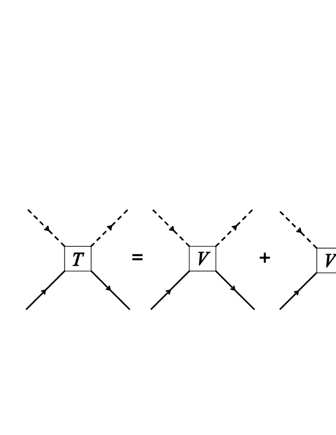
FIG. 1.: Schematic picture of the Bethe Salpeter Equation.

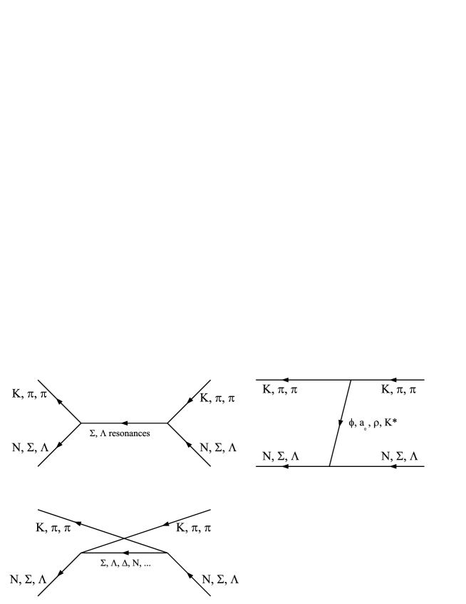
FIG. 2.: Feynman diagrams used in the calculation. In these diagrams the time runs from the right to the left, as usual in matrix elements.

FIG. 3.: Total cross sections

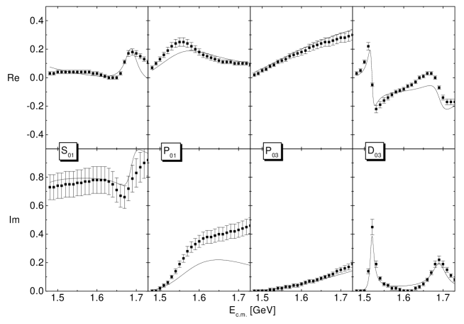
FIG. 4.: PWA [12] and our calculation for $KN\rightarrow KN$, $I=0$.

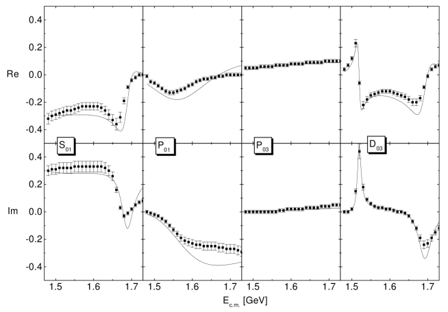
FIG. 5.: PWA [12] and our calculation for $KN\rightarrow\pi\Sigma$, $I=0$.

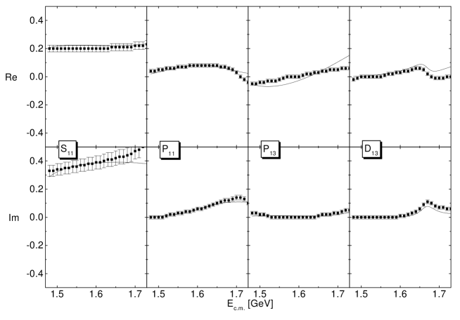
FIG. 6.: PWA [12] and our calculation for $KN\rightarrow KN$, $I=1$.

FIG. 7.: PWA [12] and our calculation for $KN\rightarrow\pi\Sigma$, $I=1$.

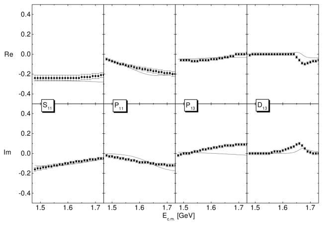
FIG. 8.: PWA [12] and our calculation for $KN\rightarrow\pi\Lambda$, $I=1$.

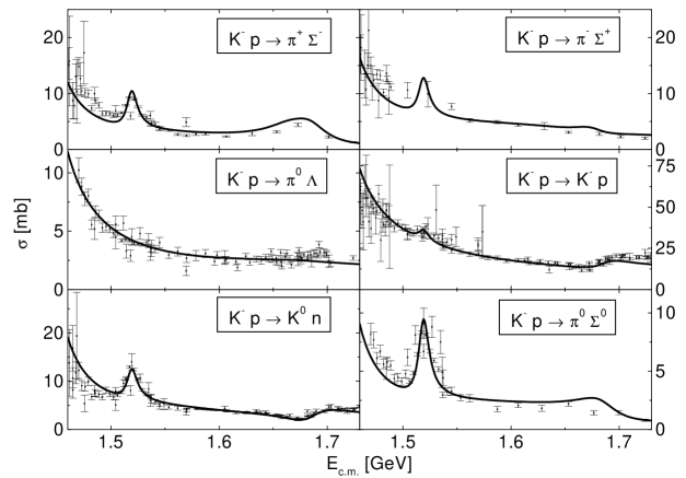
FIG. 9.: Comparison of total cross sections for various reactions with data from [15] used in the fit.

FIG. 10.: The upper three plots show differential cross sections for the reaction $K^{-}p\rightarrow K^{-}p$, the lower ones for the reaction $K^{-}p\rightarrow\overline{K}^{0}n$. The data are taken from the references given in table I.

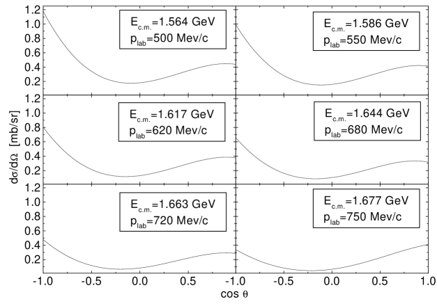
FIG. 11.: Differential cross sections for the reaction $K^{-}p\rightarrow\overline{K}^{0}n$.

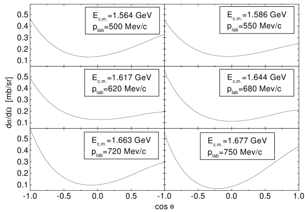
FIG. 12.: Differential cross sections for the reaction $K^{-}p\rightarrow\pi^{0}\Sigma^{0}$.

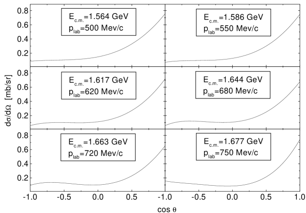
FIG. 13.: Differential cross sections for the reaction $K^{-}p\rightarrow\pi^{0}\Lambda$.

REFERENCES

- [1] The Particle Data Group, The Europ. Phys. Jrn. C3, Vol 1-4 (1998).
- [2] D.M. Manley, R.A. Arndt, Y. Goradia and V.L. Teplitz, Phys. Rev. D30, 904 (1984); D.M. Manley and E.M. Saleski, Phys. Rev. D45, 4002 (1992).
- [3] T. Feuster and U. Mosel, Phys. Rev. C58, 457 (1998); Phys. Rev. C59, 460 (1999).
- [4] C. Bennhold, A. Waluyo, H. Haberzettl, T. Mart, G. Penner, T. Feuster, U. Mosel, L. Tiator, Cambridge 1998, Electronuclear physics with internal targets and the BLAST detector, 225; C. Bennhold, T. Mart, A. Waluyo, H. Haberzettl, G. Penner, T. Feuster, U. Mosel, nucl-th/9901066, Talk given at Workshop on Electron Nucleus Scattering, Marciana Marina, Isola d’Elba, Italy, 22-26 June 1998;
- [5] C. Bennhold, A. Waluyo, H. Haberzettl, T. Mart, G. Penner, U. Mosel nucl-th/0008024.
- [6] H. Haberzettl, C. Bennhold, T. Mart, T. Feuster, Phys. Rev. C58, R40 (1998).
- [7] B.C. Pearce and B.K. Jennings, Nucl. Phys. A528, 655 (1991).
- [8] G. Penner, private communications.
- [9] T. S. Mast et al., Phys. Rev. D14, 13 (1976).
- [10] C. J. Adams et al., Nucl. Phys. B96, 54 (1975).
- [11] M. Alston-Garnjost et al., Phys. Rev. D17, 2226 (1978).
- [12] G. P. Gopal et al., Nucl. Phys. B119, 362 (1977).
- [13] W. Langbein, F. Wagner, Nucl. Phys. B47, 477 (1972).
- [14] M. Alston-Garnjost et al., Phys. Rev. D18, 182 (1978).
- [15] A. Baldini, V. Flaminio, W. G. Moorhead, D. R. O. Morrison, Landolt-Börnstein Band 12a, Springer, Berlin 1988.
- [16] B. Nefkens, private communications.
- [17] Hungchong Kim, Takumi Doi, Makoto Oka and Su Huong Lee, nucl-th/0002011.
- [18] A. J. Buchmann and E. M. Henley, Phys. Lett. B484, 255 (2000).
- [19] G. Morpurgo, Phys. Rev. D40, 2997 (1989); Phys. Rev. D40, 3111 (1989).
- [20] G. Höhler, -Newsletter 9, 1 (1993).