Quark Models of Baryon Masses and Decays

Abstract

Abstract

The application of quark models to the spectra and strong and electromagnetic couplings of baryons is reviewed. This review focuses on calculations which attempt a global description of the masses and decay properties of baryons, although recent developments in applying large $N_{c}$ QCD and lattice QCD to the baryon spectrum are described. After outlining the conventional one-gluon-exchange picture, models which consider extensions to this approach are contrasted with dynamical quark models based on Goldstone-boson exchange and an algebraic collective-excitation approach. The spectra and electromagnetic and strong couplings that result from these models are compared with the quantities extracted from the data and each other, and the impact of various model assumptions on these properties is emphasized. Prospects for the resolution of the important issues raised by these comparisons are discussed.

Contents

toc

I Introduction

The quark model of hadron spectroscopy predated quantum chromodynamics (QCD) by about twenty years and, in a very real sense, led to its development. The puzzle surrounding the ground state decuplet led to a number of postulates, including Greenberg’s ‘parastatistics of order three’ [1], a precursor to the hypothesis of color and, eventually, to the development of QCD. In addition, the early quark model has led to what is sometimes regarded with some contempt, the quark potential model. This model is an attempt to go beyond the global symmetries of the original quark model, which was, in essence, a symmetry-based classification scheme for the proliferating hadrons. The potential model attempted to include dynamics, with the dynamics arising from an inter-quark potential.

Despite the widespread acceptance of QCD as the theory of the strong interaction, there is, as yet, no obviously successful way to go from the QCD Lagrangian to a complete understanding of the multitude of observed hadrons and their properties. Lattice QCD calculations offer a bright promise, but calculations for anything but spectra and static properties like magnetic moments are still a long way off, and even for the spectra of excited states such calculations are just getting under way. Other methods, such as large $N_{c}$ QCD, and effective field theory approaches, also appear to be somewhat limited in their scope, and would seem, by their very nature, to be unable to provide the global yet detailed understanding that is necessary for strong interaction physics. It is in this sense and in this context that the quark potential model is currently an indispensable tool for guiding our understanding. As an illustration, note that the very successful heavy quark effective theory had its origins in a quark model calculation.

In its various forms, the quark potential model has had a large number of successes. The spectra of mesons and baryons, as well as their strong, weak and electromagnetic decays, have all been treated within the framework of this model and the successes of this program can not be dismissed as completely spurious. In addition, the predictions of the model are always to be compared with expectations from QCD, in the continuing effort to understand the intra-hadron dynamics of non-perturbative QCD and confinement.

The study of baryon spectroscopy raises two very important global questions that hint at the interplay between the quark model and QCD. The first of these is the fact that, in many of its forms, the quark model predicts a substantial number of ‘missing’ light baryons which have not so far been observed. There have been two possible solutions postulated for this problem. One solution is that the dynamical degrees of freedom used in the model, namely three valence quarks, are not physically realized. Instead, a baryon consists of a quark and a diquark, and the reduction of the number of internal degrees of freedom leads to a more sparsely populated spectrum. Note, however, that even this spectrum contains more states than observed. A second possible solution is that the missing states couple weakly to the formation channels used to investigate the states, and so give very small contributions to the scattering cross sections. Investigation of other formation channels should lead to the discovery of some of these missing states in this scenario.

The second outstanding question is the fact that, in addition to the usual three quark states, QCD predicts the existence of baryons with ‘excited glue’, the so-called hybrid baryons. Unlike mesons, all half-integral spin and parity quantum numbers are allowed in the baryon sector, so that experiments may not simply search for baryons with exotic quantum numbers in order to identify such hybrid states. Furthermore, no decay channels are a priori forbidden. These two facts make identification of a baryonic hybrid singularly difficult. If new baryon states are discovered at any of the experimental facilities around the world, they can be interpreted either as one of the missing baryons predicted by the quark model, or as one of the undiscovered hybrid states predicted by QCD. Indeed, some authors have suggested that a few of the known baryons could be hybrid states.

These questions about baryon physics are fundamental. If no new baryons are found, both QCD and the quark model will have made incorrect predictions, and it would be necessary to correct the misconceptions that led to these predictions. Current understanding of QCD would have to be modified, and the dynamics within the quark model would have to be changed. If a substantial number of new baryons are found, it would be necessary to determine whether they were three-quark states or hybrids or, as is likely, some admixture. It is only by comparing the experimentally measured properties of these states with model (or lattice QCD) predictions that this determination can be made. As lattice calculations are only now beginning to address the questions of light hadron spectroscopy in a serious fashion, the quark model may be expected to play a vital role for many years to come.

An excellent review article summarizing the situation for baryon physics in the quark model in 1983 was written by Hey and Kelly [2]. This review will, therefore, concentrate on the developments in the field which have taken place since then. It will be necessary, however, to go into some detail about earlier calculations in order to put modern work into perspective. For example, the successes and failures of one-gluon-exchange based models in describing baryon properties need to be understood before examining alternative models. It is also not enough to describe one aspect of baryon physics such as masses, or one type of baryon, since there have existed for some time models which describe with reasonable success the masses and strong and electromagnetic couplings of all baryons. Furthermore, these models are equally useful in a description of meson physics. Within the context of models, insight can only be gained into nonperturbative QCD by comparing predictions to experiment, in as many aspects as possible. Spectra pose only mild tests of models; strong and electromagnetic decays and electromagnetic form factors pose more stringent tests.

By far the most baryon states have been extracted from $\pi$N and $\bar{K}N$ elastic and inelastic scattering data (24 and 22 well established 3 and 4* states [3] with spin assignments, respectively), and so most of the available information on baryon resonances is for nonstrange and strangeness $-1$ baryons. For this reason this article will mainly concentrate on models which make predictions for the static properties and the strong and electromagnetic transitions of all of these states. Such models can also be extended to multiply-strange baryons and heavy-quark baryons, and the best of them are successful in predicting the masses and magnetic moments of the ground states and the masses of the few excited states of these baryons that have been seen. Models which describe the spectrum in the absence of a strong decay model are of limited usefulness. This is because the predicted spectrum must be compared to the results of an experiment which examines excited baryons using a specific formation and decay channel. If a model predicts a baryon state which actually couples weakly to either or both of these channels, this state cannot be identified with a resonant state from analyses of that experiment.

Considerations of space do not allow a proper treatment here of the electromagnetic transition form factors of excited nonstrange baryons, or of the magnetic moments or other electromagnetic properties of the nucleon and other ground states, even though intense theoretical and experimental effort has been brought to bear on these issues. In particular, it has been shown in a substantial literature that the static properties of ground state baryons such as magnetic moments, axial-vector couplings, and charge radii, are subject to large corrections from relativistic effects and meson-loop couplings. This is also true of the transition form factors. In order to avoid a necessarily superficial treatment, the description of these quantities in the various models of the spectrum dealt with here is not discussed.

II Ground state baryon masses

A mass formulae based on symmetry

The interactions of quarks in baryons depend weakly on the masses of the quarks involved in the interaction, and depend very weakly on their electric charges. The small size of the strange-light quark mass difference compared to the confinement scale means that the properties of baryon states which differ only by the interchange of light and strange quarks are quite similar. The much smaller difference between the masses of the up and down quarks means that the properties of baryon states which differ only by the interchange of up and down quarks are very similar. The further observation that the properties of such states should be independent of an arbitrary continuous rotation of each quark’s flavor in the $(u,d,s)$ flavor space led to the notion of the approximate SU(3)_f symmetry and the much better isospin symmetry which is found in the spectrum of the ground-state baryons. Although this continuous symmetry exists, of course physical states are discrete with an integer number of quarks of each flavor.

The most important explicit SU(3)_f-symmetry breaking effect is the strange-light quark mass difference; isospin-symmetry breaking is small by comparison, and has roughly equally important contributions from the up-down quark mass difference and from electromagnetic interactions between the quarks. The charge averaged masses of the octet of $J^{P}={\textstyle{1\over 2}}^{+}$ ground state baryon masses should, therefore, be related by the addition of $m_{s}-m_{u,d}$ for each light quark replaced by a strange quark. This assumes that each state has the same kinetic and potential energy, which is only approximately true due to the dependence of their expectation values on the quark masses. This observation leads to mass relations between baryons which differ only by the addition of a strange quark, for example the Gell-Mann–Okubo mass formula, which eliminates the parameters $M_{0}$, $m_{u,d}$ and $m_{s}$ from the assumed masses

$$M_{N} = M_{0}+3m_{u,d}$$ (1)

$$M_{\Lambda}=M_{\Sigma} = M_{0}+2m_{u,d}+m_{s}$$ (2)

$$M_{\Xi} = M_{0}+m_{u,d}+2m_{s}$$ (3)

of the $J^{P}={\textstyle{1\over 2}}^{+}$ baryons to find

$${M_{\Sigma}+3M_{\Lambda}\over 2}=M_{N}+M_{\Xi}.$$ (4)

With this simple argument any linear combination of $M_{\Sigma}$ and $M_{\Lambda}$ should work; however, the particular linear combination chosen here makes this relation good to about 1%. This is based on the assumption of a baryon mass term in an effective Lagrangian of the form $\bar{\psi}(a+b\lambda_{8})\psi$, where $\psi$ is a baryon field which represents SU(3)_f and $\lambda_{8}$ is a Gell-Mann matrix. This form contains only the SU(3)_f singlet and a symmetry-breaking octet term. Using this assumption, called the octet dominance rule, and the calculation [4] of some SU(3)_f recoupling constants for $8\otimes 8=1\oplus 8^{\prime}\oplus 8^{\prime\prime}$, one obtains

$$M_{N} = M_{1}-2M_{8^{\prime}}+M_{8^{\prime\prime}}$$ (5)

$$M_{\Lambda} = M_{1}-M_{8^{\prime}}-M_{8^{\prime\prime}}$$ (6)

$$M_{\Sigma} = M_{1}+M_{8^{\prime}}+M_{8^{\prime\prime}}$$ (7)

$$M_{\Xi} = M_{1}+M_{8^{\prime}}-2M_{8^{\prime\prime}}$$ (8)

which yields the desired relation.

An analysis of $J^{P}={\textstyle{3\over 2}}^{+}$ ground-state decuplet baryon masses taking into account only the quark mass differences yields Gell-Mann’s equal spacing rule

$$M_{\Sigma^{*}}-M_{\Delta}=M_{\Xi^{*}}-M_{\Sigma^{*}}=M_{\Omega}-M_{\Xi^{*}},$$ (9)

which compare well to the charge-averaged experimental mass splittings of 153, 149 and 139 MeV respectively. The systematic deviations can be attributed to a quark-mass-dependent hyperfine interaction which splits these states from their $J^{P}={\textstyle{1\over 2}}^{+}$ partners. This topic will be revisited below.

Okubo [5] and Gürsey and Radicati [6] derive a mass formula for the ground-state baryons using matrix elements of a mass operator with $J^{P}=0^{+}$, isospin, hypercharge ($Y=2[Q-I_{3}]$), and strangeness zero, and with the assumptions that it contains only one and two-body operators and octet dominance they find

$$M=a+bY+c\left[I(I+1)-Y^{2}/4\right]+dJ(J+1),$$ (10)

which contains the above relations for the $J^{P}={\textstyle{1\over 2}}^{+}$ octet and ${\textstyle{3\over 2}}^{+}$ decuplet. Equation (10) also contains the SU(6) relation [7]

$$M_{\Sigma^{*}}-M_{\Sigma}=M_{\Xi^{*}}-M_{\Xi}$$ (11)

which takes into account energy differences due to the spin of the states and their flavor structure. This compares well to the experimental differences of 192 and 215 MeV, respectively. The deviation from this rule can be explained by a quark-mass dependent hyperfine interaction and wave function size.

An example of a mass relation which takes into account both the approximate SU(3)_f and isospin symmetries of the strong interaction is the Coleman-Glashow relation, which can be expressed as a linear combination of $I=1$ mass splittings which should be zero [8],

$$N_{1}+\Xi_{1}-\Sigma_{1}=0,$$ (12)

where

$$N_{1} = M_{p}-M_{n}$$ (13)

$$\Sigma_{1} = M_{\Sigma^{+}}-M_{\Sigma^{-}}$$ (14)

$$\Xi_{1} = M_{\Xi^{0}}-M_{\Xi^{-}}.$$ (15)

This relation holds to within experimental errors on the determination of the masses. Jenkins and Lebed [8] analyze this and many other ground-state baryon octet and decuplet isospin splittings in a $1/N_{c}$ expansion which is combined with perturbative flavor breaking. They find that this relation should receive corrections at the level of $\epsilon\epsilon^{\prime}/N_{c}^{2}$, where $\epsilon$ is a small SU(3)_f symmetry breaking, and where $\epsilon^{\prime}$ is a much smaller isospin-symmetry breaking parameter. This pattern of symmetry breaking is what is observed experimentally. This relation is found to be preserved by the explicitly isospin and flavor-symmetry breaking interactions in a dynamical potential model to be described later [9]. Jenkins and Lebed’s work establishes clear evidence for a $1/N_{c}$ hierarchy of the observed mass splittings, which differs from that based on SU(6) symmetry.

B QCD-based dynamical models

Mass-formula approaches based solely on symmetry are not able to explain the sign of the $\Delta-N$ and $\Sigma-\Lambda$ splittings; this requires a dynamical model. Development of QCD led to models of these splittings based on one-gluon exchange, such as the nonrelativistic potential model of De Rujula, Georgi, and Glashow (DGG) [10] and the MIT bag model of Refs. [11, 12]. The DGG model uses unperturbed eigenstates which are SU(6) multiplets with unknown masses, and then mass formulae are derived using the Fermi-Breit interaction between colored quarks from one-gluon exchange. For ground states the important interaction is the Fermi contact term, which leads to ground-state baryon masses

$$M=\sum_{i=1}^{3}m_{i}+{2\alpha_{s}\over 3}{8\pi\over 3}\langle\delta^{3}({\bf r})\rangle\sum_{i<j=1}^{3}{{\bf S}_{i}\cdot{\bf S}_{j}\over m_{i}m_{j}},$$ (16)

where the $m_{i}$ are the “constituent” quark effective masses and where, by exchange symmetry of the ground state spatial wave functions, $\langle\delta^{3}({\bf r}_{ij})\rangle$ is the same for any one of the relative coordinates ${\bf r}_{ij}={\bf r}_{i}-{\bf r}_{j}$. In the limit of SU(3)_f symmetry this expectation value will also be the same for all ground-state baryons and so the coefficient of the spin sum will be a constant. Taking this coefficient and the constituent quark masses $m_{u}=m_{d}\not=m_{s}$ as three parameters, a three parameter formula for the ground state masses is obtained. Equations (4) and (11) follow to first order in $(m_{s}-m_{u,d})/m_{u,d}$, and the interaction naturally explains the sign of the decuplet-octet mass difference, since the decuplet states have all three quark spins aligned and so have higher energy with this interaction. The size of the splitting is related to the QCD coupling constant $\alpha_{s}$, albeit at low values of $Q^{2}$ where it need not be small.

The mass dependence of the spin-spin interaction above leads to the relation

$${M_{\Sigma}-M_{\Lambda}\over M_{\Delta}-M_{N}}={2\over 3}\left(1-{m_{u,d}\over m_{s}}\right)$$ (17)

between the $\Sigma-\Lambda$ and $\Delta-N$ mass splittings. With the rough values of the effective quark masses $m_{s}\simeq 550$ MeV and $m_{u,d}\simeq$ 330 MeV implied by a naive additive nonrelativistic quark model fit to the size of the ground-state octet magnetic moments, an apparently very good explanation of the relative size of these two splittings is obtained. This is, however, subject to substantial corrections. Distortions of the wave functions due to the heavier strange quark mass increase the size of the contact interactions between the strange quark and the light quarks, which tends to compensate for the lowered size of the interaction due to the mass factor in Eq. (16), lowering the $\Sigma-\Lambda$ splitting [13, 14] by about 30 MeV. Equation (17) also holds only in first-order (wave function) perturbation theory, and in the calculation of Ref. [14] second-order effects due to a stronger mixing with N=2 levels in the $\Sigma$ than the $\Lambda$ open up the splitting again by about the same amount, so that this relation happens to survive these corrections.

The bag model calculation of DeGrand, Jaffe, Johnson, and Kiskis [15, 16] is relativistic, and confines the quarks to the interior of hadrons by a bag pressure term with a parameter $B$ used to set the scale of the baryon masses. The consequence of this confinement is that the equations of motion inside the bag are supplemented by a homogeneous boundary condition which eliminates quark currents across the bag surface, and a quadratic boundary condition that balances the pressure from the quarks and gluons with that of the bag locally on the surface. The quarks interact among themselves relatively weakly by gluon exchange which is treated in lowest order, and which gives a short-distance interaction between the quarks of the same kind as that of DGG. The strange quark mass is larger than the light-quark mass, to which the spectrum is rather insensitive and which can be taken to be zero. As a consequence, there is flavor dependence to the short-distance interaction which explains the sign of the $\Sigma-\Lambda$ splitting, although the calculated size is about half of the observed value. Assuming that the bag radius parameter $R$ is the same for each state also leads to the Gell-Mann-Okubo and equal spacing relations in Eq. (4) and Eq. (11). The model has four parameters, which are $B$, the quark-gluon coupling constant $\alpha_{c}$, the strange quark mass, and a parameter $Z_{0}$ associated with the zero-point energy for quantum modes in the bag. The cavity radius $R$ is fixed by the quadratic boundary condition for each hadron considered. A reasonable fit to ground state masses and static properties is attained.

The authors of Refs. [15, 16] point out that in their model the momentum of a 300 MeV constituent quark is large, of the order of 500 MeV, and conclude that the nonrelativistic models which do not properly take into account the quark kinetic energy are inconsistent. They also point out that the quarks are confined by a dynamical mechanism which must carry energy (in their case it is the bag energy), and that a prescription for reconciling the confining potential locally with relativity is necessary. On the other hand, it is difficult to ensure that the center of mass of a hadron state is not moving when the dynamics of each of the constituents is the solution of a one-body Dirac equation. Such spurious states are therefore mixed in with the states of interest and will affect their masses and properties. Nonrelativistic models have no such difficulty. Some of these points will be revisited below.

Other models of ground state baryons include the cloudy bag model of Théberge, Thomas and Miller [17], which incorporates chiral invariance by allowing a cloud of pion fields to couple to the confined quarks only at the surface of the MIT bag, and is used to describe the pion-nucleon scattering cross section in the $P_{33}$ partial wave in the region of the $\Delta$ resonance. The result is that both pion-nucleon scattering (Chew-Low) diagrams and an elementary $\Delta$ diagram contribute, with about 20% and 80% contributions to the $\pi N$ resonance strength, respectively.

Ground-state baryon masses have also been examined in the chiral perturbation theory [18] and in large $N_{c}$ QCD [19] by Jenkins. The former work shows that the Gell-Mann-Okubo relation Eq. (4) and Gell-Mann’s equal spacing rule Eq. (9) are consistent with chiral perturbation theory up to incalculable corrections of order the strange quark current mass squared, or of order 20 MeV. Both relations hold to better than this accuracy experimentally. The latter work shows that baryon hyperfine mass splittings, which were known from previous work to first appear at order $1/N_{c}$, are identical to those produced by the operator ${\bf J}^{2}$, which is consistent with the Gursey-Radicati formula Eq. (10) and with the Skyrme model[20]. The masses of the nucleon, $\Delta$, and the lowest-lying $D_{13}$ $(J^{P}=3/2^{-})$ $N^{*}$ resonance are also calculated with QCD sum rules by Belyaev and Ioffe [21], which leads to a 10-15% overestimate with the parameters used there.

Recent progress in lattice calculations with improved quark and gluon actions and inevitable improvements in computer speed have led to results for $N$, $\Delta$, and vector meson masses for full (unquenched) QCD with two dynamical quark flavors [22, 23]. The results are mainly in a dynamical regime where the pion mass is above 500 MeV, with one recent calculation on a larger lattice at a lower (300-400 MeV) pion mass. These results therefore require extrapolation to the physical pion mass, which Leinweber, Thomas, Tsushima, and Wright [24] show is complicated by non-linearity in the pion mass squared due to the $N\pi$ threshold, and by non-analytic behavior associated with dynamical chiral symmetry breaking. They examine the corrections to the extrapolated light baryon masses from the pion-induced self-energies implied by chiral perturbation theory. They defer making conclusions about the agreement between extrapolated lattice results and experiment until systematic errors in the full QCD calculations are reduced from the current 10% level and lattice measurements are made at lower pion masses.

As an example of quenched lattice results, where the reaction of dynamical sea quarks is turned off, the CP-PACS collaboration [23] spectrum is shown in Figure 1. Although the quenched results show systematic deviations from the experimental masses, the spectrum shows a good pattern of SU(3)_f breaking mass splittings, and if the strange-quark mass is fixed by fitting to the $\phi$ rather than the kaon mass, baryon masses are fit to an error of at most -6.6% (the nucleon mass).

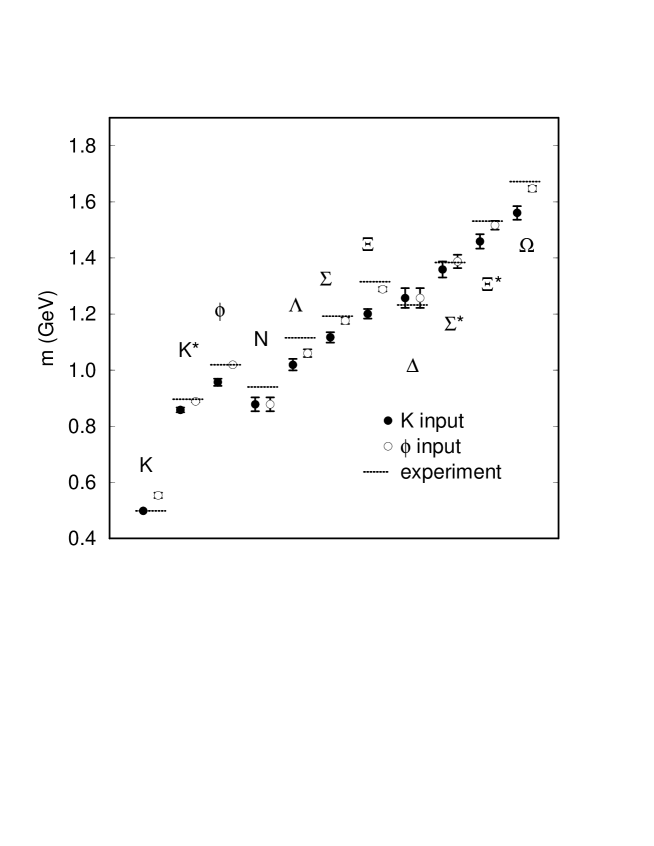
FIG. 1.: Results of CP-PACS simulation of the flavor non-singlet light hadron spectrum in quenched lattice QCD with Wilson quark action.

Lattice QCD calculations should eventually be able to describe the properties of the lowest-lying baryon states of any flavor of baryon with small angular momentum, such as the P-wave baryons. However, for technical reasons it may remain difficult to extract signals for the masses of excited states beyond the second recurrence of a particular set of flavor, spin, and parity quantum numbers, and for high angular momentum states. It is, therefore, likely that models of the kind described below will remain useful for the description of excited baryons.

III Excited baryon masses in the nonrelativistic model

A negative-parity excited baryons in the Isgur-Karl model

Many studies of excited baryon states were made based on the observations of De Rujula, Georgi, and Glashow [10]; the most detailed and phenomenologically successful of these is the model of Isgur and Karl and their collaborators [25, 26, 27, 28, 29, 30, 14, 31, 32, 33]. This and other potential models have implicit assumptions which should be made clear here. If one probes the proton with an electron which transfers an amount of energy and momentum modest compared to the confinement scale, then it may be useful to describe the proton in this ‘soft’ region as being made up of three constituent quarks. In such models the light ($u$ and $d$) constituent (effective) quarks have masses of roughly 200 to 350 MeV, and can be thought of as extended objects, i.e. ‘dressed’ valence quarks. Strange quarks are about 150-200 MeV heavier. These are not the partons required to describe deep inelastic scattering from the proton; their interactions are described in an effective model which is not QCD but which is motivated by it.

It is also assumed that the gluon fields affect the quark dynamics by providing a confining potential in which the quarks move, which is effectively pair-wise linear at large separation of the quarks, and at short distance one-gluon exchange provides a Coulomb potential and the important spin-dependent potential. Otherwise the effects of the gluon dynamics on the quark motion are neglected. This model will obviously have a limited applicability: to ‘soft’ (low-$Q^{2}$ or coarse-grid) aspects of hadron structure, and to low-mass hadrons where gluonic excitation is unlikely. Similarly, since only three quarks components have been allowed in a baryon [other Fock-space components like $qqq(q\bar{q})$ have been neglected], it will strictly only be applicable to hadrons where large mass shifts from couplings to decay channels are not expected. Recent progress in understanding these mass shifts, and the effects of including the dynamics of the glue, will be described below.

Isgur and Karl solve the Schrödinger equation $H\Psi=E\Psi$ for the three valence-quark system baryon energies and wave functions, with a Hamiltonian

$$H=\sum_{i}\left(m_{i}+{{\bf p}_{i}^{2}\over 2m_{i}}\right)+\sum_{i<j}\left(V^{ij}+H^{ij}_{\rm hyp}\right),$$ (18)

where the spin-independent potential $V^{ij}$ has the form $V^{ij}=C_{qqq}+br_{ij}-2\alpha_{s}/3r_{ij}$, with $r_{ij}=|{\bf r}_{i}-{\bf r}_{j}|$. In practice, $V^{ij}$ is written as a harmonic-oscillator potential $Kr_{ij}^{2}/2$ plus an unspecified anharmonicity $U_{ij}$, which is treated as a perturbation. The hyperfine interaction $H^{ij}_{\rm hyp}$ is the sum

$$H^{ij}_{\rm hyp}={2\alpha_{s}\over 3m_{i}m_{j}}\left\{{8\pi\over 3}{\bf S}_{i}\cdot{\bf S}_{j}\delta^{3}({\bf r}_{ij})+{1\over r_{ij}^{3}}\left[{3({\bf S}_{i}\cdot{\bf r}_{ij})({\bf S}_{j}\cdot{\bf r}_{ij})\over r_{ij}^{2}}-{\bf S}_{i}\cdot{\bf S}_{j}\right]\right\}$$ (19)

of contact and tensor terms arising from the color magnetic dipole-magnetic dipole interaction. In this model the spin-orbit forces which arise from one-gluon exchange and from Thomas precession of the quark spins in the confining potential are deliberately neglected; their inclusion spoils the agreement with the spectrum, since the resulting splittings tend to be too large. The relative strengths of the contact and tensor terms are as determined from the Breit-Fermi limit [the expansion to O$(p^{2}/m^{2})$] of the one-gluon exchange potential. Note that there are also spin-independent, momentum-dependent terms in the expansion to this order, such as Darwin and orbit-orbit interaction terms, which are neglected by Isgur and Karl.

Baryon states are written as the product of a color wave function $C_{A}$ which is totally antisymmetric under the exchange group $S_{3}$, and a sum $\sum\psi\chi\phi$, where $\psi$, $\chi$, and $\phi$ are the spatial, spin, and flavor wave functions of the quarks respectively. The spatial wave functions are chosen to represent $S_{3}$ in the case of baryons with equal-mass quarks, and the spin wave functions automatically do so. The sum is constructed so that it is symmetric under exchange of equal mass quarks, and also implicitly includes Clebsch-Gordan coefficients for coupling the quark orbital angular momentum ${\bf L}$ with the total quark spin ${\bf S}$.

$S_{3}$ has three irreducible representations. The two one-dimensional representations are the antisymmetric (denoted $A$), and symmetric ($S$) representations. The two-dimensional mixed-symmetry ($M$) representation has states $M^{\rho}$ and $M^{\lambda}$ which transform among themselves under exchange transformations. For example, $(12)M^{\rho}=-M^{\rho}$, $(12)M^{\lambda}=M^{\lambda}$, and $(13)M^{\rho}=M^{\rho}/2-\sqrt{3}M^{\lambda}/2$, $(13)M^{\lambda}=-\sqrt{3}M^{\rho}/2-M^{\lambda}/2$. The spin wave functions $\chi$ found from coupling three spins-${\textstyle{1\over 2}}$ are an example of such a representation,

$${\textstyle{1\over 2}}\otimes{\textstyle{1\over 2}}\otimes{\textstyle{1\over 2}}=(1\oplus 0)\otimes{\textstyle{1\over 2}}=({\textstyle{3\over 2}}\oplus[{\textstyle{1\over 2}}]_{\rho})\oplus[{\textstyle{1\over 2}}]_{\lambda}.$$ (20)

The spin-${\textstyle{3\over 2}}$ wave function $\chi^{S}$ is totally symmetric, and the two spin-${\textstyle{1\over 2}}$ wave functions $\chi^{M_{\lambda}}$ (from $1\otimes{\textstyle{1\over 2}}$) and $\chi^{M_{\rho}}$ (from $0\otimes{\textstyle{1\over 2}}$) form a mixed-symmetry pair,

$$\chi^{S}_{{\textstyle{3\over 2}},{\textstyle{3\over 2}}} = |\uparrow\uparrow\uparrow\,>,\ \ \chi^{\rho}_{{\textstyle{1\over 2}},{\textstyle{1\over 2}}}={1\over\sqrt{2}}\left\{|\uparrow\downarrow\uparrow\,>-|\downarrow\uparrow\uparrow\,>\right\},$$ (21)

$$\chi^{\lambda}_{{\textstyle{1\over 2}},{\textstyle{1\over 2}}} = -{1\over\sqrt{6}}\left\{|\downarrow\uparrow\uparrow\,>+|\uparrow\downarrow\uparrow\,>-2|\uparrow\uparrow\downarrow\,>\right\},$$ (22)

where the subscripts are the total spin and its projection, and other projections can be found by applying a lowering operator.

The construction of the flavor wave functions $\phi$ for nonstrange states proceeds exactly analogously to that of the spin wave functions, using isospin. They either have mixed symmetry ($N,I={\textstyle{1\over 2}}$) or are totally symmetric ($\Delta,I={\textstyle{3\over 2}}$),

$$\phi^{S}_{\Delta^{++}} = uuu,\ \ \phi^{S}_{\Delta^{+}}={1\over\sqrt{3}}\left\{uud+udu+duu\right\},\ {\rm etc.},$$ (23)

$$\phi^{M_{\rho}}_{p} = {1\over\sqrt{2}}\left\{udu-duu\right\},\ \ \phi^{M_{\rho}}_{n}={1\over\sqrt{2}}\left\{udd-dud\right\},$$ (24)

$$\phi^{M_{\lambda}}_{p} = -{1\over\sqrt{6}}\left\{duu+udu-2\,uud\right\},\ \ \phi^{M_{\lambda}}_{n}={1\over\sqrt{6}}\left\{udd+dud-2\,ddu\right\}.$$ (25)

For strange (and heavy-quark) baryons it is advantageous to use a basis which makes explicit SU(3)_f breaking and so does not antisymmetrize under exchange of the unequal mass quarks. Since the mass differences $m_{s}-(m_{u}+m_{d})/2$ (and $m_{c}-[m_{u}+m_{d}]/2$, etc.) are substantial on the scale of the average quark momentum, there are substantial SU(3)_f breaking differences between, for example, the spatial wave functions of the ground state of the nucleon and that of the ground state $\Lambda$. For such states the ‘$uds$ basis’ is used, which imposes symmetry only under exchange of equal mass quarks, and adopt the flavor wave functions

$$\phi_{\Lambda} = {1\over\sqrt{2}}(ud-du)s,$$ (26)

$$\phi_{\Sigma^{+,0,-}} = uus,{1\over\sqrt{2}}(ud+du)s,dds,$$ (27)

$$\phi_{\Xi^{0,-}} = ssu,ssd,$$ (28)

$$\phi_{\Omega^{-}} = sss.$$ (29)

Note that these flavor wave functions are all either even or odd under (12) exchange, as are the spin wave functions in Eq. (22). This allows sums $\sum\psi\chi\phi$ to be easily built for these states which are symmetric under exchange of the equal mass quarks, taken as quarks 1 and 2.

In zeroth order in the anharmonic perturbation $U$ and hyperfine perturbation $H_{\rm hyp}$, the spatial wave functions $\psi$ are the harmonic-oscillator eigenfunctions $\psi_{NLM}(\mbox{\boldmath$\rho$},\mbox{\boldmath$\lambda$})$, where

$$\mbox{\boldmath$\rho$}=({\bf r}_{1}-{\bf r}_{2})/\sqrt{2},\ \ \mbox{\boldmath$\lambda$}={1\over\sqrt{6}}({\bf r}_{1}+{\bf r}_{2}-2{\bf r}_{3})$$ (30)

are the Jacobi coordinates which separate the Hamiltonian in Eq. (18) into two independent three-dimensional oscillators when $U=H_{\rm hyp}=0$. The $\psi_{NLM}(\mbox{\boldmath$\rho$},\mbox{\boldmath$\lambda$})$ can then be conveniently written as sums of products of three-dimensional harmonic oscillator eigenstates with quantum numbers $(n,l,m)$, where $n$ is the number of radial nodes and $|l,m\rangle$ is the orbital angular momentum, and where the zeroth order energies are $E=(N+{\textstyle{3\over 2}})\omega=(2n+l+{\textstyle{3\over 2}})\omega$, with $\omega^{2}=3K/m$.

For nonstrange states these sums are arranged so that the resulting $\psi_{NLM}$ have their orbital angular momenta coupled to ${\bf L}=\mbox{\boldmath$l_{\rho}$}+\mbox{\boldmath$l_{\lambda}$}$, and so that the result represents the permutation group $S_{3}$. The resulting combined six-dimensional oscillator state has energy $E=(N+3)\omega$, where $N=2(n_{\rho}+n_{\lambda})+l_{\rho}+l_{\lambda}$, and parity $P=(-1)^{l_{\rho}+l_{\lambda}}$.

Ground states are described, in zeroth order in the perturbations, by basis states with $N=0$. For example the nucleon and $\Delta$ ground states have, in zeroth order, the common spatial wave function

$$\psi^{S}_{00}={\alpha^{3}\over\pi^{\textstyle{3\over 2}}}e^{-\alpha^{2}(\rho^{2}+\lambda^{2})/2},$$ (31)

where the notation is $\psi^{\pi}_{LM}$ with $\pi$ labeling the exchange symmetry, and the harmonic oscillator scale constant is $\alpha=(3Km_{u})^{1\over 4}$. For $\Lambda$ and $\Sigma$ states the generalization is to allow the wave function to have an asymmetry between the $\rho$ and $\lambda$ oscillators

$$\psi_{00}={\alpha_{\rho}^{\textstyle{3\over 2}}\alpha_{\lambda}^{\textstyle{3\over 2}}\over\pi^{\textstyle{3\over 2}}}e^{-({\alpha_{\rho}^{2}}\rho^{2}+{\alpha_{\lambda}^{2}}\lambda^{2})/2},$$ (32)

where $\alpha_{\rho}=(3Km)^{1\over 4}$, with $m=m_{1}=m_{2}=(m_{u}+m_{d})/2$, and $\alpha_{\lambda}=(3Km_{\lambda})^{1\over 4}$, with $m_{\lambda}=3mm_{3}/(2m+m_{3})>m$. Note that the orbital degeneracy is now broken, since $\omega_{\rho}^{2}=3K/m>\omega_{\lambda}^{2}=3K/m_{\lambda}$.

In zeroth order, the low-lying negative-parity excited $P$-wave resonances have $N=1$ spatial wave functions with either $l_{\rho}=1$ or $l_{\lambda}=1$. The wave functions used for strange baryons are

$$\psi^{\rho}_{1\pm 1} = \mp{\alpha_{\rho}^{\textstyle{5\over 2}}\alpha_{\lambda}^{\textstyle{3\over 2}}\over\pi^{\textstyle{3\over 2}}}\rho_{\pm}e^{-({\alpha_{\rho}^{2}}\rho^{2}+{\alpha_{\lambda}^{2}}\lambda^{2})/2},$$ (33)

$$\psi^{\lambda}_{1\pm 1} = \mp{\alpha_{\rho}^{\textstyle{3\over 2}}\alpha_{\lambda}^{\textstyle{5\over 2}}\over\pi^{\textstyle{3\over 2}}}\lambda_{\pm}e^{-({\alpha_{\rho}^{2}}\rho^{2}+{\alpha_{\lambda}^{2}}\lambda^{2})/2},$$ (34)

$$\psi^{\rho}_{10} = {\alpha_{\rho}^{\textstyle{5\over 2}}\alpha_{\lambda}^{\textstyle{3\over 2}}\over\pi^{\textstyle{3\over 2}}}\sqrt{2}\rho_{0}e^{-({\alpha_{\rho}^{2}}\rho^{2}+{\alpha_{\lambda}^{2}}\lambda^{2})/2},$$ (35)

and similarly for $\psi^{\lambda}_{10}$, where $\rho_{\pm}\equiv\rho_{x}\pm i\rho_{y}$, $\rho_{0}\equiv\rho_{z}$, etc. For the equal mass case the mixed symmetry states $\psi^{M_{\rho}}$ and $\psi^{M_{\lambda}}$ found from Eq. (35) by equating $\alpha_{\rho}$ and $\alpha_{\lambda}$ are used.

Using the following rules for combining a pair of mixed-symmetry representations,

$${1\over\sqrt{2}}(M^{\rho}M^{\rho}+M^{\lambda}M^{\lambda}) = S,$$ (36)

$${1\over\sqrt{2}}(M^{\rho}M^{\lambda}-M^{\lambda}M^{\rho}) = A,$$ (37)

$${1\over\sqrt{2}}(M^{\rho}M^{\lambda}+M^{\lambda}M^{\rho}) = M^{\rho},$$ (38)

$${1\over\sqrt{2}}(M^{\rho}M^{\rho}-M^{\lambda}M^{\lambda}) = M^{\lambda},$$ (39)

the two nonstrange ground states are, in zeroth order in the perturbations, represented by

$$|N^{2}S_{S}{\textstyle{1\over 2}}^{+}\rangle = C_{A}\psi^{S}_{00}{1\over\sqrt{2}}(\phi^{\rho}_{N}\chi^{\rho}_{\textstyle{1\over 2}}+\phi^{\lambda}_{N}\chi^{\lambda}_{\textstyle{1\over 2}}),$$ (40)

$$|\Delta^{4}S_{S}{\textstyle{3\over 2}}^{+}\rangle = C_{A}\phi^{S}_{\Delta}\psi^{S}_{00}\chi^{S}_{\textstyle{3\over 2}}.$$ (41)

The states are labeled by $|X^{2S+1}L_{\pi}J^{P}\rangle$, where $X=N$ or $\Delta$, $S$ is the total quark spin, $L=S,P,D...$ is the total orbital angular momentum, $\pi=S,M$ or $A$ is the permutational symmetry (symmetric, mixed symmetry, or antisymmetric respectively) of the spatial wave function, and $J^{P}$ is the state’s total angular momentum and parity. Here and in what follows the spin projections $M_{S}$ and Clebsch-Gordan coefficients for the ${\bf J}={\bf L}+{\bf S}$ coupling are suppressed. Another popular notation for classification of baryon states is that of SU(6), which would be an exact symmetry of the interquark Hamiltonian if it was invariant under SU(3)_f, and independent of the spin of the quarks (so that, for example, the ground state octet and decuplet baryons would be degenerate). In this notation there is an SU(3)_f octet of ground state baryons with $(J=)S={\textstyle{1\over 2}}$, giving $(2S+1)\cdot 8=16$ states, plus an SU(3)_f decuplet of ground state baryons with $(J=)S={\textstyle{3\over 2}}$, giving $(2S+1)\cdot 10=40$ states, for 56 states in total. These ground states all have $L^{P}=0^{+}$, so the SU(6) multiplet to which they belong is labelled $[56,0^{+}]$.

The negative-parity $P$-wave excited states occur at $N=1$ in the harmonic oscillator, and have the compositions

$$| N^{4}P_{M}({\textstyle{1\over 2}}^{-},{\textstyle{3\over 2}}^{-},{\textstyle{5\over 2}}^{-})\rangle=C_{A}\chi^{S}_{\textstyle{3\over 2}}{1\over\sqrt{2}}(\phi^{\rho}_{N}\psi^{M_{\rho}}_{1M}+\phi^{\lambda}_{N}\psi^{M_{\lambda}}_{1M}),$$ (42)

$$| N^{2}P_{M}({\textstyle{1\over 2}}^{-},{\textstyle{3\over 2}}^{-})\rangle=C_{A}{1\over 2}\left\{\phi^{\rho}_{N}[\psi^{M_{\rho}}_{1M}\chi^{\lambda}_{\textstyle{1\over 2}}+\psi^{M_{\lambda}}_{1M}\chi^{\rho}_{\textstyle{1\over 2}}]+\phi^{\lambda}_{N}[\psi^{M_{\rho}}_{1M}\chi^{\rho}_{\textstyle{1\over 2}}-\psi^{M_{\lambda}}_{1M}\chi^{\lambda}_{\textstyle{1\over 2}}]\right\},$$ (43)

$$| \Delta^{2}P_{M}({\textstyle{1\over 2}}^{-},{\textstyle{3\over 2}}^{-})\rangle=C_{A}\phi^{S}_{\Delta}{1\over\sqrt{2}}(\psi^{M_{\rho}}_{1M}\chi^{\rho}_{\textstyle{1\over 2}}+\psi^{M_{\lambda}}_{1M}\chi^{\lambda}_{\textstyle{3\over 2}}).$$ (44)

where the notation $({\textstyle{1\over 2}}^{-},{\textstyle{3\over 2}}^{-},{\textstyle{5\over 2}}^{-})$ lists all of the possible $J^{P}$ values from the ${\bf L}+{\bf S}$ coupling. These are members of the $[70,1^{-}]$ SU(6) multiplet, where the 70 is made up of two octets of $S={\textstyle{3\over 2}}$ and $S={\textstyle{1\over 2}}$ states and a decuplet of $S={\textstyle{1\over 2}}$ states as above, plus a singlet $\Lambda$ state[34] with $S={\textstyle{1\over 2}}$.

Isgur and Karl use five parameters to describe the nonstrange and strangeness $S=-1$ P-wave baryons: the unperturbed level of the nonstrange states, about 1610 MeV; the quark mass difference $\Delta m=m_{s}-m_{u}=280$ MeV; the ratio $x=m_{u}/m_{s}=0.6$; the nonstrange harmonic oscillator level spacing $\omega\simeq 520$ MeV; and the strength of the hyperfine interaction, determined by fitting to the $\Delta-N$ splitting which is

$$\delta={4\alpha_{s}\alpha^{3}\over 3\sqrt{2\pi}m_{u}^{2}}\simeq 300\ {\rm MeV},$$ (45)

where $\alpha$, given by $\alpha^{2}=m_{u}\omega=\sqrt{3Km_{u}}$, is the harmonic-oscillator constant used in the nonstrange wave functions. In the strange states two constants $\alpha_{\rho}=\alpha$ and $\alpha_{\lambda}$ are used; their ratio is determined by the quark masses and by separation of the center of mass motion in the harmonic oscillator problem. Note that the effective value of $\alpha_{s}$ implied by these equations is $\alpha_{s}\simeq 0.95$. The value of $\Delta m$ used here is larger than that implied by a simple SU(3)_f analysis of the ground state baryon masses where distortions to the wave functions due to the heavier strange quark are ignored. Taking these effects into account increases the size of $\Delta m$ required to fit the ground states to 220 MeV [14].

FIG. 2.: The hyperfine contact perturbation applied to the P-wave nonstrange baryons.

The result of evaluating the contact perturbation in the nonstrange baryons is the pattern of splittings shown in Figure 2. The tensor part of the hyperfine interaction has generally smaller expectation values, and so is not as important to the spectroscopy as the contact interaction. Isgur and Karl argue, however, that it does cause significant mixing in some states which are otherwise unmixed; this has important consequences for the strong decays of these states. Note that the tensor interaction, like the contact interaction, is a total angular momentum $J$ and isospin scalar, so it can only mix states with the same flavor and $J$ but different total quark spin $S$. For the set of states considered in Figure 2 this means mixing between the two states of $J^{P}={\textstyle{1\over 2}}^{-}$, and also between the two states with $J^{P}={\textstyle{3\over 2}}^{-}$.

Figure 3 shows the results of Isgur and Karl’s calculation of the hyperfine contact and tensor interactions for these states. For the $N^{*}{\textstyle{1\over 2}}^{-}$ and $N^{*}{\textstyle{3\over 2}}^{-}$ states this involves diagonalizing a 2x2 matrix, and the result is that the eigenstates of the Hamiltonian are admixtures of the (quark)-spin-${\textstyle{1\over 2}}$ and -${\textstyle{3\over 2}}$ basis states. Note also that the quark-spin part of the tensor interaction is a second-rank tensor, which has a zero expectation value in the purely quark-spin-${\textstyle{1\over 2}}$ states $\Delta^{2}P_{M}{\textstyle{1\over 2}}^{-}$ and $\Delta^{2}P_{M}{\textstyle{3\over 2}}^{-}$. The boxes show the approximate range of central values of the resonance mass extracted from various fits to partial wave analyses and quoted by the Particle Data Group [3].

FIG. 3.: The hyperfine contact and tensor perturbations applied to the P-wave nonstrange baryons. Isgur-Karl model predictions are shown as bold lines, the range of central values of the masses quoted by the PDG are shown as boxes.

It is arguable whether the tensor part of the hyperfine interaction has improved the agreement between the model predictions for the masses of these states and those extracted from the partial wave analyses. Isgur and Karl [25, 28] argue, however, that there is evidence from analysis of strong decays of these states for the mixing in the wave functions caused by the tensor interaction. If the tensor mixing between the two states $|N^{2}P_{M}J^{-}\rangle$ and $|N^{4}P_{M}J^{-}\rangle$ (for $J={\textstyle{1\over 2}}$ and ${\textstyle{3\over 2}}$) are written in terms of an angle, the result is strong mixing in the $N{\textstyle{1\over 2}}^{-}$ sector

$$|(N^{*}{\textstyle{1\over 2}}^{-})_{1}\rangle=\cos\theta_{S}|N^{2}P_{M}{\textstyle{1\over 2}}^{-}\rangle-\sin\theta_{S}|N^{4}P_{M}{\textstyle{1\over 2}}^{-}\rangle,$$ (46)

with $\theta_{S}\simeq-32^{\rm o}$, and very little mixing in the $N{\textstyle{3\over 2}}^{-}$ sector

$$|(N^{*}{\textstyle{3\over 2}}^{-})_{1}\rangle=\cos\theta_{D}|N^{2}P_{M}{\textstyle{3\over 2}}^{-}\rangle-\sin\theta_{D}|N^{4}P_{M}{\textstyle{3\over 2}}^{-}\rangle,$$ (47)

with $\theta_{D}\simeq+6^{\rm o}$. Empirical mixing angles were determined from an SU(6)_W analysis of decay data [35] to be $\theta_{S}\simeq-32^{\rm o}$ and $\theta_{D}\simeq+10^{\rm o}$. It is important to note that these mixing angles are independent of the size of the strength $2\alpha_{s}/m_{u}^{2}$ of the hyperfine interaction in Eq. (19) and the harmonic oscillator parameter $\alpha$. They depend only on the presence of the tensor term and its size relative to the contact term, here taken to be prescribed by the assumption that the quarks interact at short distances by one-gluon exchange.

The $uds$-basis states for the $S=-1$ are simpler than those of Eq. (44), since antisymmetry needs only to be imposed between the two light quarks (1 and 2). The seven $J^{P}={\textstyle{1\over 2}}^{-}$, ${\textstyle{3\over 2}}^{-}$ and ${\textstyle{5\over 2}}^{-}$ $\Lambda$ baryons have zeroth order wave functions with their space-spin wave function product odd under (12) exchange,

$$|\Lambda^{4}P_{\rho}({\textstyle{1\over 2}}^{-},{\textstyle{3\over 2}}^{-},{\textstyle{5\over 2}}^{-})\rangle = C_{A}\psi^{\rho}_{1M}\chi^{S}_{\textstyle{3\over 2}}\phi_{\Lambda},$$ (48)

$$\ |\Lambda^{2}P_{\rho}({\textstyle{1\over 2}}^{-},{\textstyle{3\over 2}}^{-})\rangle = C_{A}\psi^{\rho}_{1M}\chi^{\lambda}_{\textstyle{1\over 2}}\phi_{\Lambda},$$ (49)

$$\ |\Lambda^{2}P_{\lambda}({\textstyle{1\over 2}}^{-},{\textstyle{3\over 2}}^{-})\rangle = C_{A}\psi^{\lambda}_{1M}\chi^{\rho}_{\textstyle{1\over 2}}\phi_{\Lambda},$$ (50)

where once again the spin projections $M_{S}$ and Clebsch-Gordan coefficients for the ${\bf J}={\bf L}+{\bf S}$ coupling have been suppressed. The corresponding $\Sigma$ baryons have their space-spin wave function product even under (12) exchange and involve the (12) symmetric flavor wave functions $\phi_{\Sigma}$.

The results of Isgur and Karl’s calculation of the hyperfine contact and tensor interactions for these states are shown as solid bars in Figure 4, along with the PDG quoted range in central mass values, shown as shaded boxes. For the $J^{P}={\textstyle{1\over 2}}^{-}$ and ${\textstyle{3\over 2}}^{-}$ states this involves diagonalizing a 3x3 matrix, so that in addition to the energies this model also predicts the admixtures in the eigenstates of the basis states in Eq. (50) and their equivalents for the $\Sigma$ states, which will affect their strong and electromagnetic decays. Note that although deviations of the spin-independent part of the potential from the harmonic potential will affect the spectrum of strange baryon states, the anharmonic perturbation is not applied here.

The accurate prediction of the mass difference between the two $J^{P}=5/2^{-}$ states shows that the quark mass difference is correctly affecting the oscillator energies, since $\Lambda{\textstyle{5\over 2}}^{-}$ and $\Sigma{\textstyle{5\over 2}}^{-}$ differ only by having either the $\rho$ or $\lambda$ oscillators orbitally excited, respectively. Because of the heavier strange quark involved in the $\lambda$ oscillator, the frequency $\omega_{\lambda}$ is smaller and so the $\Sigma{\textstyle{5\over 2}}^{-}$ is lighter. This splitting is reduced by about 20 MeV by hyperfine interactions. Isgur and Karl point out that the $\Lambda{\textstyle{3\over 2}}^{-}$ sector is well reproduced, with the third state at around 1880 MeV being mainly $\Lambda^{4}P_{\rho}{\textstyle{3\over 2}}^{-}$. This state is expected to decouple from the $\bar{K}N$ formation channel [36], which may explain why it has not been observed. This is explained by a simple selection rule [29] for excited hyperon strong decays based on the assumption of a single-quark transition operator and approximately harmonic-oscillator wave functions; those states which have the $\rho$-oscillator between the two nonstrange quarks excited cannot decay into $\bar{K}N,\bar{K}\Delta,\bar{K}^{*}N$, or $\bar{K}^{*}\Delta$. This is because such an operator cannot simultaneously de-excite the nonstrange quark pair and emit the strange quark into the $\bar{K}$ or $\bar{K}^{*}$.

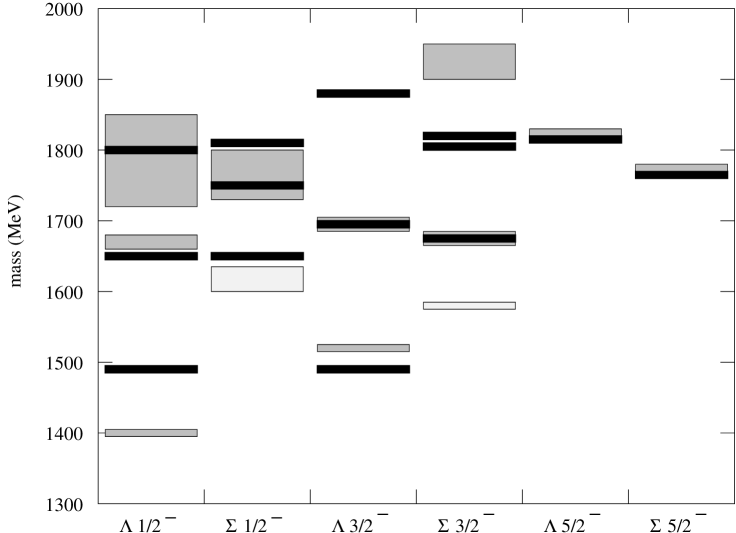
FIG. 4.: The hyperfine perturbation applied to the P-wave strangeness $-1$ baryons. Isgur-Karl model predictions are shown as bars, the range of central values of the masses quoted by the PDG are shown as shaded boxes with 3 and 4* states shaded darker than 2* states.

The $\Sigma{\textstyle{3\over 2}}^{-}$ sector is problematic; Isgur and Karl find a dominantly (quark) spin-${\textstyle{1\over 2}}$ state coinciding with a well established $D_{13}$ state at 1670 MeV which is found to also be dominantly spin-${\textstyle{1\over 2}}$ in the analyses of Faiman and Plane [36] and Hey, Litchfield and Cashmore [35]. The model also predicts a pair of degenerate states at around 1810 MeV. In addition to the $\Sigma(1670)$, there are two $D_{13}$ states extracted from the analyses [3], one poorly established state with two stars at 1580 MeV, and another with three stars at 1940 MeV. The situation appears better for the $\Sigma{\textstyle{1\over 2}}^{-}$ sector, although only one state is resolved at higher mass mass where the model predicts two, and there is no information from the analyses of Refs. [35, 36] about the composition of the lighter state.

The largest problem with the spectrum in Figure 4 is the prediction for the mass of the well-established $\Lambda{\textstyle{1\over 2}}^{-}(1405)$ state, i.e. essentially degenerate with that of the lightest $\Lambda{\textstyle{3\over 2}}^{-}$ state which corresponds to the $\Lambda{\textstyle{3\over 2}}^{-}(1520)$. Isgur and Karl note that the composition essentially agrees with the analyses of Refs. [35, 36]. It is possible that the mass of the lightest $\Lambda{\textstyle{1\over 2}}^{-}$ bound state should be shifted downwards by its proximity to the $\bar{K}N$ threshold, essentially by mixing with this virtual decay channel to which it is predicted to strongly couple. One interaction which can split the lightest $\Lambda{\textstyle{1\over 2}}^{-}$ and $\Lambda{\textstyle{3\over 2}}^{-}$ states is the spin-orbit interaction. Isgur and Karl deliberately neglect these interactions, as their inclusion spoils the agreement with the spectrum in other sectors, for example the masses of the light P-wave nonstrange baryons.

Dalitz[3] reviews the details of the analyses leading to the properties of the $\Lambda{\textstyle{1\over 2}}^{-}(1405)$ resonance, leading to the conclusion that the data can only be fit with an $S$-wave pole in the reaction amplitudes (30 MeV) below $\bar{K}N$ threshold. He discusses two possibilities for the physical origin of this pole: a three quark bound state similar to the one found above, coupled with the S-wave meson-baryon systems; or an unstable $\bar{K}N$ bound state. If the former the problem of the origin of the splitting between this state and the $\Lambda(1520)$ is unresolved. Flavor-dependent interactions between the quarks such as those which result from the exchange of an octet of pseudoscalar mesons between the quarks [37] do not explain the $\Lambda(1520)-\Lambda(1405)$ splitting. If the latter, another state at around 1520 MeV is required and this region has been explored thoroughly in $\bar{K}N$ scattering experiments with no sign of such a resonance.

An interesting possibility is that the reality is somewhere between these two extremes. The cloudy bag model calculations of Veit, Jennings, Thomas and Barrett[38, 39] and Jennings [40] allow these two types of configuration to mix and find an intensity of only 14% for the quark model bound state in the $\Lambda(1405)$, and predict another $\Lambda{\textstyle{1\over 2}}^{-}$ state close to the $\Lambda(1520)$. However, Leinweber [41] obtains a good fit to this splitting using QCD sum rules. Kaiser, Siegel and Weise [42] examine the meson-baryon interaction in the $K^{-}p$, $\Sigma\pi$, and $\Lambda\pi$ channels using an effective chiral Lagrangian. They derive potentials which are used in a coupled-channels calculation of low-energy observables, and find good fits to the low-energy physics of these channels, including the mass of the $\Lambda(1405)$. This important issue will be revisited later when discussing spin-orbit interactions.

B positive-parity excited baryons in the Isgur-Karl model

In order to calculate the spectrum of excited positive-parity nonstrange baryon states, Isgur and Karl [29] construct zeroth-order harmonic-oscillator basis states from spatial states of definite exchange symmetry at the N=2 oscillator level. The details of this construction are given in Appendix A. In this sector both the anharmonic perturbation and the hyperfine interaction cause splittings between the states.

The anharmonic perturbation is assumed to be a sum of two-body forces $U=\sum_{i<j}U_{ij}$, and since it is flavor independent and a spin-scalar, it is SU(6) symmetric. This means that it causes no splittings within a given SU(6) multiplet, which is one of the reasons for classifying the states using SU(6). It does, however, break the initial degeneracy within the N=2 harmonic oscillator band. The anharmonicity is treated as a diagonal perturbation on the energies of the states, and so is not allowed to cause mixing between the $N=0$ and $N=2$ band states. It causes splittings between the $N=1$ band states only when the quark masses are unequal; the diagonal expectations of $U$ in the $N=0$ band (and $N=1$ band for the $N$ and $\Delta$ states) are lumped into the band energies.

For $N$ and $\Delta$ states the symmetry of the states can be used to replace $U=\sum_{i<j}U_{ij}$ by $3U(r_{12})$, where ${\bf r}_{12}={\bf r}_{1}-{\bf r_{2}}=\sqrt{2}\mbox{\boldmath$\rho$}$, and the spin-independent potential is assumed to be a sum of two-body terms. Defining the moments $a$, $b$, and $c$ of the anharmonic perturbation by

$$\left\{a,b,c\right\}:=3{\alpha^{3}\over\pi^{\textstyle{3\over 2}}}\int d^{3}\mbox{\boldmath$\rho$}\left\{1,\alpha^{2}\rho^{2},\alpha^{4}\rho^{4}\right\}U(\sqrt{2}\rho)e^{-\alpha^{2}\rho^{2}},$$ (51)

it is straightforward to show that, the $[56,0^{+}]$ ground states are shifted in mass by $a$, and the $[70,1^{-}]$ states are shifted by $a/2+b/3$ in first order in the perturbation $U$. The states in the $N=2$ band are known [43, 44] to be split into a pattern which is independent of the form of the anharmonicity $U$. This pattern is illustrated in Figure 5, with the definitions $E_{0}=3m+3\omega+a$, $\Omega:=\omega-a/2+b/3$ and $\Delta:=-5a/4+5b/3-c/3$, where $m$ the nonstrange quark mass and $\omega$ the oscillator energy. Isgur and Karl [29] fit $\Omega$ and $\Delta$ to the spectrum of the positive-parity excited states, using $E_{0}=1150$ MeV, $\Omega\simeq 440$ MeV, $\Delta\simeq 440$ MeV, which moves the first radial excitation in the $[56^{\prime},0^{+}]$, assigned to the Roper resonance $N(1440)$, below the (unperturbed by $H^{\rm hyp}$) level of the P-wave excitations in the $[70,1^{-}]$. Note that $\omega$ is 250 MeV, which makes this first order perturbative treatment questionable (since $\Delta\simeq\Omega>\omega$). Also, the off-diagonal matrix elements between the $N=0$ and $N=2$ band states which are present in second order tend to increase the splitting between these two bands. Richard and his collaborators [45] have shown that, within a certain class of models, it is impossible to have this state lighter than the $P$-wave states of Fig. 3 in a calculation which goes beyond first order wave function perturbation theory.

FIG. 5.: The first-order anharmonic perturbation $U$ applied to the nonstrange oscillator basis. The parameters $E_{0}$, $\Omega$, and $\Delta$ are defined in the text.

Diagonalization of the hyperfine interaction of Eq. (19) within the harmonic oscillator basis described in Appendix A results in the energies for nonstrange baryons states shown in Figure 6. The agreement with the masses of the states extracted from data analyses is rather good, with some exceptions. Obviously the model predicts too many states compared with the analyses–several predicted states are ‘missing’. This issue will be discussed in some detail in the section on decays that follows. It will be shown there that Koniuk and Isgur’s model [46] of strong decays, which uses the wave functions resulting from the diagonalization procedure above, establishes that the states seen in the analyses are those which couple strongly to the $\pi N$ (or $\bar{K}N$) formation channel, an idea examined in detail earlier by Faiman and Hendry [47]. It will be shown that this is also verified in some other models which are able to simultaneously describe the spectrum and strong decays.

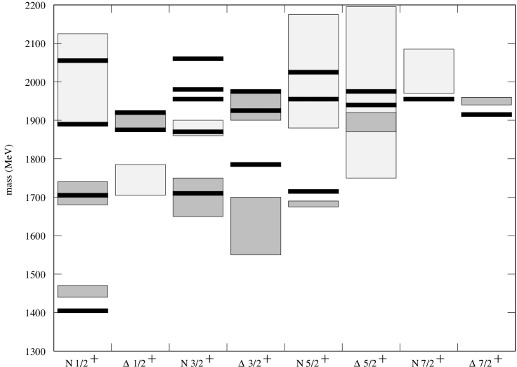
FIG. 6.: The anharmonic and hyperfine perturbations applied to the positive-parity excited nonstrange baryons. Isgur-Karl model predictions are shown as bars, the range of central values of the masses quoted by the PDG are shown as shaded boxes with 3 and 4* states shaded darker than 1 and 2* states.

Figure 6 shows that the predicted mass for the lightest excited $\Delta{\textstyle{3\over 2}}^{+}$ state is higher than that of the lightest $P_{33}$ excited state seen in the analyses, although two recent multi-channel analyses [48, 49] have found central mass values between about 1700 and 1730 MeV, at the high end of the range shown in Fig. 6. The weakly established (1*) $\Delta{\textstyle{1\over 2}}^{+}$ state $\Delta(1750)$ also does not fit well with the predicted model states. Elsewhere the agreement is good.

Masses for positive-parity excited $\Lambda$ and $\Sigma$ states are also calculated by Isgur and Karl in Ref. [29]. The construction of the wave functions for these states is simpler than that of the symmetrized states detailed in Appendix A, as antisymmetry is only required under exchange of the two light quarks. Figures 7 and 8, which show the Isgur-Karl model fit to the the masses of all $\Lambda$ and $\Sigma$ resonances extracted from the data below 2200 MeV, show that the fit for strange positive-parity states is of similar quality to that of the nonstrange positive-parity states, although there are considerably fewer well established experimental states. Once again many more states are predicted than are seen in the analyses. Using the simple selection rule for excited hyperon strong decays described above as a rough guide, Isgur and Karl show [29] that there is a good correspondence in mass between states found in analyses of $\bar{K}N$ scattering data and those predicted to couple to this channel. This strong decay selection rule is modified by configuration mixing in the initial and final states, and so these decays have been examined using subsequent strong decay models which take into account this mixing [46].

FIG. 7.: The anharmonic and hyperfine perturbations applied to the negative and positive-parity excited $\Lambda$ baryons. Isgur-Karl model predictions are shown as bars, the range of central values of the masses quoted by the PDG are shown as shaded boxes with 3 and 4* states shaded darker than 1 and 2* states. Note that the negative-parity and positive-parity states were fit independently.

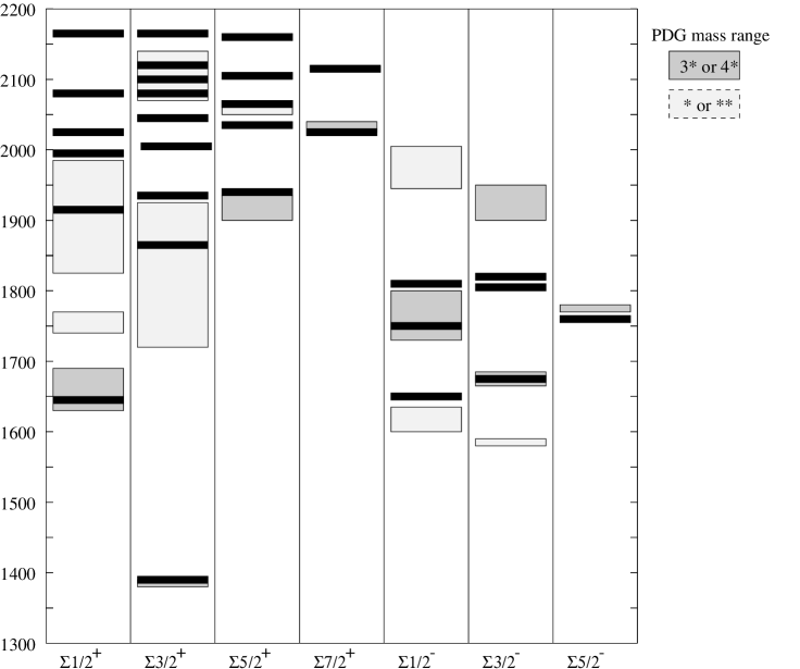
FIG. 8.: The anharmonic and hyperfine perturbations applied to the negative and positive-parity excited $\Sigma$ baryons. Caption as in Fig. 7.

C criticisms of the nonrelativistic quark model

The previous sections show that the main features of the spectrum of the low-lying baryon resonances are quite well described by the nonrelativistic model. Just as importantly, the mixing of the states caused by the hyperfine tensor interaction is crucial to explaining their observed strong decays, e.g. the $N\eta$ decays of the $N^{*}{\textstyle{1\over 2}}^{-}$ states. However, there are several criticisms which can be made of the model. In strongly bound systems of light quarks such as the baryons considered above, where $p/m\simeq 1$, the approximation of nonrelativistic kinematics and dynamics is not justified. For example, if one forms the one-gluon exchange T-matrix element without performing a nonrelativistic reduction, factors of $m_{i}$ in Eq. (19) are replaced, roughly, with factors of $E_{i}=\sqrt{{\bf p}_{i}^{2}+m_{i}^{2}}$. In a potential model picture there should also be ‘kinematic’ smearing of the interquark coordinate ${\bf r}_{ij}$ due to relativistic effects, with a characteristic size given by the Compton wavelength of the quark $1/m_{q}$. A partially relativistic treatment like that of the MIT bag model would at first seem preferable, but problems imposed by restriction to motion within a spherical cavity and in dealing with center of mass motion in this model have not allowed progress to be made in understanding details of the physics of the majority of excited baryon states.

Neglecting the scale dependence of a cut-off field theory (QCD) has resulted in non-fundamental values of parameters like the quark mass, the string tension (implicit in the size of the anharmonic perturbations) and the strong coupling $\alpha_{s}\simeq 1$. A consistent theory with constituent quarks should give those quarks a commensurate size, which will smear out the interactions between the quarks. The string tension should be consistent with meson spectroscopy, and the relation between the anharmonicity and the meson string tension should be explored. If there are genuine three-body forces in baryons, they have been neglected. The neglect of spin-orbit interactions in the Hamiltonian is also inconsistent, independent of the choice of ansatz for the short-distance and confining physics. There is some evidence in the observed spectrum for spin-orbit splittings, e.g. that between the states $\Delta{\textstyle{1\over 2}}^{-}(1620)$ and $\Delta{\textstyle{3\over 2}}^{-}(1700)$, and between $\Lambda{\textstyle{3\over 2}}^{-}(1520)-\Lambda{\textstyle{1\over 2}}^{-}(1405)$, although the latter is likely complicated by decay channel couplings. It is also inconsistent to neglect the various spin-independent but momentum-dependent terms in the Breit-Fermi reduction of the one-gluon-exchange potential.

The model also uses a first-order perturbative evaluation of large perturbations. The contact term is, unless the above smearing is implemented, formally infinite. As shown above, the size of the first-order anharmonic splitting of the $N=2$ band must be larger than the 0-th order harmonic splitting, to get the lightest $N=2$ band nucleon [identified with the Roper resonance $N(1440)$] below the $P$-wave non-strange states. This calls into question the usefulness of first order perturbation theory. It also means that the wave functions of states like the Roper resonance should have a large anharmonic mixing with the ground states. There are also some inconsistencies between the parameters used in describing the negative and positive-parity excited states, which presumably can be traced back to this source.

IV Recent models of excited baryon spectra

A relativized quark model

Several potential model calculations [50, 51, 52, 53, 54] which retain the one-gluon exchange picture of the quark-quark interactions have gone beyond Isgur and Karl’s model for the spectrum and wave functions of baryons in an attempt to correct the flaws in the nonrelativistic model described above. A representative example is the relativized quark model, first applied to meson spectroscopy by Godfrey and Isgur [55], and later adapted to baryons [56]. In this model the Schrödinger equation is solved in a Hilbert space made up of dressed valence quarks with finite spatial extent and masses of 220 MeV for the light quarks, and 420 MeV for the strange quark. The Hamiltonian is now given by

$$H=\sum_{i}\sqrt{{\bf p}_{i}^{2}+m_{i}^{2}}+V,$$ (52)

where $V$ is a relative-position and -momentum dependent potential which tends, in the nonrelativistic limit (which is not taken here) to the sum

$$\lim_{p_{i}/m_{i}\to 0}V=V_{\rm string}+V_{\rm Coul}+V_{\rm hyp}+V_{\rm so(cm)}+V_{\rm so(Tp)}.$$ (53)

The terms are a confining string potential, a pairwise color-Coulomb potential, a hyperfine potential, and spin-orbit potentials associated with one-gluon exchange and Thomas precession in the confining potential. The momenta $p_{i}$ are written in terms of the momenta ${\bf p}_{\rho}$, ${\bf p}_{\lambda}$ conjugate to the Jacobi coordinates of Eq. (30) and the total momentum ${\bf P}$, in order to separate out the center of mass momentum. Note that spin-independent but momentum-dependent terms present in O$(p^{2}/m^{2})$ reduction of the one-gluon-exchange potential are omitted here.

The gluon fields are taken to be in their adiabatic ground state, and generate a confining potential $V_{\rm string}$ in which the quarks move. This is effectively linear at large separation and can be written as the sum $V_{\rm string}=\sum_{i}b\,l_{i}+C$ of the energies of strings of length $l_{i}$ connecting quark $i$ to a string junction point, where $b$ is the meson string tension. The string is assumed to adjust infinitely quickly to the motion of the quarks so that it is always in its minimum length configuration; this generates a three-body adiabatic potential for the quarks [58, 59, 50, 60, 54] which includes genuine three-body forces.

The Coulomb, hyperfine, color-magnetic and Thomas-precession spin-orbit potentials are as they were in the nonrelativistic model [25, 28, 29] except that: (1) the inter-quark coordinate ${\bf r}_{ij}$ is smeared out over mass-dependent distances, as suggested by relativistic kinematics and QCD; (2) the momentum dependence away from the $p/m\to 0$ limit is parametrized, as suggested by relativistic dynamics. In practice, (1) is brought about by convoluting the potentials with a smearing function $\rho_{ij}({\bf r}_{ij})=\sigma_{ij}^{3}e^{-\sigma_{ij}^{2}r_{ij}^{2}}/\pi^{3\over 2}$, where the $\sigma_{ij}$ are chosen to smear the inter-quark coordinate over distances of O(1/$m_{Q}$) for Q heavy, and approximately 0.1 fm for light quarks; (2) is brought about by introducing factors which replace the quark masses $m_{i}$ in the nonrelativistic model by, roughly, $E_{i}$. For example the contact part of $H^{ij}_{\rm hyp}$ becomes

$$V^{ij}_{\rm cont}=\left({m_{i}m_{j}\over E_{i}E_{j}}\right)^{{1\over 2}+\epsilon_{\rm cont}}{8\pi\over 3}\alpha_{s}(r_{ij}){2\over 3}{{\bf S}_{i}\cdot{\bf S}_{j}\over m_{i}m_{j}}\left[{\sigma_{ij}^{3}\over\pi^{3\over 2}}e^{-\sigma_{ij}^{2}r_{ij}^{2}}\right]\left({m_{i}m_{j}\over E_{i}E_{j}}\right)^{{1\over 2}+\epsilon_{\rm cont}},$$ (54)

where $\epsilon_{\rm cont}$ is a constant parameter, and $\alpha_{s}(r_{ij})$ is a running-coupling constant which runs according to the lowest-order QCD formula, saturating to 0.6 at $Q^{2}=0$.

The energies and wave functions of all the baryons are then solved for by expanding the states in a large harmonic oscillator basis. Wave functions are expanded to $N\leq 7$ ($N\leq 8$ for $J^{P}={\textstyle{1\over 2}}^{+}$). The Hamiltonian matrix is diagonalised in this basis, and energy eigenvalues are then crudely minimized in $\alpha$, the harmonic-oscillator size parameter. To avoid construction of symmetrized wave functions in this large basis, the non-strange wave functions are not explicitly antisymmetrized in $u$ and $d$ quarks. Instead, the strong Hamiltonian (which cannot distinguish $u$ and $d$ quarks) is allowed to sort the basis into $N$ and $\Delta$ states.

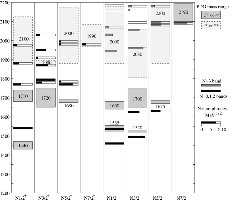
FIG. 9.: Mass predictions and $N\pi$ decay amplitudes (whose square is the $N\pi$ decay width) for nucleon resonances below 2200 MeV from Refs. [56, 61], compared to the range of central values for resonances masses from the PDG [3], which are shown as boxes. The boxes are lightly shaded for one and two star states and heavily shaded for 3 and four star states. Predicted masses are shown as a thin bar, with the length of the black shaded region indicating the size of the $N\pi$ amplitude. The ground state nucleon mass from this model is 960 MeV.

The resulting fit to the masses of excited nucleon states below 2200 MeV is compared to the range of central values for resonances masses in that mass range from the PDG [3] in Figure 9. In addition, Fig. 9 illustrates the results for the $N\pi$ decay amplitudes of these states of a strong decay calculation based on the creation of a pair of quarks with ${}^{3}P_{0}$ quantum numbers [61]. The length of the shaded region in the bar representing the model state’s mass is proportional to the size of the $N\pi$ decay amplitudes, which when squared gives the partial width to decay to $N\pi$. This is so that states which are likely to have been seen in analysis of elastic and inelastic $\pi N$ scattering can be identified among the states predicted by the model. Figure 10 illustrates the same quantities for excited $\Delta$ states. Figures 11 and 12 compare the fit to the excited $\Lambda$ and $\Sigma$ states below 2200 MeV to the range of central values for resonance masses in that mass range, which are extracted from analyses of $\bar{K}N$ and other scattering experiments listed in the PDG [3].

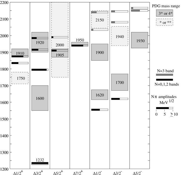
FIG. 10.: Model masses and $N\pi$ decay amplitudes for $\Delta$ resonances below 2200 MeV from Refs. [56, 61], compared to the range of central values for resonances masses from the PDG [3]. Caption as in Fig. 9.

The pattern of splitting in the negative and positive-parity bands of excited nonstrange states is reproduced quite well, although the centers of the bands are missed by about $-50$ MeV and $+50$ MeV, respectively. The Roper resonance mass is about 100 MeV too high compared to the nucleon ground state, but fits well into the pattern of splitting of the positive-parity band. This problem is slightly worse in the case of the state $\Delta{\textstyle{3\over 2}}^{+}(1600)$. The negative-parity $\Delta$ states in the $N=3$ band are too high when compared to the masses of a well-established pair of resonant states $\Delta{\textstyle{1\over 2}}^{-}(1900)$ and $\Delta{\textstyle{3\over 2}}^{-}(1930)$. It is clear from Figs. 11 and 12 that the relativized model does not have the freedom that the nonrelativistic model has to fit the mass splittings caused by the strange-light quark mass difference in the negative-parity strangeness $-1$ baryons. The pattern of splitting in the positive-parity strangeness $-1$ baryons is reproduced well, with again the band being predicted too heavy by about 50 MeV.

It has been shown by Sharma, Blask, Metsch and Huber [57] that the inclusion of the spin-independent but momentum-dependent terms present in an O($p^{2}/m^{2}$) reduction of the one-gluon exchange potential reduces the energy of certain positive-parity excited states, and raises that of the P-wave excited states. It is possible that the inclusion of such terms in the Hamiltonian of Eq. (52) could explain the roughly $\pm 50$ MeV discrepancy between the relativized model masses of these bands of states and those extracted from the analyses.

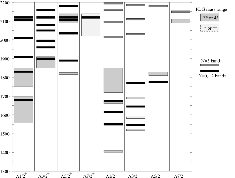
FIG. 11.: Model masses for $\Lambda$ resonances below 2200 MeV from Ref. [56], compared to the range of central values for resonances masses from the PDG [3], which are shown as boxes. The boxes are lightly shaded for one and two star states and heavily shaded for 3 and four star states. Model masses are shown as a thin bar. The ground state $\Lambda$ mass in this model is 1115 MeV.

The model of Ref. [56] shows some improvements, and some deterioration relative to the nonrelativistic model, largely because it does not contain the freedom to separately fit the negative-parity and positive-parity states present in the nonrelativistic model. The same set of parameters is used to fit all mesons [55] and baryons, except the string tension $b$ is reduced about 15% from the meson value in the best fit of Ref. [56]. Spin-orbit interactions in this model are small, for several reasons; a smaller $\alpha_{s}$ is used, while retaining the same contact interaction splittings, by virtue of the non-perturbative evaluation of the expectation value of the smeared contact interaction. Perturbative evaluation of a $\delta$-function contact term underestimates the size of the contact splittings, and so requires a larger value of $\alpha_{s}$ to compensate, which increases the size of the OGE spin-orbit interactions. There is also, as expected [28], a partial cancellation of the color-magnetic and Thomas-precession spin-orbit terms, and freedom present in the model to choose $\epsilon_{\rm cont}<\epsilon_{\rm so}$ to suppress the spin-orbit interactions relative to the hyperfine terms has been exploited.

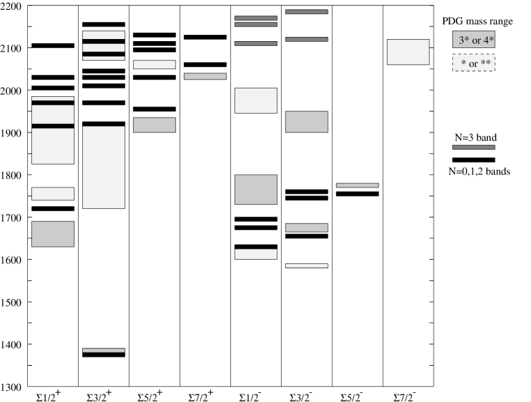
FIG. 12.: Model masses for $\Sigma$ resonances below 2200 MeV from Ref. [56], compared to the range of central values for resonances masses from the PDG [3]. Caption as in Fig. 11. The ground state $\Sigma$ mass in this model is 1190 MeV.

B semirelativistic flux-tube model

A parallel extension of one-gluon-exchange (OGE) based models was carried out by Sartor and Stancu [54], and by Stancu and Stassart [62, 63]. The spin-independent part of the interquark Hamiltonian contains a relativistic kinetic energy term and the string confining potential, as well as a pairwise color-Coulomb interaction between the quarks. The hyperfine interaction has a spin-spin contact term and a tensor interaction which are properly smeared out over the finite size of the constituent quark. In contrast to the use of a harmonic-oscillator basis in the relativized model, this work uses a variational wave function basis first employed by Carlson, Kogut and Pandharipande (CKP) [60]. This basis essentially interpolates between Coulomb and linear potential solutions, and contains a factor which decreases as the length of the Y-shaped string connecting the quarks increases. This allows the use of a significantly smaller set of basis states than the oscillator basis used by other authors, because the large distance behavior of the wave functions is closer to that of the true eigenstates. On the other hand, it is somewhat more complicated to work with, especially in momentum space. Sartor and Stancu [54] extend the calculation of CKP by calculation of the hyperfine interaction between the quarks. This model is used by these authors to carry out an extensive survey of baryon strong decay couplings, which is described in detail below.

C models based on instanton-induced interactions

An alternate QCD-based candidate for the short-range interactions between quarks is that calculated by ’t Hooft [64, 65, 66] from instanton effects. This interaction is flavor-dependent, and was originally designed to solve the $\pi$-$\eta$-$\eta^{\prime}$ puzzle which exists in quark models of mesons based on one-gluon exchange. An expansion of the Euclidean action around single-instanton solutions of the gauge fields assuming zero-mode dominance in the fermion sector leads to an effective contact interaction between quarks, which acts only if the quarks are in a flavor anti-symmetric state. The color structure requires that the quarks be in an anti-triplet of color, which is always true of a pair of quarks in the ground state antisymmetric color configuration of a baryon. The strength of the interaction is proportional to a divergent interaction which must be regularized, and so is usually taken to be an adjustable constant. In the nonrelativistic approximation this leads to an interaction between quarks in a baryon which has nonzero matrix elements [67]

$$\langle q^{2};S,L,T|W|q^{2};S,L,T\rangle=-4g\,\delta_{S,0}\,\delta_{L,0}\,\delta_{T,0}\cal{W}$$ (55)

of the interaction $W$, where ${\cal W}$ is the radial matrix element of the contact interaction. Note that the interaction acts only on pairs in a spin singlet, S-wave, isospin-singlet state. Although not present in the one-loop calculation of ’t Hooft, higher-order calculations are expected to regularize the $\delta$-function contact interaction to yield

$$\delta^{3}({\bf r})\to{1\over\Lambda^{3}\pi^{3/2}}e^{-r^{2}/\Lambda^{2}},$$ (56)

so that the radial matrix elements ${\cal W}$ are finite.

This interaction can be extended to encompass the interactions between three flavors of quark, with the result that they are completely antisymmetric in flavor space. An additional parameter $g^{\prime}$ is required for the strength of the effective interaction between nonstrange and strange quarks. The result is an interaction between quarks with three parameters $g$, $g^{\prime}$ and $\Lambda$ that causes no shifts of the masses of decuplet baryon states, but shifts octet flavor states downward if they contain spin-singlet, S-wave, flavor-antisymmetric pairs.

Ground-state baryon mass splittings with instanton-induced interactions are explored in a simple model by Shuryak and Rosner [68], and in the MIT bag model by Dorokhov and Kochelev [69] and Klabučar [70]. Dorokhov and Kochelev’s model also included OGE-based interactions. An extensive study of the meson and baryon spectra using a string-based confining interaction and instanton-induced interactions is made by Blask, Bohn, Huber, Metsch, and Petry (BBHMP) [67]. Evidence for the role of instantons in determining light-hadron structure and quark propagation in the QCD vacuum is given by Chu, Grandy, Huang, and Negele [71] in their study based on lattice QCD.

The nonrelativistic model of BBHMP [67] confines the quarks in mesons and baryons using a string potential of the kind proposed by Carlson, Kogut and Pandharipande [53]. In addition, it has only instanton-induced interactions between the quarks, and is applied to baryons and mesons of all flavors made up of $u$, $d$, and $s$ quarks. The model has only eight parameters which are the three quark masses, the string tension, two energy offset parameters for mesons and baryons, and the three parameters $g$, $g^{\prime}$ and $\Lambda$ of the instanton-induced interactions. It is able to explain the sign and rough size of the splittings in the ground state baryons, and also the size of the splittings in certain P-wave baryons, such as the $N$ and $\Lambda$ states are described well. The splittings in the $P$-wave $\Sigma$ states are smaller than the (less certain) splittings extracted from experiment. Positive-parity excited states tend to be too massive by about 200-250 MeV. Nevertheless, given the simplicity of the model, the authors have demonstrated the possibility that instanton-induced interactions may play an important role in the determination of the spectrum of light hadrons.

D Goldstone-boson exchange models

Many authors have proposed that because of the special nature of the pion, and to a lesser extent the other members of the octet of pseudoscalar mesons, one should consider the exchange of pions between light quarks in nucleon and $\Delta$ baryons as a source of hyperfine interactions. The best developed early exploration of the consequences of this for the baryon spectrum is by Robson [72]. Glozman and Riska have popularized this idea by making an extensive analysis of the baryon spectrum using a model based on a hyperfine interaction arising solely from the exchange of a pseudoscalar octet. They argue that, contrary to the substantial evidence presented in the prior literature, there is no evidence for a one-gluon-exchange hyperfine interaction. For a comprehensive review of this work, see Ref. [73]. More recently Glozman, Plessas, Varga and Wagenbrunn [74, 75, 76] (for the most recent version of this model see Ref. [77]) have extended this model to include the exchange of a nonet of vector mesons and a scalar meson, and the calculation of radial matrix elements of the exchange potentials.

To illustrate the argument used by these authors, consider Fig. 13 from Ref. [77].

FIG. 13.: Low-lying spectra of nucleon, $\Delta$ and $\Lambda$ states from Ref. [77].

The argument is that the order of the states extracted from the analyses is inverted in the $N$, $\Delta$, and $\Lambda$ spectra compared to the ($+,-,+$) ordering of the levels using either harmonic or linear confinement. Of course this ordering can be perturbed by the one-gluon exchange interaction, and in the case of linear confinement the splitting between the negative-parity and positive-parity excited states becomes smaller, but it is still not possible to lower with the hyperfine contact interaction the mass of the lightest positive-parity $N{\textstyle{1\over 2}}^{+}$ excited state below that of the lightest negative-parity $N{\textstyle{1\over 2}}^{-}$ state (see, for example, Fig. 9). For the $\Delta$ states the one-gluon exchange OGE interaction shifts the radially excited $\Delta{\textstyle{3\over 2}}^{+}$ state up relative to the negative parity excited states $\Delta{\textstyle{1\over 2}}^{-}$ and $\Delta{\textstyle{3\over 2}}^{-}$. It is argued that this points conclusively to a flavor-dependence of the hyperfine interaction, and that the best candidate for such an interaction is Goldstone-boson exchange (GBE). Note that the situation becomes less clear if one admits that the masses of these resonances, which are extracted from difficult analyses which do not always agree, have a range of possible values. For example, the range in masses quoted by the PDG [3] for the state ‘$\Delta{\textstyle{3\over 2}}^{+}(1600)$’ is 1550 to 1700 MeV, with more recent analyses [48, 49] at the upper end of this range. Similarly the state $\Lambda{\textstyle{1\over 2}}^{+}(1600)$ has a mass range of 1560-1700 MeV. In both cases the greater uncertainty on the mass of the positive-parity state means that it could have a mass roughly the same as, or higher than, the negative parity states. As we have seen above, there is also another QCD-based candidate for a flavor-dependent force between quarks, which is that arising from instanton effects.

In Ref. [73] the flavor-dependent spin-spin force has the form

$$H_{\chi}\sim-\sum_{i<j}\frac{V({\bf r}_{ij})}{m_{i}m_{j}}\mbox{\boldmath$\lambda$}^{\rm F}_{i}\cdot\mbox{\boldmath$\lambda$}^{\rm F}_{j}\,\mbox{\boldmath$\sigma$}_{i}\cdot\mbox{\boldmath$\sigma$}_{j},$$ (57)

where $\mbox{\boldmath$\lambda$}^{\rm F}_{i}$ is a Gell-Mann matrix in the flavor space and the radial dependence of the function $V({\bf r}_{ij})$ is assumed to be unknown. This interaction can be made to roughly fit the pattern of mass splittings of Figure 13 in a model with harmonic confinement by choosing 5 parameters, which are the harmonic oscillator excitation energy $\omega$, and four radial matrix elements of the pion exchange radial function $V^{\pi}({\bf r}_{ij})$. The fitted mass differences are those between the nucleon and $\Delta{\textstyle{3\over 2}}^{+}(1232)$, $N{\textstyle{1\over 2}}^{+}(1440)$, and $\Delta{\textstyle{3\over 2}}^{+}(1600)$, as well as the average masses of the two pairs of states $N{\textstyle{1\over 2}}^{-}(1535)$–$N{\textstyle{3\over 2}}^{-}(1520)$, and $N{\textstyle{3\over 2}}^{+}(1720)$–$N{\textstyle{5\over 2}}^{+}(1680)$. Four further parameters are used in the fit to other nonstrange baryon states (up to N=2 in the harmonic oscillator spectrum), which are the radial matrix elements of the $\eta$-exchange radial potential between light quarks $V^{uu}({\bf r}_{ij})$, for a total of nine parameters.

The size of the resulting harmonic oscillator energy $\omega\simeq 160$ MeV is considerably smaller than that required in the Isgur-Karl model. This acts to lower the splittings between the harmonic-oscillator levels prior to application of the spin-spin force. The difference between the oscillator frequencies in the $\rho$ and $\lambda$ systems is neglected.

In fitting to the strange baryon masses twelve new parameters are required, which are the four radial matrix elements of the kaon-exchange potential $V^{K}({\bf r}_{ij})$, and the light-strange and strange-strange $\eta$-exchange radial potentials $V^{us}({\bf r}_{ij})$ and $V^{ss}({\bf r}_{ij})$. The difference between the oscillator frequencies in the $\rho$ and $\lambda$ systems is neglected, which amounts to the adoption of a flavor-dependent confining force. This gives a total of 23 parameters, including the values of the quark masses $m_{u}=340$ MeV and $m_{s}=461$ MeV, used to fit the spectrum of $N$, $\Delta$, $\Lambda$, $\Sigma$, $\Xi$, and $\Omega$ baryons up to the $N=2$ band. Given the large number of parameters the work reviewed in Ref. [73] can be considered a demonstration that a flavor-dependent contact interaction in Eq. (57) can be used to fit the spectrum.

Calculations now exist which go beyond a parametrization of the spectrum in terms of GBE, and have included vector and scalar meson exchanges [75, 74, 76]. In this work the relativistic quark kinetic energy $\sum_{i}\sqrt{{\bf p}_{i}^{2}+m_{i}^{2}}$ is used, as well as a pairwise linear confining interaction with a strength $C=0.46$ GeV/fm. It can be shown that the sum of interquark separations $\sum_{i<j=1}^{3}r_{ij}$ and the sum of the string lengths in a Y-shaped string connecting the quarks differ by about a factor of 0.55 in $S$-states [56]. This means that this linear potential strength is reasonable compared to the string tension of 1 GeV/fm found in lattice calculations. Note, however, that a string model of the confining potential contains genuine three-body forces which are not in a pairwise linear potential. The Schrödinger equation is solved using a variational calculation in a large harmonic oscillator basis as in Ref. [56]. Tensor interactions which are associated with the GBE contact interactions as well as scalar and vector meson exchanges are now included. The primary motivation for this appears to be that certain tensor mixings change sign when going from vector exchange (like OGE) to GBE, and this makes problematic the strong decays [75] and nucleon form factors [79] in a GBE model based only on pseudoscalar exchange. There are now separate exchange potentials for a pseudoscalar nonet ($\pi$, $K$, $\eta$ and $\eta^{\prime}$), a vector meson nonet ($\rho$, $K^{*}$, $\omega_{8}$ and $\omega_{0}$) and a singlet scalar meson ($\sigma$).

The result is a complicated model with on the surface a large amount of freedom to fit the spectrum, since associated with each of the seventeen exchanged particles is a coupling constant $g_{\gamma}$, and a (monopole) meson-quark form factor parameter $\Lambda_{\gamma}$. In addition each of the vector mesons couples with a second coupling constant, i.e. there are two constants $g^{V}_{\gamma}$ and $g^{T}_{\gamma}$ for each vector meson. A range parameter $1/\mu_{\gamma}$ is presumably fixed by making $\mu_{\gamma}$ the exchanged particle’s mass in the case of physical mesons. In earlier calculations without the vector and scalar exchanges the number of parameters is reduced by assuming that the form factor parameters scale with meson mass as $\Lambda_{\gamma}=\Lambda_{0}+\kappa\mu_{\gamma}$, and by adopting only two coupling constants $g_{8}$ and $g_{0}$ for the octet and singlet ($\eta^{\prime}$) members of the pseudoscalar nonet. It is not clear from Refs. [76, 77] how many parameters are used in the most recent calculations of this group.

Potentials are now given the form expected from a nonrelativistic reduction of the $T$-matrix element for exchange of the corresponding meson, and matrix elements of these potentials are calculated in the harmonic oscillator basis rather than parametrized. Note that the momentum-dependence of the (Yukawa-like) exchange potentials is still that given by the nonrelativistic limit, which is somewhat inconsistent as the quarks exchanging the mesons are off-shell. The results for the spectrum of $N$, $\Delta$ and $\Lambda$ baryons up to spin-${\textstyle{5\over 2}}$ (predictions for ${\textstyle{7\over 2}}^{+}$ baryons are absent) are shown in Figure 14, and those for $\Sigma$, $\Xi$ and $\Omega$ baryons are shown in Figure 15. It is not explained in Refs. [76, 77] how model states which are expected to appear in analyses of the data are chosen to compare with the spectrum of such states from the PDG. Recent work within the GBE model [74, 75, 76, 77] does not include ${\textstyle{7\over 2}}^{+}$ baryon states as well as other higher-lying missing states because the authors believe that in this mass region both the constituent quark model and a potential model of confinement are not adequate [78].

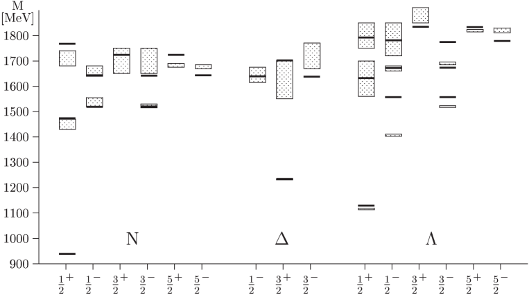
FIG. 14.: Energy levels of low-lying $N$, $\Delta$ and $\Lambda$ baryons from Refs. [76, 77], compared to the range of central values for resonances masses from the PDG [3].

An extension of the model to include strong decays to $N\pi$, $\Delta\pi$ and $N\eta$ [75] has been made using emission of point-like (elementary) pions and etas (an elementary emission model), and the pseudoscalar exchange potentials to describe the masses. The resulting description of the decay widths is described by the authors as not consistent. The authors attribute this to the lack of meson structure, and also the lack of configuration mixing caused by tensor interactions, both of which are shown below to be important for a model of baryon strong decays. Recent calculations [80] use the ${}^{3}P_{0}$ model described below for the strong couplings and the pseudoscalar, vector and scalar potentials to determine the masses, but have not included the tensor interactions. The tensor force from pseudoscalar exchange and that from pseudoscalar, vector and scalar exchanges is qualitatively different, so exploring its consequences for strong decays in this model is important.

Given the amount of freedom in the model to fit the spectrum, it is perhaps not surprising that the fit is of somewhat better quality than that of the relativized model of Ref. [56], which uses 13 parameters to fit the nonstrange baryon spectrum, eight of which are the same as those used in a similar fit to meson physics [55]. Note that because of the special status given to mesons, it is not clear whether a unified picture of baryons and mesons could ever emerge in the GBE model. Although the mass of the first recurrence of $\Delta{\textstyle{3\over 2}}^{+}$ is now above 1700 MeV (at the top end of the range quoted by the PDG) and heavier than the negative-parity $\Delta$ states, presumably because of the effects of the exchange of vector quantum numbers (like that of OGE), this is still somewhat lighter than the relativized model mass of $\simeq 1800$ MeV. The Roper resonance can be made lighter than the $P$-wave $N$ and $\Delta$ resonances. The equivalent $\Lambda{\textstyle{1\over 2}}^{+}$ state is still somewhat heavier than the $\Lambda{\textstyle{1\over 2}}^{-}$–$\Lambda{\textstyle{3\over 2}}^{-}$ pair, which are predicted degenerate at about 1550 MeV.

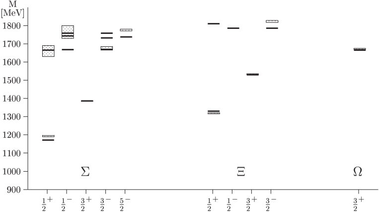
FIG. 15.: Energy levels of low-lying $\Xi$ and $\Omega$ baryons from Ref. [76, 77]. Caption as in Fig. 14.

E spin-orbit interactions in baryons

As shown above, it is inconsistent to simply ignore the spin-orbit interactions which are associated with the one-gluon exchange interaction postulated in several models as the source of the hyperfine splitting in baryons. There also exist purely kinematical spin-orbit interactions associated with Thomas precession of the quark spins in the confining potential which must be taken into account. Are spin-orbit interactions present in baryons, with a strength commensurate with the vector-exchange contact interaction and the confining interaction? Isgur and Karl [25] calculate the size of these interactions, and show that under certain reasonable conditions on the potentials, a cancellation of the vector and scalar spin-orbit interactions occurs for the two-body parts of the spin-orbit interactions. Note that this cancellation relies on the Lorentz structure of the confining interaction being a scalar. However, in a three-body system there are also spin-orbit interactions involving, say, the orbital angular momentum of the 1-2 quark pair and the spin of the third quark which have no analogue in bound states of two particles. There is no cancellation between the three-body spin orbit interactions arising from these two sources. Inclusion of all of these spin-orbit forces still leads to unacceptably large spin-orbit splittings, and so Isgur and Karl leave them out. There is also some evidence for spin-orbit splittings in the analyses of the data, for example the splitting $\Delta{\textstyle{3\over 2}}^{-}-\Delta{\textstyle{1\over 2}}^{-}$ in Fig. 3. Leaving these interactions out is unsatisfactory.

In the relativized model the contact interaction is evaluated nonperturbatively, and the usual $\delta^{3}({\bf r}_{ij})$ form is smeared out by relativistic effects and the finite size of the constituent quarks. The perturbative evaluation of the $\delta^{3}({\bf r}_{ij})$ interaction in the nonrelativistic model underestimates its strength; in the relativized model for the same contact splitting a value of $\alpha_{s}=0.6$ is required, significantly smaller than that required in the nonrelativistic model. The result is a smaller associated spin-orbit interaction. Some of the freedom to fit the momentum dependence of the potentials is used to further suppress the spin-orbit interactions relative to the contact interaction. These effects, along with a partial cancellation of the vector and scalar spin-orbit terms (the latter are calculated with a two-body approximation to the string confining potential) reduce the size of the spin-orbit interactions to acceptable levels. This calculation shows that it is possible to construct a model based on one-gluon exchange in which spin-orbit interactions are treated consistently and still adequately fit the spectrum.

In these models the splitting between $\Lambda{\textstyle{3\over 2}}^{-}(1520)$ and $\Lambda{\textstyle{1\over 2}}^{-}(1405)$ can arise only from a spin-orbit interaction, if  no mass shifts arising from decay-channel couplings [or $qqq(\bar{q}q)$ configurations] are allowed. In the relativized model there is very little splitting of these two states from the spin-orbit interaction. The presence of the nearby threshold for $N\bar{K}$ decay is expected to strongly affect the mass of $\Lambda{\textstyle{1\over 2}}^{-}(1405)$. Obviously any  model which ignores the effects of decay-channel couplings will not be able to fully explain this splitting. As mentioned above, the cloudy bag model calculations of Veit, Jennings, Thomas and Barrett[38, 39] and Jennings [40] allow an unstable $\bar{K}N$ bound state to mix with a three-quark bound state and find that the low mass of the $\Lambda(1405)$ can be explained by a small (14%) intensity for the quark model bound state in the $\Lambda(1405)$. This model predicts another $\Lambda{\textstyle{1\over 2}}^{-}$ state close in mass to the $\Lambda(1520)$ in a region where one has not been seen.

In a calculation of baryon masses based on QCD sum rules, Leinweber [41] finds a large spin-orbit splitting in the $\Lambda{\textstyle{3\over 2}}^{-}(1520)$–$\Lambda{\textstyle{1\over 2}}^{-}(1405)$ system while maintaining a small splitting in the $N{\textstyle{3\over 2}}^{-}(1520)$–$N{\textstyle{1\over 2}}^{-}(1535)$ system. A simple approximate formula for the ratio of the masses of the $J^{P}={\textstyle{1\over 2}}^{-}$ states is derived that gives $\Lambda{\textstyle{1\over 2}}^{-}/N{\textstyle{1\over 2}}^{-}=\langle\bar{s}s\rangle/\langle\bar{u}u\rangle$, which shows that the $\Lambda{\textstyle{1\over 2}}^{-}(1405)$ becomes lighter than the $N{\textstyle{1\over 2}}^{-}(1535)$ because of the reduced size of the strange quark condensate in this approach. Note that the mechanism by which the two nucleon states remain degenerate in mass while the two $\Lambda$ states become split is apparently complicated. Although the splittings of the above states are described rather well, theoretical errors are substantial compared to the spin-orbit splittings. Furthermore, because of the complexity of this approach, only six baryon states are considered (the four $P$-wave states above and the ground state nucleon and $\Lambda$) and all of the nucleon states are calculated to be 50-75 MeV too light, whereas the calculated $\Lambda$ state masses are within 25 MeV of the physical masses. The central result is that, in this approach, the large $\Lambda$ spin-orbit splitting is not due to coupling to the $\bar{K}N$ scattering channel, but rather to the reduced strange quark condensate relative to the $u$ or $d$ condensates. This is in contrast to the cloudy-bag [38, 39, 40] and chiral potential model [42] descriptions of the $\Lambda(1405)$ detailed above.

The development by Glozman and Riska (see Refs. [73, 77] and references therein) of a model for nonstrange and strangeness -1 baryon masses with hyperfine interactions induced by Goldstone-boson-exchange (GBE) between the quarks was partially motivated by the lack of associated spin-orbit interactions. It is claimed that this supports the hypothesis that the hyperfine interactions responsible for many features of the baryon spectrum are due to GBE and not one-gluon exchange (OGE). However, as pointed out by Isgur [81], it is still necessary to confine the quarks in such a model. Glozman and Riska use harmonic confinement, although more recent calculations [74, 76] have used linear confinement, and as noted above such confining forces produce spin-orbit interactions through Thomas precession. Isgur argues that, in addition to the usual problems with the three-body spin-orbit interactions, the cancellation of the two-body components of the Thomas-precession spin-orbit forces which can be arranged with the OGE hyperfine interaction will be spoiled with GBE hyperfine interactions. This is precisely because the two-body spin-orbit interactions which usually arise from the hyperfine interaction are not present. Isgur points out that with OGE such a cancellation is able to explain the small size of spin-orbit interactions in mesons.

In a recent paper on meson-like $\Lambda^{*}_{Q}$ baryons, where $Q$ is a heavy quark, Isgur [82] shows that their spin-independent spectra are remarkably like those of the analogous mesons. Such states have orbital angular momentum only between the light-quark pair and the heavy quark $Q$, so that the only spin-orbit forces are those on the heavy quark $Q$. Spin-orbit interactions in such states are shown to be small due to a cancellation between one-gluon exchange and Thomas-precession spin-orbit forces which occurs with the assumption of Lorentz scalar confinement. For such states the three-body spin-orbit interactions from the OGE and confining interactions conspire to produce only meson-like quasi-two-body spin-orbit forces. Isgur also argues that the states ${}^{2}\Sigma^{*}_{Q}$ and ${}^{4}\Lambda^{*}_{Q}$ have the same spatial wave function as $\Lambda^{*}_{Q}={{}^{2}\Lambda}^{*}_{Q}$, so that in these states the spin-orbit forces on the heavy quark $Q$ (which are not the only such forces present) also exhibit this cancellation. He concludes that a careful reanalysis of spin-orbit splittings is required, since a nonrelativistic solution to the size of the spin-orbit splittings in mesons and $\Lambda^{*}_{Q}$ states is possible, although it is still possible that relativistic effects have produced a gross enhancement of spin-spin over spin-orbit interactions in baryons, as suggested in Ref. [56].

F diquark and collective models

Models of baryon structure exist which describe the nucleon (for a review see Anselmino et al. [83]) and its excitations [84] in terms of a diquark and a quark. If the diquark is tightly bound its internal excitation is costly in energy, so that the low-lying excitations of the nucleon will not include excitations of the diquark. Early models assumed that, because of an attractive hyperfine interaction between a $u$ and $d$-quark in the isospin-zero spin-zero channel, there should be a tightly-bound isoscalar scalar diquark in the proton and other baryons. In SU(6) language this means that, in addition to the lightest negative-parity nonstrange excitations in the [70,1^-] multiplet which have all been seen in $N\pi$ elastic scattering, the low-lying positive-parity nonstrange excitations of the nucleon should lie in symmetric 56-plet and mixed-symmetry 70-plet representations. Models which treat all three quarks symmetrically have more low-lying excitations. Light positive-parity excited states are present in the [56^′,0⁺], [70,0⁺], [56,2⁺], [70,2⁺], and [20,1⁺] SU(6) multiplets, with $J^{P}=1/2^{+}$, $3/2^{+}$, $5/2^{+}$, and $7/2^{+}$, for a total of twenty-one positive-parity nonstrange excited states. Note that some diquark models also allow for the quark and diquark to interact and exchange a quark and so their identity in order to maintain overall antisymmetry [84], and may have similar numbers of positive-parity excited states, although the [20,1⁺] multiplet is still excluded.

Of the twenty-one low-lying positive-parity nonstrange excited states predicted by symmetric quark models, nine are considered well established by the Particle Data Group (PDG) [3], there are three tentative (one or two stars) nucleon states, and two tentative $\Delta$ states, for a total of fourteen, of which five need confirmation. The remaining predicted states can be defined as missing [46]. This definition can be expanded to include any baryon predicted by symmetric quark models but noticeably absent in the analyses, such as the many higher mass negative-parity states above 1900 MeV. Although not discussed in detail here, the situation is similar for the strange baryons $\Lambda$ and $\Sigma$, except there are fewer excited states present in the analyses, with a few missing low-lying negative-parity states and more missing positive-parity states.

These states may be missing because of strong diquark clustering in the light-quark baryons. There is some evidence from the lattice [85] and from an analysis of baryon strong decays [86] that such strong diquark clustering may not be present. The explanation adopted here, and in the work of others [46], is that such states have either small $N\pi$ couplings in a partial wave which includes other light strongly coupled states, or are close in mass to a more strongly coupled state, both of which make extraction of a signal from $N\pi$ elastic scattering difficult. This explanation can be understood using a quark model of the spectrum and wave functions of these states and their strong decay, which are described below. This model can then be used to show how such states can be found.

A collective model of baryon masses, electromagnetic couplings, and strong decays based on a spectrum-generating algebra has been developed by Bijker, Iachello and Leviatan (BIL) [87, 88, 89]. The idea is to extend the algebraic approach, which led to the mass formulae based on flavor-spin symmetry described above, to the description of the spatial structure of the states. The quantum numbers of the states are considered to be distributed spatially over a Y-shaped string-like configuration, which is sometimes idealized as being a thin string with a distribution of mass, charge and magnetic moments. BIL also apply their algebraic model to a single-particle valence quark picture for comparison purposes.

The approach to the dynamics is not the usual solution of some Schrödinger-like equation, but rather bosonic quantization of the spatial degrees of freedom, which in this case are the two relative coordinates $\rho$ and $\lambda$ of Eq. (30). This leads to six vector boson operators bilinear in the components of these coordinates and their conjugate momenta, plus an additional scalar boson, which generate the Lie algebra of U(7). This means that the spectrum-generating algebra of the baryon problem is taken to be U(7)$\otimes$SU(3)${}_{\rm f}\otimes$SU(2)${}_{\rm spin}\otimes$SU(3)_c.

Bases are constructed by operating with the boson operators on the vacuum. Mass and electromagnetic coupling calculations require construction of a complete set of basis states for representations of U(7), and these are obtained by considering subalgebras. A basis corresponding to two coupled three-dimensional harmonic oscillators, corresponding to the nonrelativistic and relativized quark models, is used for the mass calculations. A second basis corresponding to a three-dimensional oscillator and a three-dimensional Morse oscillator coupled together is more convenient for evaluation of the electromagnetic coupling strengths.

All mass operators can then be expanded into elements of U(7) which transform as irreducible representations of the rotation group SO(3) and exchange symmetry $S_{3}$. Instead of expanding the Hamiltonian used in other approaches, the mass-squared operator is expanded in terms of operators of the algebra U(7), which is appropriate for a relativistic system. For identical constituents, the mass-squared operator is constrained to be symmetric under the exchange group. BIL then write down the most general mass-squared operator which is a scalar under rotations and the exchange group and which preserves parity, and which is at most quadratic in the elements of U(7). For strange baryons a more general operator which is not necessarily symmetric under the exchange group $S_{3}$ is employed. The masses and wave functions corresponding to this mass operator are then found by diagonalization in either of the two bases described above.

By choosing coefficients of the tensor structures in the mass-squared operator, BIL are able to make contact with harmonic oscillator quark models, although these are usually written for the mass and not the mass squared. They are also able to describe collective (string-like) models with the three constituents moving in a correlated way. For the latter model, the mass-squared operator is rewritten to describe vibrations and rotations of the string-like configuration. The vibrational part of the mass-squared operator has fundamental vibrational modes which correspond to breathing and bending modes of the strings. The rotational part does not reproduce the linear rise of the mass squared with orbital angular momentum (linear Regge trajectories) which is approximately reproduced by using a linear potential and a relativistic kinetic energy operator in the usual quark potential models. A more complicated alternate form for the rotational part of the mass-squared operator is constructed to reproduce this behavior, in terms of the orbital angular momentum and its projection onto the three-fold symmetry axis of the string configuration. This corresponds to the rotational spectrum of an oblate top. This choice introduces vibration-rotation interactions, which are dropped. Also the part of the rotational term in the mass-squared operator dependent on the projection of the angular momentum onto the symmetry axis is dropped as there is no evidence for such a term in the spectrum.

The resulting orbital spectrum has four parameters which are fit to the spectrum. It describes positive-parity excitations with $L^{P}=0^{+}$ as the lightest of a group of one-phonon vibrational excitations, so that they lie below a parity-doublet of states with $L^{P}=1^{+},1^{-}$. The spin-flavor part of the mass-squared operator is then written in terms of six generators (Casimir operators) of the spin-flavor algebra. All terms which are not in the diagonal part of the operator are dropped. The operator simplifies into three terms (each multiplied by a parameter) in the case of nonstrange baryons, which are the usual spin-spin interaction, a flavor-dependent interaction, and ‘exchange’ terms which depend on the permutation symmetry of the wave functions. Finally, there is the possibility of operators which involve both internal and spatial degrees of freedom such as the hyperfine tensor and spin-orbit interactions. These interactions are not considered, which has consequences for the electromagnetic and strong decay amplitudes calculated with the eigenstates of this mass-squared operator.

The result of the choices outlined above, some of which have been made with the spectrum in mind, is a mass-squared operator with seven parameters which are fit to the nonstrange baryon spectrum. The spin-orbit problem, described in detail above, is simply avoided by leaving out such interactions. The ‘exchange’ terms in the general form of the spin-flavor dependent part of the mass operator are found to be crucial to fitting the higher unperturbed position of the P-wave baryons relative to the ground state and positive-parity excited states, which was put in by hand in the Isgur-Karl model (see Fig. 9) and remains a problem at the $\simeq$100 MeV level in the relativized model. As is the case with the relativized models of Refs. [55, 56], there is consistency between the slope of the Regge trajectory and of the spin-spin interactions found here and in mesons [90]. This model predicts more missing baryons, with different quantum numbers and masses, than the valence quark models. The lightest of the missing nucleon states are two states in an antisymmetric $[20,1^{+}]$ multiplet at 1720 MeV, with $J^{P}={\textstyle{1\over 2}}^{+}$ and ${\textstyle{3\over 2}}^{+}$. The presence of these states is an easily testable consequence of this model, as their presence is predicted in addition to the model states assigned to the resonances $N{\textstyle{1\over 2}}^{+}(1710)$ and $N{\textstyle{3\over 2}}^{+}(1720)$ seen in the analyses. It is also necessary to show that these light missing states couple relatively weakly to the $\pi N$ formation channel in a strong-decay analysis to explain why they have not been seen. In Ref. [89] these states are shown to have zero partial widths into all strong decay channels considered ($N\pi$, $N\eta$, $\Sigma K$, $\Lambda K$, and $\Delta\pi$). However, if there are present tensor (or spin-orbit) interactions these will cause mixings with nearby states which should allow these (presumably quite narrow) states to be seen. It is also possible that these states decay to channels not considered by BIL and likely to contain missing baryons, like $N\rho$.

The resulting spectrum of nucleon and $\Delta$ states is shown in Figs. 16 and 17. Only those model states below 2 GeV are shown, although the plots go to higher energies to display the errors on the states seen in the analyses. Model states which have been assigned to resonant states from the analyses are distinguished from ‘missing’ states by having darker-shaded bars representing the mass predictions. The model is able to fit the mass of the Roper resonance, and correctly fit the centers of gravity of the P-wave and low-lying positive-parity states, due to the additional ‘exchange’ terms in the mass-squared operator. The lightest $N{\textstyle{7\over 2}}^{-}$ state is 150-200 MeV too light compared to the four star state $N{\textstyle{7\over 2}}^{-}(2190)$, and from the less certain extractions of masses of other multiply-excited negative-parity states, it appears that this entire band of nucleon states is generally predicted too light.

FIG. 16.: Mass predictions for nucleon states from the collective algebraic model of Bijker, Iachello, and Leviatan [87], shown as bars, compared to the range of central values for resonances masses from the PDG [3], which are shown as boxes. Model states which are assigned to experimental states by virtue of their masses and decay couplings are shown as darker-shaded bars, ‘missing’ states as lighter shaded bars. The ground state nucleon mass from this model is 939 MeV.

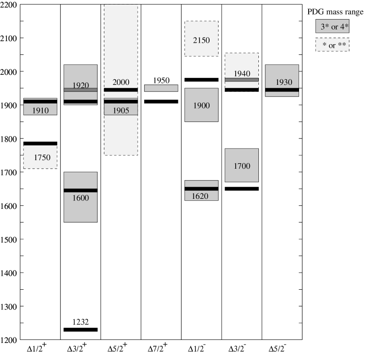
FIG. 17.: Mass predictions for $\Delta$ states from the collective algebraic model of Bijker, Iachello, and Leviatan [87], shown as bars, compared to the range of central values for resonances masses from the PDG [3], which are shown as boxes. Caption as in Fig. 16.

Although an extension of this model involving four extra parameters to the $\Lambda$, $\Sigma$, $\Xi$ and $\Omega$ baryons has very recently been made by BIL [89], space does not allow a description of the results of this calculation here, except that the fit is of comparable quality and that the model also predicts more missing strange baryons than valence quark models. Strong decays in the BIL model are described in detail below.

G P-wave nonstrange baryons in large $N_{c}$ QCD

Recently Carlson, Carone, Goity, and Lebed [91, 92] have examined the masses of the nonstrange P-wave baryons using a mass operator analysis in large $N_{c}$ QCD. The approach is to write down all possible independent operators which could appear in the effective mass operator, and order those operators by their size in a $1/N_{c}$ expansion. The result is that the mass operator contains, for two quark flavors, 18 spin-singlet flavor-singlet operators to order $N_{c}^{-2}$. As there are seven masses and two mixing angles (those between the two $N{\textstyle{1\over 2}}^{-}$ states and the two $N{\textstyle{3\over 2}}^{-}$ states), the hierarchy in $1/N_{c}$ is initially used to select a set of nine operators which are able to efficiently describe these quantities. In Ref. [91] it is found that only a few of the coefficients in the effective Hamiltonian turn out to be of natural size, with the rest being small or consistent with zero. Further operator analysis in Ref. [92] allows fits to be made just to the masses, and the resulting fit can be used to predict the mixing angles. An adequate fit can be made using just three operators, although this fit does not give the best results for the mixing angles. The set of three operators have quantum numbers consistent with single-pion exchange between the quarks, but are not easily compatible with other simple models such as OGE.

H hybrid baryon masses

Current experiments which search for new baryons using electromagnetic probes, such as those in Hall B at TJNAF, will also produce hybrid baryon states. These are states which are described in quark potential models as having explicit excitation of the gluon degrees of freedom. Low-lying baryon states present in analyses of $\pi N$ elastic and inelastic scattering, such as the Roper resonance $N{\textstyle{1\over 2}}^{+}(1440)$, have been proposed [93, 94, 95, 96] as hybrid candidates. This is based on extensions of the MIT bag model [97, 98, 99, 100] to states where a constituent gluon in the lowest energy transverse electric mode combines with three quarks in a color octet state to form a colorless state, and on a calculation using QCD sum rules [95, 96]. Hybrid baryons have also been constructed recently in the large-$N_{c}$ limit of QCD [101].

With the assumption that the quarks are in an S-wave spatial ground state, and considering the mixed exchange symmetry of octet color wave functions of the quarks, bag-model constructions show that adding a $J^{P}=1^{+}$ gluon to three light quarks with total quark-spin 1/2 yields both $N$ ($I=\frac{1}{2}$) and $\Delta$ ($I=\frac{3}{2}$) hybrids with $J^{P}=\mbox{$\textstyle\frac{1}{2}$}^{+}$, $\mbox{$\textstyle\frac{3}{2}$}^{+}$. Quark-spin 3/2 hybrids are $N$ states with $J^{P}=\mbox{$\textstyle\frac{1}{2}$}^{+}$, $\mbox{$\textstyle\frac{3}{2}$}^{+}$, and $\mbox{$\textstyle\frac{5}{2}$}^{+}$. Energies are estimated using the usual bag Hamiltonian plus gluon kinetic energy, additional color-Coulomb energy, and one-gluon exchange plus gluon-Compton O($\alpha_{s}$) corrections. Mixings between $q^{3}$ and $q^{3}g$ states from gluon radiation are evaluated. If the gluon self-energy is included, the lightest $N$ hybrid state has $J^{P}=\frac{1}{2}^{+}$ and a mass between that of the Roper resonance and the next observed $J^{P}=\mbox{$\textstyle\frac{1}{2}$}^{+}$ state, $N{\textstyle{1\over 2}}^{+}(1710)$. A second $J^{P}=\frac{1}{2}^{+}$ $N$ hybrid and a $J^{P}=\frac{3}{2}^{+}$ $N$ hybrid are expected to be 250 MeV heavier, with the $\Delta$ hybrid states heavier still. A similar mass estimate of about 1500 MeV for the lightest hybrid is attained in the QCD sum rules calculation of [95, 96].

These results are interesting, given the controversial nature of the Roper resonance and its $\Delta{\textstyle{3\over 2}}^{+}(1600)$ equivalent in OGE-based potential models, and the difficulties global models of the electromagnetic couplings of baryons have accommodating the substantial Roper resonance photocouplings. As the $N{\textstyle{1\over 2}}^{+}(1710)$ and its photocouplings are quite well described by conventional models, if the Roper is a hybrid then there should be another $P_{11}$ state in the mass region from 1440-1710 MeV. Evidence for two resonances near 1440 MeV in the $P_{11}$ partial wave in $\pi N$ scattering was cited [102], which would indicate the presence of more states in this energy region than required by the $q^{3}$ model, but this has been interpreted as due to complications in the structure of the $P_{11}$ partial wave in this region [103] (see also Ref. [104]), and not an additional physical state.

A recent calculation [105] of hybrid baryon masses in the flux-tube model [106, 107] finds that the lightest hybrid baryons have similar good quantum numbers, but substantially higher energies and different internal structure than predicted using bag models. This model structure of the glue, where the gluon degrees of freedom collectively condense into flux-tubes, is very different from the constituent-gluon picture of the bag model and large-$N_{c}$ constructions. It is based on an expansion around the strong-coupling limit of the Hamiltonian formulation of lattice QCD, and on the assumption that the dynamics relevant to the structure of hybrids is that of confinement. The dynamics is treated in the adiabatic approximation, where the quarks do not move in response to the motion of the glue (apart from moving as a rigid body in order to maintain the center-of-mass position). Flux lines (strings) with energy proportional to their length play the role of the glue, which are modeled by equal mass beads with a linear potential between nearest neighbors [106, 107]. The total mass of all of the beads is given by the energy in the flux lines, which is fixed by the string tension. Beads are allowed to move in a plane perpendicular to their rest positions.

The ground state energy of this configuration of beads representing the Y-string for definite quark positions ${\bf r}_{i}$ defines an adiabatic potential $V_{B}({\bf r}_{1},{\bf r}_{2},{\bf r}_{3})$ for the quarks, which consists of the string energy $b\sum_{i}l_{i}$, where $b$ is the string tension and $l_{i}$ is the magnitude of the vector ${\bf l}_{i}$ from the equilibrium junction position to the position of quark $i$, plus the zero-point energy of the beads. The energy of the first excited state defines a new adiabatic potential $V_{H}({\bf r}_{1},{\bf r}_{2},{\bf r}_{3})$. It is shown in Ref. [105] that a reasonable approximation to the string ground state and first excited state adiabatic surfaces may be found by allowing only the junction to move, while the strings connecting the junction to the quarks follow without excitation. These adiabatic surfaces are found numerically via a variational calculation. Hybrid baryon masses are then found by allowing the quarks to move in a confining potential given by the linear potential $b\sum_{i}l_{i}$, plus $V_{H}-V_{B}$, with the rest of the dynamics as in the relativized model calculation of [56] except that spin-dependent terms are neglected. When added to the spin-averaged mass of the $N$ and $\Delta$ which is 1085 MeV, hybrids with quark orbital angular momenta $L_{q}=0,1,2$ have masses 1980, 2340 and 2620 MeV respectively. Hyperfine (contact plus tensor) interactions split the $N$ hybrids down and the $\Delta$ hybrids up by similar amounts, so that the $N$ hybrid mass becomes 1870 MeV. The error in this mass, due to uncertainties in the parameters, is estimated to be less than $\pm 100$ MeV. This lightest ($L_{q}=0$) hybrid level is substantially higher than the roughly 1.5 GeV estimated from bag model and QCD sum rules calculations.

Taking into account the exchange symmetry and angular momentum of the excited string, the calculation of Ref. [105] finds that the lightest hybrid baryons are $N{\textstyle{1\over 2}}^{+}$ and $N{\textstyle{3\over 2}}^{+}$ states with quark spin of ${\textstyle{1\over 2}}$ and masses of around 1870 MeV. The $\Delta{\textstyle{1\over 2}}^{+}$, $\Delta{\textstyle{3\over 2}}^{+}$ and $\Delta{\textstyle{5\over 2}}^{+}$ hybrids have quark spin of ${\textstyle{3\over 2}}$ and masses of around 2090 MeV. The lightest nucleon states are in the region of the ‘missing’ $P_{11}$ and $P_{13}$ resonances predicted by most models. Of course there will be mixing between conventional excitations (based on the glue in its ground state) and these hybrid states, so it is expected that the physics of the $N{\textstyle{1\over 2}}^{+}$ and $N{\textstyle{3\over 2}}^{+}$ baryons in the 1700-2000 MeV region will be complicated. Nevertheless, a careful examination of the states in this region, with multiple formation and decay channels, may turn up evidence for these new kinds of excitations.

V Baryon electromagnetic couplings

In Born approximation, single-pion photoproduction involves a combination of an electromagnetic (EM) excitation process for an excited baryon and a strong decay (in the $s$ and $u$ channels), or a meson EM transition in the $t$ channel (see Figure 18). In addition, a contact diagram is required to maintain gauge invariance in a nonrelativistic treatment. Data for this process have been analyzed to come up with a set of photocouplings, which give the strength of electromagnetic transitions $\gamma N\to X$ between the nucleons and excited baryon states. To do this, the magnitude of the strong decay amplitudes are divided out of the product $A_{\gamma N\to X}\cdot A_{X\to N\pi}$, to form the quantity

$${A_{\gamma N\to X}\cdot A_{X\to N\pi}\over|A_{X\to N\pi}|}$$ (58)

which is inclusive of the phase of the amplitude $A_{X\to N\pi}$, which cannot be measured in $\pi N$ elastic scattering. It is these amplitudes which are quoted as photocouplings in the PDG [3]. The calculation of these strong decay amplitudes will be detailed below, and this can be used to find a set of signs of these amplitudes for a given spectral model and set of wave functions. Here the calculation of EM excitation amplitudes in the nonrelativistic model is outlined, and a fit of such a model to the values for these photocouplings extracted from analyses of the data is examined.

FIG. 18.: Born diagrams for pion photoproduction.

Evaluation of the strength of electromagnetic transitions $\gamma N\to X$ between the nucleons and excited baryon states involves finding matrix elements of an EM transition Hamiltonian between states in the harmonic-oscillator basis, and is similar to the evaluation of the interquark Hamiltonian described above.

The idea is to use the impulse approximation, illustrated in Figure 19, which describes the target nucleon and the final resonance as made up of quarks which are free while interacting with the photon, but whose momenta, charges and spins are distributed according to the bound-state wave functions which result from a model of the spectrum.

FIG. 19.: The impulse approximation for the electromagnetic interaction.

A nonrelativistic model

The EM interaction Hamiltonian can be found from a nonrelativistic reduction of the quark current $e^{i(p^{\prime}-p)\cdot x}{\bar{u}}(p^{\prime},s^{\prime})[-ie\gamma^{\mu}]u(p,s)$ to be

$$H^{\rm em}=\sum_{i}H^{\rm em}_{i}=-\sum_{i}\left\{{e_{i}\over 2m_{i}}\left[{\bf p}_{i}\cdot{\bf A}({\bf r}_{i})+{\bf A}({\bf r}_{i})\cdot{\bf p}_{i}\right]+\mbox{\boldmath$\mu$}_{i}\cdot\mbox{\boldmath$\nabla$}_{i}\times{\bf A}({\bf r}_{i})\right\},$$ (59)

where $\mbox{\boldmath$\mu$}_{i}=e_{i}\mbox{\boldmath$\sigma$}_{i}/2m_{i}$ is the magnetic moment of the $i$-th quark, $e_{i}$, $m_{i}$, $\mbox{\boldmath$\sigma$}_{i}/2$, ${\bf p}_{i}$ are its charge, (constituent) mass, spin, and momentum, and ${\bf A}$ is the photon field. The term quadraric in ${\bf A}$ is important for Compton scattering but does not affect the tree-level quark-photon vertex. Note that this interaction is flavor dependent, even for equal mass quarks, through its dependence on the charge $e_{i}$, so amplitudes for production from the proton and neutron contain independent information about the structure of the initial and final baryons.

There are, in general, a pair of amplitudes $A_{1/2}$ and $A_{3/2}$ associated with photoproduction from each target, which correspond to the two possibilities for aligning the spin of the photon and initial baryon in the center of momentum (c.m.) frame. This is illustrated in Figure 8 for photoproduction of a $\Delta{\textstyle{3\over 2}}^{+}$ state; note only $A_{1/2}$ is needed to describe photoproduction of baryons $X$ with $J_{X}=1/2$. These helicity amplitudes are defined in terms of helicity states by

$$A^{N}_{\lambda}=\langle XJ_{X};{\bf 0}\lambda|H^{\rm em}|N{\textstyle{1\over 2}};-{\bf k}\lambda_{N}\rangle,$$ (60)

where $\lambda_{N}=\lambda_{\gamma}-\lambda=1-\lambda$ if ${\bf k}\parallel\hat{\bf z}$, and $N=p,n$. Eq. (60) is specialized to the case of photoproduction of the nonstrange baryons $N$ and $\Delta$ for which the bulk of the analyzed data exists, although the generalization to the unequal mass case, e.g. for radiative decays of excited hyperons [108], is straightforward.

FIG. 20.: Momenta and helicities in the center of momentum frame for photoproduction of $\Delta{\textstyle{3\over 2}}^{+}$; (a) defines the amplitude $A_{1/2}$, and (b) defines $A_{3/2}$.

To reduce the $H^{\rm em}$ of Eq. (59) to an operator which acts between a nucleon and a resonance wave function, first substitute the monochromatic photon field

$${\bf A}_{\bf k}({\bf r}_{i})=\sum_{\lambda}\sqrt{2\pi\over k_{0}}\left(\mbox{\boldmath$\epsilon$}_{{\bf k},\lambda}e^{i{\bf k}\cdot{\bf r}_{i}}a_{{\bf k},\lambda}+\mbox{\boldmath$\epsilon$}^{*}_{{\bf k},\lambda}e^{-i{\bf k}\cdot{\bf r}_{i}}a^{{\dagger}}_{{\bf k},\lambda}\right),$$ (61)

where $k_{0}=|{\bf k}|$ for real photons, and then use the first (photon absorption) part with $\mbox{\boldmath$\epsilon$}_{{\bf k},+1}=-(1,i,0)/\sqrt{2}$, and choose ${\bf k}\parallel{\hat{\bf z}}$. It is possible, when calculating the photocouplings of the $N$ and $\Delta$ resonances, to exploit the overall symmetry of the wave functions (without the color wave function) to make the replacement $H^{\rm em}\to 3H^{\rm em}_{3}$. This is a convenient choice, since for the equal mass case the momentum of the third quark is just ${\bf p}_{3}=\sqrt{2/3}{\bf p}_{\lambda}+{\bf P}/3$, where the momenta ${\bf p}_{\rho}$ and ${\bf p}_{\lambda}$ have equivalent definitions to their conjugate coordinates $\rho$ and $\lambda$, and ${\bf P}$ is the total momentum.

The result of inserting plane waves for the center of mass motion of the baryons and integrating over the position coordinates is

$$A^{N}_{\lambda}=3\langle XJ;\lambda|-{e_{3}\over 2m_{u}}{1\over\sqrt{2}}\sqrt{2\pi\over k_{0}}e^{-ik\sqrt{2\over 3}\lambda_{z}}\left(\sqrt{2\over 3}p_{\lambda+}-k{\sigma_{3+}\over 2}\right)|N{\textstyle{1\over 2}};\,\lambda-1\rangle.$$ (62)

Here $p_{\lambda+}=p_{\lambda x}+ip_{\lambda y}$, and $\sigma_{3+}$ raises the spin of the third quark. The expectation value in Eq. (62) is best carried out in momentum space, where the recoil phase factor has the effect of shifting the ${\bf p}_{\lambda}$ momentum of the final-state wave function by $\sqrt{2/3}{\bf k}$.

The helicity amplitudes for photoproduction of any excited $\Delta(I={\textstyle{3\over 2}})$ state satisfy $A^{p}_{\lambda}=A^{n}_{\lambda}$, since the expectation values of the charge operator $e_{3}$ between the flavor wave functions for the $N$ and $\Delta$ satisfy

$$\langle\phi^{S}_{\Delta^{+}}|e_{3}|\phi^{\rho}_{p}\rangle = \langle\phi^{S}_{\Delta^{0}}|e_{3}|\phi^{\rho}_{n}\rangle=0$$ (63)

$$\langle\phi^{S}_{\Delta^{+}}|e_{3}|\phi^{\lambda}_{p}\rangle = \langle\phi^{S}_{\Delta^{0}}|e_{3}|\phi^{\lambda}_{n}\rangle=-\sqrt{2}e/3,$$ (64)

where $e$ is the proton charge.

Koniuk and Isgur [46] calculated the amplitudes of Eq. (62) using the Isgur-Karl model [25, 28, 29] wave functions, which include configuration mixing caused by the hyperfine interaction. In order to compare with the helicity amplitudes quoted in the Particle Data Group (PDG) [3], the sign of the $N\pi$ decay amplitudes must be calculated in the model. The quality of the $\gamma N\to N\pi$ data is poorer than the $N\pi$ elastic data, and so a resonance $X$ must be present in $N\pi$ elastic in order to extract its photocoupling $A^{N}_{\lambda}(X)$. As mentioned above, since the sign of the coupling $A_{X\to N\pi}$ cannot be determined in $N\pi$ scattering, the PDG quote $A^{N}_{\lambda}(X)\cdot A_{X\to N\pi}/|A_{X\to N\pi}|$ for the photocoupling helicity amplitude, i.e. inclusive of the sign of $A_{X\to N\pi}$ (there are also some other conventional signs included, see Ref. [46]).

The results of this calculation, with signs calculated using the elementary emission strong decay model of Ref. [46], are listed for $\Delta(1232)$ and the N=1 band negative-parity nonstrange baryons in Table I, and for the N=2 band positive-parity nonstrange baryons in Table II. Also shown there are the empirical photocouplings extracted for these states from analyses of pion photoproduction data. For most low-lying states the agreement is quite good; for certain well determined states, such as the Roper resonance $N{\textstyle{1\over 2}}^{+}(1440)$, there are sizeable discrepancies. This may be partially due to deficiencies in the wave functions and the nonrelativistic approximation, which is not as well justified when applied to some photocouplings. The photon momentum is determined by conservation of momentum in the excited baryon c.m. frame to be $k=(M_{X}^{2}-m_{N}^{2})/2M_{X}$ at resonance, and is not small compared to the average quark momentum when $M_{X}$ is substantially larger than $M_{N}$. When the struck quark recoils against the other quarks in the baryon with a relativistic momentum, the Galilean momentum shift in Eq. (62) cannot be accurate.

TABLE I.: Photoproduction amplitudes from the fits of Koniuk and Isgur (KI) [46], the fit $A^{M}_{1}$ of Li and Close (LC) [112], the extended-string fit with $R^{2}=1.0$ of Bijker, Iachello and Leviatan (BIL) [87], and the relativized fit of Capstick (SC) [114] for $\Delta(1232)$ and N=1 band baryons, compared to amplitudes extracted from analyses of the data (PWA) [3]. Amplitudes are in units of $10^{-3}$ GeV${}^{-{\textstyle{1\over 2}}}$; a factor of $+i$ is suppressed for all negative-parity states. As BIL do not calculate the sign of $A_{X\to N\pi}$ the signs of their amplitudes are to be used only to compare the relative signs of different amplitudes for the same state.

State	$A^{N}_{\lambda}$	KI	LC	BIL	SC	PWA
$\Delta{\textstyle{3\over 2}}^{+}(1232)$	$A^{p,n}_{\textstyle{1\over 2}}$	$-$103	$-$94	$-$91	$-$108	$-$135$\pm$ 6
	$A^{p,n}_{\textstyle{3\over 2}}$	$-$179	$-$162	$-$157	$-$186	$-$255$\pm$ 8
$N{\textstyle{1\over 2}}^{-}(1535)$	$A^{p}_{\textstyle{1\over 2}}$	+147	+142	+162/+127a	+76	+90$\pm$ 30
	$A^{n}_{\textstyle{1\over 2}}$	$-$119	$-$77	$-$112/$-$103a	$-$63	$-$46$\pm$ 27
$N{\textstyle{1\over 2}}^{-}(1650)$	$A^{p}_{\textstyle{1\over 2}}$	+88	+78	+0/+91a	+54	+53$\pm$ 16
	$A^{n}_{\textstyle{1\over 2}}$	$-$35	$-$47	+25/$-$41a	$-$35	$-$15$\pm$ 21
$\Delta{\textstyle{1\over 2}}^{-}(1620)$	$A^{p,n}_{\textstyle{1\over 2}}$	+59	+72	$-$51	+81	+27$\pm$ 11
$N{\textstyle{3\over 2}}^{-}(1520)$	$A^{p}_{\textstyle{1\over 2}}$	$-$23	$-$47	$-$43	$-$15	$-$24$\pm$ 9
	$A^{p}_{\textstyle{3\over 2}}$	+128	+117	+109	134	+166$\pm$ 5
	$A^{n}_{\textstyle{1\over 2}}$	$-$45	$-$75	$-$27	$-$38	$-$59$\pm$ 9
	$A^{n}_{\textstyle{3\over 2}}$	$-$122	$-$127	$-$109	$-$114	$-$139$\pm$ 11
$N{\textstyle{3\over 2}}^{-}(1700)$	$A^{p}_{\textstyle{1\over 2}}$	$-$7	$-$16	0	$-$33	$-$18$\pm$ 13
	$A^{p}_{\textstyle{3\over 2}}$	+11	$-$42	0	$-$3	$-$2$\pm$ 24
	$A^{n}_{\textstyle{1\over 2}}$	$-$15	+35	+11	18	0$\pm$ 50
	$A^{n}_{\textstyle{3\over 2}}$	$-$76	+10	+57	$-$30	$-$3$\pm$ 44
$\Delta{\textstyle{3\over 2}}^{-}(1700)$	$A^{p,n}_{\textstyle{1\over 2}}$	+100	+81	$-$82	+82	+104$\pm$ 15
	$A^{p,n}_{\textstyle{3\over 2}}$	+105	+58	$-$82	+68	+85$\pm$ 22
$N{\textstyle{5\over 2}}^{-}(1675)$	$A^{p}_{\textstyle{1\over 2}}$	+12	+8	0	+2	+19$\pm$ 8
	$A^{p}_{\textstyle{3\over 2}}$	+16	+11	0	+3	+15$\pm$ 9
	$A^{n}_{\textstyle{1\over 2}}$	$-$37	$-$30	$-$33	$-$35	$-$43$\pm$ 12
	$A^{n}_{\textstyle{3\over 2}}$	$-$53	$-$42	$-$47	$-$51	$-$58$\pm$ 13

^a With the inclusion of a 38^∘ mixing between the $S_{11}$ states (not calculated in the model of BIL).

TABLE II.: Breit frame photoproduction amplitudes for positive parity (N=2 band) excited states for which there exist data. Caption as in Table I.

State	$A^{N}_{\lambda}$	KI	LC	BIL	SC	PWA
$N{\textstyle{1\over 2}}^{+}(1440)$	$A^{p}_{\textstyle{1\over 2}}$	$-$24		0	+4	$-$65$\pm$ 4
	$A^{n}_{\textstyle{1\over 2}}$	+16		0	$-$6	+40$\pm$ 10
$N{\textstyle{1\over 2}}^{+}(1710)$	$A^{p}_{\textstyle{1\over 2}}$	$-$47	$-$18	$-$22	+13	+9$\pm$ 22
	$A^{n}_{\textstyle{1\over 2}}$	$-$21	$-$22	+7	$-$11	$-$2$\pm$ 14
$\Delta{\textstyle{1\over 2}}^{+}(1910)$	$A^{p,n}_{\textstyle{1\over 2}}$	+59	$-$28	+17	$-$8	+3$\pm$ 14
$N{\textstyle{3\over 2}}^{+}(1720)$	$A^{p}_{\textstyle{1\over 2}}$	$-$133	$-$68	+118	$-$11	+18$\pm$ 30
	$A^{p}_{\textstyle{3\over 2}}$	+46	+53	$-$39	$-$31	$-$19$\pm$ 20
	$A^{n}_{\textstyle{1\over 2}}$	+57	$-$4	$-$33	+4	+1$\pm$ 15
	$A^{n}_{\textstyle{3\over 2}}$	$-$10	$-$33	0	+11	$-$29$\pm$ 61
$\Delta{\textstyle{3\over 2}}^{+}(1600)$	$A^{p,n}_{\textstyle{1\over 2}}$	$-$46	$-$38	0	+30	$-$23$\pm$ 20
	$A^{p,n}_{\textstyle{3\over 2}}$	$-$16	$-$70	0	+51	$-$9$\pm$ 21
$\Delta{\textstyle{3\over 2}}^{+}(1920)$	$A^{p,n}_{\textstyle{1\over 2}}$		$-$14	$-$17	+13	40$\pm$ 14a
	$A^{p,n}_{\textstyle{3\over 2}}$		$-$7	+30	+14	23$\pm$ 17
$N{\textstyle{5\over 2}}^{+}(1680)$	$A^{p}_{\textstyle{1\over 2}}$	0	$-$8	$-$4	$-$38	$-$15$\pm$ 6
	$A^{p}_{\textstyle{3\over 2}}$	+91	+105	+80	+56	+133$\pm$ 12
	$A^{n}_{\textstyle{1\over 2}}$	+26	+11	+40	+19	+29$\pm$ 10
	$A^{n}_{\textstyle{3\over 2}}$	$-$25	$-$43	0	$-$23	$-$33$\pm$ 9
$\Delta{\textstyle{5\over 2}}^{+}(1905)$	$A^{p,n}_{\textstyle{1\over 2}}$	+8	+24	$-$11	+26	+26$\pm$ 11
	$A^{p,n}_{\textstyle{3\over 2}}$	$-$33	+25	$-$49	$-$1	$-$45$\pm$ 20
$N{\textstyle{7\over 2}}^{+}(1990)$	$A^{p}_{\textstyle{1\over 2}}$	$-$8		0	$-$1	+15$\pm$ 25b
	$A^{p}_{\textstyle{3\over 2}}$	$-$10		0	$-$2	+45$\pm$ 33
	$A^{n}_{\textstyle{1\over 2}}$	$-$18		+23	$-$15	$-$40$\pm$ 30
	$A^{n}_{\textstyle{3\over 2}}$	$-$23		+29	$-$18	$-$147$\pm$ 45
$\Delta{\textstyle{7\over 2}}^{+}(1950)$	$A^{p,n}_{\textstyle{1\over 2}}$	$-$50	$-$28	+28	$-$33	$-$76$\pm$ 12
	$A^{p,n}_{\textstyle{3\over 2}}$	$-$69	$-$36	+36	$-$42	$-$97$\pm$ 10

^a No signs are extracted for these amplitudes.
^b Average of two existing analyses.

B models with relativistic corrections

The nonrelativistic operator $H^{\rm em}$ adopted above is not expanded to the same order as the interquark Hamiltonian, O$(p^{2}/m^{2})$. To this order spin-orbit interactions must be added, and Brodsky and Primack [109, 110] have shown from the requirement of electromagnetic gauge invariance that there are also associated two-body currents (which go beyond the simple impulse approximation illustrated in Fig. 5). These corrections were put together with the configuration-mixed nonrelativistic wave functions in a calculation of the photocouplings by Close and Li [111, 112], and using the relativized model wave functions described above in the calculation of Capstick [113, 114]. Note that the latter calculation does not ‘relativize’ the O($p^{2}/m^{2}$) electromagnetic interaction Hamiltonian by parametrizing its momentum dependence away from the nonrelativistic limit, although the wavefunctions are generated using a relativized inter-quark potential. These results are compared to the empirical photocouplings extracted from pion photoproduction analyses also shown in Figures 21 and 22. It is clear that these additional effects improve the comparison with the extracted photocouplings, although they clearly are not able to account for the model’s under prediction of the amplitudes for the photoproduction of the $\Delta$ and the Roper resonance. These difficulties may be due to the neglect of the pion degree of freedom [17, 115], as these are both light states with strong couplings to $N\pi$. In recent work [116, 117] the Roper EM couplings (along with some others) are found to be very sensitive to further relativistic effects. Other authors [93, 94] have taken the anomalous photocouplings of the Roper resonance to be evidence that it has a substantial amount of hybrid baryon mixed into it.

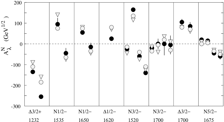
FIG. 21.: Breit-frame photoproduction amplitudes for $\Delta{\textstyle{3\over 2}}^{+}(1232)$ and the $P$-wave resonances, in units of $10^{-3}$ GeV^-1/2. Solid circles with error bars are photocouplings from the data analyses of Ref. [3], triangles are the fit $A_{1}^{M}$ from Li and Close [112], and circles are for the relativized calculations from Ref. [114]. Amplitudes are plotted, from left to right, in the order $A_{1/2}$, $A_{3/2}$ for $\Delta$ states, and $A^{p}_{1/2}$, $A^{p}_{3/2}$, $A^{n}_{1/2}$, and $A^{n}_{3/2}$ for nucleon states.

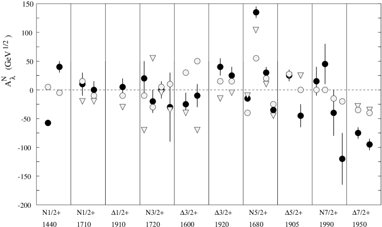
FIG. 22.: Breit-frame photoproduction amplitudes for low-lying (N=2 band) positive-parity excited states for which there exist amplitudes extracted from the data, in units of $10^{-3}$ GeV^-1/2. Caption as in Fig. 21.

The relativized model of Ref. [113, 114] improves the photocouplings of the other radial excitation of the nucleon, $N{\textstyle{1\over 2}}^{+}(1710)$, and those of $\Delta{\textstyle{3\over 2}}^{+}(1600)$, a radial excitation of $\Delta(1232)$, are also somewhat improved (largely by the correct prediction of the sign of the amplitude). The relativized model has slightly more freedom to fit the photocouplings, as the effective quark mass $m^{*}$ in the electromagnetic transition operator is allowed to vary and is fit to the photocouplings, while the quark magnetic moments are held fixed. Close and Li [111, 112] show that $m^{*}$ should be thought of as the sum of the average kinetic and scalar-binding potential energy of the constituent quarks. Neither model is able to account for the small photocoupling of $\Delta{\textstyle{1\over 2}}^{-}(1620)$ or the (relatively precisely determined) large $A^{p}_{3/2}$ amplitude of $N{\textstyle{5\over 2}}^{+}(1680)$ found in the analyses. The next generation of experiments at new facilities such as CEBAF at the Jefferson Laboratory will examine the pion photoproduction and electroproduction processes; the latter will yield the $Q^{2}$ dependence of the Roper resonance EM couplings, for example. It is also obvious that a model of the process $\gamma N\to N\pi$ at 1440 MeV which includes pionic dressing of the vertex is required to understand the Roper resonance EM couplings, since this state couples very strongly to $N\pi$ and as a light state its decay pion is relatively slow moving.

C collective model

Bijker, Iachello and Leviatan (BIL) also calculate photocouplings [87] in their algebraic collective model approach. Their calculation in this model involves writing the transition operator in terms of the constituent coordinates and momenta, transcribing this in terms of the bosonized coordinates and so elements of the algebra, and then algebraically evaluating their matrix elements in the basis. As the charge and magnetic moments of the quarks are viewed in their model as distributed along the Y-shaped string making up the baryon, it is not simple to accomplish the first of these steps. The approach outlined above is to look at the nonrelativistic reduction of the coupling of point-like quarks to the electromagnetic field. However, the resulting form is momentum dependent and so cannot be used in this approach. A transformation is made to coordinate-dependent terms by replacing the quark momenta ${\bf p}_{i}/m_{i}$ by $ik_{0}{\bf r}_{i}$, where $k_{0}$ is the photon energy. The spin-orbit and two-body terms required for a consistent expansion to order $({\bf p}/m)^{2}$ are dropped, and the two terms in the nonrelativistic interaction Hamiltonian in Eq. (59) are then viewed as electric and magnetic contributions. The resulting operator can then be written in terms of the operators which make up the spectrum-generating algebra.

The results of evaluating the photocouplings using this model are also shown in Tables I and II. BIL believe that the sign of the photocouplings (which are inclusive of the sign of the $A_{X\to N\pi}$ strong decay amplitude) cannot be determined by calculations and so are arbitrary. The signs quoted for their amplitudes are therefore to be used only to compare different amplitudes for the same excited baryon. This limits the usefulness of the comparison of their amplitudes with those extracted from the data. Nevertheless, the fit appears degraded relative to the Li and Close (LC) and Capstick (SC) models. Their model also predicts a large $A^{p}_{\textstyle{1\over 2}}$ amplitude for $N{\textstyle{3\over 2}}^{+}(1720)$ which is not seen in the analyses. They are also unable to fit the substantial photocouplings of the Roper resonance (although the mass is fit well); their results for the photocouplings are zero. As their model does not include configuration mixing due to hyperfine tensor interactions, which are important in describing the photocouplings of the P-wave excited baryons, they must introduce a mixing angle of 38^∘ between the $N{\textstyle{1\over 2}}^{+}(1525)$ and $N{\textstyle{1\over 2}}^{+}(1650)$, not calculated in their model, in order to roughly fit the photocouplings of these states.

VI Strong Decay Couplings

A missing states and $N\pi$ couplings

One of the features that many of the models described in the previous sections have in common is that they predict more states than have been experimentally ‘observed’. This would appear to be a problem for such models, as they would clearly have failed to describe physical reality. There are two possible interpretations to this.

A number of authors suggest that the mismatch between the number of baryonic states observed, and the number predicted in some models, is due to the fact that such models are using the wrong degrees of freedom. According to these authors, the three-quark picture of a baryon is flawed, as a baryon in fact consists of a diquark and a quark [83, 84]. The diquark is assumed to be tightly bound, so that the low-lying excitations of the nucleon will not include excitations of the diquark, thus leading to fewer states in the excitation spectrum. The tight binding is thought to occur in the isoscalar scalar channel, due to an attractive hyperfine interaction between a $u$ and a $d$ quark. However, there is some evidence from the lattice [85] and from an analysis of baryon strong decays [86] that such strong diquark clustering may not be present.

A very important consideration here is that of how the experimentally observed states are produced and observed. To date, the vast majority of known excitations of the nucleon have been produced in $\pi N$ elastic scattering, with a few more being ‘observed’ in $\pi N$ inelastic processes like $\pi N\to\pi\pi N$. ‘Observed’ is not completely accurate, however, as all information regarding the baryon spectrum is inferred from fits to the scattering cross sections. Thus, the most precise interpretation of an unobserved state is that such a state is not required to significantly improve the quality of the fit to the available scattering data.

Stated differently, this means that the missing states are ones that do not provide significant contributions to the cross section of the scattering process being examined, namely $N\pi$ elastic scattering, and they must therefore couple weakly to this channel. Faiman and Hendry [47, 120] were among the earliest to suggest this idea in the literature. It is therefore crucial that the observed pattern of $N\pi$ decay widths be reproduced by theoretical treatments, particularly by those models that have a surfeit of states. Furthermore, since the missing states are difficult to detect in the $N\pi$ channel, these models should predict the channels in which they are most likely to be seen. A number of models have treated these strong decays in this manner.

As with their masses, the description of the strong properties of baryons, namely the strong decay widths, coupling constants and form factors, relies largely on phenomenological models, although some work has been done using effective Lagrangians. As few excited states have been treated in the effective Lagrangian approaches, the focus of this section is mainly on the phenomenological approaches.

The operators responsible for strong transitions between baryons arise from non-perturbative QCD, and are therefore essentially unknown. The models that have been constructed assume that the mechanism of the strong decay is either elementary meson emission, quark pair creation, string breaking, or flux-tube breaking. These are illustrated below. The latter three can all be broadly called quark-pair creation models.

The OZI-allowed [121, 122, 123] strong decays of hadrons which are considered here have been examined in three classes of models described below. The ‘hadrodynamic’ models, illustrated in Figure 23, in which all hadrons are treated as elementary point-like objects, do not lend themselves easily to decay calculations of the kind considered here. This is understandable, since each transition is described in terms of one or more independent phenomenological coupling constants, $g_{BB^{\prime}M}$, which means that such models have little predictive power. While the use of SU(2) or SU(3) flavor symmetry arguments give relationships among some of these coupling constants, the overall situation would nevertheless be largely unworkable. It does not appear as if there have been systematic studies of baryon decays using this approach.

FIG. 23.: The process $B\to B^{\prime}M$, as an elementary meson emission from a point-like baryon.

A second class of models treats the baryons as objects with structure, but the decay takes place through elementary meson emission. Such an approach may be taken in bag models, for instance. Some potential model-based calculations, such as the work of Koniuk and Isgur [124, 46], have used a similar approach. In these models, mesons are emitted from quark lines (Figure 24), and the set of $g_{BB^{\prime}M}$ coupling constants is replaced with a smaller set of $g_{qq^{\prime}M}$. In addition, SU(2) or SU(3) flavor symmetry may be used to relate the coupling constants for mesons within a single multiplet, as well as those for different quarks.

FIG. 24.: The process $B\to B^{\prime}M$, as an elementary meson emission from a quark.

Among the earliest descriptions of the strong decays of baryons is the work of Faiman and Hendry (FH) [47, 120]. They assume that the decay occurs through the ‘de-excitation’ of a single quark in the baryon. Their model is thus an elementary meson emission model, and their non-relativistic transition operator takes the form

$${\cal O}=\sum_{j}\frac{f_{q}}{\mu}\left(\mbox{\boldmath$\sigma$}_{j}\cdot\mbox{\boldmath$k$}\right)\left(\mbox{\boldmath$\tau$}_{j}\cdot\mbox{\boldmath$\pi$}\right)e^{i\mbox{\boldmath$k$}\cdot\mbox{\boldmath$r$}_{j}}\left(\frac{1}{2E_{\pi}}\right)^{1/2},$$ (65)

where $\mu$ is taken to be the pion mass, $f_{q}$ is the quark-pion coupling constant, $E_{\pi}$ and $k$ are the energy and momentum of the emitted pion, $\mbox{\boldmath$\sigma$}_{j}$ is the Pauli spin matrix, $\mbox{\boldmath$\tau$}_{j}$ is the isospin operator of the quark from which the pion is emitted, $\mbox{\boldmath$r$}_{j}$ is its position, and the sum over $j$ is over all the quarks in the baryon. This operator was first proposed by Becchi and Morpurgo [125, 126, 127].

In their work, FH find that they are able to reproduce the partial widths available at that time with remarkable accuracy. They propose that the missing resonances simply couple weakly to the $N\pi$ formation channel. They also suggest that the $\Delta\pi$ and other inelastic channels are likely to yield signals for the missing states.

Several authors use a slightly different version of the elementary meson emission model to calculate the decay widths for processes with a pseudoscalar meson in the final state. The elementary meson emission models of Bijker, Iachello and Leviatan (BIL) [128], Koniuk and Isgur (KI) [124, 46], and Sartor and Stancu (SAS) [129] are discussed here. In addition, Koniuk extends this idea to the discussion of vector meson emission [130].

The operator responsible for the emission of a pseudoscalar meson is usually assumed to have the form

$${\cal H_{P}}=\sum_{i=1}^{3}{\cal N}\left(g\mbox{\boldmath$k$}\cdot\mbox{\boldmath$s$}^{(i)}+h\mbox{\boldmath$p$}_{i}\cdot\mbox{\boldmath$s$}^{(i)}\right)e^{-i\mbox{\boldmath$k$}\cdot\mbox{\boldmath$r$}_{i}}X_{i}^{P},$$ (66)

where $k$ is the momentum of the emitted meson, $\mbox{\boldmath$p$}_{i}$ is the momentum of the $i$th quark, $\mbox{\boldmath$r$}_{i}$ is its position, $s$ is its spin, $g$ and $h$ are phenomenological constants, and the $X_{i}^{P}$ are flavor matrices that describe the quark transitions $q_{i}\to q_{i}^{\prime}+P$, where $P$ is a pseudoscalar meson. This is the simplest form that can be written down for this operator. The normalization constant ${\cal N}$ varies with the author, and has the values

$${\cal N} = \frac{1}{(2\pi)^{3/2}(2E_{\pi})^{1/2}},\,\,\,\,\,\,{\rm(BIL)}$$ (67)

$${\cal N} = \frac{i}{(2\pi)^{3/2}},\,\,\,\,\,\,{\rm(KI)}$$ (68)

$${\cal N} = 1.\,\,\,\,\,\,{\rm(SAS)}$$ (69)

In the case of KI and SAS, the symmetry of the wave functions is used to rewrite the transition operator as

$${\cal H_{P}}=3{\cal N}\left(g\mbox{\boldmath$k$}\cdot\mbox{\boldmath$s$}^{(3)}+h\mbox{\boldmath$p$}_{3}\cdot\mbox{\boldmath$s$}^{(3)}\right)e^{-i\mbox{\boldmath$k$}\cdot\mbox{\boldmath$r$}_{3}}X_{3}^{m},$$ (70)

where all the ‘3’ indices refer to the third quark.

The flavor matrices $X^{P}$ are

$$X^{\pi^{0}} = \lambda_{3},\,\,X^{\pi^{+}}=-\frac{1}{\sqrt{2}}\left(\lambda_{1}-i\lambda_{2}\right),X^{\pi^{-}}=\frac{1}{\sqrt{2}}\left(\lambda_{1}+i\lambda_{2}\right),$$ (71)

$$X^{K^{0}} = -\frac{1}{\sqrt{2}}\left(\lambda_{6}-i\lambda_{7}\right),\,\,X^{K^{+}}=-\frac{1}{\sqrt{2}}\left(\lambda_{4}-i\lambda_{5}\right),X^{K^{-}}=\frac{1}{\sqrt{2}}\left(\lambda_{4}+i\lambda_{5}\right),$$ (72)

$$X^{\eta_{1}} = \sqrt{\frac{2}{3}}{\cal I},\,\,X^{\eta_{8}}=\lambda_{8},$$ (73)

where the $\lambda_{i}$ are the Gell-Mann matrices, and ${\cal I}$ denotes the unit operator in flavor space.

The physical $\eta$ and $\eta^{\prime}$ mesons have the flavor compositions

$$\eta=\eta_{8}\cos{\theta}-\eta_{1}\sin{\theta},\,\,\,\eta^{\prime}=\eta_{8}\sin{\theta}+\eta_{1}\cos{\theta},$$ (74)

where

$$\eta_{8}=\frac{1}{\sqrt{6}}\left(u\bar{u}+d\bar{d}-2s\bar{s}\right),\,\,\,\eta_{1}=\frac{1}{\sqrt{3}}\left(u\bar{u}+d\bar{d}+s\bar{s}\right).$$ (75)

For the mixing angles, KI use

$$\eta=\frac{1}{2}\left(u\bar{u}+d\bar{d}-\sqrt{2}s\bar{s}\right),$$ (76)

corresponding to $\theta=-9.7^{\circ}$, while BIL use $\theta=-23^{\circ}$.

A third class of models may be referred to broadly as pair creation models. In such models both the baryons and mesons have structure, and the decay of the baryon, say, occurs by the creation of a quark-antiquark pair somewhere in the hadronic medium. The created antiquark combines with one of the quarks from the decaying baryon to form the daughter meson, while the quark of the created pair becomes part of the daughter baryon. This is illustrated in Figure 25.

There are several types of pair creation model. In the ${}^{3}P_{0}$ model, first formulated by Micu [131] and subsequently popularized by LeYaouanc et al. [132, 133, 134, 135, 136, 137], the quark-antiquark pair is created anywhere in space with the quantum numbers of the QCD vacuum, namely $0^{++}$. This corresponds to the quantum numbers ${}^{2S+1}L_{J}={{}^{3}P_{0}}$, hence the name of the model. While the pair, in principle, may be created very far away from the decaying hadron, the wave function overlaps required naturally suppress such contributions to the decay amplitude. This model has been quite popular in descriptions of hadron decays, and has been applied to baryon decays [132, 133, 134, 135, 136], meson decays [131, 132, 133, 134, 135, 136, 138], and even the decays of fictitious four-quark states [139, 140, 141, 142, 143]. The popularity of this model stems from its overall simplicity, and the fact that, when first proposed, it could be applied to both meson and baryon decays. In addition, it naturally provides the centrifugal barrier to the transition amplitudes needed to describe the strong decays.

Other pair-creation models include the string-breaking models of Dosch and Gromes [144], and of Alcock, Burfitt and Cottingham [145]. In these models, the lines of color flux between quarks have collapsed into a string, and the pair is created when the string breaks. This is illustrated in Figure 26. In the Dosch-Gromes version of this model, the created pair have the quantum numbers ${}^{3}P_{0}$, while in the Alcock et al. version, the quantum numbers of the created pair are ${}^{3}S_{1}$. Note that in all versions of the ${}^{3}S_{1}$ model, the operator is taken to be proportional to the scalar product of the spin of the created quark-antiquark pair, with some vector in coordinate space. Thus, the operator is still a $0^{+}$ operator, which means that many aspects of the ${}^{3}S_{1}$ model are very similar to those of the ${}^{3}P_{0}$ model. Fujiwara [146] also explores the strong decays of the $P$-wave baryons in a ${}^{3}S_{1}$ pair-creation model.

FIG. 25.: The OZI allowed process $B\to B^{\prime}M$, in a quark pair creation scenario.

FIG. 26.: The process $B\to B^{\prime}M$ in the string breaking picture.

Recently, Ackleh, Barnes, and Swanson [147] show that meson strong decays can be described by interactions between the quarks in the parent hadron and the created quark pair which are similar to the interactions used in potential models, namely one-gluon-exchange and confinement. They show that this leads to an effective decay operator which is dominantly ${}^{3}P_{0}$, although sometimes because of quantum numbers the sub-dominant ${}^{3}S_{1}$ form plays a role. Just as importantly, they show that their picture of the decay process yields an effective pair creation strength $\gamma$ close to that used in ${}^{3}P_{0}$ models, when they use parameters similar to those used in potential models.

The transition operator for the ${}^{3}P_{0}$ model is assumed to be

$$T = -3\gamma\sum_{i,j}\int d\mbox{\boldmath$p$}_{i}\/d\mbox{\boldmath$p$}_{j}\/\delta(\mbox{\boldmath$p$}_{i}\/+\mbox{\boldmath$p$}_{j}\/)C_{ij}F_{ij}$$ (77)

$$\times \sum_{m}<1,m;1,-m|0,0>\chi_{ij}^{m}{\cal Y\/}_{1}^{-m}(\mbox{\boldmath$p$}_{i}\/-\mbox{\boldmath$p$}_{j}\/)b_{i}^{\dagger}(\mbox{\boldmath$p$}_{i}\/)d_{j}^{\dagger}(\mbox{\boldmath$p$}_{j}\/).$$ (78)

Here, $C_{ij}$ and $F_{ij}$ are the color and flavor wave functions of the created pair, both assumed to be singlet, $\chi_{ij}$ is the spin triplet wave function of the pair, and ${\cal Y}_{1}(\mbox{\boldmath$p$}_{i}-\mbox{\boldmath$p$}_{j})$ is the vector harmonic indicating that the pair is in a relative $p$-wave.

For the transition $A\to BC$, the transition amplitude $M$ is evaluated, where

$$M_{A\to BC}(k_{0})=<B(k_{0})C(-k_{0})|T|A(0)>,$$ (79)

and a partial decay width is calculated as

$$\Gamma(A\to BC)=\left|M_{A\to BC}(k_{0})\right|^{2}\Phi(ABC),$$ (80)

where $\Phi$ is the phase space for the decay. Details of the calculation of the matrix elements of this operator, or of the operator chosen for elementary meson emission, are omitted here for reasons of compactness. For the phase space factor $\Phi$, a number of options have been used. The usual prescription is

$$\Phi(ABC)=2\pi{E_{B}(k_{0})E_{C}(k_{0})k_{0}\over m_{A}},$$ (81)

with $E_{B}(k_{0})=\sqrt{k^{2}_{0}+m_{B}^{2}}$, $E_{C}(k_{0})=\sqrt{k^{2}_{0}+m_{C}^{2}}$. This is a ‘semi-relativistic’ prescription, since it is usually used with a matrix element calculated non-relativistically, while $E_{B}$ and $E_{C}$ have been calculated relativistically. A fully nonrelativistic prescription consists in using

$$\Phi(ABC)=2\pi{m_{B}m_{C}k_{0}\over m_{A}}.$$ (82)

In their calculation of meson decay widths, Kokoski and Isgur [150] use the prescription

$$\Phi(ABC)=2\pi{\tilde{m}_{B}\tilde{m}_{C}k_{0}\over\tilde{m}_{A}},$$ (83)

where the $\tilde{m}$’s are effective hadron masses, evaluated with a spin-independent inter-quark interaction. They argue that this is valid in the weak-binding limit, where $\rho$ and $\pi$ are degenerate.

In the baryon decay width calculation of Capstick and Roberts (CR) [61, 148, 149], there are some features that are similar to the Kokoski-Isgur calculation of the meson decay widths: (i) the baryon wave functions used [56] are obtained in the same spirit as the Godfrey-Isgur [55] wave functions used in the Kokoski-Isgur calculation, and in fact, many of the parameters of both spectroscopic calculations are chosen to be the same or similar; (ii) the Godfrey-Isgur wave function is used for the pion. CR argue that it makes sense, therefore, to use Eq. (83) in their calculation of the baryon decay widths. For the decays of a resonance $R$ to $N\pi$, they use $\tilde{m}_{N}=1.1$ GeV, $\tilde{m}_{\pi}$=0.72 GeV, consistent with Kokoski and Isgur, and $\tilde{m}_{R}=m_{R}$.

Forsyth and Cutkosky (FC) [51] consider three versions of a pair creation model which, combined with their model for the spectrum, they fit to the Carnegie-Mellon University-Lawrence Berkeley Laboratory partial wave analyses (CMB) [151, 152]. The form that they use for the spatial part of the transition operator is

$${\cal O}=\mbox{\boldmath$S$}\cdot\mbox{\boldmath$V$},$$ (84)

where $S$ is the spin of the created quark-antiquark pair, and $V$ is some vector, chosen to be

$$\mbox{\boldmath$V$}=\left(G_{1}\mbox{\boldmath$p$}_{3}+G_{2}\mbox{\boldmath$p$}^{\prime}_{3}\right)e^{i\mbox{\boldmath$k$}\cdot\mbox{\boldmath$w$}}.$$ (85)

In this expression, $w$ is the separation between the daughter baryon and meson, $\mbox{\boldmath$p$}_{3}$ and $\mbox{\boldmath$p$}_{3}^{\prime}$ are the momenta of the third quark in the parent and daughter baryon, respectively, and $k$ is the momentum of the daughter meson. The form chosen for the operator means that it is a $0^{+}$ operator. This model subsumes many other pair creation models as special cases. As is, this is the model of Horgan [153], while with $G_{1}=-G_{2}$, this becomes the model used by Faiman and Hendry [47, 120]. Setting $G_{1}=0$ results in the ${}^{3}P_{0}$ model as formulated by the Orsay group [132, 133, 134, 135, 136].

The first of the three versions of this model examined by these authors utilizes the full operator, with both $G_{1}$ and $G_{2}$ non-zero. The second is an extension of the model used by KI, in which each distinct polynomial (in $k$) that arises in the evaluation of the spatial matrix elements is replaced by an adjustable parameter. In the third version, $G_{1}$ and $G_{2}$ are allowed to depend on the spin and orbital state of the ‘spectator’ quarks. In this way, they relax the spectator conditions that are usually used in such models. They find that this version of the model works best. However, none of their results are shown here, but the interested reader is referred to the original work.

In selecting the results that are discussed, only those calculations in which a number of decay channels have been treated, for a number of baryon resonance, and for which numbers are easily available, have been chosen. These criteria are applied both to the meson emission and pair creation models. Among the pair-creation models, the work by Le Yaouanc et al. [132, 133, 134, 135, 136, 154] of the Orsay group (OR), CR [61, 148, 149], SST [155, 156, 157, 158, 159, 160, 161, 162], and by Wagenbrunn et al. (WPTV) [80], are discussed and compared with the results obtained in the elementary meson emission models. It must be pointed out here that although only two models for the strong decay processes have been widely used, either one can be combined with the wide range of models for the baryon spectrum, thus leading, in principle, to very diverse predictions for decay widths, coupling constants and form factors.

The results obtained for the $N\pi$ decay widths for the models considered are shown in table III. The first column of the table identifies the state, while columns two to thirteen give the magnitudes of the decay amplitudes into $N\pi$ calculated in the models of OR [132, 133, 134, 135, 136, 154], BIL [128], SAS [129], KI [124, 46, 130], CR [61, 148, 149], (SST) [155, 156, 157, 158, 159, 160, 161, 162] and WPTV [80]. Missing states have their model-predicted masses (here chosen to be those of CR, but other models predict very similar masses) shown in square parentheses. The models of BIL, SAS and KI are elementary meson emission models, while those of OR, CR, SST and WPTV are pair creation models. The numbers obtained from the partial wave analyses [163] are shown in the final column.

For all of the models chosen, the results reported are obtained by first fitting any unknown coupling constants ($g$ and $h$ of Eq. (66) or $\gamma$ of Eq. (77)) to a set of measured widths. SST explore three different scenarios in their article, but results from only two of them are presented. In one of these scenarios, they present results for emission of a point-like pion (the column labeled ‘Point’), while in the other, the pion has a finite size (the column labeled ‘Size’). For each scenario, they fit $\gamma$ to the width of the $\Delta(1232)$.

The numbers obtained by OR result from a fit in which all of the amplitudes that they calculate are included. These amplitudes include not just the $N\pi$ amplitudes of Table III, but also amplitudes into the channels $\Delta\pi$ and $N\rho$. In each channel, numbers for the decays of the $N{\textstyle{1\over 2}}^{+}(1440)$ are not presented, as this resonance has been specially treated by these authors.

For SAS, four numbers are shown, corresponding to four different scenarios in their model. The numbers from Set I result from a particular choice for two parameters that determine their hyperfine and tensor interactions, while Set II results from a different choice for these parameters. Furthermore, they examine the effects of configuration mixing in their wave functions, and for each of Set I and Set II, the column labeled U results from using unmixed wave functions, while the column labeled M results from using mixed wave functions. These authors apparently fit to the $N\pi$ widths of eighteen low-lying resonances (of which all but two are three- and four-star states). Neither SAS nor SST provide $N\pi$ amplitudes for any possible missing states.

The model of BIL involves a third parameter that arises from their description of the distributions (of charge, magnetic moments, etc.) within a baryon, and these three parameters are fit to the widths of all three- and four-star resonances, with the exception of the $S_{11}$ resonances. The results obtained in this model also depend on the quantities $\chi_{1}$ and $\chi_{2}$, which are related to the matrix elements for the vibrational excitations in this collective model. The expressions for $\chi_{1}$ and $\chi_{2}$ are

$$\chi_{1}=\frac{1-R^{2}}{R\sqrt{N}},\,\,\,\chi_{2}=\frac{\sqrt{1+R^{2}}}{R\sqrt{N}},$$ (86)

where $R$ is a size parameter, and $N$ determines the size of the model space used in the calculation. The values of neither $N$ nor $R$ are provided in their articles. However, it appears that the numbers that they present are obtained in the limit $N\to\infty$. In this case, the radial excitations, such as the $N{\textstyle{1\over 2}}^{+}(1440)$, do not decay to the ground state, and the appropriate entries in the tables should be zeroes, instead of quantities that depend on $\chi_{1}$ and $\chi_{2}$.

KI do not explicitly calculate all of their amplitudes using Eq. (66). Instead, they identify four general amplitudes, one of which they term ‘structure independent’, and three that are ‘structure dependent’. They fit these four amplitudes to the numbers obtained from the partial wave analyses, but it is not clear which of the experimental amplitudes are included in their fit.

CR fit to the $N\pi$ widths of all two-, three- and four-star resonances that lie in the $N\leq 2$ oscillator-type bands. All of their numbers show ‘theoretical’ uncertainties. These are obtained from the kinematic dependences of the amplitudes, which are due to the uncertainties in the masses of the states. For an observed state, the quoted decay amplitude is obtained by carrying out the calculation at the centrally reported mass of the state, and the uncertainty on the amplitude is obtained by evaluating the amplitude at the upper and lower limits given by the errors on the mass. For missing or unobserved states, the quoted decay amplitude is obtained using the theoretically predicted mass, while the errors on the amplitude are obtained assuming an error of 150 MeV in the mass of the state.

The wave functions used by WPTV are obtained using one version of the GBE model, and they use the ${}^{3}P_{0}$ operator to calculate the decay amplitudes. They examine a number of scenarios for the $N\pi$ decays. In the column labeled NR, the Hamiltonian used is nonrelativistic, while for the column labeled SR, the kinetic energy operator for the quarks is the relativistic one. In both cases, these authors fit to the amplitude for the decay $\Delta\to N\pi$. They also explore the role of the pion size, and present results for two different pion radii. However, results for a single pion size are presented here. It may be noted that an extended pion appears to be inconsistent with one of the basic tenets of the GBE model, namely that the pion is a special, structure-less object that gives rise to the potential between the quarks.

It is difficult to assess the efficacy of these models by simply examining the rows of numbers presented. In the last four rows of Table III, the $\chi^{2}$ values for each of the models is presented. This quantity is evaluated as

$$\chi^{2}=\frac{1}{n}\sum_{i}^{n}\frac{\left(T_{i}-E_{i}\right)^{2}}{\sigma_{i}^{2}},$$ (87)

where $T_{i}$ is the model prediction for the amplitude, $E_{i}$ is the amplitude extracted from the partial wave analyses, $\sigma_{i}$ is the uncertainty of the extracted amplitude, and the sum includes all states for which a particular model makes a prediction. A second measure of the efficacy of each model, is the theoretical error $\tau$, defined by the expression

$$n=\sum_{i}^{n}\frac{\left(T_{i}-E_{i}\right)^{2}}{\sigma_{i}^{2}+\tau^{2}}.$$ (88)

Two values each of $\chi^{2}$ and $\tau$ are presented. In the first set of numbers, all calculated amplitudes for which there are experimental analogs are used. In the second set of numbers, the state $N{\textstyle{3\over 2}}^{+}(1720)$ is omitted, as a number of models predict very large values for its amplitude into the $N\pi$ channel.

TABLE III.: $N\pi$ decay widths for the models considered here. The first column identifies the state, while columns two to thirteen give the magnitude of the decay amplitudes into $N\pi$ calculated in the models of OR [132, 133, 134, 135, 136], BIL [128], SAS [129], KI [46, 124], CR [61], SST [155, 156, 157, 158, 161, 162] and WPTV [80], respectively. The numbers obtained from the partial wave analyses [163] are shown in column 14, labeled PWA. Missing states have their masses shown in square parentheses. The models of BIL, SAS and KI are elementary meson emission models, while those of OR, CR, SST and WPTV are pair creation models. For SAS, four numbers are shown, corresponding to four different scenarios in their model. Two numbers are shown for each of the SST and WPTV models. For BIL, the quantities $\chi_{1}$ and $\chi_{2}$ are defined in the text. The last four rows show the average $\chi^{2}$ per amplitude (calculated using only observed states), as well as the theoretical error, defined in the text, for each of the models.

state	OR	BIL	SAS				KI	CR	SST		WPTV		PWA
			Set I		Set II
			U	M	U	M			Point	Size	NR	SR
$N{\textstyle{1\over 2}}^{-}(1535)$	3.8	9.2	20.3	14.9	14.3	9.4	5.3	$14.4\pm 0.7$	18.3	12.9	11.8	6.3	8.0$\pm$2.8
$N{\textstyle{1\over 2}}^{-}(1650)$	5.1	5.9	8.7	12.7	6.0	8.9	8.7	$10.7\pm 1.1$	19.6	2.3	4.0	7.4	8.7$\pm$1.9
$N{\textstyle{3\over 2}}^{-}(1520)$	6.0	10.7	8.4	8.5	5.0	5.0	9.2	$10.0\pm 0.3$	4.5	8.4	15.1	6.7	8.3$\pm$0.9
$N{\textstyle{3\over 2}}^{-}(1700)$	1.9	2.2	2.3	3.4	1.5	2.3	3.6	$6.0\pm 0.4$	2.3	4.1	2.0	1.0	3.2$\pm$1.3
$N{\textstyle{5\over 2}}^{-}(1675)$	4.1	5.6	5.0	5.2	3.1	3.4	5.5	$5.7\pm 0.1$	3.1	5.6	4.8	2.0	7.7$\pm$0.7
$N{\textstyle{1\over 2}}^{+}(1440)$	8.9	10.4$\chi_{1}$	0.3	0.1	1.2	1.0	6.8	$22.2^{+0.6}_{-0.4}$	4.9	20.8	16.2	23.0	19.7$\pm$3.2
$N{\textstyle{1\over 2}}^{+}(1710)$	5.1	13.2$\chi_{2}$	1.4	9.1	0.1	6.0	6.7	$3.4\pm 0.3$	3.5	1.8	4.0	7.4	4.7$\pm$1.2
$N{\textstyle{1\over 2}}^{+}[1880]$		4.7					4.4	$3.0^{+1.1}_{-1.3}$
$N{\textstyle{1\over 2}}^{+}[1975]$		1.3					1.2	$1.6^{+0.6}_{-0.5}$
$N{\textstyle{3\over 2}}^{+}(1720)$	8.5	5.6	0.4	10.8	0.1	8.6	6.5	$17.1^{+0.5}_{-0.4}$	16.9	7.1	10.4	19.2	5.5$\pm$1.6
$N{\textstyle{3\over 2}}^{+}[1870]$		1.5					3.2	$5.6^{+1.9}_{-1.6}$
$N{\textstyle{3\over 2}}^{+}[1910]$		8.1					1.1	$0.2\pm 0.4$
$N{\textstyle{3\over 2}}^{+}[1950]$		8.4					1.1	$4.2^{+1.2}_{-1.1}$
$N{\textstyle{3\over 2}}^{+}[2030]$		3.9					0.5	$1.9^{+0.5}_{-0.4}$
$N{\textstyle{5\over 2}}^{+}(1680)$	6.0	6.4	7.6	7.9	3.9	3.6	7.1	$9.3\pm 0.2$	3.2	9.7	9.4	8.9	8.7$\pm$0.9
$N{\textstyle{5\over 2}}^{+}[1980]$		8.2					0.4	$1.0\pm 0.1$
$N{\textstyle{5\over 2}}^{+}(2000)$							1.3	$1.3\pm 0.2$	0.7	2.0			2.0$\pm$1.2
$N{\textstyle{7\over 2}}^{+}(1990)$							3.1	$3.0\pm 0.3$	0.6	1.8			$4.6\pm 1.9$
$\Delta{\textstyle{1\over 2}}^{-}(1620)$	2.4	4.0	6.3	5.8	4.2	3.7	3.3	$4.6\pm 0.9$	8.3	0.6	2.5	2.0	$6.5\pm 1.0$
$\Delta{\textstyle{3\over 2}}^{-}(1700)$	3.8	5.2	4.1	4.3	2.7	2.9	4.9	$5.2\pm 0.5$	2.7	4.8	4.0	1.8	$6.5\pm 2.0$
$\Delta{\textstyle{1\over 2}}^{+}(1740)^{a}$							2.7	$3.9^{+0.4}_{-0.7}$					$4.9\pm 1.3$
$\Delta{\textstyle{1\over 2}}^{+}(1910)$	5.7	6.5	0.9	6.1	0.4	6.4	5.3	$9.9^{+0.7}_{-0.8}$	7.8	0.7			$6.6\pm 1.6$
$\Delta{\textstyle{3\over 2}}^{+}(1232)$		10.8	10.0	10.5	10.5	10.9	11.0	$10.2\pm 0.1$	10.7	10.7	11.0	11.0	$10.7\pm 0.3$
$\Delta{\textstyle{3\over 2}}^{+}(1600)$	19.0	10.4$\chi_{1}$	2.8	14.0	1.8	10.6	5.4	$6.3^{+1.9}_{-1.6}$	9.0	0.2	6.3	6.7	$7.6\pm 2.3$
$\Delta{\textstyle{3\over 2}}^{+}(1920)$		4.7	4.0	0.7	3.4	4.1	5.2	$4.6\pm 0.5$	1.7	2.0			$7.7\pm 2.3$
$\Delta{\textstyle{3\over 2}}^{+}[1985]$							0.1	$3.7^{+1.4}_{-1.5}$
$\Delta{\textstyle{5\over 2}}^{+}(1750)$								$2.0\pm 0.8$
$\Delta{\textstyle{5\over 2}}^{+}(1905)$	3.8	3.0	3.4	2.7	2.0	1.1	4.0	$4.3^{+0.2}_{-0.3}$	1.2	3.1			$5.5\pm 2.7$
$\Delta{\textstyle{5\over 2}}^{+}(2000)$							1.0	$1.3^{+0.2}_{-0.3}$					$5.3\pm 2.3$
$\Delta{\textstyle{7\over 2}}^{+}(1950)$	9.8	6.7	7.1	6.2	4.2	3.6	7.5	$8.5\pm 0.1$	3.9	8.7			$9.8\pm 2.7$
$\chi^{2}_{a}$	7.2	3.5 (5.9)	7.0	6.4	11.4	8.6	2.7	4.6	12.9	5.3	8.7	13.8
$\tau_{a}$	4.1	2.2 (4.8)	5.5	5.3	5.6	4.8	2.2	2.9	5.9	3.1	3.1	4.5
$\chi^{2}_{b}$	7.4	3.8 (6.3)	6.8	6.1	11.4	8.9	2.9	2.2	10.8	5.5	8.7	8.9
$\tau_{b}$	4.2	2.3 (5.0)	5.6	5.3	5.6	4.9	2.3	1.4	5.4	3.2	2.9	2.6

^a First $P_{31}$ state found in Ref. [48].

At first glance, all of the models seem to describe the amplitudes with similar kinds of success. However, examination of the $\chi^{2}$ values, as well as the $\tau$ values, gives some indication that a few of the models do better at describing the decays. For BIL, the amplitudes for the radial excitations $N{\textstyle{1\over 2}}^{+}(1440)$, $N{\textstyle{1\over 2}}^{+}(1710)$ and $\Delta{\textstyle{3\over 2}}^{+}(1600)$ depend on two quantities, $\chi_{1}$ and $\chi_{2}$, which in turn depend on $R$ and $N$. Here, $N$ is determined by the size of the model space that they use in obtaining the spectrum. In a more recent article [89], these authors treat $\chi_{1}$ and $\chi_{2}$ as constants with values of 1.0 and 0.7, respectively, values that are inconsistent with the large $N$ limit. The corresponding widths that they report are $N\pi$ widths of 108 MeV, 85 MeV and 108 MeV, respectively, for the three states in question. When these widths are used in the calculation of $\chi^{2}$ and $\tau$, the values obtained are as shown in the table. However, all the rest of the BIL results appear to be obtained in the limit of $N\to\infty$, which means that these three amplitudes are zero. Using these vanishing amplitudes leads to the values of $\chi^{2}$ and $\tau$ shown in parentheses in the table.

It must be emphasized that the values of $\chi^{2}$ and $\tau$ are to be interpreted with care, as they depend very strongly on which states are included in the calculation, as well as on the values taken for the extracted amplitudes. For instance, if the $N\pi$ amplitude for the $N{\textstyle{1\over 2}}^{+}(1440)$ from Ref. [163] is used, then the quality of the models by CR, SST and WPTV would certainly appear to deteriorate, while all of the elementary emission models would improve. Similarly, if the amplitudes for less-well-known resonances are omitted from the calculation, some models would again improve, and others deteriorate. In addition, it must be pointed out that the model of OR appears to do poorly when compared with many of the others, but their $N\pi$ amplitudes were fit to the partial wave analyses available more than twenty-five years ago, and many of those numbers have changed. Furthermore, they fit not only $N\pi$ amplitudes, but $\Delta\pi$ and $N\rho$ as well. Thus, the quality of their $N\pi$ predictions has suffered.

There are significant disagreements among the model predictions for the $N\pi$ amplitudes of these low-lying states, and these differences become more apparent when other decay channels are included in the comparison. One of the more striking disagreements among the models is the prediction of SAS for the decay of the Roper resonance. Their results disagree with all the other models, and with the results obtained from the partial wave analyses.

The role of the kinetic energy of the quarks is seen in the comparison of the two sets of numbers obtained from the model of WPTV. In fact, changing the kinetic energy operator in the Hamiltonian from the nonrelativistic to the semi-relativistic has resulted in differences of factors of two in some of the $N\pi$ amplitudes.

The effects of configuration mixing are clearly seen in the decay widths that result from the different scenarios explored by SAS. The calculated decay widths of the $S_{11}$ resonances, as well as those of the $P_{11}$, $P_{13}$, $P_{31}$ and $P_{33}$ resonances, are very different depending on whether the wave functions used include the effects of mixing or not. Note, too, that the OR and CR decay models are very similar, but the OR wave functions have no configuration mixing, while those of the CR model do. This difference accounts for much of the differences between the two sets of predictions, which are often different by more than a factor of two. These differences also make it clear that predictions for the spectrum of states produced in a particular model are not very sensitive probes of the wave functions. All of the wave functions used in these calculations have been obtained from fits to the spectrum of states that are of similar quality, yet the predictions for the strong decay widths are very different.

Another striking effect illustrated in this table is that of using a point-like pion in describing the decays. This is seen in comparing the two sets of numbers taken from the model of SST. This effect is seen most strongly in the numbers predicted for the $S_{11}$ resonances, as well as those of the $P_{11}$, $P_{13}$, $P_{31}$ and $P_{33}$ resonances, just as with configuration mixing. A more striking illustration of this is the fact that almost all the meson emission models predict very small amplitudes for the $N\pi$ decay of the $P_{11}(1440)$, while the pair-creation models predict large amplitudes for these decays. KI predict a relatively large amplitude for this decay, but one must keep in mind that these authors did not calculate the decay amplitudes, but fit sets of amplitudes.

Perhaps the state most sensitive to the scenarios explored by the different authors is the Roper resonance, $N{\textstyle{1\over 2}}^{+}(1440)$. For point-like pions, most authors obtain very small $N\pi$ decay widths for this state (with the exception of KI, as pointed out in the previous paragraph). For pions with structure, the predicted partial widths are very large, very much in agreement with the partial wave analysis of Cutkosky and Wang [103]. It must be pointed out, however, that many partial wave analyses give values of the order of 100 to 150 MeV for this partial width, values that would appear difficult to accommodate in most of the models discussed in Table III.

This state has been responsible for generating many articles on its nature, its mass, and most recently, on the origin of the interquark potential in potential models. Recently, for instance, Li, Burkert and Li [94], as well as Kisslinger and Li [95], suggest that this state might not be one of the usual $qqq$ states, but a hybrid, instead. SST also attempt to improve their description of this resonance by modifying the main component of its radial wave function [62]. In so doing, they are able to lower its mass by about 100 MeV. Other authors, most recently Krehl et al. [104], suggest that this resonance can be interpreted in terms of meson-baryon dynamics alone, with no need for a three-quark resonance. Finally, it should be noted that the recent spate of GBE models described in previous sections originate in part to explain the somewhat low mass of this state, as models relying on one-gluon exchange in the potential usually place this state about 100 MeV heavier. Whatever the nature of this state, it is clear that more precise scattering data, as well as more rigorous analyses of these scattering data, are needed to shed some light on these questions.

To a large extent, the models examined above predict relatively small $N\pi$ widths for the missing baryons. Again, however, there are exceptions, and these come mainly from the model by BIL. Table III does not show all of the missing states that they predict [89]. As pointed out in an earlier section, this model predicts at least fourteen missing nucleon resonances below 2 GeV, more than any other model. In addition, six of these resonances have appreciable couplings to the $N\pi$ formation channel, with four of them having $N\pi$ partial widths greater than 50 MeV. In contrast with this, four of their light missing states do not couple to any of the channels ($N\pi$, $\Delta\pi$, $N\eta$, $\Sigma K$, $\Lambda K$, $\Sigma^{*}K$) investigated by these authors. Some of the $N\pi$ large widths for missing states are probably due to the absence of configuration mixing in their wave functions or to the fact that they use a point-like pion. In fact, these predictions are expected to change if these effects are included in this calculation. Nevertheless, the predictions from this model appear to be difficult to reconcile with existing analyses.

B other channels

With the qualified success of most of these models in explaining the missing states (those that treat missing states), attention can now be turned to the question of where can these missing states be seen. In these models, a number of other channels have been explored, including $N\eta$ and $\Delta\eta$, $\Delta\pi$, $N\rho$ and $N\omega$, as well as some channels containing strange mesons and baryons, such as $\Lambda\bar{K}$ and $\Sigma\bar{K}$. Such calculations not only test the models (by comparing their result with whatever data are available), but also allow predictions of which channels are good candidates for ‘resonance hunting’. In particular, isospin-selective channels like $\Delta\eta$, $N\eta$ and $N\omega$, are quite interesting, as the partial-wave analyses required are expected to be simpler than for some of the other channels, where both $N^{*}$ and $\Delta^{*}$ states are expected to contribute.

In the pair creation models, the treatment of decays involving vector mesons proceeds much as treatment of decays involving pseudoscalar mesons. For elementary vector-meson emission, Koniuk modifies a non-relativistic form that has been used for photon emission, and obtains [130]

$${\cal H}_{V}=-\frac{3i}{(2\pi)^{3/2}}\left[g\left(\mbox{\boldmath$\varepsilon$}^{*}\cdot\mbox{\boldmath$p$}_{3}^{\prime}-\mbox{\boldmath$\varepsilon$}^{*}\cdot\mbox{\boldmath$k$}^{\prime}\frac{E_{3}^{\prime}}{E_{v}}\right)+h\mbox{\boldmath$s$}_{i}\cdot\mbox{\boldmath$k$}\times\mbox{\boldmath$\varepsilon$}^{*}\right]X_{3}^{V}.$$ (89)

Here $\mbox{\boldmath$\varepsilon$}^{*}(\mbox{\boldmath$k$},\lambda)$ is the vector-meson polarization vector, and $X_{3}^{V}$ are flavor matrices that describe the quark transitions $q_{3}\to q_{3}^{\prime}+V$. In this sector, $\phi-\omega$ mixing can be treated in a manner analogous to $\eta-\eta^{\prime}$ mixing, as discussed above. With

$$\omega=V_{8}\cos{\theta}-V_{1}\sin{\theta},\,\,\,\phi=V_{8}\sin{\theta}+V_{1}\cos{\theta},$$ (90)

where $V_{1,8}$ denotes the singlet or octet component of the isoscalar vector meson, and a value of $\theta=54.7^{\circ}$ results if the hidden strangeness component of the $\omega$ vanishes. Note that if

$$g=h=\frac{e}{2m_{3}}\left(\lambda_{3}+\sqrt{\frac{1}{3}}\lambda_{8}\right),$$ (91)

the vector meson emission operator above becomes the lowest order operator for photon emission in a non-relativistic expansion. In this expression, $\lambda_{3}$ and $\lambda_{8}$ are flavor matrices.

For the $N\rho$ and $\Delta\pi$ channels, as well as for $\Delta\eta$, one of the daughter hadrons produced in the decay is a broad one. BIL ignore this, and treat both daughter hadrons in the narrow-width approximation. CR and SST take the width of the daughter hadron into account by writing the width of the quasi-two-body decay $A\to(X_{1}X_{2})_{B}C$ (where $X_{1}$ and $X_{2}$ are the decay products of the hadron $B$) as

$$\Gamma=\int_{0}^{k_{\max}}dk\frac{k^{2}\left|M(k)\right|^{2}\Gamma_{t}(k)}{\left(M_{a}-E_{b}(k)-E_{c}(k)\right)^{2}+\frac{\Gamma_{t}(k)^{2}}{4}},$$ (92)

where $\Gamma_{t}(k)$ is the energy-dependent total width of the unstable daughter hadron, $B$ in this case.

At this point it is necessary to point out some differences in the way KI treat the pseudoscalar emission decays, and the way Koniuk treats the vector emission decays. For each calculation, the coupling constants $g$ and $h$ of Eq. (89) are fit to available partial widths, but it is not clear which partial widths are used in the fit. In treating the $N\rho$ decays, Koniuk integrates over the line-shape of the $\rho$ meson, but the form used for the integral is not given. In contrast, when KI treat the $\Delta\pi$ decays, similar integrals over the line-shape of the $\Delta$ are not carried out.

For the $N\eta$ channel (table IV), results are available from the models of BIL, KI, CR and WPTV, while only BIL and CR consider $\Delta\eta$ (table V). BIL are unable to reproduce the large couplings of the lowest lying $S_{11}$ state to the $N\eta$ channel. This may be due to the fact that their wave functions do not include any configuration mixing from the tensor hyperfine interaction. The fact that they use point-like mesons may also play a role in suppressing this decay in their model. A few other significant disagreements also appear in the $\Delta\eta$ and $\Delta\pi$ channels. In contrast, the models of CR and KI are generally in better agreement. No partial wave analyses have yet been performed on the $\Delta\eta$ channel, but this channel offers the possibility of discovering some of the missing baryon resonances. This is particularly so for the higher lying resonances (not shown in the table), where the available phase space is not a limitation on whether or not the decay can proceed.

In obtaining their results for the $N\eta$ channel, WPTV refit the value of the ${}^{3}P_{0}$ coupling constant in order to match the $N\eta$ decay width of the lowest lying $S_{11}$ resonance. For both scenarios that they explore, this leads to a significant change in the coupling constant. In comparison, BIL, KI and CR use the same value of this coupling constant that they obtain from consideration of the $N\pi$ decays. In Table IV, the results from two different scenarios explored by WPTV are presented. In addition, the results that would have been obtained if the coupling constant were not rescaled are also presented in parentheses. As is apparent from the table, the effect of rescaling is a very significant one.

It should be noted that except for BIL, the other models discussed present signs for the amplitudes of the decays to channels other than $N\pi$. These signs must be understood as being the product of the calculated sign for the $N\pi$ channel, with the calculated sign of the channel being discussed, $N\eta$, say, both calculated in the particular model. This is because the signs of the $N\pi$ amplitudes are inaccessible in an elastic scattering experiment, but the product of the signs of the $N\pi$ and $N\eta$ decay amplitudes are accessible in an inelastic scattering experiment. The signs of the amplitude provide a further means of testing the validity and success of these models. BIL state that all of these signs are arbitrary, and therefore do not present them.

TABLE IV.: $N\eta$ amplitudes for low-lying $N^{*}$ resonances, from the models of BIL [128], CR [148], KI [46, 124] and WPTV [80]. The few experimental data available are shown in the last column.

state	BIL	KI	CR	WPTV		PWA
				NR	SR
$N{\textstyle{1\over 2}}^{-}(1535)$	0.3	+5.2	$+14.6^{+0.7}_{-1.3}$	(22.5) 8.0	(12.1) 8.0	$+8.1\pm 0.8$
$N{\textstyle{1\over 2}}^{-}(1650)$	2.8	-1.5	$-7.8^{+0.1}_{-0.0}$	(18.6) 6.6	(10.1) 6.7	$-2.4\pm 1.6$
$N{\textstyle{3\over 2}}^{-}(1520)$	0.8	+0.4	$+0.4^{+2.9}_{-0.4}$	(0.0) 0.0	(3.9) 2.6
$N{\textstyle{3\over 2}}^{-}(1700)$	2.0	-0.7	$-0.2\pm 0.1$
$N{\textstyle{5\over 2}}^{-}(1675)$	4.1	-2.8	$-2.5\pm 0.2$	(2.8) 1.0	(1.5) 1.0
$N{\textstyle{1\over 2}}^{+}(1440)$			$+0.0^{+1.0}_{-0.0}$
$N{\textstyle{1\over 2}}^{+}(1710)$	4.1 $\chi_{2}$	+2.9	$+5.7\pm 0.3$	(3.9) 1.4	(13.6) 8.9
$N{\textstyle{1\over 2}}^{+}[1880]$		-0.8	$-3.7^{+0.5}_{-0.0}$
$N{\textstyle{1\over 2}}^{+}[1975]$			$+0.1^{+0.2}_{-0.1}$
$N{\textstyle{3\over 2}}^{+}(1720)$	0.5	+1.9	$+5.7\pm 0.3$	(7.3) 2.6	(9.7) 6.4
$N{\textstyle{3\over 2}}^{+}[1870]$		-2.9	$-4.6\pm 0.3$
$N{\textstyle{3\over 2}}^{+}[1910]$			$-0.9\pm 0.1$
$N{\textstyle{3\over 2}}^{+}[1950]$			0.0
$N{\textstyle{3\over 2}}^{+}[2030]$			$+0.4\pm 0.1$
$N{\textstyle{5\over 2}}^{+}(1680)$	0.7	+0.7	$+0.6\pm 0.1$	(2.8) 1.0	(1.5) 1.0
$N{\textstyle{5\over 2}}^{+}[1980]$			$-0.8\pm 0.2$
$N{\textstyle{5\over 2}}^{+}(2000)$		-0.6	$+1.9\pm 0.8$
$N{\textstyle{7\over 2}}^{+}(1990)$		-2.3	$-2.2^{+0.6}_{-0.7}$

TABLE V.: Results for the lowest-lying $\Delta$ states in the $\Delta\eta$ channel. Results from the model calculations of CR [149] and BIL [128] are shown, with results from the different models presented on different rows. Light states with zero amplitudes are omitted from the table.

state	Model	$\Delta\eta$	$\Delta\eta$	$\sqrt{\Gamma^{\rm tot}_{\Delta\eta}}$
		$s$	$d$
$\Delta{\textstyle{3\over 2}}^{-}(1700)$	CR	1.1 ${}^{+3.2}_{-1.1}$	0.0 ${}^{+0.3}_{-0.0}$	1.1 ${}^{+3.2}_{-1.1}$
		$p$
$\Delta{\textstyle{1\over 2}}^{+}(1740)$a	CR	3.2 ${}^{+4.1}_{-3.1}$		3.2 ${}^{+4.1}_{-3.1}$
$\Delta{\textstyle{1\over 2}}^{+}(1910)$	CR	-2.9 $\pm$ 0.7		2.9 $\pm$ 0.7
	BIL			0.0
		$p$	$f$
$\Delta{\textstyle{3\over 2}}^{+}(1600)$	CR	0.0 ${}^{+0.3}_{-0.0}$	0.0 $\pm$ 0.0	0.0 ${}^{+0.3}_{-0.0}$
$\Delta{\textstyle{3\over 2}}^{+}(1920)$	CR	-3.3 $\pm$ 0.9	0.7 $\pm$ 0.4	3.4 $\pm$ 0.9
	BIL			0.7
$\Delta{\textstyle{3\over 2}}^{+}[1985]$	CR	-4.2 ${}^{+2.4}_{-1.7}$	- 0.7 ${}^{+0.6}_{-1.2}$	4.3 ${}^{+1.9}_{-2.5}$
		$p$	$f$
$\Delta{\textstyle{5\over 2}}^{+}(1905)$	CR	-0.5 $\pm$ 0.1	0.6 $\pm$ 0.3	0.8 $\pm$ 0.3
	BIL			1.0
$\Delta{\textstyle{5\over 2}}^{+}(2000)$	CR	-7.0 ${}^{+5.1}_{-2.9}$	0.3 ${}^{+0.8}_{-0.3}$	7.0 ${}^{+2.9}_{-5.1}$
		$f$	$h$
$\Delta{\textstyle{7\over 2}}^{+}(1950)$	CR	0.9 $\pm$ 0.1	0.0 $\pm$ 0.0	0.9 $\pm$ 0.1
	BIL			1.4

^a First $P_{31}$ state found in Ref. [48].

For these channels, no authors have compared results with pointlike and extended daughter mesons, nor with and without configuration mixing. Given the results obtained in the $N\pi$ channel, it is to be expected that the predictions for the quasi-two-body final states will be significantly impacted by the inclusion or exclusion of these two effects. This will certainly influence which channels are good candidates for seeking particular missing baryonic resonances.

The results obtained for the $N\rho$ and $\Delta\pi$ channels are presented in tables VI (for nucleons) and VII (for $\Delta$s), and results there are from CR, BIL, KI, SST and OR ($\Delta\pi$), and from CR, KI, SST and OR ($N\rho$).

TABLE VI.: Results for the lowest-lying nucleons in the $\Delta\pi$, and $N\rho$ channels, for the models by CR [148], KI [46, 124, 130], SST [155, 156, 157, 158, 159, 160, 161, 162], BIL [128] and OR [132, 133, 134, 135, 136]. The results from the different models are on different rows. Also shown are the results from the partial wave analyses (PWA).

state	Model	$\Delta\pi$	$\Delta\pi$	$\sqrt{\Gamma^{\rm tot}_{\Delta\pi}}$	$N\rho$	$N\rho$	$N\rho$	$\sqrt{\Gamma^{\rm tot}_{N\rho}}$
		$d$			$s_{\textstyle{1\over 2}}$	$d_{\textstyle{3\over 2}}$
$N{\textstyle{1\over 2}}^{-}(1535)$	CR	$+1.4\pm 0.3$		$1.4\pm 0.3$	$-0.7\pm 0.1$	$+0.4\pm 0.1$		$0.8^{+0.2}_{-0.1}$
	KI	-1.7		1.7	+6.1	-1.6		6.3
	SST	-4.0		4.0				1.1
	BIL	4.8		4.8
	OR	+0.9		0.9
	PWA	$0.0$		$0.0$	$-1.7\pm 0.6$	$-1.4\pm 0.7$		$2.2\pm 0.6$
$N{\textstyle{1\over 2}}^{-}(1650)$	CR	$+3.6^{+0.8}_{-0.6}$		$3.6^{+0.8}_{-0.6}$	$+0.9^{+0.3}_{-0.2}$	$+0.4\pm 0.1$		$1.0^{+0.3}_{-0.2}$
	KI	-8.2		8.2	+9.7	-2.7		10.1
	SST	-2.6		2.6				0.6
	BIL	4.9		4.9
	OR	-6.2		6.2
	PWA	$+1.7\pm 0.6$		$1.7\pm 0.6$	$0.0$	$+2.2\pm 0.9$		$2.2\pm 0.9$
		$s$	$d$		$d_{\textstyle{1\over 2}}$	$s_{\textstyle{3\over 2}}$	$d_{\textstyle{3\over 2}}$
$N{\textstyle{3\over 2}}^{-}(1520)$	CR	$-5.7^{+3.6}_{-1.6}$	$-1.5^{+1.3}_{-3.0}$	$5.9^{+2.6}_{-3.8}$	$-0.1^{+0.1}_{-0.3}$	$-2.4^{+1.9}_{-6.4}$	$-0.3^{+0.2}_{-1.0}$	$2.5^{+6.5}_{-1.9}$
	KI	+6.7	+2.5	7.2	-0.7	+5.0	+1.1	5.2
	SST	-3.4	+4.4	5.6	+3.2	-1.7	-2.7	4.6
	BIL	1.7	3.0	3.5
	OR	+7.3	+1.3	7.4
	PWA	$-2.6\pm 0.8$	$-4.2\pm 0.6$	$5.0\pm 0.6$		$-5.1\pm 0.6$		$5.1\pm 0.6$
$N{\textstyle{3\over 2}}^{-}(1700)$	CR	$-27.5\pm 1.6$	$+4.6^{+1.6}_{-1.3}$	$27.9^{+1.9}_{-1.8}$	$0.0$	$\pm 0.1\pm 0.0$	$-0.9^{+0.3}_{-0.6}$	$0.9^{+0.6}_{-0.4}$
	KI	+16.0	-7.7	17.8	+0.1	+4.3	+2.7	5.1
	SST	0.5	0.4	0.6				3.7
	BIL	10.5	10.7	15.0
	OR	+13.3	-5.1	14.2
	PWA	$+3.5\pm 3.6$	$+14.1\pm 5.6$	$14.5\pm 5.5$		$-5.6\pm 5.7$		$5.6\pm 5.7$
		$d$	$g$		$d_{\textstyle{1\over 2}}$	$d_{\textstyle{3\over 2}}$	$g_{\textstyle{3\over 2}}$
$N{\textstyle{5\over 2}}^{-}(1675)$	CR	$+5.7\pm 0.4$	$0.0$	$5.7\pm 0.4$	$+0.2\pm 0.0$	$-0.4\pm 0.0$	$0.0$	$0.5\pm 0.0$
	KI	-9.3		9.3	+1.1	+2.0	0.0	2.3
	SST	-2.5	0.1	2.5				2.0
	BIL	11.1	11.1
	OR	+4.1	-4.7	6.2
	PWA	$+9.2\pm 0.3$		$9.2\pm 0.3$	$0.8\pm 0.4$		$-0.5\pm 0.5$	$1.0\pm 0.4$
		$p$			$p_{\textstyle{1\over 2}}$	$p_{\textstyle{3\over 2}}$
$N{\textstyle{1\over 2}}^{+}(1440)$	CR	$+3.3^{+2.3}_{-1.8}$		$3.3^{+2.3}_{-1.8}$	$-0.3^{+0.2}_{-0.3}$	$-0.5^{+0.3}_{-0.5}$		$0.6^{+0.5}_{-0.3}$
	KI	-2.4		2.4	-0.3	-0.1		0.3
	SST	-10.0		10.0				1.5
	BIL	0.3$\chi_{1}$		0.3$\chi_{1}$
	PWA	$+9.4\pm 0.8$		$9.4\pm 0.8$
$N{\textstyle{1\over 2}}^{+}(1710)$	CR	$-13.9\pm 1.5$		$13.9\pm 1.5$	$+0.3\pm 0.1$	$-3.7^{+0.9}_{-1.2}$		$3.7^{+1.2}_{-1.0}$
	KI	+3.6		3.6	-5.5	-2.5		6.0
	SST	-19.2		19.2				4.1
	BIL	8.4$\chi_{2}$		8.4$\chi_{2}$
	PWA	$-15.3\pm 3.6$		$15.3\pm 3.6$
$N{\textstyle{1\over 2}}^{+}[1880]$	CR	$-8.7^{+2.1}_{-0.4}$		$8.7^{+0.4}_{-2.1}$	$+2.3^{+1.7}_{-1.4}$	$\pm 0.3^{+0.0}_{-0.1}$		$2.3^{+1.7}_{-1.4}$
	KI	3.4		3.4	-4.6	+1.1		4.7
	SST	10.2		10.2				1.9
$N{\textstyle{1\over 2}}^{+}[1975]$	CR	$-4.6^{+0.4}_{-0.2}$		$4.6^{+0.2}_{-0.4}$	$+0.7^{+0.1}_{-0.3}$	$-2.4^{+1.0}_{-0.4}$		$2.5^{+0.4}_{-1.1}$
	KI	+1.8		1.8	-1.2	+0.3		1.3
	SST	+3.2		3.2				0.3
		$p$	$f$		$p_{\textstyle{1\over 2}}$	$p_{\textstyle{3\over 2}}$	$f_{\textstyle{3\over 2}}$
$N{\textstyle{3\over 2}}^{+}(1720)$	CR	$-1.7\pm 0.2$	$-1.0^{+0.2}_{-0.3}$	$2.0\pm 0.3$	$-2.6^{+0.7}_{-0.8}$	$+1.8^{+0.6}_{-0.5}$	$+0.7^{+0.3}_{-0.2}$	$3.3^{+1.0}_{-0.8}$
	KI	+1.9	-1.0	2.1	-11.7	+2.6	+3.5	12.5
	SST	+1.5	0.4	1.6				5.2
	BIL	1.0	3.2	3.3
	OR	+3.1	+4.7	5.6	-5.7	-2.5	-1.9	6.5
	PWA				$+18.2\pm 4.6$			$18.2\pm 4.6$
$N{\textstyle{3\over 2}}^{+}(1880)$a	CR	$+3.8\pm 0.5$	$-2.2^{+1.2}_{-1.5}$	$4.4^{+1.3}_{-1.0}$	$-1.4^{+0.9}_{-1.0}$	$-1.0\pm 0.6$	$+0.2^{+0.5}_{-0.2}$	$1.8^{+1.2}_{-1.1}$
	KI	-4.1	-1.5	4.4	+0.4	+1.32	+0.5	1.5
	SST	-11.4	0.2	11.4				6.1
	PWA				$-14.7\pm 2.9$			$14.7\pm 2.9$
$N{\textstyle{3\over 2}}^{+}[1910]$	CR	$+16.8^{+0.2}_{-2.9}$	$+2.9^{+1.9}_{-1.4}$	$17.0^{+0.6}_{-3.0}$	$+2.5\pm 1.3$	$-2.2^{+1.1}_{-1.2}$	$+0.5^{+0.9}_{-0.4}$	$3.3^{+1.9}_{-1.7}$
	KI	-9.4	-0.7	9.4	-3.9	+6.3	+3.3	7.1
	SST	+11.5	0.5	11.5				5.7
$N{\textstyle{3\over 2}}^{+}[1950]$	CR	$-5.9^{+0.7}_{-0.3}$	$+5.1^{+3.4}_{-2.3}$	$7.8^{+2.7}_{-1.9}$	$+1.0^{+0.2}_{-0.4}$	$+3.6^{+1.1}_{-1.6}$	$+1.2^{+1.3}_{-0.8}$	$3.9^{+1.6}_{-1.8}$
	KI	-3.4	+9.2	9.8	-7.5	+2.9	+2.3	8.4
	SST	+2.1	+1.6	2.6				3.3
$N{\textstyle{3\over 2}}^{+}[2030]$	CR	$-6.6\pm 0.4$	$+2.5^{+1.7}_{-1.0}$	$7.1^{+1.1}_{-0.7}$	$\pm 0.1^{+0.1}_{-0.0}$	$+2.8\pm 0.7$	$+0.5^{+0.3}_{-0.4}$	$2.9\pm 0.8$
	KI	+3.4	+4.5	5.6	+0.2	-3.4	-1.9	3.9
	SST	+3.5	0.5	3.5				2.8
		$p$	$f$		$f_{\textstyle{1\over 2}}$	$p_{\textstyle{3\over 2}}$	$f_{\textstyle{3\over 2}}$
$N{\textstyle{5\over 2}}^{+}(1680)$	CR	$+1.6\pm 0.1$	$+0.5\pm 0.1$	$1.7\pm 0.1$	$-0.2\pm 0.0$	$-3.0^{+0.4}_{-0.5}$	$-0.3\pm 0.1$	$3.0^{+0.5}_{-0.4}$
	KI	+2.0	-0.7	+2.1	-1.6	+4.0	1.3	4.5
	SST	-0.7	+0.5	0.9	+3.1	-1.3	+2.7	4.3
	BIL	1.4	1.7	2.2
	OR	-5.1	-1.1	5.2
	PWA	$-3.6\pm 0.6$	$+1.0\pm 0.5$	$3.7\pm 0.6$		$-2.8\pm 0.7$	$-1.7\pm 0.6$	$3.3\pm 0.7$
$N{\textstyle{5\over 2}}^{+}[1980]$	CR	$+15.0^{+0.1}_{-0.3}$	$+3.7^{+1.5}_{-1.1}$	$15.5\pm 0.5$	$-1.8^{+1.0}_{-0.8}$	$+0.8\pm 0.1$	$+0.8^{+0.3}_{-0.4}$	$2.2^{+0.9}_{-1.0}$
	KI	+4.7	-6.5	8.0	-1.6	-8.0	-0.7	8.2
	SST	0.4	0.4	0.6				4.2
$N{\textstyle{5\over 2}}^{+}(2000)$	CR	$+7.8^{+0.4}_{-0.6}$	$-5.8^{+2.4}_{-3.9}$	$9.8^{+3.0}_{-1.7}$	$-0.4\pm 0.3$	$-7.8^{+3.1}_{-0.2}$	$-0.2\pm 0.1$	$7.8^{+0.2}_{-3.1}$
	KI	-7.0	-4.3	8.2	+1.7	+6.6	+4.4	8.1
	SST	-0.4	+0.3	0.5				4.3
	PWA	$+7.7\pm 5.8$	$+1.4\pm 9.2$	$7.9\pm 5.9$		$-17.2\pm 6.2$	$+8.5\pm 5.8$	$19.2\pm 6.1$
		$f$	$h$		$f_{\textstyle{1\over 2}}$	$f_{\textstyle{3\over 2}}$	$h_{\textstyle{3\over 2}}$
$N{\textstyle{7\over 2}}^{+}(1990)$	CR	$+5.0^{+2.0}_{-1.4}$	$0.0$	$5.0^{+2.0}_{-1.4}$	$+0.6\pm 0.3$	$-1.0^{+0.6}_{-0.5}$	$0.0$	$1.2^{+0.6}_{-0.7}$
	KI	-6.0		6.0	+0.8	-4.2	0.0	4.3
	SST	0.4	1.0	1.1				1.1

^a  Second $P_{13}$ found in Ref. [48].

TABLE VII.: Results for the lowest-lying $\Delta$ states in the $\Delta\pi$ and $N\rho$ channels, in the models by CR [148], KI [46, 124, 130], SST [155, 156, 157, 158, 159, 160, 161, 162], BIL [128] and OR [132, 133, 134, 135, 136]. The results from each model are shown on different rows. Also shown are the results obtained from the partial wave analyses (PWA).

state	Model	$\Delta\pi$	$\Delta\pi$	$\sqrt{\Gamma^{\rm tot}_{\Delta\pi}}$	$N\rho$	$N\rho$	$N\rho$	$\sqrt{\Gamma^{\rm tot}_{N\rho}}$
		$d$			$s_{\textstyle{1\over 2}}$	$d_{\textstyle{3\over 2}}$
$\Delta{\textstyle{1\over 2}}^{-}(1620)$	CR	$-4.2^{+1.3}_{-1.8}$		$4.2^{+1.8}_{-1.3}$	$-3.6^{+1.3}_{-2.5}$	$-0.3^{+0.1}_{-0.2}$		$3.6^{+2.5}_{-1.3}$
	KI	+8.0		8.0	-7.8	+1.7		8.0
	SST	-3.3		3.3	+2.5	-3.6		4.4
	BIL	9.4		9.4
	OR	-5.1		5.1
	PWA	$-9.7\pm 1.3$		$9.7\pm 1.3$	$+6.2\pm 0.9$	$-2.4\pm 0.2$		$6.6\pm 0.8$
		$s$	$d$		$d_{\textstyle{1\over 2}}$	$s_{\textstyle{3\over 2}}$	$d_{\textstyle{3\over 2}}$
$\Delta{\textstyle{3\over 2}}^{-}(1700)$	CR	$+15.4^{+0.9}_{-1.0}$	$+5.0^{+2.4}_{-1.8}$	$16.2^{+1.7}_{-1.5}$	$-1.2^{+0.6}_{-1.2}$	$+3.4^{+2.2}_{-1.7}$	$+0.5^{+0.5}_{-0.2}$	$3.6^{+2.5}_{-1.8}$
	KI	-10.3	-6.3	12.1	-4.2	-16.5	-0.9	17.0
	SST	0.4	0.2	0.5				4.9
	BIL	7.4	9.4	12.0
	OR	+9.8	+3.3	10.3
	PWA	$+21.1\pm 4.7$	$+5.1\pm 2.2$	$21.7\pm 4.6$		$+6.8\pm 2.3$		$6.8\pm 2.3$
		$p$			$p_{\textstyle{1\over 2}}$	$p_{\textstyle{3\over 2}}$
$\Delta{\textstyle{1\over 2}}^{+}(1740)$a	CR	$+14.1^{+0.7}_{-4.5}$		$14.1^{+0.7}_{-4.5}$	$-6.5^{+4.6}_{-4.1}$	$+4.7^{+3.1}_{-3.3}$		$8.0^{+5.1}_{-5.7}$
	KI	+7.6		7.6	-2.2	+7.6		7.9
	SST	-11.7		11.7				17.1
	BIL	2.0		2.0
	PWA				$-13.8\pm 1.9$			$13.8\pm 1.9$
$\Delta{\textstyle{1\over 2}}^{+}(1910)$	CR	$-8.4^{+0.2}_{-0.1}$		$8.4^{+0.1}_{-0.2}$	$+5.6^{+0.9}_{-0.4}$	$+2.6^{+0.4}_{-0.2}$		$6.1^{+1.0}_{-0.5}$
	KI	-5.9		5.9	+3.7	+4.9		6.1
	SST	+5.3		5.3				6.9
	OR	-3.8		3.8
	PWA				$+4.9\pm 1.1$			$4.9\pm 1.1$
		$p$	$f$		$p_{\textstyle{1\over 2}}$	$p_{\textstyle{3\over 2}}$	$f_{\textstyle{3\over 2}}$
$\Delta{\textstyle{3\over 2}}^{+}(1600)$	CR	$+8.4^{+3.6}_{-3.5}$	$0.0$	$8.4^{+3.6}_{-3.5}$	$+0.4^{+0.7}_{-0.3}$	$-0.9^{+0.6}_{-1.4}$	$0.0$	$1.0^{+1.6}_{-0.6}$
	KI	-8.6	-0.1	8.6	+1.3	+5.5	+0.4	5.7
	SST	-10.2	-1.2	10.3				2.9
	BIL	5$\chi_{1}$	0.0	5$\chi_{1}$
	OR	+18.3	+0.0	4.1, 18.3
	PWA	$+17.0\pm 1.6$		$17.0\pm 1.6$
$\Delta{\textstyle{3\over 2}}^{+}(1920)$	CR	$-8.9^{+0.3}_{-0.2}$	$+4.4^{+0.8}_{-0.7}$	$10.0\pm 0.5$	$+5.3^{+1.3}_{-0.5}$	$+6.6^{+1.6}_{-0.7}$	$-0.7^{+0.2}_{-0.4}$	$8.5^{+2.0}_{-0.8}$
	KI	+3.2	+1.4	3.5	+8.1	-6.2	-5.5	11.6
	SST	+1.9	-1.3	2.3				5.2
	BIL	3.9	3.7	5.4
	PWA	$-11.2\pm 1.7$		$11.2\pm 1.7$
$\Delta{\textstyle{3\over 2}}^{+}[1985]$	CR	$-9.2^{+0.8}_{-0.6}$	$-3.2^{+1.4}_{-2.2}$	$9.7^{+1.4}_{-1.2}$	$-6.3^{+2.6}_{-0.5}$	$+3.2^{+0.5}_{-1.4}$	$-2.2^{+1.5}_{-1.6}$	$7.4^{+1.2}_{-3.2}$
	KI	+0.5	-7.7	7.7	+5.5	-1.8	+1.3	5.9
	SST							9.1
		$p$	$f$		$f_{\textstyle{1\over 2}}$	$p_{\textstyle{3\over 2}}$	$f_{\textstyle{3\over 2}}$
$\Delta{\textstyle{5\over 2}}^{+}(1750)$b
	PWA	$+8.4\pm 3.6$	$+11.0\pm 2.9$	$13.9\pm 3.2$		$-7.4\pm 1.9$		$7.4\pm 1.9$
$\Delta{\textstyle{5\over 2}}^{+}(1905)$	CR	$-1.5\pm 0.0$	$+4.7\pm 0.6$	$4.9^{+0.6}_{-0.5}$	$-0.7\pm 0.2$	$+6.3^{+0.8}_{-0.4}$	$-0.7^{+0.1}_{-0.2}$	$6.4^{+0.8}_{-0.4}$
	KI	-3.2	-5.5	6.4	+0.1	+2.1	+6.4	6.7
	SST	+1.1	+2.0	2.3				5.1
	BIL	4.2	5.2	6.7
	OR	-7.6	+3.8	8.5	+0.3	-6.6	+1.3	6.7
	PWA	$-2.0\pm 2.5$	$+1.4\pm 1.4$	$2.4\pm 2.2$		$+16.8\pm 1.3$		$16.8\pm 1.3$
$\Delta{\textstyle{5\over 2}}^{+}(2000)$	CR	$-14.0^{+1.6}_{-0.1}$	$+1.5^{+1.5}_{-0.8}$	$14.1^{+0.4}_{-1.6}$	$+2.6^{+2.8}_{-2.1}$	$+3.1\pm 1.2$	$-3.1^{+2.4}_{-3.2}$	$5.1^{+4.2}_{-3.0}$
	KI	+6.2	-1.4	6.4	-7.2	-17.8	-4.6	19.7
	SST	+3.8	+4.3	5.7				8.9
	PWA
		$f$	$h$		$f_{\textstyle{1\over 2}}$	$f_{\textstyle{3\over 2}}$	$h_{\textstyle{3\over 2}}$
$\Delta{\textstyle{7\over 2}}^{+}(1950)$	CR	$+4.8\pm 0.2$	$0.0$	$4.8\pm 0.2$	$+1.3\pm 0.1$	$-2.3\pm 0.2$	$0.0$	$2.6\pm 0.2$
	KI	-5.5	0.0	5.5	+4.7	+8.2	0.0	9.4
	SST	+2.4	+0.9	2.6				4.5
	BIL	6.0		6.0
	OR	+5.7		5.7	+1.1	+1.9	0.0	2.2
	PWA	$+7.4\pm 0.7$		$7.4\pm 0.7$		$+11.4\pm 0.5$		$11.4\pm 0.5$

^a First $P_{31}$ state found in Ref. [48].
^b Ref. [48] finds two $F_{35}$ states; this one and $\Delta(1905)F_{35}$.

As with the $N\pi$, $N\eta$ and $\Delta\eta$ channels, there are some differences among the predictions for the $N\rho$ and $\Delta\pi$ channels obtained from the different models. As is the case with the channels discussed earlier, these differences are probably mainly due to the treatment of the final state mesons in the decays, as well as due to the absence or presence of configuration mixing in the wave functions of the parent and daughter baryons.

A few comments on some of the so-called missing states are relevant here. If the hypothesis that the missing states are unobserved because they couple weakly to the $N\pi$ formation channel is correct, then it may be possible to see some of these missing states in other channels, provided that the formation channel is something other than $N\pi$. The results shown in the last few tables illustrate that this may indeed be the case for some of the predicted states. One example is the $N{\textstyle{1\over 2}}^{+}[1880]$ state. This state, according to the models of CR and SST, should couple quite strongly to the $\Delta\pi$ channel. The states $N{\textstyle{3\over 2}}^{+}[1910]$ and $\Delta{\textstyle{3\over 2}}^{+}[1985]$, according to the models of CR, KI and SST, should couple strongly to either or both the $N\rho$ and $\Delta\pi$ channels. These states should be observable in a process like $\gamma N\to N\pi\pi$, provided that the corresponding photocouplings of the states are large. The $N\eta$, $\Delta\eta$ and $N\omega$ channels, the latter of which has not been discussed in this article, also appear to be good candidates for seeking missing resonances. Note that the weakly coupling state $\Delta{\textstyle{5\over 2}}^{+}(1750)$ reported by Manley and Saleski [48] is not easily accommodated in any of the models discussed here.

All of the results reviewed here have been for the lowest lying states in the baryon spectrum, states with masses less than 2 GeV. Most of these models predict many states above 2 GeV, few of which have been observed. However, note that not many of the models discuss the strong decays of these higher lying states. Nevertheless, the status of models and their predictions can be illustrated by limiting the discussion to states below 2 GeV. Furthermore, all of these models become less trustworthy as the masses of the states increase.

One channel that is of some interest, but which has not been treated in this article, is the $N(\pi\pi)_{S}$ channel, in which the two pions are in an isoscalar state. Stassart [164] and OR treat this by the approximation of two-body decays to a fictitious $\sigma$ meson. OR find that, for all of the states they investigate, the couplings to this channel are very small. Stassart, on the other hand, finds that two states, namely $N{\textstyle{1\over 2}}^{-}(1650)$ and $N{\textstyle{3\over 2}}^{-}(1700)$, have sizeable couplings to this channel ($\geq$ 45 MeV).

None of the decays discussed so far involve the strange quark. A study of the strange decays of non-strange baryons illustrates the importance of SU(3) breaking effects. In the work of CR, the probability for creating an $s\bar{s}$ pair is the same as for a light pair, so that SU(3) breaking effects arise from the wave functions, and from phase space. This is similar to the work of KI, but since the latter do not calculate amplitudes, but fit them globally, there are no SU(3) breaking effects in their amplitudes. Thus, for those authors, the only SU(3) breaking effects arise from phase space considerations. The results from the models of KI and CR, for the $\Lambda K$ and $\Sigma K$ channels are shown in Table VIII.

Not surprisingly, most of the amplitudes are predicted to be quite small, due largely to the high threshold for these channels. Somewhat surprisingly, the model of CR shows that, even for heavier states (not shown), the vast majority of amplitudes for all of the final states considered are quite small. This is to be contrasted with the analogous decays to non-strange channels, where many of the amplitudes become quite large. This difference can only be attributed to the different mass of the strange quark.

TABLE VIII.: Results for the lowest-lying nucleon and $\Delta$ states in the $\Lambda K$ and $\Sigma K$ channels, for the models by CR [149] and KI [46, 124]. The results from the different models are on different rows. Also shown are the results from the partial wave analyses (PWA).

state	Model	$\Lambda K$	$\Sigma K$
$N{\textstyle{1\over 2}}^{-}(1650)$	CR	$-5.2^{+1.4}_{-0.5}$
	KI	-3.0	$\simeq-2.0$
	PWA	-3.3 $\pm$ 1.0	$\simeq$ 2.7 $\pm$ 1.8
$N{\textstyle{3\over 2}}^{-}(1520)$	CR	0.0 ${}^{+0.0}_{-0.9}$
	PWA	0.0 $\pm$ 0.0
$N{\textstyle{3\over 2}}^{-}(1700)$	CR	$-0.4\pm$ 0.2	0.0 ${}^{+0.3}_{-0.0}$
	KI	-0.2	-small
	PWA	$-0.4\pm$ 0.3	$<$ 0.5
$N{\textstyle{5\over 2}}^{-}(1675)$	CR	0.0 $\pm$ 0.0
	KI	0.1	-small
	PWA	0.4 $\pm$ 0.3	$<$ 0.1
$N{\textstyle{1\over 2}}^{+}(1710)$	CR	$-2.8\pm$ 0.6	$1.1^{+0.9}_{-1.1}$
	KI	-2.1	0.8
	PWA	$+4.7\pm$ 3.7	$\simeq-1.1\pm$ 1.4
$N{\textstyle{1\over 2}}^{+}[1880]$	CR	$-0.1\pm$ 0.1	-3.7${}^{+2.4}_{-1.2}$
	KI	-1.4	-1.7
$N{\textstyle{1\over 2}}^{+}[1975]$	CR	$-1.1^{+0.3}_{-0.2}$	-0.6 $\pm$ 0.1
$N{\textstyle{3\over 2}}^{+}(1720)$	CR	$-4.3^{+0.8}_{-0.7}$	$0.3\pm$ 0.3
	KI	-1.7	small
	PWA	$-3.2\pm$ 1.8	$\simeq$ 2.2 $\pm$ 1.1
$N{\textstyle{3\over 2}}^{+}(1880)$	CR	$-0.9^{+0.4}_{-0.1}$	-7.0${}^{+4.9}_{-2.5}$
	KI		-3.3
$N{\textstyle{3\over 2}}^{+}[1910]$	CR	0.0 $\pm$ 0.0	-2.5 ${}^{+1.3}_{-0.8}$
$N{\textstyle{3\over 2}}^{+}[1950]$	CR	$-1.9^{+0.5}_{-0.2}$	-1.4 ${}^{+0.6}_{-0.3}$
$N{\textstyle{3\over 2}}^{+}[2030]$	CR	$-0.9\pm$ 0.2	0.0 $\pm$ 0.0
$N{\textstyle{5\over 2}}^{+}(1680)$	CR	$-0.1\pm$ 0.0
	KI	-0.1	-small
	PWA	$\simeq$ 0.1 $\pm$ 0.1
$N{\textstyle{5\over 2}}^{+}[1980]$	CR	0.0 $\pm$ 0.0	-0.4 $\pm$ 0.3
	KI	-3.2
$N{\textstyle{5\over 2}}^{+}(2000)$	CR	$-0.5\pm$ 0.3	$0.6^{+0.6}_{-0.4}$
	KI	0.9	-0.7
	PWA		$\simeq$ 2.5 $\pm$ 2.2
$N{\textstyle{7\over 2}}^{+}(1990)$	CR	0.0 $\pm$ 0.0	-1.1 ${}^{+0.5}_{-0.7}$
	PWA	$\simeq$ 1.5 $\pm$ 2.4	$\simeq$ 2.9 $\pm$ 2.2
$\Delta{\textstyle{1\over 2}}^{-}(1620)$	CR		0.1 ${}^{+0.6}_{-0.1}$
	KI		-small
$\Delta{\textstyle{3\over 2}}^{-}(1700)$	CR		$\simeq$ 0.2 $\pm$ 0.1
	KI		-small
$\Delta{\textstyle{1\over 2}}^{+}(1740)$	CR		-2.9 ${}^{+2.9}_{-1.4}$
	KI		-1.3
$\Delta{\textstyle{1\over 2}}^{+}(1910)$	CR		-6.9 ${}^{+0.7}_{-0.6}$
	KI		-3.4
	PWA		$<$ 1.0
$\Delta{\textstyle{3\over 2}}^{+}(1600)$	CR		0.0 ${}^{+0.0}_{-1.1}$
	KI		-1.9
	PWA		$\simeq$ 1.1 $\pm$ 0.9
$\Delta{\textstyle{3\over 2}}^{+}(1920)$	CR		-3.3 $\pm$ 0.3
	KI		-3.2
	PWA		$\simeq$-2.2 $\pm$ 1.2
$\Delta{\textstyle{3\over 2}}^{+}[1985]$	CR		-3.2 ${}^{+0.9}_{-0.3}$
$\Delta{\textstyle{5\over 2}}^{+}(1905)$	CR		-0.4 $\pm$ 0.1
	KI		$\pm 2\pm 1$
	PWA		$\simeq-0.9\pm$ 0.3
$\Delta{\textstyle{5\over 2}}^{+}(2000)$	CR		-0.2 ${}^{+0.2}_{-0.3}$
$\Delta{\textstyle{7\over 2}}^{+}(1950)$	CR		-1.2 $\pm$ 0.1
	KI		-1.9
	PWA		$\simeq$-1.5 $\pm$ 0.4

There has been at least one attempt to modify the form of the ${}^{3}P_{0}$ operator used in the description of the strong decays of baryons. CR [61, 148, 149] replace Eq. (77) with

$$T = -3\gamma\sum_{i,j}\int d{\bf p}_{i}\/d{\bf p}_{j}\/\delta({\bf p}_{i}\/+{\bf p}_{j}\/)C_{ij}F_{ij}e^{-\lambda^{2}\left({\bf p}_{i}-{\bf p}_{j}\right)^{2}/2}$$ (93)

$$\times \sum_{m}<1,m;1,-m|0,0>\chi_{ij}^{m}{\cal Y\/}_{1}^{-m}({\bf p}_{i}\/-{\bf p}_{j}\/)b_{i}^{\dagger}({\bf p}_{i}\/)d_{j}^{\dagger}({\bf p}_{j}\/),$$ (94)

but find that the best fit to the partial wave analyses is obtained with $\lambda=0$. Silvestre-Brac and Gignoux [165], in exploring the effects of hadronic loops on the masses of the $P$-wave baryons, also use such a form, and find that the modification is indispensable, with $\lambda\neq 0$.

Cano et al. [166] examine the effects of including higher order terms in $p_{i}/E_{i}$ and $p_{i}/m_{i}$ expansions of both the elementary meson emission and ${}^{3}P_{0}$ models. In their treatment, the meson emission operator is not the one discussed in Eq. (66), but arises from the two-component reduction of the pseudovector quark current $\bar{q}\gamma_{\mu}\gamma_{5}q$. The two-component operator is then treated in both $p_{i}/m_{i}$ and $p_{i}/E_{i}$ expansions. For the ${}^{3}P_{0}$ operator, they use their results from the elementary meson emission amplitude to deduce the replacement

$$\begin{array}[]{rcl}&{\cal Y}_{1}^{m}\left[-\frac{4}{3}\mbox{\boldmath$k$}-\sqrt{\frac{2}{3}}\left(\mbox{\boldmath$p$}_{\xi_{2}}+(\mbox{\boldmath$p$}_{\xi_{2}}+\sqrt{\frac{2}{3}}\mbox{\boldmath$k$})\right)\right]&\\ \rightarrow&\sqrt{\frac{m_{\pi}}{\omega_{\pi}}}{\cal Y}_{1}^{m}\left[-\mbox{\boldmath$k$}\left(1+\frac{\omega_{\pi}}{6E^{\prime}}\right)+\frac{\omega_{\pi}}{2}\left(-\sqrt{\frac{2}{3}}\right)\left(\frac{\mbox{\boldmath$p$}_{\xi_{2}}}{E_{i}}+\frac{\mbox{\boldmath$p$}_{\xi_{2}}+\sqrt{\frac{2}{3}}\mbox{\boldmath$k$}}{E^{\prime}_{i}}\right)\right],\end{array}$$ (95)

where $E_{i}$ and $E_{i}^{\prime}$ are the quark energies, and $\omega_{\pi}$ is the energy of the emitted pion.

The results that they obtain in a number of scenarios are shown in Table IX. In this table, the first column identifies the particular decay. Note that for the $\Delta\pi$ channel, the width of the $\Delta$ is ignored. Columns two to five result from considering only two-body forces in the Hamiltonian leading to the baryon spectrum, while columns six to nine show the effects of including three-body forces. Column ten contains the partial widths listed in [163]. Columns two and six result from the elementary meson emission model, at lowest order in the $p_{i}/m_{i}$ expansion. These numbers are therefore closest in spirit to the model results of BIL, KI and SAS. Columns three and seven also arise from the elementary meson emission model, but with all orders in the $p_{i}/E_{i}$ expansion included. Columns four and eight show the results obtained using the ${}^{3}P_{0}$ model (cf. OR, SST and CR), while columns five and nine arise from the modified ${}^{3}P_{0}$ model.

The numbers shown in this table illustrate three effects very clearly. One of these is the role of the pion size, as hinted at in the comparison of the models of SAS, BIL and KI with those of SST and CR. Here, the effect is clear, as the wave functions are the same for the different calculations. The second effect is that of terms in the potential, specifically the three-body force in this case. The effect of the relativistic modification mentioned above is also clear. One aspect that Cano et al. do not explore is the effect of these modifications on the ratios of partial widths, such as $S/D$ or $P/F$ ratios, in the $\Delta\pi$ channel. Such ratios are expected to be quite sensitive to the details in the potential, and in the decay operator [147].

TABLE IX.: $N\pi$ and $\Delta\pi$ decay widths from the model by Cano et al. [166]. The first column identifies the particular decay. Columns two to five result from considering only two-body forces in the Hamiltonian leading to the baryon spectrum, while columns six to nine show the effects of including three-body forces. Column ten contains the partial widths listed in [163]. Columns two and six result from the elementary meson emission model, at lowest order in the $P/m$ expansion. Columns three and seven also arise from the elementary meson emission model, but with all orders in the $P/E$ expansion included. Columns four and eight show the results obtained using the ${}^{3}P_{0}$ model, while columns five and nine arise from the modified ${}^{3}P_{0}$ model.

Decay	Without three-body forces				With three-body forces				PWA
	$(p/m)$	All	${}^{3}P_{0}$	R${}^{3}P_{0}$	$(p/m)$	All	${}^{3}P_{0}$	R${}^{3}P_{0}$
$\Delta(1232)\rightarrow N\pi$	79.6	75.8	167	83.9	72.1	75.7	210	106	115–125
$N(1440)\rightarrow N\pi$	3.4	13.1	452	73.5	0.2	15.3	1076	236	210–245
$N(1440)\rightarrow\Delta\pi$	7.1	9.3	66.5	20.7	17.6	30.9	228	106	70–105
$\Delta(1600)\rightarrow N\pi$	20.1	8.0	19.8	0.3	94.1	50.4	0.5	8.8	35–88
$\Delta(1600)\rightarrow\Delta\pi$	2.9	9.3	255	41.9	0.1	5.9	498	93.5	140–245
$N(1520)\rightarrow N\pi$	61.8	57.7	268	92.0	22.3	31.5	319	100	60–72
$N(1520)\rightarrow\Delta\pi$	78.0	45.1	532	17.1	56.1	44.8	999	34.4	18–30
$N(1535)\rightarrow N\pi$	240	101	429	0.2	149	82.8	464	0.5	53–83
$N(1535)\rightarrow\Delta\pi$	9.7	10.3	28.1	15.7	8.3	12.6	74.0	37.7	$<$1.5
$N(1650)\rightarrow N\pi$	47.9	20.9	49.1	1.1	24.9	15.8	44.2	0.8	90–120
$N(1650)\rightarrow\Delta\pi$	12.4	12.8	49.3	20.9	10.0	13.6	109	43.1	4–11
$N(1700)\rightarrow N\pi$	4.1	3.2	11.5	3.2	1.4	1.5	11.2	2.8	5–15
$N(1700)\rightarrow\Delta\pi$	383	222	1643	114	220	185	2417	217	81–393

VII Effects of strong couplings on the spectrum

In addition to their decay widths, the strong couplings of the baryons are expected to have an impact on the baryonic mass spectrum. These couplings can provide ‘self energy’ contributions to the masses of the baryons, as illustrated in figure 27. Furthermore, contributions to the mixing between baryons with the same quantum numbers can arise from these couplings, as illustrated in figure 28.

FIG. 27.: The contribution to the self energy of a baryon from a meson loop. The dashed arc represents a meson.

FIG. 28.: The contribution to the mixings of baryons with the same quantum numbers from a meson loop. The dashed arc represents a meson.

Most of the work that discusses the effects of the decay channels, real or virtual, on the spectrum of baryons do so for a few baryon states, usually the ground state baryons, and perhaps a few of the lower-lying baryonic excitations. None of the authors cited in the sub-sections on strong decays examine this problem. A number of other authors variously examine the contributions of the loop effects to the masses, widths, mixing angles and electromagnetic couplings of some of these states.

One of the earliest attempts to incorporate the effects of the strong couplings of baryons into their mass spectrum is made by Faiman [167]. He uses arguments based on those originated by Katz and Lipkin [168] for $\omega-\phi$ mixing, to examine the mixings and mass shifts generated by the couplings of baryons to some of their real or virtual decay channels. In their model, these mixings are generated in the absence of any other intra-multiplet mixing and splitting scenarios. States with the same isospin, strangeness, total angular momentum and parity start off being degenerate.

Katz and Lipkin argue that the approximate decoupling of the $\phi$ from the $\rho\pi$ channel is a natural consequence of $\rho\pi$ being the dominant intermediate state under the hypothesis that two-meson (PP or PV, where P represents a pseudoscalar, and V a vector) exchange is the mechanism responsible for mixing. In a similar vein, Faiman argues that the two hadron channels such as $N\pi$ are the dominant intermediate states under the hypothesis that baryon-meson exchange is the dominant mechanism responsible for mixing among baryons. He notes that among the known $S_{11}$ resonances, the state at 1535 MeV does not couple strongly to $N\pi$, while the state at 1700 MeV does, and among the $D_{13}$ resonances, the state at 1520 MeV couples strongly to $N\pi$, while the state at 1700 MeV does not. He generalizes this argument to examine the splittings among a number of pairs and triplets of states, both strange and non-strange. spin-independent, but momentum dependent contributions such as the Darwin-term and the orbit-orbit interaction seems to be necessary One interesting aspect of the work by Faiman is that he uses his mixing scenario to predict the existence of states that should exist, but which should decouple from formation channels. Apart from the $S_{11}$ and $D_{13}$ resonances mentioned above, he notes that there should be a $D_{03}$ state at 1750 MeV that decouples from the $N\bar{K}$ formation channel. This prediction is in striking agreement with subsequent quark model predictions that place a state with the appropriate quantum numbers at 1770 MeV. He also notes that among the $S_{01}$ states, the $\Lambda$(1405) is either not a normal three-quark state, or if it is, there should be another $S_{01}$ intermediate in mass between the $\Lambda(1405)$ and the $\Lambda(1670)$.

Nogami and Ohtsuka [169] incorporate pion effects into their quark model by examining the effects of pion loops. They include these loops by using elementary pion emission, and look at the effects on the masses of a few states, as well as the magnetic moments of the ground state baryons. In a separate article, in the framework of a similar model, Horacsek, Iwamura and Nogami [170] also examine baryon self energies.

A number of other authors, including Brack and Bhaduri [171], and Guiasu and Koniuk [172], examine the effects of pion loops on quantities such as magnetic moments and self energies. Both of these models treat the pion as an elementary particle. Other authors who consider the effects of meson loops include Zenczykowski [173] and collaborators [174, 175], Silvestre-Brac and Gignoux [165], Blask, Huber and Metsch [176], and Fujiwara [177].

In many of these articles, the crucial point is that the propagator for a baryon is written as

$$G(E)=\frac{1}{E-M_{R}-\Sigma_{R}(E)},$$ (96)

where $M_{R}$ is the ‘bare’ mass of the resonance, and $\Sigma_{R}(E)$ is the self-energy contribution from the hadron loop. This usually takes the form

$$\Sigma_{R}(E)=\sum_{B}\int d^{3}p\frac{V^{\dagger}_{\pi RN}(p)V_{\pi RN}(p)}{E-E_{R}(p)-E_{\pi}(p)},$$ (97)

where $E_{\pi}(p)=\sqrt{p^{2}+m_{\pi}^{2}}$, $E_{R}(p)=\sqrt{p^{2}+M_{R}^{2}}$, and $V_{\pi RN}$ is the energy-dependent strong interaction vertex function for pion emission from the resonance $R$, resulting in the ground-state N. The form written above arises when the loop corrections are treated in first-order time-ordered perturbation theory.

One of the more comprehensive studies of these meson loop effects is carried out by Zenczykowski [173]. His work is essentially the baryonic extension of the unitarised quark model (UQM) [178, 179, 180, 181] that was developed to treat mesons. In the UQM, the observed splittings and mixings among the mesons are thought to be dominantly due to the influence of the decay channels. In this framework, the mass shifts are written in terms of a dispersion integral

$$m_{A}^{2}-\left(m_{A}^{0}\right)^{2}=\sum_{i}w_{i}^{A}\int_{S_{\rm thr}^{i}}\frac{\rho(s,m_{B},m_{M})}{m_{A}^{2}-s}ds,$$ (98)

where $m_{A}^{0}$ is the bare baryon mass, $m_{A}$ its physical mass, and $\rho(s,m_{B},m_{M})$ is the spectral function, assumed to have the form

$$\rho\left(s,m_{B},m_{M}\right)=\rho\left(\sqrt{s}-(m_{B}+m_{M})\right).$$ (99)

Here, $m_{B}$ and $m_{M}$ are the masses of the baryon and meson, respectively, that comprise the channel $i$, and the sum over $i$ is, in principle, the sum over all possible baryon-meson intermediate channels, open and closed. The weights $w_{i}^{A}$ are numerical constants that arise from the symmetries of the particular set of decay channels being considered.

The further assumptions of this model are

1. SU(3) breaking in the bare hadron spectrum occurs through quark mass terms, mesons are mixed ideally, and one-gluon exchange is ignored;

2. Flavor-spin(-space) symmetry relations exist for the decay vertex functions;

3. Phenomenological expressions for the spectral functions which are chosen to describe the decay widths correctly;

4. unitarity and analyticity.

In a simplified scenario explored by Zenczykowski, a linearized version of the unitarised model yields a number of equations that relate the mass splittings among the baryons to those among the mesons. Furthermore, the Gell-Mann-Okubo mass relation for baryons is also recovered. In obtaining these results, he uses all possible two-body intermediate states that can be composed from the ground state octet and decuplet of baryons, taken with the ground state vector and pseudoscalar nonets of mesons.

In a ‘more realistic’ model, Zenczykowski uses the amplitudes generated in the ${}^{3}P_{0}$ model, or in the meson-emission model of Koniuk and Isgur [46], as the spectral functions in Eq. (98). In this scenario, he finds that the contribution to the $\Delta N$ splitting, for instance, that arises from meson loop effects, is quite large, accounting for 60 - 90 % of the measured splitting. He finds similar results in other channels, and concludes that, in the spectroscopic model, the effects of the one-gluon exchange part of the potential should be much weaker, with $\alpha_{s}$ as small as 0.2 or 0.3. He goes on to examine mixing effects in the $P$-wave baryons, and there he finds that the loop effects are again quite large, with typical mass shifts being of the order of 700 MeV.

Silvestre-Brac and Gignoux [165] investigate loop effects in the $P$-wave baryons by considering the equations

$$E_{i} = E_{i}^{0}+\Sigma_{i}(E_{i}),$$ (100)

$$\Sigma_{i}(E_{i}) = \lim_{\epsilon\to 0}\sum_{c}\int_{0}^{\infty}\frac{k^{2}dk\left|V_{ic}(k)\right|^{2}}{E-E_{c}(k)+i\epsilon},$$ (101)

where $V_{ic}$ is the interaction that couples the baryon $i$ to the decay channel $c$. They use a modified version of the ${}^{3}P_{0}$ model for the $V_{ic}$. These authors also find that the mass shifts associated with these unitary or loop effects are quite large, again of the order of several hundreds of MeV.

At this point it is appropriate to comment on the recent work of Geiger and Isgur on $\rho-\omega$ mixing, and on the more general question of loop effects in hadron spectra [182, 183, 184, 185, 186]. These authors find that when a few channels are included in their calculation, the contributions to the $\rho-\omega$ mass difference are typically large, of the order of a few hundreds of MeV. When the ‘infinite’ towers of possible intermediate states are included, the contributions from different sectors essentially cancel, leaving only a small net $\rho-\omega$ mass difference. In the closure approximation, all of the contributions cancel exactly. Furthermore, they show that this kind of cancellation also occurs with mesons with other quantum numbers, with the exception of scalar mesons.

In a similar vein, Pichowsky and collaborators [187] show that, in a covariant model based on the Schwinger-Dyson equation of QCD which assumes exact SU(3)-flavor symmetry, the contributions to the self energies of the $\rho$ and $\omega$ due to several pseudoscalar-pseudoscalar and pseudoscalar-vector meson loops are at most $10\%$ of the bare mass. The result for the mass shift of the $\rho$ meson due to the two-pion loop agrees with a previous calculation of this quantity using an effective chiral Lagrangian approach [188]. They find that such contributions decrease rapidly as the mass of the intermediate mesons increases beyond $m_{\rho}/2$. They compare the mass shifts due to several two-meson intermediate states with those from Geiger and Isgur’s more extensive nonrelativistic study of the $\rho$-$\omega$ mass splitting, and find these to be smaller, especially for intermediate states involving higher-mass mesons. A net mass splitting of $m_{\omega}-m_{\rho}\approx 25$ MeV is found from the $\pi\pi$, $K\bar{K}$, $\omega\pi$, $\rho\pi$, $\omega\eta$, $\rho\eta$ and $K^{*}K$ channels. These results suggest that a more complete calculation should exhibit rapid convergence as the number of two-meson intermediate states is increased by including states with higher masses. This implies that inclusion of two-meson loops into the vector-meson self-energy yields a small correction to the predominant valence quark-antiquark structure of the vector meson.

Isgur [189] uses the results of his work with Geiger to suggest that the net effect of considering these meson loops is to renormalize the string tension between the quarks, provided that a full complement of states is included in the loops. Thus, if the ‘physical’ string tension is used from the outset, there is, in essence, no need to include any meson loop corrections, as these have already been taken into account. Perhaps a similar mechanism is realized in the baryon sector. What the study of Geiger and Isgur does not address are the possible effects on the widths of the states, as well as the mixing that might arise from these effects. Their results for the masses lead one to speculate that similar cancellations might occur when the effects on the mixings and widths are considered.

If the results of Zenczykowski, or of any similar calculation, are taken at face value, then there is an outstanding puzzle regarding the source of hyperfine and spin-orbit interactions within baryons, as well as that of the mixing between baryons. The possible sources that can give rise to these splittings and mixings in the literature are one-gluon exchange, instanton induced interactions, meson exchange, and meson loops. This is a question that can only be answered by confronting the models with more precise experimental data.

VIII Summary

It is not clear what conclusion to draw from arguments surrounding the nature of the hyperfine interaction in baryons. The OGE-based model has significantly less freedom to fit the spectrum. The fit appears reasonable, but splittings between states with wave functions predominantly in a given harmonic-oscillator band are predicted better than the corresponding band centers of mass (with about a 50 MeV error). The GBE-based model in either form considered here has significantly more freedom to fit the spectrum and is able to place certain radial excitations, notably the states corresponding to the Roper resonance $N{\textstyle{1\over 2}}^{+}(1440)$ and $\Lambda{\textstyle{1\over 2}}^{+}(1600)$, below most of the $P$-wave baryons of the same flavor. While it is perhaps natural to extend the GBE model to include effective vector and scalar-meson exchanges because of multiple-pion exchange, the special nature of the pion and to a lesser degree the other pseudoscalar mesons due to chiral symmetry does not extend to vector and scalar mesons. It is entirely possible to generate effects similar to those due to the exchange of gluons by the exchange of a nonet of vector mesons. The GBE model does not (as shown below) solve the puzzle of the small size of the spin-orbit interactions in baryons. Also, it appears that a description of strong decays in this model requires the use of a model with a final-state pion with structure, which is somewhat inconsistent given the basis of the model.

In practical terms, neither of these models of the baryon spectrum is relativistic and neither is QCD, and although some aspects of both pictures are doubtless reflected in the masses and properties of excited baryons, one could argue that OGE is the simplest and most economical model which describes the spectrum. It is also the case that the OGE-based model has been applied with success to the description of a wider range of strong couplings than the GBE model. Although the exchange current effects on magnetic moments are considered in the GBE model, baryon resonance photocouplings are not, and the successful description of these was and continues to be an advantage of the OGE-based models. The apparently clearest evidence for GBE is the mass of the Roper resonance $N{\textstyle{1\over 2}}^{+}(1440)$. It is likely that couplings to decay channels (the equivalent of $qqq(\bar{q}q)$ Fock-space components in the wave functions) shift many baryon masses, as one could naively expect shifts of the order of the width of the state involved. An example is the $\Lambda{\textstyle{1\over 2}}^{-}(1405)$, which is predicted degenerate with the model state assigned to $\Lambda{\textstyle{3\over 2}}^{-}(1520)$ using both the OGE and GBE models. The Roper resonance is special [104] because it has a very strong coupling to the $\pi N$ channel (with a width of 150-550 MeV and a 60-70% $\pi N$ branch), and the extraction of its mass is complicated by the onset of the $\pi\pi N$ channel. Until the effects of such decay-channel couplings are comprehensively calculated (existing calculations are referred to below), a 100 MeV error in the mass of the Roper resonance, or any baryon, should not carry that much significance.

Operator analysis of the P-wave nonstrange baryons masses in large $N_{c}$ QCD leads to the suggestion that the underlying dynamics in this part of the spectrum may be related to pion exchange and not gluon exchange between the quarks, although the minimal set of operators leading to this conclusion do not give the best fit to the mixing angles in the $N{\textstyle{1\over 2}}^{-}$ and $N{\textstyle{3\over 2}}^{-}$ sectors. This result is interesting; however, it may not be possible to draw firm conclusions about interquark dynamics until this calculation can be extended to the entire spectrum. The mass splittings in this restricted sector are relatively small, so that reasonable uncertainties in the masses of the states which are fit could mean substantial uncertainties in the identity of the operators responsible for the splittings. Nevertheless, this is an interesting new development which deserves further attention.

Recent flux-tube model calculations of hybrid baryon masses find the lightest hybrid baryon states to be $N{\textstyle{1\over 2}}^{+}$ and $N{\textstyle{3\over 2}}^{+}$ states, with masses in the 1800-1950 region, which coincides with the mass range of the missing $P_{11}$ and $P_{13}$ resonances predicted by most models. Calculations of these masses in the bag model agree on the flavor, total spin and parity of the lightest states, although the predicted masses are significantly lighter at about 1500 MeV. This is due to the different description of the gluonic degrees of freedom in these approaches. Mixing between conventional excitations and hybrid states can be expected to complicate the physics of the lighter $N{\textstyle{1\over 2}}^{+}$ and $N{\textstyle{3\over 2}}^{+}$ baryons. Evidence for these new kinds of excitations could take the form of a surfeit of states found in multichannel analyses of the scattering data in the mass range of 1700-2000 MeV in the $P_{11}$ and $P_{13}$ partial waves, or the identification of one or more states with anomalous strong and electromagnetic decay signatures. As outlined above, the Roper resonance appears to have anomalous photocouplings, but this may be due to pionic dressing of the transition vertex, given the large $N\pi$ decay width of this state.

The collective-model calculation of Bijker, Iachello and Leviatan (BIL) demonstrates that it is possible to make a reasonable fit to the spectrum using a spectrum-generating algebra which includes the spatial degrees of freedom. It also predicts the existence of many missing baryons, including a pair of light positive-parity nucleon states at 1720 MeV. Some of the missing nonstrange states have substantial couplings to the $\pi N$ formation channel (see Table XVIII in Ref. [89]) and so perhaps should have already been seen. The relation between this model and the properties of low-energy QCD is less clear than it is for other models. Given the essential character of the model, which is to write down the most general mass-squared operator consistent with the symmetries of the system, it is necessary to make several choices in order to have a model which can be compared with experiment. Although these choices are loosely based on the assumption of a string picture of the spatial structure of the baryon, it is not clear, for example, why the spectrum of an oblate top is related to that of baryons. It is natural that these choices are made with the spectrum in mind. The spin-orbit problem is avoided by simply leaving out such interactions, and the mixings caused by tensor interactions which are required to fit certain photocoupling and strong decay amplitudes are not included. The calculation of photocouplings in this model does not appear to improve on that of the OGE-based models.

It is obvious that the spin-orbit puzzle in baryons is still a matter of active research, and it seems equally obvious that a solution will ultimately require the description of baryons in a relativistic framework. For example, if the Lorentz structure of the confining interaction between quarks is not scalar [118], then the cancellation described above will not hold. Recent progress in describing baryons in a model based on the Schwinger-Dyson Bethe-Salpeter approach [119] and in unquenched lattice gauge calculations [23, 22] show promise, but until these calculations can be extended to the $P$-wave baryons, the nature of spin-orbit interactions is likely to remain a puzzle. Data pertaining to the structure of $P$-wave baryons, especially the electromagnetic structure of $\Lambda(1405)$ and $\Lambda(1520)$, would be very useful.

There are many aspects of baryon spectroscopy that have not been addressed in this article, for lack of space. Strong coupling constants, weak decay form factors, strong form factors, are three key topics that have not been discussed. Furthermore, even within the topics that have been discussed, the work of many authors has been omitted from the discussion because of lack of space.

One very striking effect has emerged in the discussion presented above. All of the models described are capable of reproducing the mass spectrum of the baryons reasonably well, often with emphasis on different aspects. However, in many cases, the predictions for the strong and electromagnetic decay amplitudes are quite diverse, and these differences can be traced back to a number of sources. The kinetic energy operator in the Hamiltonian, the absence or presence of a tensor interaction, as well as of three-body forces, and the size of the pion, have all significantly modified the predictions for the decay amplitudes. It is clear that any model that purports to describe hadron spectroscopy must reproduce not only the mass spectrum of the states, but also other quantities such as the decay amplitudes. Detailed consequences of the wave functions are much more sensitive to the nature of the Hamiltonian than the spectrum.

It must be emphasized that none of the models described do what can be termed an excellent job of describing what is known about baryon strong decays. The main features seem to be well described, but many of the details are simply incorrect, and this is illustrated by the fact that, in the $N\pi$ channel alone, the best value of the average $\chi^{2}$ per decay amplitude is larger than two. Much work still needs to be done to understand the baryon spectrum, and it is clear that calculations of the spectrum and of the strong and electromagnetic decays must be done simultaneously. In particular, a systematic study of the effects of strong decay channels on the masses and widths of all baryon states must be carried out before many important issues in baryon spectroscopy can be resolved.

IX Acknowledgements

The authors are grateful to D. Leinweber for his help with understanding recent lattice QCD and QCD sum rules calculations, and to L. Ya Glozman, W. Plessas and R.F. Wagenbrunn for supplying information relating to the GBE models. WR acknowledges the support of the National Science Foundation. This work was supported by the U.S. Department of Energy under Contract DE-FG02-86ER40273 (SC), and by the U.S. Department of Energy under Contract No. DE-AC05-84ER40150 and Contract No. DE-FG02-97ER41028 (WR).

X Appendix

A N=2 band symmetrized states

Here the construction of symmetrized basis wave functions to represent the low-lying positive-parity excited states of the non-strange baryons is detailed [29]. First it is necessary to construct symmetrized spatial basis wave functions at the $N=2$ level. For example, there are three $L^{P}=0^{+}$ states, two made from $l_{\rho}=0\otimes l_{\lambda}=0$ with one radial node in either of the two oscillators,

$$\psi^{S^{\prime}}_{00} = \sqrt{2\over 3}{\alpha^{5}\over\pi^{3\over 2}}{1\over\sqrt{2}}\left(\rho^{2}-{3\over 2\alpha^{2}}+\lambda^{2}-{3\over 2\alpha^{2}}\right)e^{-{\alpha^{2}}(\rho^{2}+\lambda^{2})/2}$$ (102)

$$\psi^{M^{\lambda}}_{00} = \sqrt{2\over 3}{\alpha^{5}\over\pi^{3\over 2}}{1\over\sqrt{2}}\left(\rho^{2}-\lambda^{2}\right)e^{-{\alpha^{2}}(\rho^{2}+\lambda^{2})/2},$$ (103)

[where ${\textstyle{3\over 2}}-(\alpha\rho)^{2}$ is the Laguerre polynomial $L_{n}^{l+{1\over 2}}=L_{0}^{1\over 2}$] and one from $l_{\rho}=1\otimes l_{\lambda}=1$ with no radial nodes,

$$\psi^{M^{\rho}}_{00}=-{2\over\sqrt{3}}{\alpha^{5}\over\pi^{3\over 2}}\mbox{\boldmath$\rho$}\cdot\mbox{\boldmath$\lambda$}e^{-{\alpha^{2}}(\rho^{2}+\lambda^{2})/2}.$$ (104)

The radial excitation $\psi^{S^{\prime}}$ is $S$ under $S_{3}$ because it has the structure $\mbox{\boldmath$\rho$}\cdot\mbox{\boldmath$\rho$}+\mbox{\boldmath$\lambda$}\cdot\mbox{\boldmath$\lambda$}$. It is straightforward to see that the $\psi^{M^{\lambda}}_{00}$ and $\psi^{M^{\rho}}_{00}$ wave functions also have the advertised $S_{3}$ symmetry.

It is also possible to construct an $L^{P}=1^{+}$ state from $l_{\rho}=1\otimes l_{\lambda}=1$,

$$\psi^{A}_{11}=-{\alpha^{5}\over\pi^{3\over 2}}\left(\rho_{+}\lambda_{0}-\rho_{0}\lambda_{+}\right)e^{-{\alpha^{2}}(\rho^{2}+\lambda^{2})/2},$$ (105)

where only the top state with $|L,M\rangle=|1,1\rangle$ is written down. There are also the $L^{P}=2^{+}$ states constructed from $l_{\rho}=0\otimes l_{\lambda}=2$, $l_{\rho}=2\otimes l_{\lambda}=0$, and $l_{\rho}=1\otimes l_{\lambda}=1$,

$$\psi^{S}_{22} = {1\over\sqrt{2}}{\alpha^{5}\over\pi^{3\over 2}}\left(\rho_{+}^{2}+\lambda_{+}^{2}\right)e^{-{\alpha^{2}}(\rho^{2}+\lambda^{2})/2}$$ (106)

$$\psi^{M^{\lambda}}_{22} = {1\over\sqrt{2}}{\alpha^{5}\over\pi^{3\over 2}}\left(\rho_{+}^{2}-\lambda_{+}^{2}\right)e^{-{\alpha^{2}}(\rho^{2}+\lambda^{2})/2}$$ (107)

$$\psi^{M^{\rho}}_{22} = {\alpha^{5}\over\pi^{3\over 2}}\rho_{+}\lambda_{+}e^{-{\alpha^{2}}(\rho^{2}+\lambda^{2})/2},$$ (108)

where once again only the top states are shown.

It is then straightforward but rather tedious to find the fully symmetrized wave functions (which therefore represent nonstrange states) which occur at the $N=2$ level in the oscillator. Note that, from Eq. (25), there are only symmetric and mixed-symmetry flavor wave functions in the nonstrange case. These are

$$[56^{\prime},0^{+}]: |N^{2}S_{S^{\prime}}{\textstyle{1\over 2}}^{+}\rangle=C_{A}\psi^{S^{\prime}}{1\over\sqrt{2}}(\phi^{\rho}_{N}\chi^{\rho}_{\textstyle{1\over 2}}+\phi^{\lambda}_{N}\chi^{\lambda}_{\textstyle{1\over 2}})$$ (110)

$$|\Delta^{4}S_{S^{\prime}}{\textstyle{3\over 2}}^{+}\rangle=C_{A}\phi^{S}_{\Delta}\psi^{S^{\prime}}\chi^{S}_{\textstyle{3\over 2}}$$

$$[70,0^{+}]: |N^{4}S_{M}{\textstyle{3\over 2}}^{+}\rangle=C_{A}\chi^{S}_{\textstyle{3\over 2}}{1\over\sqrt{2}}(\phi^{\rho}_{N}\psi^{\rho}_{00}+\phi^{\lambda}_{N}\psi^{\lambda}_{00})$$ (113)

$$|\Delta^{2}S_{M}{\textstyle{1\over 2}}^{+}\rangle=C_{A}\phi^{S}_{\Delta}(\psi^{\rho}_{00}\chi^{\rho}_{\textstyle{1\over 2}}+\psi^{\lambda}_{00}\chi^{\lambda}_{\textstyle{1\over 2}})$$

$$|N^{2}S_{M}{\textstyle{1\over 2}}^{+}\rangle=C_{A}{1\over 2}\left\{\phi^{\rho}_{N}[\psi^{\rho}_{00}\chi^{\lambda}_{\textstyle{1\over 2}}+\psi^{\lambda}_{00}\chi^{\rho}_{\textstyle{1\over 2}}]+\phi^{\lambda}_{N}[\psi^{\rho}_{00}\chi^{\rho}_{\textstyle{1\over 2}}-\psi^{\lambda}_{00}\chi^{\lambda}_{\textstyle{1\over 2}}]\right\}$$

$$[56,2^{+}]: |\Delta^{4}D_{S}({\textstyle{1\over 2}}^{+},{\textstyle{3\over 2}}^{+},{\textstyle{5\over 2}}^{+},{\textstyle{7\over 2}}^{+})\rangle=C_{A}\phi^{S}_{\Delta}\psi^{S}_{2M}\chi^{S}_{\textstyle{3\over 2}},$$ (115)

$$|N^{2}D_{S}({\textstyle{3\over 2}}^{+},{\textstyle{5\over 2}}^{+})\rangle=C_{A}\psi^{S}_{2M}{1\over\sqrt{2}}(\phi^{\rho}_{N}\chi^{\rho}_{\textstyle{1\over 2}}+\phi^{\lambda}_{N}\chi^{\lambda}_{\textstyle{1\over 2}})$$

$$[70,2^{+}]: |N^{4}D_{M}({\textstyle{1\over 2}}^{+},{\textstyle{3\over 2}}^{+},{\textstyle{5\over 2}}^{+},{\textstyle{7\over 2}}^{+})\rangle=C_{A}\chi^{S}_{\textstyle{3\over 2}}{1\over\sqrt{2}}(\phi^{\rho}_{N}\psi^{\rho}_{2M}+\phi^{\lambda}_{N}\psi^{\lambda}_{2M})$$ (118)

$$|\Delta^{2}D_{M}({\textstyle{3\over 2}}^{+},{\textstyle{5\over 2}}^{+})\rangle=C_{A}\phi^{S}_{\Delta}(\psi^{\rho}_{2M}\chi^{\rho}_{\textstyle{1\over 2}}+\psi^{\lambda}_{2M}\chi^{\lambda}_{\textstyle{1\over 2}})$$

$$|N^{2}D_{M}({\textstyle{3\over 2}}^{+},{\textstyle{5\over 2}}^{+})\rangle=C_{A}{1\over 2}\left\{\phi^{\rho}_{N}[\psi^{\rho}_{2M}\chi^{\lambda}_{\textstyle{1\over 2}}+\psi^{\lambda}_{2M}\chi^{\rho}_{\textstyle{1\over 2}}]+\phi^{\lambda}_{N}[\psi^{\rho}_{2M}\chi^{\rho}_{\textstyle{1\over 2}}-\psi^{\lambda}_{2M}\chi^{\lambda}_{\textstyle{1\over 2}}]\right\}$$

$$[20,1^{+}]: |N^{2}P_{A}({\textstyle{1\over 2}}^{+},{\textstyle{3\over 2}}^{+})\rangle=C_{A}\psi^{A}_{1M}{1\over\sqrt{2}}(\phi^{\rho}_{N}\chi^{\lambda}_{\textstyle{1\over 2}}-\phi^{\lambda}_{N}\chi^{\rho}_{\textstyle{1\over 2}}),$$ (119)

where the SU(6) supermultiplet classification of these states is listed for reference. The notation $({\textstyle{1\over 2}}^{+},{\textstyle{3\over 2}}^{+},...)$ lists all of the possible $J^{P}$ values from the ${\bf L}+{\bf S}$ coupling.

In the case of states with unequal mass quarks the procedure for constructing the basis proceeds in analogy to that outlined above, except now the simpler requirement that the states are antisymmetric under exchange of only the two equal-mass quarks is imposed.

XI References

REFERENCES

- [1] O. W. Greenberg, Phys. Rev. Lett. 13, (1964) 598.
- [2] A.J. Hey and R.L. Kelly, Phys. Rept. 96, (1983) 71.
- [3] C. Caso et al., Eur. Phys. J. C3, (1998) 1.
- [4] C. Itzykson and J.-B. Zuber, Quantum Field Theory, (McGraw-Hill, New York, 1980), pp. 518.
- [5] S. Okubo, Prog. Theor. Phys. 27, (1962) 949.
- [6] F. Gursey and L. A. Radicati, Phys. Rev. Lett. 13, (1964) 173.
- [7] M. A. Beg, B. W. Lee and A. Pais, Phys. Rev. Lett. 13, (1964) 514.
- [8] E. Jenkins and R.F. Lebed, Phys. Rev. D52, (1995) 282.
- [9] S. Capstick and R. Workman, Phys. Rev. D59, (1999) 014032.
- [10] A. De Rujula, H. Georgi and S.L. Glashow, Phys. Rev. D12, (1975) 147.
- [11] A. Chodos, R. L. Jaffe, K. Johnson, C. B. Thorn and V. F. Weisskopf, Phys. Rev. D9, (1974) 3471.
- [12] W. A. Bardeen, M. S. Chanowitz, S. D. Drell, M. Weinstein and T. Yan, Phys. Rev. D11, (1975) 1094.
- [13] A. Le Yaouanc, L. Oliver, O. Pene and J. C. Raynal, Phys. Rev. D18, (1978) 1591.
- [14] N. Isgur and G. Karl, Phys. Rev. D20, (1979) 1191.
- [15] T. DeGrand, R.L. Jaffe, K. Johnson and J. Kiskis, Phys. Rev. D12, (1975) 2060.
- [16] T.A. DeGrand and R.L. Jaffe, Ann. Phys. 100, (1976) 425.
- [17] S. Théberge, A.W. Thomas and G.A. Miller, Phys. Rev. D22, (1980) 2838.
- [18] E. Jenkins, Nucl. Phys. B368, (1992) 190.
- [19] E. Jenkins, Phys. Lett. B315, (1993) 441.
- [20] G. S. Adkins, C. R. Nappi and E. Witten, Nucl. Phys. B228, (1983) 552.
- [21] V.M. Belyaev and B.L. Ioffe, Sov. Phys. JETP 56, (1982) 493.
- [22] C. R. Allton et al. [UKQCD Collaboration], Phys. Rev. D60, (1999) 034507.
- [23] S. Aoki et al. [CP-PACS Collaboration], Phys. Rev. Lett. 84, (2000) 238.
- [24] D. B. Leinweber, A. W. Thomas, K. Tsushima and S. V. Wright, Phys. Rev. D61, (2000) 074502.
- [25] N. Isgur and G. Karl, Phys. Lett. 72B, (1977) 109.
- [26] N. Isgur, G. Karl and R. Koniuk, Phys. Rev. Lett. 41, (1978) 1269.
- [27] N. Isgur and G. Karl, Phys. Lett. 74B, (1978) 353.
- [28] N. Isgur and G. Karl, Phys. Rev. D18, (1978) 4187.
- [29] N. Isgur and G. Karl, Phys. Rev. D19, (1979) 2653.
- [30] L.A. Copley, N. Isgur and G. Karl, Phys. Rev. D20, (1979) 768.
- [31] N. Isgur and G. Karl, Phys. Rev. D21, (1980) 3175.
- [32] K. Chao, N. Isgur and G. Karl, Phys. Rev. D23, (1981) 155.
- [33] N. Isgur, G. Karl and R. Koniuk, Phys. Rev. D25, (1982) 2394.
- [34] If we impose SU(6), then we need a symmetrized wavefunction for this state; since the flavor wavefunction may be totally antisymmetric if it contains three distinguishable symbols , , and , this is .
- [35] A. J. Hey, P. J. Litchfield and R. J. Cashmore, Nucl. Phys. B95, (1975) 516.
- [36] D. Faiman and D.E. Plane, Nucl. Phys. B50, (1972) 379.
- [37] L.Y. Glozman and D.O. Riska, Nucl. Phys. A603, (1996) 326.
- [38] E. A. Veit, B. K. Jennings, R. C. Barrett and A. W. Thomas, Phys. Lett. B137, (1984) 415.
- [39] E. A. Veit, B. K. Jennings, A. W. Thomas and R. C. Barrett, Phys. Rev. D31, (1985) 1033.
- [40] B. K. Jennings, Phys. Lett. B176, (1986) 229.
- [41] D. B. Leinweber, Ann. Phys. 198, (1990) 203.
- [42] N. Kaiser, P. B. Siegel and W. Weise, Nucl. Phys. A594, (1995) 325.
- [43] R. Horgan and R. H. Dalitz, Nucl. Phys. B66, (1973) 135.
- [44] D. Gromes and I. O. Stamatescu, Nucl. Phys. B112, (1976) 213.
- [45] J. M. Richard, Phys. Rept. 212, (1992) 1.
- [46] R. Koniuk and N. Isgur, Phys. Rev. D21, (1980) 1868.
- [47] D. Faiman and A. W. Hendry, Phys. Rev. 173, (1968) 1720.
- [48] D. M. Manley and E. M. Saleski, Phys. Rev. D45 (1992) 4002.
- [49] T. P. Vrana, S. A. Dytman and T. S. Lee, Phys. Rept. 328, 181 (2000).
- [50] D. P. Stanley and D. Robson, Phys. Rev. Lett. 45, (1980) 235.
- [51] C. P. Forsyth and R. E. Cutkosky, Z. Phys. C18, (1983) 219.
- [52] C. P. Forsyth and R. E. Cutkosky, Phys. Rev. Lett. 46, (1981) 576.
- [53] J. Carlson, J. Kogut and V. R. Pandharipande, Phys. Rev. D27, (1983) 233.
- [54] R. Sartor and F. Stancu, Phys. Rev. D31, 128 (1985); ibid. D33, (1986) 727.
- [55] S. Godfrey and N. Isgur, Phys. Rev. D32, (1985) 189.
- [56] S. Capstick and N. Isgur, Phys. Rev. D34, (1986) 2809.
- [57] S. K. Sharma, W. H. Blask, B. C. Metsch and M. G. Huber, Phys. Rev. Lett. 62, (1989) 2913.
- [58] H. G. Dosch and V. F. Muller, Nucl. Phys. B116, (1976) 470;
- [59] R.E. Cutkosky and R.E. Hendrick, Phys. Rev. D16, 786 (1977); ibid. D16, (1977) 793;
- [60] J. Carlson, J. B. Kogut and V. R. Pandharipande, Phys. Rev. D28, (1983) 2807.
- [61] S. Capstick and W. Roberts, Phys. Rev. D47, (1993) 1994.
- [62] F. Stancu and P. Stassart, Phys. Rev. D41, (1990) 916.
- [63] F. Stancu and P. Stassart, Phys. Lett. B269, (1991) 243.
- [64] G. ’t Hooft, Phys. Rev. D14, (1976) 3432 .
- [65] M. A. Shifman, A. I. Vainshtein and V. I. Zakharov, Nucl. Phys. B163, (1980) 46.
- [66] H. R. Petry, H. Hofestadt, S. Merk, K. Bleuler, H. Bohr and K. S. Narain, Phys. Lett. B159, 363 (1985).
- [67] W. H. Blask, U. Bohn, M. G. Huber, B. C. Metsch and H. R. Petry, Z. Phys. A337 (1990) 327.
- [68] E. V. Shuryak and J. L. Rosner, Phys. Lett. B218 (1989) 72.
- [69] A. E. Dorokhov and N. I. Kochelev, Sov. J. Nucl. Phys. 52 (1990) 135.
- [70] D. Klabučar, Phys. Rev. D49 (1994) 1506.
- [71] M. C. Chu, J. M. Grandy, S. Huang and J. W. Negele, Phys. Rev. D49 (1994) 6039.
- [72] D. Robson, Proceedings of the Topical Conference on Nuclear Chromodynamics, Argonne National Laboratory (1988), Eds. J. Qiu and D. Sivers (World Scientific), pg. 174.
- [73] L.Y. Glozman and D.O. Riska, Phys. Rept. 268, (1996) 263.
- [74] L.Y. Glozman, W. Plessas, K. Varga and R.F. Wagenbrunn, Phys. Rev. D58, (1998) 094030.
- [75] L.Y. Glozman, W. Plessas, L. Theussl, R.F. Wagenbrunn and K. Varga, PiN Newslett. 14, (1998) 99.
- [76] R. F. Wagenbrunn, L. Y. Glozman, W. Plessas and K. Varga, Nucl. Phys. A666-667, (2000) 29c.
- [77] L. Y. Glozman, Nucl. Phys. A663-664, (2000) 103.
- [78] L. Y. Glozman, Phys. Lett. B475, 329 (2000).
- [79] S. Boffi, P. Demetriou, M. Radici and R. F. Wagenbrunn, Phys. Rev. C60, (1999) 025206.
- [80] R. F. Wagenbrunn, W. Plessas, L. Theussl, and K. Varga, to appear in Proceedings of the NStar 2000 Workshop (2000).
- [81] N. Isgur, nucl-th/9908028.
- [82] N. Isgur, Phys. Rev. D62, (2000) 014025.
- [83] M. Anselmino, E. Predazzi, S. Ekelin, S. Fredriksson and D. B. Lichtenberg, Rev. Mod. Phys. 65, (1993) 1199.
- [84] G. R. Goldstein, TUFTS-TH-G88-5 Presented at Workshop on Diquarks, Turin, Italy, Oct 24-26, 1988.
- [85] D. B. Leinweber, Phys. Rev. D47, (1993) 5096.
- [86] C. P. Forsyth and R. E. Cutkosky, Nucl. Phys. B178, (1981) 35.
- [87] R. Bijker, F. Iachello and A. Leviatan, Ann. Phys. 236, (1994) 69.
- [88] R. Bijker, F. Iachello and A. Leviatan, Phys. Rev. C54, (1996) 1935.
- [89] R. Bijker, F. Iachello and A. Leviatan, nucl-th/0004034.
- [90] F. Iachello, N. C. Mukhopadhyay and L. Zhang, Phys. Rev. D44, (1991) 898.
- [91] C.E. Carlson, C.D. Carone, J.L. Goity and R.F. Lebed, Phys. Lett. B438, (1998) 327.
- [92] C.E. Carlson, C.D. Carone, J.L. Goity and R.F. Lebed, Phys. Rev. D59, (1999) 114008.
- [93] Z. P. Li, Phys. Rev. D44, (1991) 2841.
- [94] Z. Li, V. Burkert and Z. Li, Phys. Rev. D46, (1992) 70.
- [95] L. S. Kisslinger and Z. P. Li, Phys. Rev. D51, (1995) 5986.
- [96] L. S. Kisslinger, Nucl. Phys. A629, (1998) 30C.
- [97] T. Barnes and F. E. Close, Phys. Lett. B123, (1983) 89.
- [98] E. Golowich, E. Haqq and G. Karl, Phys. Rev. D28, (1983) 160.
- [99] C. E. Carlson, T. H. Hansson and C. Peterson, Phys. Rev. D27, (1983) 1556.
- [100] I. Duck and E. Umland, Phys. Lett. B128, (1983) 221.
- [101] C. Chow, D. Pirjol and T. Yan, Phys. Rev. D59, (1999) 056002.
- [102] R. A. Arndt, J. M. Ford and L. D. Roper, Phys. Rev. D32, (1985) 1085.
- [103] R. E. Cutkosky and S. Wang, Phys. Rev. D42, (1990) 235.
- [104] O. Krehl, C. Hanhart, S. Krewald and J. Speth, nucl-th/9911080.
- [105] S. Capstick and P. R. Page, Phys. Rev. D60, (1999) 111501.
- [106] N. Isgur and J. Paton, Phys. Lett. B124, (1983) 247.
- [107] N. Isgur and J. Paton, Phys. Rev. D31, (1985) 2910.
- [108] J. W. Darewych, R. Koniuk and N. Isgur, Phys. Rev. D32, (1985) 1765.
- [109] S. J. Brodsky and J. R. Primack, Phys. Rev. 174, (1968) 2071.
- [110] S. J. Brodsky and J. R. Primack, Ann. Phys. 52, (1969) 315.
- [111] F. E. Close and Z. Li, Phys. Rev. D42, (1990) 2194.
- [112] Z. Li and F.E. Close, Phys. Rev. D42, (1990) 2207.
- [113] S. Capstick, Phys. Rev. D46, (1992) 1965.
- [114] S. Capstick, Phys. Rev. D46, (1992) 2864.
- [115] T. S. Lee and B. C. Pearce, Nucl. Phys. A530, (1991) 532.
- [116] S. Capstick and B. D. Keister, Phys. Rev. D51, (1995) 3598.
- [117] F. Cardarelli, E. Pace, G. Salme and S. Simula, Phys. Lett. B397, (1997) 13.
- [118] J. Parramore and J. Piekarewicz, Nucl. Phys. A585, (1995) 705.
- [119] M. Oettel, M. Pichowsky and L. von Smekal, nucl-th/9909082.
- [120] D. Faiman and A. W. Hendry, Phys. Rev. 180 (1969) 1609.
- [121] S. Okubo, Phys. Lett. 5 (1963) 165.
- [122] G. Zweig, CERN reports TH-401, TH-402 (1964,1965), in Proceedings of the International School of Physics, ‘Ettore Majorana’, Erice, Italy, 1964, A. Zichichi ed., Academic Press, New York, 1965.
- [123] J. Iizuka, Prog. Theor. Phys. Supp. 37 - 38 (1966) 21.
- [124] R. Koniuk and N. Isgur, Phys. Rev. Lett. 44 (1980) 845.
- [125] C. Becchi and G. Morpurgo, Phys. Rev. 149 (1966) 1284.
- [126] C. Becchi and G. Morpurgo, Phys. Rev. 140 (1965) B687.
- [127] C. Becchi and G. Morpurgo, Phys. Lett. 17 (1965) 352.
- [128] R. Bijker, F. Iachello and A. Leviatan, Phys. Rev. D55 (1997) 2862.
- [129] R. Sartor and Fl. Stancu, Phys. Rev. D34 (1986) 3405.
- [130] R. Koniuk, Nucl. Phys. B195 (1982) 452.
- [131] L. Micu, Nucl. Phys. B10 (1969) 521.
- [132] See for example A. Le Yaouanc, L. Oliver, O. Pène and J. C. Raynal, Hadron Transitions In The Quark Model, Gordon and Breach, 1988. This work contains many references to hadron decay models.
- [133] A. Le Yaouanc, L. Oliver, O. Pène and J. C. Raynal, Phys. Rev. D8 (1973) 2223.
- [134] A. Le Yaouanc, L. Oliver, O. Pène and J. C. Raynal, Phys. Rev. D9 (1974) 1415.
- [135] A. Le Yaouanc, L. Oliver, O. Pène and J. C. Raynal, Phys. Rev. D11 (1975) 680.
- [136] A. Le Yaouanc, L. Oliver, O. Pène and J. C. Raynal, Phys. Rev. D11 (1975) 1272.
- [137] E. Eichten, K. Gottfried, T. Kinoshita, K. Lane and T. M. Yan, Phys. Rev. D17 (1978) 3090.
- [138] A. Le Yaouanc, L. Oliver, O. Pène and J. C. Raynal, Phys. Lett. 71B (1977) 397.
- [139] M. Barbour and J. P. Gilchrist, Z. Phys. C7 (1981) 225.
- [140] M. Barbour and J. P. Gilchrist, Z. Phys. C8 (1981) 282(E).
- [141] J. P. Ader, B. Bonnier and S. Sood, Nuovo Cimento 68 (1982) 1.
- [142] J. P. Ader, B. Bonnier and S. Sood, Phys. Lett. 84B (1979) 488.
- [143] W. Roberts, B. Silvestre-Brac and C. Gignoux, Phys. Rev. D41 (1990) 182.
- [144] H. Dosch and D. Gromes, Phys. Rev. D33 (1986) 1378.
- [145] J. W. Alcock, M. J. Burfitt and W. N. Cottingham, Z. Phys. C25 (1984) 161.
- [146] Y. Fujiwara, Mesonic decay widths of P wave baryons,” Prog. Theor. Phys. 89 (1993) 455.
- [147] E. S. Ackleh, T. Barnes and E. S. Swanson, Phys. Rev. D54 (1996) 6811.
- [148] S. Capstick and W. Roberts, Phys. Rev. D49 (1994) 4570.
- [149] S. Capstick and W. Roberts, Phys. Rev. D57 (1998) 4301.
- [150] R. Kokoski and N. Isgur, Phys. Rev. D35 (1987) 907.
- [151] R. E. Cutkosky, C. P. Forsyth, R. E. Hendrick and R. L. Kelly, Phys. Rev. D20 (1980) 2839.
- [152] R. E. Cutkosky et al. in Proceedings of the IV International Conference on Baryon Resonances, Toronto, 1980, ed. N. Isgur.
- [153] R. R. Horgan in proceedings of the Topical Conference on Baryon Resonances, Oxford, 1976, ed. R. T. Ross and D. H. Saxon.
- [154] M.B. Gavela, A. Le Yaouanc, L. Oliver, P. Pene, J.C. Raynal and S. Sood, Phys. Rev. D21 (1980) 182.
- [155] P. Stassart and F. Stancu, Phys. Rev. D38 (1988) 233.
- [156] P. Stassart and F. Stancu, Phys. Rev. In *Hirschegg 1990, Proceedings, Gross properties of nuclei and nuclear excitations* 341-345.
- [157] P. Stassart and F. Stancu, In *Hirschegg 1988, Proceedings, Gross Properties of nuclei and nuclear excitations* 303-308.
- [158] P. Stassart and F. Stancu, In *Les Houches 1987, Proceedings, The elementary structure of matter* 46-50.
- [159] P. Stassart and F. Stancu, Z. Phys. A351 (1995) 77.
- [160] P. Stassart and F. Stancu, Phys. Rev. D47 (1993) 2140.
- [161] P. Stassart and F. Stancu, Phys. Rev. D42 (1990) 1521.
- [162] P. Stassart and F. Stancu, Phys. Rev. D39 (1989) 343.
- [163] J. J. Hernández et al., Phys. Lett. B239 (1990) 1.
- [164] P. Stassart, Phys. Rev. D46 (1992) 2085.
- [165] B. Silvestre-Brac and C. Gignoux, Phys. Rev. D43 (1991) 3699.
- [166] F. Cano, P. Gonzalez, B. Desplanques and S. Noguera, Z. Phys. A359 (1997) 315.
- [167] D. Faiman, Nucl. Phys. B113 (1976) 477.
- [168] A. Katz and H. J. Lipkin, Phys. Lett. 7 (1963) 44.
- [169] Y. Nogami and N. Ohtsuka, Phys. Rev. D26 (1982) 261.
- [170] K. G. Horacsek, Y. Iwamura and Y. Nogami, Phys. Rev. D32 (1985) 3001.
- [171] M. Brack and R. K. Bhaduri, Phys. Rev. D35 (1987) 3541.
- [172] I. Guiasu and R. Koniuk, Phys. Rev. D36 (1987) 2757.
- [173] P. Zenczykowski, Ann. Phys. (NY) 169 (1986) 453.
- [174] N. A. Tornqvist and P. Zenczykowski, Phys. Rev. D29 (1984) 2139.
- [175] N. A. Tornqvist and P. Zenczykowski, Z. Phys. C30 (1986) 83.
- [176] W. Blask, M.G. Huber, B. Metsch, Z. Phys. A326 (1987) 413.
- [177] Y. Fujiwara, Prog. Theor. Phys. 90 (1993) 105.
- [178] N. A. Tornqvist, Ann. Phys. (NY) 123 (1979) 1.
- [179] N. A. Tornqvist, Phys. Rev. Lett. 49 (1982) 624.
- [180] N. A. Tornqvist, Nucl. Phys. B203 (1982) 268.
- [181] M. Ross and N. A. Tornqvist, Z. Phys. C5 (1980) 205.
- [182] P. Geiger and N. Isgur, Phys. Rev. D41 (1990) 1595.
- [183] P. Geiger and N. Isgur, Phys. Rev. Lett. 67 (1991) 1066.
- [184] P. Geiger and N. Isgur, Phys. Rev. D44 (1991) 799.
- [185] P. Geiger and N. Isgur, Phys. Rev. D47 (1993) 5050.
- [186] P. Geiger and N. Isgur, Phys. Rev. D55 (1997) 299.
- [187] M. A. Pichowsky, S. Walawalkar and S. Capstick, Phys. Rev. D60 (1999) 054030.
- [188] D. B. Leinweber and T. D. Cohen, Phys. Rev. D49 (1994) 3512.
- [189] N. Isgur, Phys. Rev. D60 (1999) 054013.