Distorted wave impulse approximation analysis for spin observables in nucleon quasi-elastic scattering and enhancement of the spin-longitudinal response

Abstract

We present a formalism of distorted wave impulse approximation (DWIA) for analyzing spin observables in nucleon inelastic and charge exchange reactions leading to the continuum. It utilizes response functions calculated by the continuum random phase approximation (RPA), which include the effective mass, the spreading widths and the $\Delta$ degrees of freedom. The Fermi motion is treated by the optimal factorization, and the non-locality of the nucleon-nucleon $t$-matrix by an averaged reaction plane approximation. By using the formalism we calculated the spin-longitudinal and the spin-transverse cross sections, $ID_{q}$ and $ID_{p}$, of ¹²C, ⁴⁰Ca ($\vec{p},\vec{n}$) at 494 and 346 MeV. The calculation reasonably reproduced the observed $ID_{q}$, which is consistent with the predicted enhancement of the spin-longitudinal response function $R_{\rm L}$. However, the observed $ID_{p}$ is much larger than the calculated one, which was consistent with neither the predicted quenching nor the spin-transverse response function $R_{\rm T}$ obtained by the ($e,e^{\prime}$) scattering. The Landau-Migdal parameter $g^{\prime}_{N\Delta}$ for the $N\Delta$ transition interaction and the effective mass at the nuclear center $m^{*}(r=0)$ are treated as adjustable parameters. The present analysis indicates that the smaller $g^{\prime}_{N\Delta}(\approx 0.3)$ and $m^{*}(0)\approx 0.7m$ are preferable. We also investigate the validity of the plane wave impulse approximation (PWIA) with the effective nucleon number approximation for the absorption, by means of which $R_{\rm L}$ and $R_{\rm T}$ have conventionally been extracted.

I Introduction

The study of nuclei by means of intermediate energy ($\sim$100 MeV– $\sim$1 GeV) proton beams has been very active since the end of the 1970’s, and has led to various advances such as the discovery of the Gamov-Teller (GT) giant resonance and finding the quenching of their strength. In the 1980’s great progress was made in experimental facilities, which can afford to accelerate polarized proton beams with intermediate energies and to measure the polarization of scattered protons and neutrons and so on. This made it possible to carry out complete measurements of ($\vec{p},\vec{p}^{\prime}$) and ($\vec{p},\vec{n}$) scattering, namely, measurement of the polarization $P$, the analyzing power $A_{y}$ and the polarization transfer coefficients $D_{ij}$. Theoretical investigations related to these experiments, such as search for the origin of the quenching of the GT strength and studies of the precursor phenomena of the pion condensation, have also been pursued vigorously [1, 2].

In the course of these activities, a very interesting prediction was presented by Alberico et al.[3] at the beginning of the 1980’s. They claimed that in the quasi-elastic region with fairly large momentum transfer $q(\sim\mbox{1--3 fm}^{-1})$ the isovector spin-longitudinal response function $R_{\rm L}(q,\omega)$ is enhanced and softened while the isovector spin-transverse response function $R_{\rm T}(q,\omega)$ is quenched and hardened, where $\omega$ is the transferred energy. The enhancement of $R_{\rm L}$ is attributed to the collectivity induced by the one-pion exchange interaction and thereby understood as one of the precursor phenomena of pion condensation. The quenching of $R_{\rm T}$, on the other hand, is due to the combined effect of the repulsive short-range correlation and the one rho-meson exchange interaction.

A great deal of experimental work has been done in order to explore this prediction. Measurements of the polarization transfer coefficients $D_{ij}$ were carried out at LAMPF for ($\vec{p},\vec{p}^{\prime}$) at an incident energy of 494 MeV, from which the ratios $R_{\rm L}/R_{\rm T}$ were extracted[4, 5]. Surprisingly, the ratios were less than or equal to unity, which seriously contradicted the prediction $R_{\rm L}\gg R_{\rm T}$. However, the scattering ($\vec{p},\vec{p}^{\prime}$) mixes the isoscalar and isovector contributions, and thus the estimation of the ratios was not conclusive.

Later complete measurements of the ($\vec{p},\vec{n}$) reaction, which focused exclusively on the isovector contribution, were carried out at LAMPF[6, 7, 8] and at RCNP[9]. The ratios obtained were still less than unity. From these results, it was concluded[10, 11] that there is no enhancement of $R_{\rm L}$, namely no collective enhancement of the pionic modes, which was interpreted as evidence against the pion excess in the nucleus. With help of sum rules, Koltun[12] analyzed the data by means of a correlated nuclear theory, in which the two-nucleon correlation is dominating, and concluded that there is no disagreement between the data and the model for $R_{\rm L}$, but $R_{\rm T}$ is not explained. He claimed that there is no collective enhancement of the pionic modes. However, we believe that there are many questions to be solved before such conclusions are reached.

The experimental evaluation of the ratio was based on the plane wave impulse approximation (PWIA) with effective nucleon number approximation for absorption where the number of participant nucleons is estimated by a simple eikonal approximation. Evidently we should take into account the effects of distortion more accurately. Since this causes the nuclear responses to be of surface nature, the semi-infinite slab model[13, 14], the surface response model[15, 16] and others, were introduced. The distorted wave Born approximation (DWBA) analysis of the continuum spectra of the intermediate energy ($p,n$) reaction was carried out by Izumoto et al.[17] where the response functions were calculated by the local density approximation. The calculation in the distorted wave impulse approximation (DWIA) for the spin-longitudinal and -transverse cross sections, $ID_{q}$ and $ID_{p}$, in the continuum was first performed by Ichimura et al.[18] for ($\vec{p},\vec{p}^{\prime}$). We utilized the response functions calculated by the continuum random phase approximation (continuum RPA) with orthogonality condition[19] including the $\Delta$ degrees of freedom. We there employed the optimal factorization prescription[20, 21, 22] to deal with the Fermi motion of the struck nucleon, restricted the spin dependence of the nucleon-nucleon ($NN$) $t$-matrix to the terms with $(\mbox{\boldmath$\sigma$}_{0}\cdot\hat{\bf q})(\mbox{\boldmath$\sigma$}_{1}\cdot\hat{\bf q})$, and $(\mbox{\boldmath$\sigma$}_{0}\times\hat{\bf q})\cdot(\mbox{\boldmath$\sigma$}_{1}\times\hat{\bf q})$ and neglected the interference between the different spin-dependent terms of the $NN$ $t$-matrix. De Pace[23] treated the absorption by the Glauber approximation and calculated the spin-longitudinal and -transverse cross section up to the two-step processes. He also used the same assumption for the $NN$ $t$-matrix. Recently, Kim et al.[24] also developed a DWIA formalism for calculating the spin observables in a form of inhomogeneous coupled-channel integral equations in the Tamm-Dancoff approximation. They also used the same assumption for the $NN$ interaction and further neglected the spin orbit force in the optical potential. Noting this situation, we definitely need a more reliable method for analyzing the spin observables as well as the inclusive cross sections in the continuum.

In this paper, we develop a DWIA formalism for nucleon-nucleus ($NA$) scattering at the intermediate energy leading to the continuum, with the response functions non-diagonal with respect to the momentum transfer as well as the spin directions. This method does not require the above restriction on the $NN$ $t$-matrix and can handle the interference between the different spin-dependent terms. Thus it is much more reliable for calculating the spin observables such as $P,A_{y}$ and $D_{ij}$.

The original prediction of Alberico et al.[3] was based on the theoretical framework of (1) the Fermi gas model, (2) RPA, or more precisely the ring approximation, with the one-pion + one-rho-meson exchange interactions + the contact interaction specified by the Landau-Migdal parameters, $g^{\prime}$’s ($\pi+\rho+g^{\prime}$ model), and (3) the universality ansatz, $g^{\prime}_{NN}=g^{\prime}_{N\Delta}=g^{\prime}_{\Delta\Delta}$. A number of improvements have been made to various aspects of the method, such as use of the continuum RPA to treat the nuclear size effects[25, 18], and removal of the universality ansatz[26, 27]. In the previous continuum RPA calculations, the mean field was assumed to be local and the spreading width of the particle was treated by the complex potential, but that of the hole was neglected. In this paper we take account of the non-locality of the mean field by the radial-dependent effective mass, $m^{*}(r)$, and the spreading width of the hole by the complex binding energy.

Special importance has been put on the choice of the Landau-Migdal parameters. The position of the GT resonance gives severe restriction on the value of $g^{\prime}_{NN}$ ($\approx 0.6-0.7$). Effects of $\Delta$-isobar are very sensitive to the value of $g^{\prime}_{N\Delta}$[26, 27], which is also crucial for the cause of the quenching of the GT strength[28]. In the present analysis of the quasi-elastic ($\vec{p},\vec{n}$) reaction, we treat $g^{\prime}_{N\Delta}$ and the effective mass at the center of the nucleus $m^{*}(r=0)$ as the adjustable parameters, and thus try to evaluate the value of $g^{\prime}_{N\Delta}$. This is one of the main aims of the present paper.

This paper is organized as follows. In Sec. II we summarize the general formulas for the cross sections and the spin observables of the ($\vec{N},\vec{N}^{\prime}$) reactions, with special attention to the polarized cross sections $ID_{i}$. In Sec. III, the PWIA formalism with the optimal factorization and the effective nucleon number approximation is briefly reviewed because it has been used to extract $R_{\rm L}$ and $R_{\rm T}$ up to now.

In Sec. IV we present the DWIA formalism for the intermediate energy ($\vec{N},\vec{N}^{\prime}$) reactions to the continuum in cooperation with the response functions, again utilizing the optimal factorization. Since we treat the finite nucleus, calculations are carried out in the angular momentum representation, details of which are presented in Sec. V. We describe a way of calculating the response functions non-diagonal in the coordinate space as well as the spin space, which involves the radial-dependent effective mass and the spreading widths of both the particle and the hole in Sec. VI.

In Sec. VII, we perform numerical analysis for the reactions ¹²C, ⁴⁰Ca($\vec{p},\vec{n}$) at 494 MeV and at 346 MeV. We see that the spin-longitudinal cross sections are reasonably well reproduced. This is consistent with the predicted enhancement of $R_{\rm L}$ though the ratio $R_{\rm L}/R_{\rm T}$ is less than unity. However, the spin-transverse cross sections are very much underestimated. The contradiction regarding the ratio seems to come from the large difference between the experiments and the theories in $ID_{p}$. This confirms the reported conclusion in the experimental papers[8, 9].

In Sec. VIII we test the reliability of the conventional method for extracting the response functions by comparing the results of DWIA and PWIA with the effective nucleon number. Sec. IX is devoted to some other questions such as the effects of the spin-orbit force and the ambiguity of the optical potential. Sec. X consists of a summary and conclusion.

II General formulas for cross section and spin observables

We consider the nucleon-nucleus $(NA)$ inelastic and charge-exchange reactions to the continuum. First we summarize the general formulas for the double differential cross section and the spin observables of a polarized nucleon scattering off a nucleus,

$$\vec{N}+A\rightarrow\vec{N}^{\prime}+B.$$ (1)

In the $NA$ center of mass (c.m.) system, we denote the scattering angle by $\theta_{\rm cm}$, and the momenta of the incident and outgoing nucleons by ${\bf k}_{i}$ and ${\bf k}_{f}$, respectively. The momentum transfer to the scattering nucleon is given by

$${\bf q}={\bf k}_{f}-{\bf k}_{i},$$ (2)

and the energy transfer to the target is written as

$$\omega_{\rm cm}=E_{N}(k_{i})-E_{N^{\prime}}(k_{f}),$$ (3)

where $E_{\alpha}(k)=\sqrt{k^{2}+m_{\alpha}^{2}}$  is the energy of a particle $\alpha$ with mass $m_{\alpha}$. We use the unit system $\hbar=1$ and $c=1$ throughout this paper.

As the coordinate system, we use either

$$\hat{\bf z}=\frac{{\bf k}_{i}}{|{\bf k}_{i}|},\ \ \ \ \hat{\bf y}=\frac{{\bf k}_{i}\times{\bf k}_{f}}{|{\bf k}_{i}\times{\bf k}_{f}|},\ \ \ \ \hat{\bf x}={\hat{\bf y}\times\hat{\bf z}}$$ (4)

or

$$\hat{{\bf q}}=\frac{{\bf q}}{\mid{\bf q}\mid},\ \ \ \ \hat{{\bf n}}=\frac{{\bf k}_{i}\times{\bf k}_{f}}{\mid{\bf k}_{i}\times{\bf k}_{f}\mid},\ \ \ \ \hat{{\bf p}}=\hat{{\bf q}}\times\hat{{\bf n}}.$$ (5)

These are called the $x,y,z$ and $q,n,p$ directions, respectively.

The unpolarized double differential cross section is expressed by the $NA$ $t$-matrix $T$ as

$$I(\theta_{\rm cm},\omega_{\rm cm}) \equiv \frac{d^{2}\sigma}{d\Omega_{\rm cm}d\omega_{\rm cm}}$$ (6)

$$= \frac{1}{2(2J_{A}+1)}\frac{\mu_{i}\mu_{f}}{(2\pi)^{2}}\frac{k_{f}}{k_{i}}\sum_{m_{s_{f}}m_{s_{i}}}\sum_{n}{\sum_{n_{0}}}^{\prime}|\langle{\bf k}_{f}m_{s_{f}}\Psi_{n}|T|{\bf k}_{i}m_{s_{i}}\Psi_{n_{0}}\rangle|^{2}$$ (8)

$$\times\delta\left(\omega_{\rm cm}-(E_{B}(k_{f})-E_{A}(k_{i}))\right),$$

where $m_{s_{i}}$($m_{s_{f}}$) is the spin projection of the incident (outgoing) nucleon and $J_{A}$ is the target spin, and $\mu_{i}$ and $\mu_{f}$ are the relativistic reduced energies

$$\mu_{i}=\frac{E_{N}(k_{i})E_{A}(k_{i})}{\sqrt{s_{NA}}},\ \ \ \ \mu_{f}=\frac{E_{N^{\prime}}(k_{f})E_{B}(k_{f})}{\sqrt{s_{NA}}}$$ (9)

with $s_{NA}=\left(E_{N}(k_{i})+E_{A}(k_{i})\right)^{2}$. The wave functions $\Psi_{n_{0}}$ and $\Psi_{n}$ are intrinsic states of the target $A$ and of the residual nucleus $B$, respectively. They are governed by the intrinsic Hamiltonian $H_{A}$ of the $A$-body system as

$$H_{A}\Psi_{n}={\cal E}_{n}\Psi_{n}$$ (10)

where $H_{A}$ includes the mass terms and thus ${\cal E}_{n}$ means the invariant mass of the $A$-body systems. Note that the final states $\Psi_{n}$ are mostly unbound. In the summation $\Sigma^{\prime}_{n_{0}}$, $n_{0}$ runs only over the degenerate ground states of the target $A$.

To extract information of intrinsic states separately, we introduce the intrinsic energy transfer $\omega$ and rewrite the cross section of Eq. (8) as

$$I(\theta_{\rm cm},\omega_{\rm cm})=\frac{K}{2(2J_{A}+1)}{\rm Tr}\left[{\rm Tr^{\prime}}\left[TT^{\dagger}\right]\right],$$ (11)

with

$${\rm Tr^{\prime}}\left[TT^{\dagger}\right]=\sum_{n}{\sum_{n_{0}}}^{\prime}\langle\Psi_{n}|T|\Psi_{n_{0}}\rangle\langle\Psi_{n_{0}}|T^{\dagger}|\Psi_{n}\rangle\delta\left(\omega-({\cal E}_{n}-{\cal E}_{n_{0}})\right),$$ (12)

where Tr means the trace of the spin states of the incident and exit nucleons. The kinematical factor $K$ is given by

$$K=\frac{\mu_{i}\mu_{f}}{(2\pi)^{2}}\frac{k_{f}}{k_{i}}\frac{d\omega}{d\omega_{\rm cm}}=\frac{\mu_{i}\mu_{f}}{(2\pi)^{2}}\frac{k_{f}}{k_{i}}\frac{\sqrt{s_{NA}}}{{\cal E}_{n}}$$ (13)

using the relation $\frac{d\omega}{d\omega_{\rm cm}}=\frac{\sqrt{s_{NA}}}{{\cal E}_{n}}$ [31]. We note that the present $K$ is equal to $2(2J_{A}+1)CK$ of Ref. [9] , $2(2J_{A}+1)K\frac{d\omega}{d\omega_{\rm cm}}$ of Ref. [30] and $K\frac{d\omega}{d\omega_{\rm cm}}$ of Ref. [31].

We represent the Pauli spin operators in the $i$-direction of the $k$-th nucleon by $\sigma_{ki}$. To unify the notation we also introduce $\sigma_{k0}(={\bf 1}_{k})$ for the unit spin matrix of the $k$-th nucleon. The nucleon number $k=0$ denotes the incident or exit nucleon. Then the polarization, the analyzing power and the polarization transfer coefficients are given respectively by

$\displaystyle P_{y}=\frac{{\rm TrTr^{\prime}}[TT^{{\dagger}}\sigma_{0y}]}{{\rm TrTr^{\prime}}[TT^{{\dagger}}]},\ \ \ \ A_{y}=\frac{{\rm TrTr^{\prime}}[T\sigma_{0y}T^{{\dagger}}]}{{\rm TrTr^{\prime}}[TT^{{\dagger}}]},$

$$D_{ij}=\frac{{\rm TrTr^{\prime}}[T\sigma_{0i}T^{{\dagger}}\sigma_{0j}]}{{\rm TrTr^{\prime}}[TT^{{\dagger}}]},$$ (14)

where $i,j=x,y,z$ or $q,n,p$.

The DWIA calculation is usually carried out in the $[\hat{\bf x},\hat{\bf y},\hat{\bf z}]$ frame, while the $[\hat{{\bf q}},\hat{{\bf n}},\hat{{\bf p}}]$ frame is sometimes more convenient for the theoretical analysis. The relation between $D_{ij}\ (i,j=q,n,p)$ and $D_{ij}\ (i,j=x,y,z)$ is given by

$\displaystyle D_{nn}=D_{yy},$

$$\left(\begin{array}[]{cc}D_{pp}&D_{pq}\\ D_{qp}&D_{qq}\end{array}\right)=\left(\begin{array}[]{cc}\cos\theta_{\rm p}&\sin\theta_{\rm p}\\ -\sin\theta_{\rm p}&\cos\theta_{\rm p}\end{array}\right)\left(\begin{array}[]{cc}D_{zz}&D_{zx}\\ D_{xz}&D_{xx}\end{array}\right)\left(\begin{array}[]{cc}\cos\theta_{\rm p}&-\sin\theta_{\rm p}\\ \sin\theta_{\rm p}&\cos\theta_{\rm p}\end{array}\right),$$ (15)

where $\theta_{\rm p}$ is the angle between $\hat{\bf p}$ and $\hat{\bf z}$.

To extract nuclear responses, Bleszynski et al.[29] decomposed the $NA$ $t$-matrix in the $[\hat{{\bf q}},\hat{{\bf n}},\hat{{\bf p}}]$ frame as

$$T=T_{0}\sigma_{00}+T_{n}\sigma_{0n}+T_{q}\sigma_{0q}+T_{p}\sigma_{0p}$$ (16)

and introduced the polarized cross sections $ID_{i}$, which extract $T_{i}$ exclusively as

$$ID_{0} = \frac{I}{4}[1+D_{nn}+D_{qq}+D_{pp}]=\frac{K}{2J_{A}+1}{\rm Tr^{\prime}}[T_{0}T_{0}^{{\dagger}}],$$ (17)

$$ID_{n} = \frac{I}{4}[1+D_{nn}-D_{qq}-D_{pp}]=\frac{K}{2J_{A}+1}{\rm Tr^{\prime}}[T_{n}T_{n}^{{\dagger}}],$$ (18)

$$ID_{q} = \frac{I}{4}[1-D_{nn}+D_{qq}-D_{pp}]=\frac{K}{2J_{A}+1}{\rm Tr^{\prime}}[T_{q}T_{q}^{{\dagger}}],$$ (19)

$$ID_{p} = \frac{I}{4}[1-D_{nn}-D_{qq}+D_{pp}]=\frac{K}{2J_{A}+1}{\rm Tr^{\prime}}[T_{p}T_{p}^{{\dagger}}].$$ (20)

The unpolarized cross section $I$ is expressed as

$$I=ID_{0}+ID_{n}+ID_{q}+ID_{p}.$$ (21)

In the $NA$ laboratory system we denote the angle, the momenta and the energy transfer corresponding to $\theta_{\rm cm},{\bf k}_{i},{\bf k}_{f}$ and $\omega_{\rm cm}$ by $\theta_{\rm lab}$, ${\bf K}_{i},{\bf K}_{f}$ and $\omega_{\rm lab}$, respectively. The unit vectors

$$\hat{\bf N}=\hat{\bf N}^{\prime}=\frac{{\bf K}_{i}\times{\bf K}_{f}}{|{\bf K}_{i}\times{\bf K}_{f}|},\ \ \ \hat{\bf L} = \hat{\bf K}_{i},\ \ \ \hat{\bf S}=\hat{\bf N}\times\hat{\bf L},$$ (22)

$$\hat{\bf L}^{\prime} = \hat{\bf K}_{f},\ \ \ \hat{\bf S}^{\prime}=\hat{\bf N}^{\prime}\times\hat{\bf L}^{\prime}$$ (23)

are usually used to specify the directions, and are denoted by $N,L,S,N^{\prime},L^{\prime}$ and $S^{\prime}$, respectively.

In this system, the unpolarized cross section is given by

$$I_{\rm lab}(\theta_{\rm lab},\omega_{\rm lab})=\frac{d^{2}\sigma}{d\Omega_{\rm lab}d\omega_{\rm lab}}=\frac{K_{f}}{k_{f}}I(\theta_{\rm cm},\omega_{\rm cm}),$$ (24)

due to the relation[32]

$$\frac{d\Omega_{\rm cm}d\omega_{\rm cm}}{d\Omega_{\rm lab}d\omega_{\rm lab}}=\frac{\sin\theta_{\rm cm}}{\sin\theta_{\rm lab}}=\frac{K_{f}}{k_{f}},$$ (25)

and the observed polarization transfer coefficients $D_{ij}(i=S,N,L;j=S^{\prime},N^{\prime},L^{\prime})$ are obtained from the calculated $D_{ij}(i,j=x,y,z)$ as

$$D_{NN^{\prime}} = D_{yy}$$ (26)

$$\left(\begin{array}[]{cc}D_{LL^{\prime}}&D_{LS^{\prime}}\\ D_{SL^{\prime}}&D_{SS^{\prime}}\\ \end{array}\right) = \left(\begin{array}[]{cc}D_{zz}&D_{zx}\\ D_{xz}&D_{xx}\\ \end{array}\right)\left(\begin{array}[]{cc}\cos\alpha_{1}&-\sin\alpha_{1}\\ \sin\alpha_{1}&\cos\alpha_{1}\\ \end{array}\right)$$ (33)

with $\alpha_{1}=\theta_{\rm lab}+\Omega$, where $\Omega$ is the relativistic spin rotation angle[30].

By use of Eqs. (15), (20) and (33), $D_{i}$’s are obtained from $D_{ij}$’s in the $NA$ laboratory frame as[30]

$$D_{0} = \frac{1}{4}[1+D_{NN}+(D_{SS^{\prime}}+D_{LL^{\prime}})\cos\alpha_{1}$$ (35)

$$\hskip 59.75095pt\mbox{}+(D_{SL^{\prime}}-D_{LS^{\prime}})\sin\alpha_{1}],$$

$$D_{n} = \frac{1}{4}[1+D_{NN}-(D_{SS^{\prime}}+D_{LL^{\prime}})\cos\alpha_{1}$$ (37)

$$\hskip 59.75095pt\mbox{}-(D_{SL^{\prime}}-D_{LS^{\prime}})\sin\alpha_{1}],$$

$$D_{q} = \frac{1}{4}[1-D_{NN}+(D_{SS^{\prime}}-D_{LL^{\prime}})\cos\alpha_{2}$$ (39)

$$\hskip 59.75095pt\mbox{}-(D_{LS^{\prime}}+D_{SL^{\prime}})\sin\alpha_{2}],$$

$$D_{p} = \frac{1}{4}[1-D_{NN}-(D_{SS^{\prime}}-D_{LL^{\prime}})\cos\alpha_{2}$$ (41)

$$\hskip 59.75095pt\mbox{}+(D_{LS^{\prime}}+D_{SL^{\prime}})\sin\alpha_{2}]$$

with $\alpha_{2}=2\theta_{p}-\alpha_{1}$.

III PWIA formalism

Before presenting the DWIA formalism, we briefly review the PWIA formalism[30], which has conventionally been used in the analysis of quasi-elastic scattering to extract the spin response functions[4, 5, 6, 7, 8, 9]. To avoid confusion, we suppress the isospin and $\Delta$ degrees of freedom until Sec. III D, where we discuss these degrees of freedom in detail.

A PWIA $t$-matrix

The PWIA $t$-matrix in the $NA$ c.m. system is written as

$$T_{nn_{0}}^{\rm PW}({\bf k}_{f},{\bf k}_{i})=\langle\Psi_{n}|\sum_{k=1}^{A}t_{k}({\bf k}_{f},{\bf k}_{i})|\Psi_{n_{0}}\rangle,$$ (42)

where $t_{k}({\bf k}_{f},{\bf k}_{i})$ is the $NN$ scattering $t$-matrix between the incident nucleon and the $k$-th nucleon in the nuclei.

To avoid the difficulty of Fermi momentum integration, the optimal factorization approximation[20, 21, 22, 30] is often used, where $t_{k}({\bf k}_{f},{\bf k}_{i})$ is replaced by the $NN$ $t$-matrix in the optimal frame, $t^{\eta}_{k}({\bf k}_{f},{\bf k}_{i})$, which is written as

$$t^{\eta}_{k}({\bf k}_{f},{\bf k}_{i}) = \langle{\bf k}_{f},\tilde{{\bf p}}^{\prime}|t|{\bf k}_{i},\tilde{{\bf p}}\rangle=\sum_{ab}t^{\eta}_{ab}({\bf k}_{f},{\bf k}_{i})\sigma_{0a}\sigma_{kb}$$ (43)

$$= A^{\eta}\sigma_{00}\sigma_{k0}+B^{\eta}\sigma_{0n}\sigma_{kn}+C^{\eta}_{1}\sigma_{0n}\sigma_{k0}+C^{\eta}_{2}\sigma_{00}\sigma_{kn}$$ (44)

$$+ D^{\eta}_{1}\sigma_{0p}\sigma_{kq}+D^{\eta}_{2}\sigma_{0q}\sigma_{kp}+E^{\eta}\sigma_{0q}\sigma_{kq}+F^{\eta}\sigma_{0p}\sigma_{kp}.$$ (45)

The optimal momenta $\tilde{{\bf p}}$ and $\tilde{{\bf p}}^{\prime}$ of the struck nucleon in the nucleus are given by

$$\tilde{{\bf p}}=(\frac{1}{2}-\eta){\bf q}-\frac{{\bf k}_{i}+{\bf k}_{f}}{2A},\ \ \tilde{{\bf p}}^{\prime}=\tilde{{\bf p}}-{\bf q},$$ (46)

respectively, and the parameter $\eta$ is determined by the on-shell condition $E_{N}({\bf k}_{i})+E_{N}(\tilde{{\bf p}})=E_{N}({\bf k}_{f})+E_{N}(\tilde{{\bf p}}^{\prime})$.

This $NN$ $t$-matrix in the optimal frame is obtained from the observed $NN$ $t$-matrix in the c.m. frame,

$$t^{\rm cm}(\mbox{\boldmath$\kappa$}^{\prime},\mbox{\boldmath$\kappa$}) = \langle\mbox{\boldmath$\kappa$}^{\prime},-\mbox{\boldmath$\kappa$}^{\prime}|t|\mbox{\boldmath$\kappa$},-\mbox{\boldmath$\kappa$}\rangle=\sum_{a^{\prime},b^{\prime}}t^{\rm cm}_{a^{\prime}b^{\prime}}(\mbox{\boldmath$\kappa$}^{\prime},\mbox{\boldmath$\kappa$})\sigma_{0a^{\prime}}\sigma_{1b^{\prime}}$$ (47)

$$= A^{\prime}\sigma_{00}\sigma_{10}+B^{\prime}\sigma_{0n_{\rm c}}\sigma_{1n_{\rm c}}+C^{\prime}(\sigma_{0n_{\rm c}}\sigma_{10}+\sigma_{00}\sigma_{1n_{\rm c}})+E^{\prime}\sigma_{0q_{\rm c}}\sigma_{1q_{\rm c}}+F^{\prime}\sigma_{0p_{\rm c}}\sigma_{1p_{\rm c}},$$ (48)

where $\kappa$ ($\mbox{\boldmath$\kappa$}^{\prime}$) is the initial (final) relative momentum in the $NN$ c.m.  scattering, which is determined from ${\bf k}_{i}$ (${\bf k}_{f}$) and $\tilde{{\bf p}}$ ($\tilde{{\bf p}}^{\prime}$). Here the coordinate system is determined by

$$\hat{{\bf q}}_{\rm c}=\frac{{\bf q}_{\rm c}}{|{\bf q}_{\rm c}|},\ \ \ \hat{{\bf n}}_{\rm c}=\frac{\mbox{\boldmath$\kappa$}\times\mbox{\boldmath$\kappa$}^{\prime}}{\mid\mbox{\boldmath$\kappa$}\times\mbox{\boldmath$\kappa$}^{\prime}\mid}=\hat{{\bf n}},\ \ \ \hat{{\bf p}}_{\rm c}=\hat{{\bf q}}_{\rm c}\times\hat{{\bf n}}_{\rm c}$$ (49)

with ${\bf q}_{\rm c}=\mbox{\boldmath$\kappa$}^{\prime}-\mbox{\boldmath$\kappa$}$. The relation between $t^{\eta}({\bf k}_{f},{\bf k}_{i})$ and $t^{\rm cm}(\mbox{\boldmath$\kappa$}^{\prime},\mbox{\boldmath$\kappa$})$ is given by

$$t^{\eta}({\bf k}_{f},{\bf k}_{i})=J_{\eta}({\bf k}_{f},{\bf k}_{i})R^{\rm\ell}_{\rm spin}t^{\rm cm}(\mbox{\boldmath$\kappa$}^{\prime},\mbox{\boldmath$\kappa$})R^{\rm r}_{\rm spin}.$$ (50)

The Möller factor $J_{\eta}$ is given by

$$J_{\eta}({\bf k}_{f},{\bf k}_{i})=\frac{{E_{N}(\mbox{\boldmath$\kappa$})}^{2}}{\sqrt{E_{N}({\bf k}_{i})E_{N}({\bf k}_{f})E_{N}(\tilde{{\bf p}})E_{N}(\tilde{{\bf p}}^{\prime})}},$$ (51)

where we neglect the mass difference between the proton and the neutron. The relativistic spin rotations $R^{\rm\ell}_{\rm spin}$ and $R^{\rm r}_{\rm spin}$ are given in Eq. (3.29) of Ref. [30], and the relation between $t^{\eta}_{ab}$ and $t^{\rm cm}_{a^{\prime}b^{\prime}}$ is explicitly given in Eq. (3.34) of Ref. [30].

The approximation ${\bf q}\approx{\bf q}_{\rm c}$ holds[30] for the reactions we are interested in. Noting that $\hat{{\bf n}}_{\rm c}=\hat{{\bf n}}$, we can identify the coordinate system $[\hat{{\bf q}},\hat{{\bf n}},\hat{{\bf p}}]$ with $[\hat{{\bf q}}_{\rm c},\hat{{\bf n}}_{\rm c},\hat{{\bf p}}_{\rm c}]$. We also showed [30] that the approximation $R^{\rm\ell(r)}_{\rm spin}\approx 1$ holds. Therefore we can safely write

$$t^{\eta}_{ab}({\bf k}_{f},{\bf k}_{i})=J_{\eta}({\bf k}_{f},{\bf k}_{i})t^{\rm cm}_{ab}(\mbox{\boldmath$\kappa$}^{\prime},\mbox{\boldmath$\kappa$}),$$ (52)

namely,

$$A^{\eta}=J_{\eta}A^{\prime},\ B^{\eta}=J_{\eta}B^{\prime},\ C^{\eta}_{1}=C^{\eta}_{2}=J_{\eta}C^{\prime},$$ (53)

$$D^{\eta}_{1}=D^{\eta}_{2}=0,\ E^{\eta}=J_{\eta}E^{\prime},\ F^{\eta}=J_{\eta}F^{\prime}.$$ (54)

From Eqs. (42) and (45), the PWIA $t$-matrix with the optimal factorization is given by

$$T_{nn_{0}}^{\rm PW}({\bf k}_{f},{\bf k}_{i})=\sum_{a}\sum_{b}t_{ab}^{\eta}({\bf k}_{f},{\bf k}_{i})F_{b}^{nn_{0}}({\bf q})\sigma_{0a}$$ (55)

with the transition form factor

$$F_{b}^{nn_{0}}({\bf q})=\langle\Psi_{n}|\sum_{k=1}^{A}\sigma_{kb}{\rm e}^{-i{\bf q}\cdot{\bf r}_{k}}\delta\left(\sum_{k^{\prime}=1}^{A}{\bf r}_{k^{\prime}}\right)|\Psi_{n_{0}}\rangle.$$ (56)

B Response Functions

From Eq. (20), the polarized cross sections $I_{\rm lab}D_{i}$ in PWIA are expressed as

$$I_{\rm lab}^{\rm PW}D_{i}^{\rm PW}=K_{\rm lab}\sum_{ab}t_{ia}^{\eta}({\bf k}_{f},{\bf k}_{i})R_{ba}(q,\omega)t_{ib}^{\eta*}({\bf k}_{f},{\bf k}_{i}),$$ (57)

where $K_{\rm lab}=(K_{f}/k_{f})K$ (see Eq. (25)) and $R_{ba}(q,\omega)$ are the response functions

$$R_{ba}(q,\omega)=\frac{1}{2J_{A}+1}\sum_{n}{\sum_{n_{0}}}^{\prime}F_{a}^{nn_{0}}({\bf q})F_{b}^{nn_{0}*}({\bf q})\delta(\omega-({\cal E}_{n}-{\cal E}_{n_{0}})),$$ (58)

which are determined solely by the nuclear intrinsic states. Note that $R_{ba}$ depends on only the magnitude $q=|{\bf q}|$, because of the unpolarized target, i.e. the presence of the summation $\sum^{\prime}_{n_{0}}$.

For comparison with the results of different nuclei, the normalized response functions

$$\hat{R}_{ba}(q,\omega)=\frac{1}{A}R_{ba}(q,\omega),$$ (59)

whose spin diagonal parts satisfy the relation

$$\int\hat{R}_{aa}(q,\omega)d\omega\rightarrow 1\ \ \mbox{for}\ \ q\rightarrow\infty,$$ (60)

are more convenient.

Noting Eq. (54), $I^{\rm PW}_{\rm lab}D^{\rm PW}_{q}$ and $I^{\rm PW}_{\rm lab}D^{\rm PW}_{p}$ are simply written, using the normalized spin-longitudinal and spin-transverse response functions $\hat{R}_{\rm L}$ and $\hat{R}_{\rm T}$ as

$$I_{\rm lab}^{\rm PW}D_{q}^{\rm PW} = K_{\rm lab}A|E^{\eta}({\bf k}_{f},{\bf k}_{i})|^{2}\hat{R}_{\rm L}(q,\omega),$$ (61)

$$I_{\rm lab}^{\rm PW}D_{p}^{\rm PW} = K_{\rm lab}A|F^{\eta}({\bf k}_{f},{\bf k}_{i})|^{2}\hat{R}_{\rm T}(q,\omega)$$ (62)

where

$$\hat{R}_{\rm L}(q,\omega) = \hat{R}_{qq}(q,\omega),$$ (63)

$$\hat{R}_{\rm T}(q,\omega) = \frac{1}{2}\left(\hat{R}_{pp}(q,\omega)+\hat{R}_{nn}(q,\omega)\right)=\hat{R}_{pp}(q,\omega).$$ (64)

C Effective nucleon number approximation for absorption

In practical analysis we must include the effects of the absorption, which are usually treated by the effective nucleon number $A_{\rm eff}$ estimated by the simple eikonal approximation as

$$A_{\rm eff}=\int_{0}^{\infty}2\pi bn(b)\exp\left[-n(b)\tilde{\sigma}_{NN}\right]db$$ (65)

with $n(b)=\int_{-\infty}^{\infty}dz\rho_{A}(\sqrt{z^{2}+b^{2}})$ where $b$ is the impact parameter, $\tilde{\sigma}_{NN}$ is the total $NN$ cross section in the nuclear medium, and $\rho_{A}$ is the nuclear density.

Then $I_{\rm lab}D_{i}$’s in PWIA with absorption, $\tilde{I}_{\rm lab}\tilde{D}_{i}$, are given with $A_{\rm eff}$ by

$$\tilde{I}_{\rm lab}\tilde{D}_{i}=K_{\rm lab}A_{\rm eff}\sum_{ab}t_{ia}^{\eta}({\bf k}_{f},{\bf k}_{i})\hat{R}_{ba}(q,\omega)t_{ib}^{\eta*}({\bf k}_{f},{\bf k}_{i}),$$ (66)

and especially

$$\tilde{I}_{\rm lab}\tilde{D}_{q} = K_{\rm lab}A_{\rm eff}|E^{\eta}({\bf k}_{f},{\bf k}_{i})|^{2}\hat{R}_{\rm L}(q,\omega),$$ (67)

$$\tilde{I}_{\rm lab}\tilde{D}_{p} = K_{\rm lab}A_{\rm eff}|F^{\eta}({\bf k}_{f},{\bf k}_{i})|^{2}\hat{R}_{\rm T}(q,\omega).$$ (68)

This prescription is called the effective nucleon number approximation.

D Isospin and $\Delta$ degrees of freedom

Now let us take account of the isospin and the $\Delta$ isobar degrees of freedom. Following Ref.[27] with some modifications, we introduce the unified notation of spin and isospin operators, $\sigma^{\alpha}_{ka}$ and $\tau^{\alpha}_{k\kappa}$, of the $k$-th particle ($N$ or $\Delta$) as

$$\sigma^{\alpha}_{ka}=\left\{\begin{array}[]{ll}\sigma_{ka}&\mbox{for $\alpha=N$}\\ S_{ka}^{{\dagger}}&\mbox{for $\alpha=\Delta$}\\ S_{ka}&\mbox{for $\alpha=\Delta^{*}$}\end{array}\right.$$ (69)

and

$$\tau^{\alpha}_{k\kappa}=\left\{\begin{array}[]{ll}\tau_{k\kappa}&\mbox{for $\alpha=N$}\\ (T_{k}^{{\dagger}})_{\kappa}&\mbox{for $\alpha=\Delta$}\\ T_{k\kappa}&\mbox{for $\alpha=\Delta^{*}$}\end{array}\right.$$ (70)

with $\kappa={\rm s},0,+,-$ where

$$\tau_{k\rm s}={\bf 1}_{k},\ \ \tau_{k\pm}=\frac{\tau_{kx}\pm{\rm i}\tau_{ky}}{\sqrt{2}},\ \ \tau_{k0}=\tau_{kz}$$ (71)

and ${\bf S}_{k}$ and ${\bf T}_{k}$ are the standard spin and isospin transition operators from $N$ to $\Delta$.

We extend the $NN$ $t$-matrix of Eq. (45) to that which includes the isospin and the $N\Delta$ channel in a restricted form as

$$t^{\eta}_{k} = t^{\eta(0)}_{k}+t^{\eta(1)}_{k}\mbox{\boldmath$\tau$}_{0}\cdot\mbox{\boldmath$\tau$}_{k}+t^{\eta(\Delta)}_{k}\mbox{\boldmath$\tau$}_{0}\cdot{\bf T}_{k}+t^{\eta(\Delta^{*})}_{k}\mbox{\boldmath$\tau$}_{0}\cdot{\bf T}^{\dagger}_{k}$$ (72)

$$= \sum_{\alpha=N,\Delta,\Delta^{*}}\sum_{\kappa={\rm s},0,\pm}\sum_{ab}t^{\eta\alpha}_{\kappa,ab}({\bf k}_{f},{\bf k}_{i})\tau_{0\kappa}^{N}\tau_{k\kappa}^{\alpha{\dagger}}\sigma_{0a}^{N}\sigma_{kb}^{\alpha{\dagger}}.$$ (73)

Note that $T_{k,-\kappa}=(T_{k}^{{\dagger}})_{\kappa}^{{\dagger}}=\tau^{(\Delta){\dagger}}_{k\kappa}$ and so on from the definition (70). The PWIA $t$-matrix of Eq. (55) now becomes

$$T_{nn_{0}}^{\rm PW}({\bf k}_{f},{\bf k}_{i})=\sum_{\alpha}\sum_{\kappa}\sum_{ab}t_{\kappa,ab}^{\eta\alpha}({\bf k}_{f},{\bf k}_{i})F_{\kappa b}^{nn_{0},\alpha}({\bf q})\tau_{0\kappa}^{N}\sigma_{0a}^{N},$$ (74)

where the transition form factor of Eq. (56) is generalized as

$$F^{nn_{0},\alpha}_{\kappa a}({\bf q})=\langle\Psi_{n}|\sum_{k=1}^{A}\tau_{k\kappa}^{\alpha{\dagger}}\sigma_{ka}^{\alpha{\dagger}}{\rm e}^{-i{\bf q}\cdot{\bf r}_{k}}\delta\left(\sum_{k^{\prime}=1}^{A}{\bf r}_{k^{\prime}}\right)|\Psi_{n_{0}}\rangle.$$ (75)

Then the response function of Eq. (58) becomes

$$R_{\lambda\kappa;ba}^{\beta\alpha}(q,\omega)=\frac{1}{2J_{A}+1}\sum_{n}{\sum_{n_{0}}}^{\prime}F_{\kappa a}^{nn_{0},\alpha}({\bf q})F_{\lambda b}^{nn_{0},\beta*}({\bf q})\delta(\omega-({\cal E}_{n}-{\cal E}_{n_{0}})),$$ (76)

where only $R_{\kappa\kappa}$, $R_{0\rm s}$ and $R_{\rm s0}$ remain finite due to the charge conservation.

Now the polarized cross sections $I_{\rm lab}D_{i}$ are expressed in PWIA as

$$I_{\rm lab}^{\rm PW}D_{i}^{\rm PW} = K_{\rm lab}\sum_{\kappa\lambda}\langle N^{\prime}|\tau_{0\kappa}^{N}|N\rangle\langle N|\tau_{0\lambda}^{N{\dagger}}|N^{\prime}\rangle$$ (77)

$$\times \sum_{\alpha\beta}\sum_{ab}t_{\kappa,ia}^{\eta\alpha}({\bf k}_{f},{\bf k}_{i})R_{\lambda\kappa;ba}^{\beta\alpha}(q,\omega)t_{\lambda,ib}^{\eta\beta*}({\bf k}_{f},{\bf k}_{i}).$$ (78)

The normalized response functions are usually introduced only for the diagonal parts in the isospin space as[9]

$$\hat{R}_{\kappa;ba}^{\beta\alpha}(q,\omega)=\frac{1}{{\cal N}_{\kappa}}R_{\kappa\kappa;ba}^{\beta\alpha}(q,\omega)$$ (79)

with

$${\cal N}_{-}=2N,\ \ {\cal N}_{0}={\cal N}_{\rm s}=A,\ \ {\cal N}_{+}=2Z,$$ (80)

where $N$ and $Z$ are the numbers of neutrons and protons, respectively. The normalization relation then becomes

$$\int\hat{R}_{\kappa;aa}^{NN}(q,\omega)d\omega\rightarrow 1\ \ \mbox{for}\ \ q\rightarrow\infty,$$ (81)

if the $\Delta$ component does not exist in the ground state.

To use Eq. (78), we need information about $t^{\eta\Delta}$ as well as $t^{\eta N}$, but to our knowledge it is not available for such a very off-shell region. Suggested by the $\pi+\rho$ exchange model, we assume that

$$t^{\eta\Delta}_{\kappa,ii}=\frac{f_{\Delta}}{f_{N}}t^{\eta N}_{\kappa,ii}$$ (82)

for $\kappa=0,+,-$ and $i=q,n,p$ where $f_{N}$ and $f_{\Delta}$ are the $\pi NN$ and the $\pi N\Delta$ coupling constants, respectively. Then we define the normalized isovector spin-longitudinal and -transverse response functions with the $\Delta$ contribution, $\hat{R}_{\kappa,\rm L}$ and $\hat{R}_{\kappa,\rm T}$, as[27]

$$\hat{R}_{\kappa,\rm L} = \hat{R}^{NN}_{\kappa,qq}+2\left(\frac{f_{\Delta}}{f_{N}}\right)\hat{R}^{\Delta N}_{\kappa,qq}+\left(\frac{f_{\Delta}}{f_{N}}\right)^{2}\hat{R}^{\Delta\Delta}_{\kappa,qq},$$ (83)

$$\hat{R}_{\kappa,\rm T} = \hat{R}^{NN}_{\kappa,pp}+2\left(\frac{f_{\Delta}}{f_{N}}\right)\hat{R}^{\Delta N}_{\kappa,pp}+\left(\frac{f_{\Delta}}{f_{N}}\right)^{2}\hat{R}^{\Delta\Delta}_{\kappa,pp}$$ (84)

in place of Eq. (64).

For the $(\vec{p},\vec{n})$ reaction, Eq. (68) are generalized as

$$\tilde{I}_{\rm lab}\tilde{D}_{q} = 4K_{\rm lab}N_{\rm eff}|E^{\eta}({\bf k}_{f},{\bf k}_{i})|^{2}\hat{R}_{-,\rm L}(q,\omega),$$ (85)

$$\tilde{I}_{\rm lab}\tilde{D}_{p} = 4K_{\rm lab}N_{\rm eff}|F^{\eta}({\bf k}_{f},{\bf k}_{i})|^{2}\hat{R}_{-,\rm T}(q,\omega)$$ (86)

by using Eqs. (78)–(80), (84) and $\langle n|\tau_{0-}|p\rangle\langle p|\tau_{0-}^{{\dagger}}|n\rangle=2$. The effective neutron number $N_{\rm eff}$ is defined in a similar way as that of Eq. (65). For the $(\vec{n},\vec{p})$ reaction, $N_{\rm eff}$ should be replaced by the effective proton number $Z_{\rm eff}$ and $\hat{R}_{-,\rm L(T)}$ by $\hat{R}_{+,\rm L(T)}$. For the isovector part of the $(\vec{p},\vec{p}^{\prime})$ or $(\vec{n},\vec{n}^{\prime})$ scattering, $4N_{\rm eff}$ should be replaced by $A_{\rm eff}$ and $\hat{R}_{-,\rm L(T)}$ by $\hat{R}_{0,\rm L(T)}$.

IV DWIA formalism

We now present our DWIA formalism. To avoid unnecessary complexity, we suppress the isospin and the $\Delta$ degrees of freedom until Sec. VI D

A DWIA $t$-matrix in momentum representation

The matrix elements of the DWIA $t$-matrix in the $NA$ c.m. system are written as

$$\left[T_{nn_{0}}^{\rm DW}({\bf k}_{f},{\bf k}_{i})\right]_{m_{s_{f}}m_{s_{i}}}=\langle\chi_{{\bf k}_{f}m_{s_{f}}}^{(-)}({\bf k}^{\prime})\Psi_{n}|\sum_{k=1}^{A}t_{k}({\bf k}^{\prime},{\bf k})|\Psi_{n_{0}}\chi_{{\bf k}_{i}m_{s_{i}}}^{(+)}({\bf k})\rangle$$ (87)

in the momentum representation, where $\chi_{{\bf k}_{i}m_{s_{i}}}^{(+)}({\bf k})$ ($\chi_{{\bf k}_{f}m_{s_{f}}}^{(-)}({\bf k}^{\prime})$) is the distorted wave in the momentum space with the incident (outgoing) momentum ${\bf k}_{i}$ (${\bf k}_{f}$) and the spin projection $m_{s_{i}}$($m_{s_{f}}$) in the asymptotic region. An important difference from the previous section is that the momenta ${\bf k}$ and ${\bf k}^{\prime}$ are now the integration variables, whereas in PWIA they are fixed as ${\bf k}={\bf k}_{i}$ and ${\bf k}^{\prime}={\bf k}_{f}$. To clarify this difference we use the notations

$${\bf q}^{*}={\bf k}^{\prime}-{\bf k},$$ (88)

$$\hat{{\bf q}}^{*}=\frac{{\bf q}^{*}}{\mid{\bf q}^{*}\mid},\ \ \ \hat{{\bf n}}^{*}=\frac{{\bf k}\times{\bf k}^{\prime}}{\mid{\bf k}\times{\bf k}^{\prime}\mid},\ \ \ \hat{{\bf p}}^{*}=\hat{{\bf q}}^{*}\times\hat{{\bf n}}^{*}$$ (89)

As in the previous section, we again adopt the optimal factorization approximation and set ${\bf q}^{*}={\bf q}_{\rm c}$, $R^{\rm\ell}_{\rm spin}=R^{\rm r}_{\rm spin}=1$ and thus identify the $[\hat{{\bf q}}^{*},\hat{{\bf n}}^{*},\hat{{\bf p}}^{*}]$ frame with the $[\hat{{\bf q}}_{\rm c},\hat{{\bf n}}_{\rm c},\hat{{\bf p}}_{\rm c}]$ one. Then the $NN$ $t$-matrix in the optimal frame is written as

$$t^{\eta}_{k}({\bf k}^{\prime},{\bf k}) = \sum_{a^{*}b^{*}}t^{\eta}_{a^{*}b^{*}}({\bf k}^{\prime},{\bf k})\sigma_{0a^{*}}\sigma_{kb^{*}}=J_{\eta}({\bf k}^{\prime},{\bf k})\sum_{a^{*}b^{*}}t^{\rm cm}_{a^{*}b^{*}}(\mbox{\boldmath$\kappa$}^{\prime},\mbox{\boldmath$\kappa$})\sigma_{0a^{*}}\sigma_{kb^{*}}$$ (90)

$$= J_{\eta}({\bf k}^{\prime},{\bf k})\left[A^{\prime}\sigma_{00}\sigma_{k0}+B^{\prime}\sigma_{0n^{*}}\sigma_{kn^{*}}+C^{\prime}(\sigma_{0n^{*}}\sigma_{k0}+\sigma_{00}\sigma_{kn^{*}})\right.$$ (91)

$$+ \left.E^{\prime}\sigma_{0q^{*}}\sigma_{kq^{*}}+F^{\prime}\sigma_{0p^{*}}\sigma_{kp^{*}}\right],$$ (92)

where $a^{*},b^{*}=0,q^{*},n^{*},p^{*}$ and the momenta $\kappa$ and $\mbox{\boldmath$\kappa$}^{\prime}$ are determined by ${\bf k}$ and ${\bf k}^{\prime}$ through the coordinate transformation between the optimal frame and the $NN$ c.m. frame.

B DWIA $t$-matrix in coordinate representation

Since the distorted waves $\chi_{{\bf k}m_{s}}^{(\pm)}$ are usually calculated in the coordinate space, we now move to the coordinate representation.

If $t^{\eta}({\bf k}^{\prime},{\bf k})$ were a function of only ${\bf q}^{*}$, i.e. $t^{\eta}({\bf k}^{\prime},{\bf k})=t^{\eta}({\bf q}^{*})$, its coordinate representation would be local and $T^{\rm DW}$ would be written as

$$\left[T_{nn_{0}}^{\rm DW}({\bf k}_{f},{\bf k}_{i})\right]_{m_{s_{f}}m_{s_{i}}}=\langle\chi_{{\bf k}_{f}m_{s_{f}}}^{(-)}({\bf r})\Psi_{n}|\sum_{k=1}^{A}{\cal V}_{k}({\bf r}-{\bf r}_{k})|\Psi_{n_{0}}\chi_{{\bf k}_{i}m_{s_{i}}}^{(+)}({\bf r})\rangle$$ (93)

with

$${\cal V}_{k}({\bf r}-{\bf r}_{k})=\int\frac{d^{3}{\bf q}^{*}}{(2\pi)^{3}}t^{\eta}_{k}({\bf q}^{*}){\rm e}^{i{\bf q}^{*}\cdot({\bf r}-{\bf r}_{k})}$$ (94)

and

$$\chi_{{\bf k}m_{s}}^{(\pm)}({\bf r})=\int\frac{d^{3}{\bf k}^{\prime}}{(2\pi)^{3}}\chi_{{\bf k}m_{s}}^{(\pm)}({\bf k}^{\prime}){\rm e}^{i{\bf k}^{\prime}\cdot{\bf r}}.$$ (95)

However, this is not the case in general. Neither the amplitudes $t^{\eta}_{a^{*}b^{*}}({\bf k}^{\prime},{\bf k})$ nor the directions $a^{*},b^{*}=n^{*},p^{*}$ in Eq. (92) are not determined only by ${\bf q}^{*}$.

The amplitudes $t_{a^{\prime}b^{\prime}}^{\rm cm}(\mbox{\boldmath$\kappa$}^{\prime},\mbox{\boldmath$\kappa$})$ depend on both ${\bf q}_{\rm c}=\mbox{\boldmath$\kappa$}^{\prime}-\mbox{\boldmath$\kappa$}={\bf q}^{*}$ and ${\bf Q}_{\rm c}=\mbox{\boldmath$\kappa$}^{\prime}+\mbox{\boldmath$\kappa$}$ as well as the incident energy. Taking the same approximation as Love and Franey[35], we suppress the ${\bf Q}_{\rm c}$ dependence and regard the amplitudes as only functions of ${\bf q}^{*}$, namely $t_{a^{\prime}b^{\prime}}^{\rm cm}({\bf q}^{*})$. We also replace the Möller factor $J_{\eta}({\bf k}^{\prime},{\bf k})$ by $\overline{J}_{\eta}=J_{\eta}({\bf k}_{f},{\bf k}_{i})$ and thus it becomes independent of ${\bf k}^{\prime}$ and ${\bf k}$. This approximation works for small angle scattering at high incident energy.

As for the spin parts, the relations $B^{\prime}=F^{\prime}$ and $C^{\prime}=0$ were assumed in Ref. [18]. Then they became only ${\bf q}^{*}$-dependent, because $\sigma_{0n^{*}}\sigma_{kn^{*}}+\sigma_{0p^{*}}\sigma_{kp^{*}}=(\mbox{\boldmath$\sigma$}_{0}\times\hat{{\bf q}}^{*})\cdot(\mbox{\boldmath$\sigma$}_{k}\times\hat{{\bf q}}^{*})$. However, the approximation becomes poorer as the incident energy increases[51, 52]. Therefore we rewrite and approximate $t^{\eta}_{k}({\bf k}^{\prime},{\bf k})$ of Eq. (92) as

$$t^{\eta}_{k}({\bf k}^{\prime},{\bf k}) \approx t^{\eta}_{k}({\bf q}^{*})$$ (96)

$$= \overline{J}_{\eta}\left[A^{\prime}(q^{*})\sigma_{00}\sigma_{k0}+E^{\prime}(q^{*})(\mbox{\boldmath$\sigma$}_{0}\cdot\hat{{\bf q}}^{*})(\mbox{\boldmath$\sigma$}_{k}\cdot\hat{{\bf q}}^{*})+F^{\prime}(q^{*})(\mbox{\boldmath$\sigma$}_{0}\times\hat{{\bf q}}^{*})(\mbox{\boldmath$\sigma$}_{k}\times\hat{{\bf q}}^{*})\right.$$ (97)

$$+ \left.(B^{\prime}(q^{*})-F^{\prime}(q^{*}))\sigma_{0n}\sigma_{kn}+C^{\prime}(q^{*})(\sigma_{0n}\sigma_{k0}+\sigma_{00}\sigma_{kn})\right]$$ (98)

where $\hat{{\bf n}}^{*}$ in the last two terms is replaced with the averaged normal vector $\hat{{\bf n}}$ of Eq. (5), which is independent of ${\bf k}$ and ${\bf k}^{\prime}$.

We now obtain the local interaction ${\cal V}_{k}({\bf r}-{\bf r}_{k})$ in the coordinate space from Eq. (94). Consequently the matrix elements of the DWIA $t$-matrix can be written as

$$\left[T_{nn_{0}}^{\rm DW}({\bf k}_{f},{\bf k}_{i})\right]_{m_{s_{f}}m_{s_{i}}}=\langle\Psi_{n}|{\cal S}_{m_{s_{f}}m_{s_{i}}}|\Psi_{n_{0}}\rangle$$ (99)

with

$${\cal S}_{m_{s_{f}}m_{s_{i}}}\equiv\sum_{k}\langle\chi_{{\bf k}_{f}m_{s_{f}}}^{(-)}({\bf r})|{\cal V}_{k}({\bf r}-{\bf r}_{k})|\chi_{{\bf k}_{i}m_{s_{i}}}^{(+)}({\bf r})\rangle.$$ (100)

C Cross Sections and Spin Observables

Inserting the DWIA $t$-matrix of Eq. (99) into Eqs. (11) and (14), we obtain the DWIA formulas for the cross sections and the spin observables. In this procedure we need to prepare the response functions for the operator ${\cal S}_{m_{s_{f}}m_{s_{i}}}$ of Eq. (99)

$$\left[R_{\cal S}(\omega)\right]_{m_{s_{f}}m_{s_{i}};m^{\prime}_{s_{f}}m^{\prime}_{s_{i}}}\equiv\frac{1}{2J_{A}+1}{\rm Tr^{\prime}}\left[T_{m_{s_{f}}m_{s_{i}}}T^{\dagger}_{m^{\prime}_{s_{i}}m^{\prime}_{s_{f}}}\right]$$ (101)

$$= \frac{1}{2J_{A}+1}\sum_{n}{\sum_{n_{0}}}^{\prime}\left[T_{nn_{0}}\right]_{m_{s_{f}}m_{s_{i}}}\left[T^{\dagger}_{n_{0}n}\right]_{m^{\prime}_{s_{i}}m^{\prime}_{s_{f}}}\delta\left(\omega-({\cal E}_{n}-{\cal E}_{n_{0}})\right)$$ (102)

$$= \frac{1}{2J_{A}+1}{\sum_{n_{0}}}^{\prime}\langle\Psi_{n_{0}}|{\cal S}_{m^{\prime}_{s_{i}}m^{\prime}_{s_{f}}}^{\dagger}\delta(\omega-(H_{A}-{\cal E}_{n_{0}})){\cal S}_{m_{s_{f}}m_{s_{i}}}|\Psi_{n_{0}}\rangle$$ (103)

Explicitly writing the operation Tr in Eqs. (11) and (14), we express the cross section and the spin observables by $R_{\cal S}$ as

$$I = \frac{K}{2}\left(\left[R_{\cal S}\right]_{++;++}+\left[R_{\cal S}\right]_{+-;+-}+\left[R_{\cal S}\right]_{-+;-+}+\left[R_{\cal S}\right]_{--;--}\right),$$ (104)

$$IP_{y} = K{\rm Im}\left(\left[R_{\cal S}\right]_{++;-+}+\left[R_{\cal S}\right]_{+-;--}\right),$$ (105)

$$IA_{y} = K{\rm Im}\left(\left[R_{\cal S}\right]_{++;+-}+\left[R_{\cal S}\right]_{-+;--}\right),$$ (106)

$$ID_{xx} = K{\rm Re}\left(\left[R_{\cal S}\right]_{++;--}+\left[R_{\cal S}\right]_{+-;-+}\right),$$ (107)

$$ID_{xz} = K{\rm Re}\left(\left[R_{\cal S}\right]_{+-;++}-\left[R_{\cal S}\right]_{--;-+}\right),$$ (108)

$$ID_{yy} = K{\rm Re}\left(\left[R_{\cal S}\right]_{++;--}-\left[R_{\cal S}\right]_{+-;-+}\right),$$ (109)

$$ID_{zx} = K{\rm Re}\left(\left[R_{\cal S}\right]_{++;-+}-\left[R_{\cal S}\right]_{--;+-}\right),$$ (110)

$$ID_{zz} = \frac{K}{2}\left(\left[R_{\cal S}\right]_{++;++}-\left[R_{\cal S}\right]_{+-;+-}-\left[R_{\cal S}\right]_{-+;-+}+\left[R_{\cal S}\right]_{--;--}\right).$$ (111)

where the suffices $+$ and $-$ means $m_{s}=\frac{1}{2}$ and $-\frac{1}{2}$, respectively.

V Angular momentum representation

Let us now move on to the angular momentum representation in which calculation is actually carried out. We adopt the $[\hat{\bf x},\hat{\bf y},\hat{\bf z}]$ frame and use the spherical tensor form $\sigma^{s}_{k\mu}$ for the spin operators and $\hat{n}_{\mu}$ for the normal vector $\hat{{\bf n}}$, as follows:

$$\sigma^{0}_{k0}\equiv{\bf 1}_{k}\ \ \sigma^{1}_{k\ \pm 1}\equiv\mp\frac{\sigma_{kx}\pm{\rm i}\sigma_{ky}}{\sqrt{2}},\ \ \sigma^{1}_{k0}\equiv\sigma_{kz},$$ (112)

$$\hat{n}_{\pm 1}=\mp\frac{\hat{n}_{x}\pm{\rm i}\hat{n}_{y}}{\sqrt{2}}=-\frac{{\rm i}}{\sqrt{2}},\ \ \hat{n}_{0}=\hat{n}_{z}=0.$$ (113)

According to Eq. (98), the interaction ${\cal V}_{k}({\bf r}-{\bf r}_{k})$ can be decomposed as

$${\cal V}_{k}({\bf r}-{\bf r}_{k}) = {\cal V}^{A}_{k}({\bf r}-{\bf r}_{k})+{\cal V}^{E}_{k}({\bf r}-{\bf r}_{k})+{\cal V}^{F}_{k}({\bf r}-{\bf r}_{k})$$ (115)

$$+{\cal V}^{B-F}_{k}({\bf r}-{\bf r}_{k})+{\cal V}^{C_{1}}_{k}({\bf r}-{\bf r}_{k})+{\cal V}^{C_{2}}_{k}({\bf r}-{\bf r}_{k}).$$

Each term of the r.h.s. is given in the angular momentum representation as

$A$-term

$${\cal V}_{k}^{A}({\bf r}-{\bf r}_{k}) = \overline{J}_{\eta}\int\frac{d^{3}{\bf q}}{(2\pi)^{3}}A^{\prime}(q)\sigma_{00}\sigma_{k0}{\rm e}^{{\rm i}{\bf q}\cdot({\bf r}-{\bf r}_{k})}$$ (116)

$$= \overline{J}_{\eta}\frac{2}{\pi}\sum_{lm}\int_{0}^{\infty}j_{l}(qr_{k})A^{\prime}(q)j_{l}(qr)q^{2}dq{\left[{\rm i}^{l}Y_{l}(\hat{{\bf r}}_{k})\times\sigma_{k}^{0}\right]^{l}_{m}}^{\dagger}\left[{\rm i}^{l}Y_{l}(\hat{{\bf r}})\times\sigma_{0}^{0}\right]^{l}_{m}$$ (117)

$$\equiv \sum_{lm}V^{A}_{l}(r_{k},r){\left[{\rm i}^{l}Y_{l}(\hat{{\bf r}}_{k})\times\sigma_{k}^{0}\right]^{l}_{m}}^{\dagger}\left[{\rm i}^{l}Y_{l}(\hat{{\bf r}})\times\sigma_{0}^{0}\right]^{l}_{m},$$ (118)

$E$-term

$${\cal V}_{k}^{E}({\bf r}-{\bf r}_{k}) = \overline{J}_{\eta}\int\frac{d^{3}{\bf q}}{(2\pi)^{3}}E^{\prime}(q)(\mbox{\boldmath$\sigma$}_{0}\cdot\hat{\bf q})(\mbox{\boldmath$\sigma$}_{k}\cdot\hat{\bf q}){\rm e}^{{\rm i}{\bf q}\cdot({\bf r}-{\bf r}_{k})}$$ (119)

$$= \overline{J}_{\eta}\frac{2}{\pi}\sum_{JM}\sum_{ll^{\prime}}a_{Jl}a_{Jl^{\prime}}\int_{0}^{\infty}j_{l}(qr_{k})E^{\prime}(q)j_{l^{\prime}}(qr)q^{2}dq$$ (121)

$$\times{\left[{\rm i}^{l}Y_{l}(\hat{{\bf r}}_{k})\times\sigma_{k}^{1}\right]^{J}_{M}}^{\dagger}\left[{\rm i}^{l^{\prime}}Y_{l^{\prime}}(\hat{{\bf r}})\times\sigma_{0}^{1}\right]^{J}_{M}$$

$$\equiv \sum_{JM}\sum_{ll^{\prime}}V^{E}_{Jll^{\prime}}(r_{k},r){\left[{\rm i}^{l}Y_{l}(\hat{{\bf r}}_{k})\times\sigma_{k}^{1}\right]^{J}_{M}}^{\dagger}\left[{\rm i}^{l^{\prime}}Y_{l^{\prime}}(\hat{{\bf r}})\times\sigma_{0}^{1}\right]^{J}_{M},$$ (122)

$F$-term

$${\cal V}_{k}^{F}({\bf r}-{\bf r}_{k}) = \overline{J}_{\eta}\int\frac{d^{3}{\bf q}}{(2\pi)^{3}}F^{\prime}(q)(\mbox{\boldmath$\sigma$}_{0}\times{\bf q})(\mbox{\boldmath$\sigma$}_{k}\times{\bf q}){\rm e}^{{\rm i}{\bf q}\cdot({\bf r}-{\bf r}_{k})}$$ (123)

$$= \overline{J}_{\eta}\frac{2}{\pi}\sum_{JM}\sum_{ll^{\prime}}(\delta_{ll^{\prime}}-a_{Jl}a_{Jl^{\prime}})\int_{0}^{\infty}j_{l}(qr_{k})F^{\prime}(q)j_{l^{\prime}}(qr)q^{2}dq$$ (125)

$$\times{\left[{\rm i}^{l}Y_{l}(\hat{{\bf r}}_{k})\times\sigma_{k}^{1}\right]^{J}_{M}}^{\dagger}\left[{\rm i}^{l^{\prime}}Y_{l^{\prime}}(\hat{{\bf r}})\times\sigma_{0}^{1}\right]^{J}_{M}$$

$$\equiv \sum_{JM}\sum_{ll^{\prime}}V^{F}_{Jll^{\prime}}(r_{k},r){\left[{\rm i}^{l}Y_{l}(\hat{{\bf r}}_{k})\times\sigma_{k}^{1}\right]^{J}_{M}}^{\dagger}\left[{\rm i}^{l^{\prime}}Y_{l^{\prime}}(\hat{{\bf r}})\times\sigma_{0}^{1}\right]^{J}_{M},$$ (126)

$(B-F)$-term

$${\cal V}_{k}^{B-F}({\bf r}-{\bf r}_{k}) = \overline{J}_{\eta}\int\frac{d^{3}{\bf q}}{(2\pi)^{3}}\left(B^{\prime}(q)-F^{\prime}(q)\right)\sigma_{0n}\sigma_{kn}{\rm e}^{{\rm i}{\bf q}\cdot({\bf r}-{\bf r}_{k})}$$ (127)

$$= \overline{J}_{\eta}\frac{2}{\pi}\sum_{lm}\sum_{JM}\sum_{J^{\prime}M^{\prime}}\sum_{\mu\mu^{\prime}}\langle lm\ 1\mu|JM\rangle\langle lm\ 1\mu^{\prime}|J^{\prime}M^{\prime}\rangle\hat{n}_{\mu}\hat{n}_{\mu^{\prime}}^{\dagger}$$ (130)

$$\times\int_{0}^{\infty}j_{l}(qr_{k})\left(B^{\prime}(q)-F^{\prime}(q)\right)j_{l}(qr){q}^{2}dq$$

$$\times{\left[{\rm i}^{l}Y_{l}(\hat{{\bf r}}_{k})\times\sigma_{k}^{1}\right]^{J}_{M}}^{\dagger}\left[{\rm i}^{l}Y_{l}(\hat{{\bf r}})\times\sigma_{0}^{1}\right]^{J^{\prime}}_{M^{\prime}}$$

$$\equiv \sum_{JM}\sum_{J^{\prime}M^{\prime}}\sum_{l}V^{B-F}_{lJMJ^{\prime}M^{\prime}}(r_{k},r){\left[{\rm i}^{l}Y_{l}(\hat{{\bf r}}_{k})\times\sigma_{k}^{1}\right]^{J}_{M}}^{\dagger}\left[{\rm i}^{l}Y_{l}(\hat{{\bf r}})\times\sigma_{0}^{1}\right]^{J^{\prime}}_{M^{\prime}}$$ (131)

$C_{1}$-term

$${\cal V}_{k}^{C_{1}}({\bf r}-{\bf r}_{k}) = \overline{J}_{\eta}\int\frac{d^{3}{\bf q}}{(2\pi)^{3}}C^{\prime}(q)\sigma_{0n}\sigma_{k0}{\rm e}^{{\rm i}{\bf q}\cdot({\bf r}-{\bf r}_{k})}$$ (132)

$$= \overline{J}_{\eta}\frac{2}{\pi}\sum_{lm}\sum_{JM}(-)^{M-m}\hat{n}_{-(M-m)}\langle lm\ 1\ M-m|JM\rangle$$ (135)

$$\times\int_{0}^{\infty}j_{l}(qr_{k})C^{\prime}(q)j_{l}(qr)q^{2}dq$$

$$\times{\left[{\rm i}^{l}Y_{l}(\hat{{\bf r}}_{k})\times\sigma_{k}^{0}\right]^{l}_{m}}^{\dagger}\left[{\rm i}^{l}Y_{l}(\hat{{\bf r}})\times\sigma_{0}^{1}\right]^{J}_{M}$$

$$\equiv -\sum_{lm}\sum_{JM}V^{C}_{lmJM}(r_{k},r){\left[{\rm i}^{l}Y_{l}(\hat{{\bf r}}_{k})\times\sigma_{k}^{0}\right]^{l}_{m}}^{\dagger}\left[{\rm i}^{l}Y_{l}(\hat{{\bf r}})\times\sigma_{0}^{1}\right]^{J}_{M},$$ (136)

$C_{2}$-term

$${\cal V}_{k}^{C_{2}}({\bf r}-{\bf r}_{k}) = \overline{J}_{\eta}\int\frac{d^{3}{\bf q}}{(2\pi)^{3}}C^{\prime}(q)\sigma_{00}\sigma_{kn}{\rm e}^{{\rm i}{\bf q}\cdot({\bf r}-{\bf r}_{k})}$$ (137)

$$= \overline{J}_{\eta}\frac{2}{\pi}\sum_{lm}\sum_{JM}\hat{n}_{(M-m)}\langle lm\ 1\ M-m|JM\rangle$$ (140)

$$\times\int_{0}^{\infty}j_{l}(qr_{k})C^{\prime}(q)j_{l}(qr){q}^{2}dq$$

$$\times{\left[{\rm i}^{l}Y_{l}(\hat{{\bf r}}_{k})\times\sigma_{k}^{1}\right]^{J}_{M}}^{\dagger}\left[{\rm i}^{l}Y_{l}(\hat{{\bf r}})\times\sigma_{0}^{0}\right]^{l}_{m}$$

$$= \sum_{lm}\sum_{JM}V^{C}_{lmJM}(r_{k},r){\left[{\rm i}^{l}Y_{l}(\hat{{\bf r}}_{k})\times\sigma_{k}^{1}\right]^{J}_{M}}^{\dagger}\left[{\rm i}^{l}Y_{l}(\hat{{\bf r}})\times\sigma_{0}^{0}\right]^{l}_{m},$$ (141)

where $j_{l}(x)$ is the spherical Bessel function of the order $l$, $\langle lms\mu|JM\rangle$ is the Clebsch-Gordan coefficient and $a_{Jl}\equiv\langle J\ 0\ 1\ 0|l\ 0\rangle.$ The spherical tensor product is expressed as $\left[{\rm i}^{l}Y_{l}\times\sigma^{s}\right]^{J}_{M}\equiv\sum_{m\mu}\langle lms\mu|JM\rangle{\rm i}^{l}Y_{lm}(\Omega)\sigma^{s}_{\mu}$.

For an optical potential with a spin-orbit force, the distorted wave $\chi^{(+)}_{{\bf k}_{i}m_{s_{i}}}({\bf r})$ is expressed in the angular momentum representation as[34]

$$\chi^{(+)}_{{\bf k}_{i}m_{s_{i}}}({\bf r}) = \sum_{m_{s_{i}}^{\prime}}\chi^{(+)}_{m_{s_{i}}^{\prime}m_{s_{i}}}({\bf k}_{i},{\bf r})|m_{s_{i}}^{\prime}\rangle$$ (142)

$$= {4\pi\over k_{i}r}\sum_{l_{i}m_{i}m_{i}^{\prime}j_{i}}\sum_{m_{s_{i}}^{\prime}m_{s_{i}}}\langle l_{i}m_{i}sm_{s_{i}}|j_{i}m_{j_{i}}\rangle Y^{\ast}_{l_{i}m_{i}}(\hat{\bf k}_{i})$$ (144)

$$\times\langle l_{i}m_{i}^{\prime}sm_{s_{i}}^{\prime}|j_{i}m_{j_{i}}\rangle Y_{l_{i}m_{i}^{\prime}}(\hat{\bf r})i^{l_{i}}e^{{\rm i}\sigma_{l_{i}}}u^{(+)}_{l_{i}j_{i}}(k_{i},r)|m_{s_{i}}^{\prime}\rangle,$$

where $|m_{s}\rangle$ is the intrinsic spin state with the $z$-projection $m_{s}$ and $\sigma_{l}$ is the Coulomb phase shift. The radial part of the distorted wave $u^{(+)}_{lj}(k,r)$ has the asymptotic behavior

$$u^{(+)}_{lj}(k,r)\sim e^{i\delta_{lj}}\sin(kr-\eta_{\rm C}\ln 2kr-{l\pi\over 2}+\sigma_{l}+\delta_{lj}),$$ (145)

where $\eta_{\rm C}$ is the Sommerfeld parameter and $\delta_{lj}$ is the nuclear phase shift.

Using Eqs. (115) and (144) together with Eqs. (118) – (141), we can write as

$$\langle\chi^{(-)}_{{\bf k}_{f}m_{s_{f}}}({\bf r})|{\cal V}_{k}({\bf r}-{\bf r}_{k})|\chi^{(+)}_{{\bf k}_{i}m_{s_{i}}}({\bf r})\rangle = \sum_{lsJM}{\cal S}^{m_{s_{f}}m_{s_{i}}}_{(ls)JM}({\bf k}_{f},{\bf k}_{i};r_{k}){\left[{\rm i}^{l}Y_{l}(\hat{{\bf r}}_{k})\times\sigma_{k}^{s}\right]^{J}_{M}}^{\dagger},$$ (146)

where

$${\cal S}^{m_{s_{f}}m_{s_{i}}}_{(J0)JM}({\bf k}_{f},{\bf k}_{i};r_{k}) = \int_{0}^{\infty}r^{2}drV_{J}^{A}(r_{k},r)f_{(J0)JM}^{m_{s_{f}}m_{s_{i}}}({\bf k}_{f},{\bf k}_{i};r)$$ (148)

$$-\sum_{lm}\int_{0}^{\infty}r^{2}drV_{lmJM}^{C}(r_{k},r)f_{(l1)JM}^{m_{s_{f}}m_{s_{i}}}({\bf k}_{f},{\bf k}_{i};r)$$

$${\cal S}^{m_{s_{f}}m_{s_{i}}}_{(l1)JM}({\bf k}_{f},{\bf k}_{i};r_{k}) = \sum_{l^{\prime}}\int_{0}^{\infty}r^{2}dr\left\{V_{Jll^{\prime}}^{E}(r_{k},r)+V_{Jll^{\prime}}^{F}(r_{k},r)\right\}f_{(l^{\prime}1)JM}^{m_{s_{f}}m_{s_{i}}}({\bf k}_{f},{\bf k}_{i};r)$$ (151)

$$+\sum_{J^{\prime}M^{\prime}}\int_{0}^{\infty}r^{2}drV_{lJMJ^{\prime}M^{\prime}}^{B-F}(r_{k},r)f_{(l1)J^{\prime}M^{\prime}}^{m_{s_{f}}m_{s_{i}}}({\bf k}_{f},{\bf k}_{i};r)$$

$$+\sum_{m}\int_{0}^{\infty}r^{2}drV_{lmJM}^{C}(r_{k},r)f_{(l0)lm}^{m_{s_{f}}m_{s_{i}}}({\bf k}_{f},{\bf k}_{i};r)$$

with

$$f^{m_{s_{f}}m_{s_{i}}}_{(ls)JM}({\bf k}_{i},{\bf k}_{f};r)$$ (152)

$$\equiv \sum_{m_{s_{f}}^{\prime}m_{s_{i}}^{\prime}}\int d\Omega_{{\bf r}}\chi^{(-)\ast}_{m_{s_{f}}^{\prime}m_{s_{f}}}({\bf k}_{f},{\bf r})\langle m_{s_{f}}^{\prime}|\left[i^{l}Y_{l}(\hat{\bf r})\times\sigma_{0}^{s}\right]^{J}_{M}|m_{s_{i}}^{\prime}\rangle\chi^{(+)}_{m_{s_{i}}^{\prime}m_{s_{i}}}({\bf k}_{i},{\bf r})$$ (153)

$$= {\sqrt{24\pi}\over k_{i}k_{f}r^{2}}\sqrt{(2J+1)(2l+1)}\sum_{l_{i}j_{i}}\sum_{l_{f}j_{f}}i^{l_{i}+l-l_{f}}e^{i(\sigma_{l_{f}}+\sigma_{l_{i}})}$$ (160)

$$\times u^{(+)}_{l_{f}j_{f}}(k_{f},r)u^{(+)}_{l_{i}j_{i}}(k_{i},r)(2l_{i}+1)\sqrt{(2j_{i}+1)(2l_{f}+1)}\langle l_{i}0l0|l_{f}0\rangle$$

$$\times\left\{\begin{array}[]{ccc}l_{f}&s_{f}&j_{f}\\ l_{i}&s_{i}&j_{i}\\ l&s&J\end{array}\right\}\langle l_{i}0s_{i}m_{s_{i}}|j_{i}m_{s_{i}}\rangle\langle l_{f}m_{f}s_{f}m_{s_{f}}|j_{f}m_{s_{i}}+M\rangle$$

$$\times\langle j_{i}m_{s_{i}}JM|j_{f}m_{s_{i}}+M\rangle(-)^{m_{f}+|m_{f}|\over 2}\sqrt{(l_{f}-|m_{f}|)!\over(l_{f}+|m_{f}|)!}P^{|m_{f}|}_{l_{f}}(\cos\theta).$$

We can now write ${\cal S}_{m_{s_{f}}m_{s_{i}}}$ of Eq. (100) as

$${\cal S}_{m_{s_{f}}m_{s_{i}}}=\sum_{lsJM}\int_{0}^{\infty}{\cal S}^{m_{s_{f}}m_{s_{i}}}_{(ls)JM}({\bf k}_{i},{\bf k}_{f};r)\rho_{(ls)JM}^{\dagger}(r)r^{2}dr,$$ (161)

where

$$\rho_{(ls)JM}(r)=\sum^{A}_{k=1}\frac{\delta(r-r_{k})}{rr_{k}}\left[{\rm i}^{l}Y_{l}(\hat{\bf r}_{k})\times\sigma^{s}_{k}\right]^{J}_{M}\delta\left(\sum_{k^{\prime}=1}^{A}{\bf r}_{k^{\prime}}\right),$$ (162)

which is the radial part of the transition density

$$\rho^{s}_{\mu}({\bf r}) \equiv \sum^{A}_{k=1}\sigma^{s}_{k\mu}\delta({\bf r}-{\bf r}_{k})\delta\left(\sum_{k^{\prime}=1}^{A}{\bf r}_{k^{\prime}}\right)$$ (163)

$$= \sum_{lsJM}\langle lms\mu|JM\rangle\rho_{(ls)JM}(r)\left[{\rm i}^{l}Y_{lm}(\hat{\bf r})\right]^{\ast}.$$ (164)

VI Calculation of Response Functions

In Sec. IV, we presented a method of calculating the cross sections and the spin observables by using DWIA. It was shown that what we need are the response functions $R_{\cal S}(\omega)$ of Eq. (103). Here we describe a way of calculating them.

A Polarization propagator

Following Refs. [36] and [27], we introduce the polarization propagators for the spin-dependent transition density in the angular momentum representation as

$$\Pi_{(l^{\prime}s^{\prime})J^{\prime}M^{\prime};(ls)JM}(r^{\prime},r;\omega) \equiv \frac{1}{2J_{A}+1}\sum_{n}{\sum_{n_{0}}}^{\prime}\left[{\langle\Psi_{n_{0}}|\rho_{(l^{\prime}s^{\prime})J^{\prime}M^{\prime}}(r^{\prime})|\Psi_{n}\rangle\langle\Psi_{n}|\rho^{\dagger}_{(ls)JM}(r)|\Psi_{n_{0}}\rangle\over\omega-({\cal E}_{n}-{\cal E}_{n_{0}})+{\rm i}\eta}\right.$$ (166)

$$\left.+{\langle\Psi_{n_{0}}|\rho^{\dagger}_{(ls)JM}(r)|\Psi_{n}\rangle\langle\Psi_{n}|\rho_{(l^{\prime}s^{\prime})J^{\prime}M^{\prime}}(r^{\prime})|\Psi_{n_{0}}\rangle\over-\omega-({\cal E}_{n}-{\cal E}_{n_{0}})+{\rm i}\eta}\right]$$

$$= \frac{1}{2J_{A}+1}{\sum_{n_{0}}}^{\prime}\langle\Psi_{n_{0}}|\left[\rho_{(l^{\prime}s^{\prime})J^{\prime}M^{\prime}}(r^{\prime}){1\over\omega-(H_{A}-{\cal E}_{n_{0}})+{\rm i}\eta}\rho^{\dagger}_{(ls)JM}(r)\right.$$ (168)

$$\left.+\rho^{\dagger}_{(ls)JM}(r){1\over-\omega-(H_{A}-{\cal E}_{n_{0}})+{\rm i}\eta}\rho_{(l^{\prime}s^{\prime})J^{\prime}M^{\prime}}(r^{\prime})\right]|\Psi_{n_{0}}\rangle$$

$$= \delta_{JJ^{\prime}}\delta_{MM^{\prime}}\Pi_{J(l^{\prime}s^{\prime})(ls)}(r^{\prime},r;\omega).$$ (169)

By using the Wigner-Eckart theorem, we can prove that $\Pi_{(l^{\prime}s^{\prime})J^{\prime}M^{\prime};(ls)JM}$ are diagonal with respect to $J$ and $M$ and independent of $M$. The corresponding response functions are defined as

$$R_{J(l^{\prime}s^{\prime})(ls)}(r^{\prime},r;\omega) \equiv \frac{1}{2J_{A}+1}\sum_{n}{\sum_{n_{0}}}^{\prime}\langle\Psi_{n_{0}}|\rho_{(l^{\prime}s^{\prime})JM}(r^{\prime})|\Psi_{n}\rangle\langle\Psi_{n}|\rho^{\dagger}_{(ls)JM}(r)|\Psi_{n_{0}}\rangle\delta\left(\omega-({\cal E}_{n}-{\cal E}_{n_{0}})\right)$$ (170)

$$= -\frac{1}{\pi}{\rm Im}\Pi_{J(l^{\prime}s^{\prime})(ls)}(r^{\prime},r;\omega).$$ (171)

Using Eqs. (161) and (162), we obtain the response function $R_{\cal S}(\omega)$ of Eq. (103) as

$$\left[R_{\cal S}(\omega)\right]_{m_{s_{f}}m_{s_{i}};m^{\prime}_{s_{f}}m^{\prime}_{s_{i}}} = \sum_{JM}\sum_{ls}\sum_{l^{\prime}s^{\prime}}\int_{0}^{\infty}r^{2}dr\int_{0}^{\infty}r^{\prime 2}dr^{\prime}{\cal S}^{m^{\prime}_{s_{f}}m^{\prime}_{s_{i}}\ast}_{(l^{\prime}s^{\prime})JM}({\bf k}_{f},{\bf k}_{i};r^{\prime})$$ (173)

$$\times R_{J(l^{\prime}s^{\prime})(ls)}(r^{\prime},r;\omega){\cal S}^{m_{s_{f}}m_{s_{i}}}_{(ls)JM}({\bf k}_{f},{\bf k}_{i};r).$$

Inserting these $R_{\cal S}$ into Eq. (111), we can calculate the double differential cross section and the spin obsevables.

In the following we consider only the case where the target nucleus is a doubly closed shell. Therefore we can set $J_{A}=0$ and omit the summation over $n_{0}$, and denote ${\cal E}_{n_{0}}$ and $\Psi_{n_{0}}$ simply by ${\cal E}_{0}$ and $\Psi_{0}$, respectively.

B Single particle model

A simple approximation to evaluate the polarization propagators is the single-particle model. In this model $H_{A}$ is replaced by the single-particle-model Hamiltonian

$$H^{(0)}=\sum_{k}\left(-\frac{\nabla^{2}_{k}}{2m}+U_{k}\right)+\Delta E_{0}$$ (174)

where $m=[(A-1)/A]m_{N}$, $U_{k}$ is the mean field for the $k$-th nucleon, and $\Delta E_{0}$ consists of the masses of the constituent nucleons and the energy shift to give the correct total Hartree-Fock energy of the target ground state. Since there appears only the energy difference between the target ground state and the final state of the residual nucleus for the response functions, we discard the term $\Delta E_{0}$ from now on.

The mean field $U_{k}$ is determined as the Hartree-Fock field for the target nucleus and the single particle energy $\epsilon_{\alpha}$ is given by the equation

$$\left(-\frac{\nabla^{2}}{2m}+U\right)\phi_{\alpha}=\epsilon_{\alpha}\phi_{\alpha}.$$ (175)

We write $\epsilon_{\alpha}$ of the unoccupied state by $\epsilon_{p}$ and that of the occupied state by $\epsilon_{h}$. Note that $\epsilon_{\alpha}$ is measured from one-nucleon separation threshold of the target.

1 Polarization propagator

The polarization propagator is given by

$$\Pi^{(0)}_{J(l^{\prime}s^{\prime})(ls)}(r^{\prime},r;\omega) = \sum_{ph}\left[\frac{\langle\Phi_{0}|\rho_{(l^{\prime}s^{\prime})JM}(r^{\prime})|ph\rangle\langle ph|\rho^{\dagger}_{(ls)JM}(r)|\Phi_{0}\rangle}{\omega-(\epsilon_{p}-\epsilon_{h})+{\rm i}\eta}\right.$$ (177)

$$\left.+\frac{\langle\Phi_{0}|\rho^{\dagger}_{(ls)JM}(r)|ph\rangle\langle ph|\rho_{(l^{\prime}s^{\prime})JM}(r)|\Phi_{0}\rangle}{-\omega-(\epsilon_{p}-\epsilon_{h})+{\rm i}\eta}\right],$$

where $|ph\rangle$ denotes a one-particle-one-hole state and $\Phi_{0}$ is the ground state of the target in the single particle model. This is called the uncorrelated polarization propagator.

The infinite sum over $p$ can be handled by the single-particle Green’s function[37] as

$$\Pi^{(0)}_{J(l^{\prime}s^{\prime})(ls)}(r^{\prime},r;\omega) = \sum_{ph}\left[{\cal B}_{(l^{\prime}s^{\prime})J}(h,p)\frac{u^{*}_{h}(r^{\prime})}{r^{\prime}}\frac{g_{p}(r^{\prime},r;\omega+\epsilon_{h})}{r^{\prime}r}\frac{u_{h}(r)}{r}{\cal B}^{*}_{(ls)J}(h,p)\right.$$ (179)

$$\left.+{\cal B}_{(l^{\prime}s^{\prime})J}(p,h)\frac{u^{*}_{h}(r)}{r}\frac{g_{p}(r,r^{\prime};-\omega+\epsilon_{h})}{rr^{\prime}}\frac{u_{h}(r^{\prime})}{r^{\prime}}{\cal B}^{*}_{(ls)J}(p,h)\right]$$

where $p$ and $h$ denote the sets of the single-particle quantum numbers $p=(l_{p}s_{p}j_{p})$ and $h=(n_{h}l_{h}s_{h}j_{h})$, respectively, and

$${\cal B}_{(ls)J}(a,b)=\sqrt{2j_{a}+1}\sqrt{2j_{b}+1}\left\{\begin{array}[]{ccc}l_{a}&s_{a}&j_{a}\\ l_{b}&s_{b}&j_{b}\\ l&s&J\end{array}\right\}\langle l_{a}||{\rm i}^{l}Y_{l}||l_{b}\rangle\langle s_{a}||\sigma^{s}||s_{b}\rangle.$$ (180)

The radial part of the single-particle Green’s function is given by

$$g_{p}(r^{\prime},r;E)=\frac{2m}{W(f_{p},h_{p})}f_{p}(r_{<},E)h_{p}(r_{>},E)$$ (181)

where $W$ is the Wronskian and $r_{<(>)}$ denotes the smaller (larger) one of $r$ and $r^{\prime}$. The radial wave functions $u_{h}$, $f_{p}$ and $h_{p}$ are the bound state, the regular and the irregular solution of Eq. (175), respectively.

2 Spreading widths

To take account of the spreading width of the particle states, we adopt a complex potential for the single-particle potential $U$ as in Refs.[18],

$$U(r)=V(r)+{\rm i}W(r),$$ (182)

while we use the real potential for the hole states. For such a choice, the orthogonality between the hole and the particle wave functions is destroyed. We therefore utilize the orthogonality condition prescription[19] , details of which are explained in Ref.[38].

To take account of the spreading width $\gamma_{h}$ of the hole states, we replace the hole energy $\epsilon_{h}$ by the complex energy[40]

$$\tilde{\epsilon}_{h}=\epsilon_{h}+{\rm i}\frac{\gamma_{h}}{2}.$$ (183)

3 Effective mass

In principle the single-particle potential $U$ is non-local, and thus the Schrödinger equation for the single-particle states is

$$-\frac{1}{2m}\nabla^{2}\phi({\bf r})+\int d{\bf r}^{\prime}U({\bf r},{\bf r}^{\prime})\phi({\bf r}^{\prime})=\epsilon\phi({\bf r}).$$ (184)

We deal with this non-locality by an effective mass approximation[41, 34]. We first introduce the Wigner transformation of the potential $U({\bf r},{\bf r}^{\prime})$ as

$$\tilde{U}({\bf r},{\bf q})=\int d{\bf s}U({\bf r}+\frac{\bf s}{2},{\bf r}-\frac{\bf s}{2}){\rm e}^{\-{\rm i}{\bf q}\cdot{\bf s}}.$$ (185)

We assume that $\tilde{U}$ is spherically symmetric with respect to ${\bf r}$ and ${\bf q}$, respectively, and write it as $\tilde{U}(r,q^{2})$. We expand it with respect to $q^{2}$ around the square of the local momentum $\kappa(r)$

$$\kappa^{2}(r)=2m\epsilon-\tilde{U}(r,\kappa^{2}(r)),$$ (186)

and we keep only the terms up to the first order. Introducing the radial-dependent effective mass $m^{*}(r)$ as

$$\frac{m^{*}(r)}{m}=f(r)=\left(1+2m\frac{\partial\tilde{U}(r,\kappa^{2}(r))}{\partial\kappa^{2}}\right)^{-1},$$ (187)

we obtain the equation

$$\left[\nabla\left(-\frac{1}{2m^{*}(r)}\nabla\right)+U_{\rm L}(r)-\frac{1}{8}\left(\nabla^{2}\frac{1}{m^{*}(r)}\right)\right]\phi({\bf r})=\epsilon\phi({\bf r}),$$ (188)

where the local potential $U_{\rm L}(r)$ is

$$U_{\rm L}(r)=\frac{1}{f(r)}(\tilde{U}(r,\kappa^{2}(r))-\epsilon)+\epsilon.$$ (189)

Since we do not know about $U({\bf r},{\bf r}^{\prime})$, we determine $U_{\rm L}(r)$ and $f(r)$ phenomenologically. Note that here we only consider the $k$-mass but not the $E$-mass.

C Ring approximation

Next let us take account of the nuclear correlation by means of RPA. To treat the exchange terms of RPA we further utilize the ring approximation, which replaces the exchange effects by a contact interaction. The polarization propagator then satisfies the RPA equation[33, 36, 27]

$$\Pi_{J(l^{\prime}s^{\prime})(ls)}(r^{\prime},r;\omega)=\Pi^{(0)}_{J(l^{\prime}s^{\prime})(ls)}(r^{\prime},r;\omega)$$ (191)

$$+\sum_{l_{1}s_{1}l_{2}s_{2}}\int_{0}^{\infty}r_{1}^{2}dr_{1}r_{2}^{2}dr_{2}\Pi^{(0)}_{J(l^{\prime}s^{\prime})(l_{1}s_{1})}(r^{\prime},r_{1};\omega)W_{J(l_{1}s_{1})(l_{2}s_{2})}(r_{1},r_{2})\Pi_{J(l_{2}s_{2})(ls)}(r_{2},r;\omega)$$

where $W_{J(l_{1}s_{1})(l_{2}s_{2})}(r_{1},r_{2})$ is the radial part of the effective interaction as

$$V({\bf r}_{1},{\bf r}_{2})=\sum_{JM}\sum_{l_{1}s_{1}l_{2}s_{2}}\left[{\rm i}^{l_{1}}Y_{l_{1}}(\hat{\bf r}_{1})\times\sigma^{s_{1}}_{1}\right]^{J\dagger}_{M}W_{J(l_{1}s_{1})(l_{2}s_{2})}(r_{1},r_{2})\left[{\rm i}^{l_{2}}Y_{l_{2}}(\hat{\bf r}_{2})\times\sigma^{s_{2}}_{2}\right]^{J}_{M}.$$ (192)

D Isospin and $\Delta$ degrees of freedom

From Sec. IV up to here we have suppressed the isospin and the $\Delta$ degrees of freedom, but of course we have to include them in the actual calculation. Here we summarize the final formulas including these degrees of freedom. As was discussed in Sec. III D, the relevant quantities carry the superscript $\alpha$ ($=N,\Delta,\Delta^{*})$ and the isospin subscript $\kappa$. The extension is straightforward and easily understood.

The transition density operator (162) is to be

$$\rho^{\alpha}_{\kappa(ls)JM}(r)=\sum^{A}_{k=1}\frac{\delta(r-r_{k})}{rr_{k}}\tau^{\alpha}_{k\kappa}\left[{\rm i}^{l}Y_{l}(\hat{\bf r}_{k})\times\sigma^{\alpha s}_{k}\right]^{J}_{M}\delta\left(\sum_{k^{\prime}=1}^{A}{\bf r}_{k^{\prime}}\right),$$ (193)

and thus the response function (171) becomes

$$R^{\beta\alpha}_{\lambda\kappa,J(l^{\prime}s^{\prime})(ls)}(r^{\prime},r;\omega) \equiv \frac{1}{2J_{A}+1}\sum_{n}{\sum_{n_{0}}}^{\prime}\langle\Psi_{n_{0}}|\rho^{\beta}_{\lambda(l^{\prime}s^{\prime})JM}(r^{\prime})|\Psi_{n}\rangle\langle\Psi_{n}|\rho^{\alpha\dagger}_{\kappa(ls)JM}(r)|\Psi_{n_{0}}\rangle$$ (195)

$$\times\delta\left(\omega-({\cal E}_{n}-{\cal E}_{n_{0}})\right).$$

Further details are given in Ref. [27].

The $NN$ $t$-matrix was generalized as Eq. (73). Correspondingly, the source function (146) is generalized as

$$\langle\chi_{{\bf k}_{f}m_{s_{f}}}^{N^{\prime}(-)}({\bf r})|{\cal V}_{k}({\bf r}-{\bf r}_{k})|\chi_{{\bf k}_{i}m_{s_{i}}}^{N(+)}({\bf r})\rangle$$ (196)

$$= \sum_{\kappa}\langle N^{\prime}|\tau^{N}_{0\kappa}|N\rangle\sum_{\alpha}\sum_{lsJM}{\cal S}^{\alpha m_{s_{f}}m_{s_{i}}}_{\kappa(ls)JM}(N^{\prime}{\bf k}_{f},N{\bf k}_{i};r_{k}){\tau^{\alpha}_{k\kappa}}^{\dagger}{\left[{\rm i}^{l}Y_{l}(\hat{{\bf r}}_{k})\times\sigma_{k}^{\alpha s}\right]^{J}_{M}}^{\dagger}$$ (197)

with $N,N^{\prime}=p$ or $n$, which specifies the reaction type. Here the generalized forms of Eqs. (148) and (151) are

$${\cal S}^{\alpha m_{s_{f}}m_{s_{i}}}_{\kappa(ls)JM}(N^{\prime}{\bf k}_{f},N{\bf k}_{i};r_{k})=\sum\int_{0}^{\infty}r^{2}drV^{\alpha X}_{\kappa\cdots}(r_{k},r)f^{m_{s_{f}}m_{s_{i}}}_{\cdots}(N^{\prime}{\bf k}_{f},N{\bf k}_{i};r)$$ (198)

with

$$f^{m_{s_{f}}m_{s_{i}}}_{(ls)JM}(N^{\prime}{\bf k}_{f},N{\bf k}_{i};r)$$ (199)

$$= \sum_{m_{s_{f}}^{\prime}m_{s_{i}}^{\prime}}\int d\Omega_{{\bf r}}\chi^{N^{\prime}(-)\ast}_{m_{s_{f}}^{\prime}m_{s_{f}}}({\bf k}_{f},{\bf r})\langle m_{s_{f}}^{\prime}|\left[i^{l}Y_{l}(\hat{\bf r})\times\sigma_{0}^{Ns}\right]^{J}_{M}|m_{s_{i}}^{\prime}\rangle\chi^{N(+)}_{m_{s_{i}}^{\prime}m_{s_{i}}}({\bf k}_{i},{\bf r}),$$ (200)

where $V^{\alpha X}_{\kappa\cdots}$ are the generalized forms of $V^{A}_{J},V^{C}_{lmJM},V^{E}_{Jll^{\prime}},V^{F}_{Jll^{\prime}}$ and $V^{B-F}_{lJMJ^{\prime}M^{\prime}}$.

Finally, we obtain

$$\left[R^{(N,N^{\prime})}_{\cal S}(\omega)\right]_{m_{s_{f}}m_{s_{i}};m^{\prime}_{s_{f}}m^{\prime}_{s_{i}}}=$$ (203)

$$\ \ \ \sum_{\lambda\kappa}\langle N|\tau^{N{\dagger}}_{0\lambda}|N^{\prime}\rangle\langle N^{\prime}|\tau^{N}_{0\kappa}|N\rangle\sum_{\alpha\beta}\sum_{JM}\sum_{ls}\sum_{l^{\prime}s^{\prime}}\int_{0}^{\infty}r^{2}dr\int_{0}^{\infty}r^{\prime 2}dr^{\prime}$$

$$\ \ \ {\cal S}^{\beta m^{\prime}_{s_{f}}m^{\prime}_{s_{i}}\ast}_{\lambda(l^{\prime}s^{\prime})JM}(N^{\prime}{\bf k}_{f},N{\bf k}_{i};r^{\prime})R^{\beta\alpha}_{\lambda\kappa J(l^{\prime}s^{\prime})(ls)}(r^{\prime},r;\omega){\cal S}^{\alpha m_{s_{f}}m_{s_{i}}}_{\kappa(ls)JM}(N^{\prime}{\bf k}_{f},N{\bf k}_{i};r).$$

in place of Eq. (173).

VII Numerical calculations

We apply the DWIA formalism presented in the previous sections to the intermediate energy ($\vec{p},\vec{n}$) reactions around the quasi-elastic peaks. We calculate the polarized cross sections $ID_{q}$ and $ID_{p}$ of the reactions observed at LAMPF[8] and RCNP[9] as summarized in Table I.

A Choice of parameters

First we present the parameters that we selected for our numerical calculations.

1 Optical potentials

For the optical potentials of the incident proton and the outgoing neutron, we took the global optical potential given by Cooper et al.[42]. It is designed for the proton but we used it even for the neutron by excluding the Coulomb part. To study the optical potential dependence, we also used the proton optical potential given by Jones et al.[43] and the neutron global optical potential given by Shen et al. [44]. For the potentials which have the form of the Dirac phenomenology, we rewrote them in the Schrödinger equivalent form and solved the non-relativistic Schrödinger equation to obtain the distorted waves. We used the relativistic kinematics and the reduced energy prescription.

2 Effective mass, single-particle potentials and spreading width

To obtain the effective mass, we have to determine $f(r)$ and $U_{L}(r)$, as was discussed in Sec. VI B 3. Suggested by Ref. [48], we assume $f(r)$ has the form

$$f(r)=\frac{m^{*}(r)}{m}=1-\frac{b}{1+\exp\left(\frac{r-R}{a}\right)}$$ (204)

with $R=r_{0}A^{\frac{1}{3}}$, since we consider only the $k$-mass. Note that $m^{*}(r=0)\approx(1-b)m$. The parameter $b$ will be adjusted to reproduce the energy spectra of $ID_{q}$.

For $U_{L}$ we used the form

$$U_{L}(r) = -(V_{0}+{\rm i}W_{0})\frac{1}{1+\exp\left(\frac{r-R}{a}\right)}$$ (206)

$$-\frac{2}{m_{\pi}^{2}}\frac{V_{ls}}{a}\frac{\exp\left(\frac{r-R}{a}\right)}{\left(1+\exp\left(\frac{r-R}{a}\right)\right)^{2}}{\bf l}\cdot{\bf s}+V_{\rm Coul},$$

where $V_{\rm Coul}$ is the Coulomb potential of a uniformly charged sphere with the radius $R_{c}=r_{c}A^{\frac{1}{3}}$. The shape parameters are fixed at $r_{0}=r_{c}=1.27$ fm and $a=0.67$ fm[47], and the nucleon spin orbit potential depth $V_{ls}$ is chosen to be 6.5 MeV for ¹²C and 10.0 MeV for ⁴⁰Ca, respectively[27]. The real potential depth $V_{0}$ is determined in such a way as to give the observed separation energy of the outermost occupied state of the target nucleus.

Using the phenomenological energy-dependent relation for the spreading width[45]

$$\gamma(\epsilon)=21.5\left[\frac{(\epsilon-\epsilon_{\rm F})^{2}}{(\epsilon-\epsilon_{\rm F})^{2}+18^{2}}\right]\left[\frac{110^{2}}{(\epsilon-\epsilon_{\rm F})^{2}+110^{2}}\right]$$ (207)

in units of MeV with the Fermi energy $\epsilon_{\rm F}$, we set the imaginary potential parameter $W_{0}$ for the particle to be $W_{0}=\frac{1}{2}\gamma(\epsilon_{p})$, and the hole spreading width $\gamma_{h}$ to be $\gamma_{h}=\gamma(\epsilon_{h})$.

For $\Delta$, we set $m_{\Delta}=1232$ MeV, $V_{0}=30$ MeV and $W_{0}=V_{ls}=0.0$ MeV[27].

3 Effective interaction for ring approximation

We take RPA correlation into account only in the isovector spin-vector channel ($T=1,S=1$ in Sec. III D). For other channels, we simply use the uncorrelated response functions. For the effective interaction in the isovector spin-vector channel, we employ the ($\pi+\rho+g^{\prime}$) model, in which it is written as

$$V^{\alpha\beta}({\bf r}_{1}-{\bf r}_{2};\omega)=(\mbox{\boldmath$\tau$}^{\alpha}_{1}\cdot\mbox{\boldmath$\tau$}^{\beta}_{2})\left[V_{\rm L}^{\alpha\beta}({\bf r}_{1}-{\bf r}_{2};\omega)+V_{\rm T}^{\alpha\beta}({\bf r}_{1}-{\bf r}_{2};\omega)\right]$$ (208)

with

$$V_{\rm L}^{\alpha\beta}({\bf r}_{1}-{\bf r}_{2};\omega) \equiv \int\frac{d^{3}q}{(2\pi)^{3}}{\rm e}^{{\rm i}{\bf q}\cdot({\bf r}_{1}-{\bf r}_{2})}W_{\rm L}^{\alpha\beta}(q,\omega)(\mbox{\boldmath$\sigma$}^{\alpha}_{1}\cdot\hat{{\bf q}})(\mbox{\boldmath$\sigma$}^{\beta}_{2}\cdot\hat{{\bf q}}),$$ (209)

$$V_{\rm T}^{\alpha\beta}({\bf r}_{1}-{\bf r}_{2};\omega) \equiv \int\frac{d^{3}q}{(2\pi)^{3}}{\rm e}^{{\rm i}{\bf q}\cdot({\bf r}_{1}-{\bf r}_{2})}W_{\rm T}^{\alpha\beta}(q,\omega)(\mbox{\boldmath$\sigma$}^{\alpha}_{1}\times\hat{{\bf q}})\cdot(\mbox{\boldmath$\sigma$}^{\beta}_{2}\times\hat{{\bf q}}).$$ (210)

Here $W_{\rm L}^{\alpha\beta}$ and $W_{\rm T}^{\alpha\beta}$ are given by

$$W_{\rm L}^{\alpha\beta}(q,\omega) = \frac{f_{\alpha}f_{\beta}}{m_{\pi}^{2}}\left(g^{\prime}_{\alpha\beta}+\Gamma^{\pi}_{\alpha}(q,\omega)\Gamma^{\pi}_{\beta}(q,\omega)\frac{q^{2}}{\omega^{2}-q^{2}-m_{\pi}^{2}}\right),$$ (211)

$$W_{\rm T}^{\alpha\beta}(q,\omega) = \frac{f_{\alpha}f_{\beta}}{m_{\pi}^{2}}\left(g^{\prime}_{\alpha\beta}+C^{\rho}_{\alpha\beta}\Gamma^{\rho}_{\alpha}(q,\omega)\Gamma^{\rho}_{\beta}(q,\omega)\frac{q^{2}}{\omega^{2}-q^{2}-m_{\rho}^{2}}\right),$$ (212)

where $m_{\pi}$ ($=139$ MeV) and $m_{\rho}$ ($=770$ MeV) are the pion and the $\rho$-meson masses, respectively, and the coefficient $C^{\rho}_{\alpha\beta}$ is the ratio of the $\rho$-meson coupling to the pion one. The $q$-dependence of the Landau-Migdal parameters $g^{\prime}_{\alpha\beta}$ is neglected[46] and the vertex form factors are chosen to be

$$\Gamma^{\pi}_{\alpha}(q,\omega)=\frac{m_{\pi}^{2}-\Lambda_{\pi}^{2}}{\omega^{2}-q^{2}-\Lambda_{\pi}^{2}},\hskip 8.53581pt\Gamma^{\rho}_{\alpha}(q,\omega)=\frac{m_{\rho}^{2}-\Lambda_{\rho}^{2}}{\omega^{2}-q^{2}-\Lambda_{\rho}^{2}}$$ (213)

where $\Lambda_{\pi}$ and $\Lambda_{\rho}$ are the cutoff parameters. We note that we can identify $\Delta^{*}$ with $\Delta$ in $g^{\prime}_{\alpha\beta}$, $f_{\alpha}$, $C^{\rho}_{\alpha\beta}$ and $\Gamma^{\pi(\rho)}_{\alpha}$.

We set the parameters as $f_{N}^{2}=1.0$, $f_{\Delta}/f_{N}=2.0$, $C^{\rho}_{\alpha\beta}=2.18$, $\Lambda_{\pi}=1300$ MeV, and $\Lambda_{\rho}=2000$ MeV[3]. As to the Landau-Migdal parameters, we fix $g^{\prime}_{NN}=0.6$, $g^{\prime}_{\Delta\Delta}=0.5$ and we adjust $g^{\prime}_{N\Delta}$ to reproduce the observed $ID_{q}$ as well as possible.

4 Energy Shift

The nuclear structure model used here is a simple one which is based on the mean field approximation with the RPA correlation, because we are interested in only gross structure of highly-excited states in the continuum. Apparently the model does not well represent the structure of the low lying states, especially the ground states of the deformed nucleus ¹²C. Therefore the excitation energy obtained by the present model should be smaller than the observed one, because the real ground state energy should be lower than that given by the model.

To remedy this shortcoming, we made the following modification. The observed energy spectra of ¹²C[7, 9] show the eminent peak of the unresolved $4^{-}$ and $2^{-}$ states of ¹²N. We artificially add 5 MeV to the energy transfer $\omega$ to coincide the calculated peak to the observed one for the uncorrelated case ($m^{*}=m$ and no RPA correlation). For the correlated case, this energy shift becomes 3.5 MeV, but we kept the 5 MeV shift for all different parameter sets. This small difference of energy shift does not affect our conclusion. Any shift was not made for ⁴⁰Ca.

5 Convergence

In the actual calculations, we have to limit the infinite range of the summations and integrations by judging from their convergence. The maximum angular momenta of the distorted waves were fixed at 40, and the maximum transferred angular momenta were set at 9 for ¹²C and 12 for ⁴⁰Ca for both the incident energies, because the transferred momenta are close in both cases.

The maximum momentum for the Fourier transformation from the momentum space to the coordinate space was set to be 4 fm^-1, though the main contribution comes from $q$ near the observed transferred momenta shown in Table I. The radial integration was limited up to 10 fm, since the response functions are well damped at this radius.

B Results of DWIA calculations

First we try to reproduce the spin-longitudinal cross section $ID_{q}$ of the ${}^{12}{\rm C}(\vec{p},\vec{n})$ reactions at 494 MeV by adjusting the Landau-Migdal parameter $g^{\prime}_{N\Delta}$ and the effective mass at the center $m^{*}(r=0)$, namely parameter $b$, within a reasonable range.

The results are shown in the $ID_{q}$ part of Fig. 1. The dashed line denotes the result with $m^{*}(0)=m$ (i.e. $b=0$) and without the RPA correlation. The dotted line denotes the RPA results with the universality ansatz $g^{\prime}_{NN}=g^{\prime}_{N\Delta}=g^{\prime}_{\Delta\Delta}=0.6$ and again with $m^{*}(0)=m$. We see that the experimental data are much larger than these two results, and therefore we reduced $g^{\prime}_{N\Delta}$, guided by the fact that the response functions increase as $g^{\prime}_{N\Delta}$ decreases[27]. The dot-dashed line shows the RPA results with $(g^{\prime}_{NN},g^{\prime}_{N\Delta},g^{\prime}_{\Delta\Delta})=(0.6,0.3,0.5)$ and $m^{*}(0)=m$. Now $ID_{q}$ drastically increases but the peak position is much lower than the observed one, owing to the softening. We then reduced the effective mass $m^{*}$, guided by the prediction of the Fermi gas model ($\omega_{\rm peak}=q^{2}/2m^{*}$) and the numerical calculation of Itabashi[40]. The full line represents the RPA result with $(g^{\prime}_{NN},g^{\prime}_{N\Delta},g^{\prime}_{\Delta\Delta})=(0.6,0.3,0.5)$ and with $m^{*}(0)\approx 0.7m(b=0.3)$. By this change of $m^{*}$, the peak position moves up very close to the observed one, though the peak value is reduced. This is consistent with the Fermi gas prediction ($3m^{*}/4qp_{\rm F}$, $p_{\rm F}$ being the Fermi momentum). Now the fit is very much improved by the choice of these parameters for $ID_{q}$.

The results of $ID_{p}$ are shown in the right panel of Fig. 1. We see that the RPA correlation with $g^{\prime}_{NN}=g^{\prime}_{N\Delta}=g^{\prime}_{\Delta\Delta}=0.6$ markedly quenches $ID_{p}$, as was predicted, whereas the observed data are very much enhanced. When we reduce $g^{\prime}_{N\Delta}$ the results increase considerably, but are still quenched at low $\omega$. When we further reduce the effective mass, the peak shifts upwards. We found that all of the calculated results are much smaller than the observed $ID_{p}$. In the end, we could not reproduce the observed $ID_{p}$ by changing these parameters within reasonable ranges.

With the same sets of parameters we calculated the other reactions given in Table I. Fig. 2 shows the results for ⁴⁰Ca$(\vec{p},\vec{n})$ at 494 MeV and Fig. 3 shows the results for ¹²C, ⁴⁰Ca $(\vec{p},\vec{n})$ at 346 MeV. The features of the results are common for all cases, though the fit of $ID_{q}$ is somewhat better for the case of 494 MeV than for that of 346 MeV.

VIII Test of effective nucleon number approximation

In the previous experimental papers[8, 9] the response functions were extracted by means of PWIA with the effective nucleon number approximation described in Sec. III. We test this prescription by comparing the results with those of DWIA.

For detailed analysis, we also introduce mode-dependent effective nucleon numbers defined by[9]

$$N_{\rm eff}^{\rm L}(\omega)=N\frac{I^{\rm DW}D^{\rm DW}_{q}(\omega)}{I^{\rm PW}D^{\rm PW}_{q}(\omega)},\ \ N_{\rm eff}^{\rm T}(\omega)=N\frac{I^{\rm DW}D^{\rm DW}_{p}(\omega)}{I^{\rm PW}D^{\rm PW}_{p}(\omega)}.$$ (214)

They depend on the spin-longitudinal (L) and spin-transverse (T) modes as well as the excitation energy $\omega$, though the effective nucleon number $A_{\rm eff}$ determined by Eq. (65) (effective neutron number $N_{\rm eff}$ in the present case) is independent of them.

In the present analysis, we try to get $N_{\rm eff}^{\rm L(T)}(\omega)$ without the $\omega$-dependence by estimating them at a certain $\omega$ near the peak. The obtained $N_{\rm eff}^{\rm L(T)}$ with and without the RPA correlation are summarized in Table II.

For the uncorrelated cases, we found that $N_{\rm eff}^{\rm L}\approx N_{\rm eff}^{\rm T}$ and thus we set them equal and denote both of them by $N_{\rm eff}^{(0)}$ in common. We note that Wakasa et al. [9] reported that $N_{\rm eff}$ estimated by Eq. (65) and $N_{\rm eff}^{(0)}$ obtained above are very close, and also note that the estimation of $N_{\rm eff}$ by Eq. (65) is somewhat ambiguous because the equation includes the uncertain total $NN$ cross section in the nuclear medium. Therefore here we identify $N_{\rm eff}$ with $N_{\rm eff}^{(0)}$.

The PWIA cross sections multiplied by $N_{\rm eff}^{0}/N=N_{\rm eff}/N$ (dashed lines) and the DWIA cross sections (solid lines) without the correlation are compared in Fig. 4(a) and (c) and Fig. 5(a) and (c) for cases of ¹²C and ⁴⁰Ca with the incident energy 494 MeV, and ¹²C and ⁴⁰Ca with 346 MeV, respectively. The $\omega$-independent approximation holds well only for the $ID_{q}$ of ¹²C at 346MeV, but not so well for other cases. This is an indication of poorness of the effective nucleon number approximation.

The results with the RPA correlation are compared in Fig. 4(b) and (d) and Fig. 5(b) and (d) for cases of ¹²C and ⁴⁰Ca with 494 MeV, and ¹²C and ⁴⁰Ca with 346 MeV, respectively. The DWIA results, the PWIA results multiplied by $N_{\rm eff}^{\rm L(T)}/N$ and the PWIA results multiplied by $N_{\rm eff}/N$ are denoted by the solid, the dashed and the dotted lines, respectively. The RPA calculations are carried out with $(g^{\prime}_{NN},g^{\prime}_{N\Delta},g^{\prime}_{\Delta\Delta})=(0.6,0.3,0.5)$ and $m^{*}(0)=0.7m$. Once the RPA correlation is included, $N_{\rm eff}^{\rm T}$ is increased but $N_{\rm eff}^{\rm L}$ is reduced and thus they differ very much to each other. Especially the difference is very large for ⁴⁰Ca. This is another strong indication of poorness of the $N_{\rm eff}$ method. The above changes of $N_{\rm eff}^{\rm L}$ and $N_{\rm eff}^{\rm T}$ due to the RPA correlation may be explained in the following way. The enhancement of $R_{\rm L}$ and the quenching of $R_{\rm T}$ are stronger in the higher-density region (the inner part) but they are masked by the stronger absorption in this region. Consequently, we should decrease $N_{\rm eff}^{\rm L}$ to reduce the enhancement seen in PWIA but increase $N_{\rm eff}^{\rm T}$ to reduce the quenching.

The large difference, especially for ⁴⁰Ca, between the results of the effective nucleon number approximation (the dotted lines) and the DWIA results (the solid lines) clearly shows that the conventional way of obtaining the response functions does not work quantitatively. Therefore the DWIA calculation is definitely necessary in the quantitative analysis.

IX Discussion

1 Effect of the spin-orbit force

One of our main concerns in the DWIA calculation is the effects of the spin orbit force of the optical potentials. We compared the numerical results with and without the spin orbit force in Fig. 6 for ¹²C($\vec{p},\vec{n}$) at 346 MeV. The RPA correlation was not included in this analysis. We found that effects are larger for $I^{\rm DW}_{\rm lab}D^{\rm DW}_{q}$ than for $I^{\rm DW}_{\rm lab}D^{\rm DW}_{p}$. Fortunately, however, they are so small that the spin-orbit force does not greatly disturb the separation between the spin-longitudinal and spin-transverse responses. We also reported similar results for ¹²C($\vec{p},\vec{n}$) at 494 MeV[49].

2 Ambiguity of the optical potential

To investigate the effects of the ambiguity of the optical potentials, we compared the results in terms of the global optical potential given by Cooper et al.[42] with those in terms of the proton optical potential given by Jones et al.[43] and the neutron global optical potential given by Shen et al.[44]. Fig. 7 shows the comparison of $I^{\rm DW}_{\rm lab}D^{\rm DW}_{q}$ and $I^{\rm DW}_{\rm lab}D^{\rm DW}_{p}$ for ¹²C($\vec{p},\vec{n}$) at 346 MeV. Here the RPA correlation was not included. We found that the ambiguity hardly affects the results.

3 Ambiguity of the $NN$ amplitude

It has been pointed out[9] that the theoretical results are affected to some extent by the ambiguity of the $NN$ scattering amplitudes obtained by the phase shift analyses. To determine the influence of this ambiguity we compared the results with the $NN$ amplitude obtained by Bugg and Wilkin[51] and with that obtained by Arndt and Roper[52]. Fig. 8 shows the results of $I^{\rm DW}_{\rm lab}D^{\rm DW}_{q}$ and $I^{\rm DW}_{\rm lab}D^{\rm DW}_{p}$ for ¹²C($\vec{p},\vec{n}$) at 346 MeV without the RPA correlation. The effects are less than 10$\%$, and they are different for $I^{\rm DW}_{\rm lab}D^{\rm DW}_{q}$ and $I^{\rm DW}_{\rm lab}D^{\rm DW}_{p}$.

4 Two-step processes

De Pace[23] calculated the one- and the two-step contributions in terms of the Glauber approximation. He found that the two-step process is more effective for $ID_{p}$ than for $ID_{q}$. He concluded that $ID_{q}$ is reasonably explained but that there is a large discrepancy between the observed and the one-step results for $ID_{p}$, and that the two-step contribution is sizable but not sufficient to provide an explanation of the large discrepancy. The $\Delta$ contribution was not included in his analysis. He made the simple assumption for the two-step process that the first step is caused by the spin-scalar isospin-scalar and the second step by the pure $E$ ($F$) amplitude and vice versa.

Nakaoka and Ichimura[31] evaluated the two-step contribution through its ratio to the one-step one obtained by PWIA with an on-energy-shell approximation. They took into account all five terms of the $NN$ amplitudes in both the first and second steps. They also found that the two-step process is more effective for $ID_{p}$ than for $ID_{q}$. For $ID_{q}$ it accounts in large part for the discrepancy between the DWIA and the experimental results in high energy transfer regions. They also found that the two-step contribution does not help to reduce the large discrepancy seen in $ID_{p}$. Recently, Nakaoka[53] reported that the two-step effect becomes twice as much as the previous result, when the off-energy-shell effect is included.

5 Remaining problems

There still remain various other points to be considered, especially keeping in mind the large discrepancy in $ID_{p}$. On the structure side, they are (1) nuclear correlations beyond RPA which has benn evaluated by various authors[54, 55, 12],   (2) use of genuine RPA[56] instead of the ring approximation, and   (3) self-consistency between the mean field and RPA[57, 58], etc. On the reaction side, they include (1) removal of the optimal factorization approximation,   (2) removal of the averaged $\hat{\bf n}$ approximation,   (3) off-shell effects of the $NN$ $t$-matrix, and   (4) more realistic $NN-N\Delta$ transition $t$-matrix, etc.

X Summary and Conclusion

We first summarized the general formulas for the polarized cross sections, $ID_{i}$, of the $(\vec{N},\vec{N^{\prime}})$ scattering to the continuum, which are closely related to the nuclear spin response functions. We then reviewed the PWIA formalism for the intermediate energy $(\vec{N},\vec{N^{\prime}})$ reactions, treating the Fermi motion by the optimal factorization and the absorption by the effective nucleon number approximation. The $\Delta$ isobar degrees of freedom are also included. This has been widely used to extract the nuclear response functions.

Since the reliability of this method has been questioned, we here developed the DWIA formalism for the intermediate energy $(\vec{N},\vec{N^{\prime}})$ reactions to the continuum incorporated with the continuum RPA method. This formalism is described in the angular momentum representation in the coordinate space with the response functions, $R_{J(l^{\prime}s^{\prime})(ls)}(r^{\prime},r;\omega)$, which are non-diagonal in the coordinate space as well as in the spin space. The formalism still involves the optimal factorization and the averaged reaction normal approximation.

The response function calculation includes the radial-dependent effective mass and the spreading widths of the particle and the hole. The RPA correlation are calculated by use of the interaction of the ($\pi+\rho+g^{\prime}$) model.

The presented formalism is applied to ¹²C, ⁴⁰Ca $(\vec{p},\vec{n})$ at 346 and 494 MeV in the quasi-elastic region. In this analysis, the Landau-Migdal parameters and the effective mass are treated as adjustable parameters.

From this analysis, we draw the following conclusions:

(1) The observed spin-longitudinal cross sections $ID_{q}$ are reasonably well reproduced by adjusting $g^{\prime}_{N\Delta}$ and $m^{*}$ and by adding the 2-step contribution. The analysis indicates that the smaller $g^{\prime}_{N\Delta}\ (\approx 0.3)$ and the smaller effective mass at the center ($m^{*}\approx 0.7$) are preferable. This claim of the smaller $g^{\prime}_{N\Delta}$ is consistent with the conclusion obtained from the analysis of the GT resonances by Suzuki and Sakai[28].

(2) The observed spin-transverse cross sections $ID_{p}$ are much larger than the calculated ones and cannot be reproduced within the present theoretical framework. However, one must note that $R_{T}$ corresponding to the observed $ID_{p}$ is also much larger than that obtained by $(e,e^{\prime})$. This confirms the previously reported conclusion[8, 9].

(3) The $N_{\rm eff}$ method, which has been conventionally used to obtain the response functions, is found to be a quantitatively poor approximation, especially for heavier nuclei such as Ca. The DWIA analysis is definitely needed in the quantitative analysis.

(4) From these findings, we stress that the observation of $R_{L}/R_{T}\leq 1$ does not necessarily constitute evidence against the enhancement of $R_{L}$ and of pions in nuclei. We rather conclude that the present experimental data support the enhancement of $R_{L}$. The contradiction regarding the ratios comes from the extraordinarily enhanced $ID_{p}$. Before drawing any definite conclusion about the response functions, we must disentangle the anomalously large $ID_{p}$ puzzle.

(5) We also investigated the effects of the spin-orbit distortion and the ambiguity of the optical potential and the $NN$ $t$-matrix, and found that they are not especially significant.

TABLE I.: Reactions to be analyzed. The values of $q_{\rm cm}$ are those around the peak.

Target	$E_{i,{\rm lab}}$ (MeV)	$\theta_{\rm lab}$	$q_{\rm cm}$ $({\rm fm}^{-1})$	Refs.
12C	494	$18^{\circ}$	1.70	[8]
	346	$22^{\circ}$	1.67	[9]
40Ca	494	$18^{\circ}$	1.71	[8]
	346	$22^{\circ}$	1.68	[9]

TABLE II.: Effective neutron number. ”No” means the no-correlation (uncorrelated) cases.

$E_{i}$ (MeV)	Target	Correlation	$N^{\rm L}_{\rm eff}$	$N^{\rm T}_{\rm eff}$
494	12C	No	2.17	2.17
		RPA	2.12	2.39
	40Ca	No	4.00	4.00
		RPA	3.60	5.78
346	12C	No	2.58	2.58
		RPA	2.53	2.82
	40Ca	No	4.62	4.62
		RPA	4.25	7.00

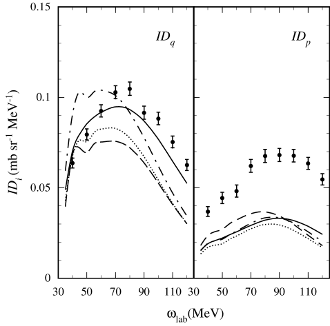
FIG. 1.: DWIA results of $ID_{q}$ and $ID_{p}$ for ¹²C($\vec{p},\vec{n}$) at 494 MeV. The dashed line denotes the result with $m^{*}=m$ and without the RPA correlation. The dotted and the dot-dashed lines represent the RPA results of $(g^{\prime}_{NN},g^{\prime}_{N\Delta},g^{\prime}_{\Delta\Delta})=(0.6,0.6,0.6)$ and $(0.6,0.3,0.5)$ with $m^{*}=m$, respectively. The solid line shows the RPA results of $(0.6,0.3,0.5)$ with $m^{*}(r=0)=0.7m$. Experimental data are taken from Taddeucci et al.[8]

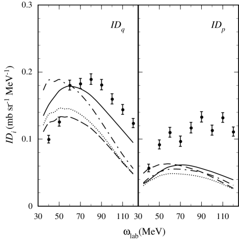
FIG. 2.: The same as Fig.1,but for ⁴⁰Ca($\vec{p},\vec{n}$).

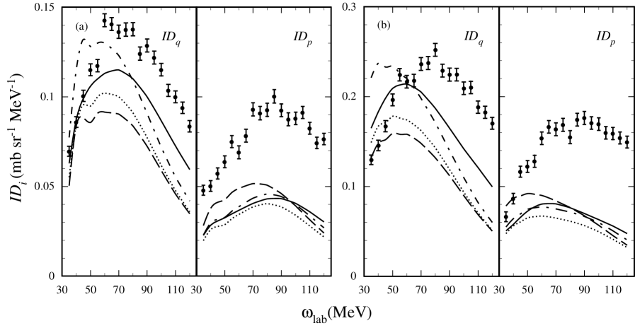
FIG. 3.: The same as Fig.1, but for (a) ¹²C($\vec{p},\vec{n}$) and (b) ⁴⁰Ca($\vec{p},\vec{n}$) at 346 MeV. The experimental data are taken from Wakasa et al.[9]

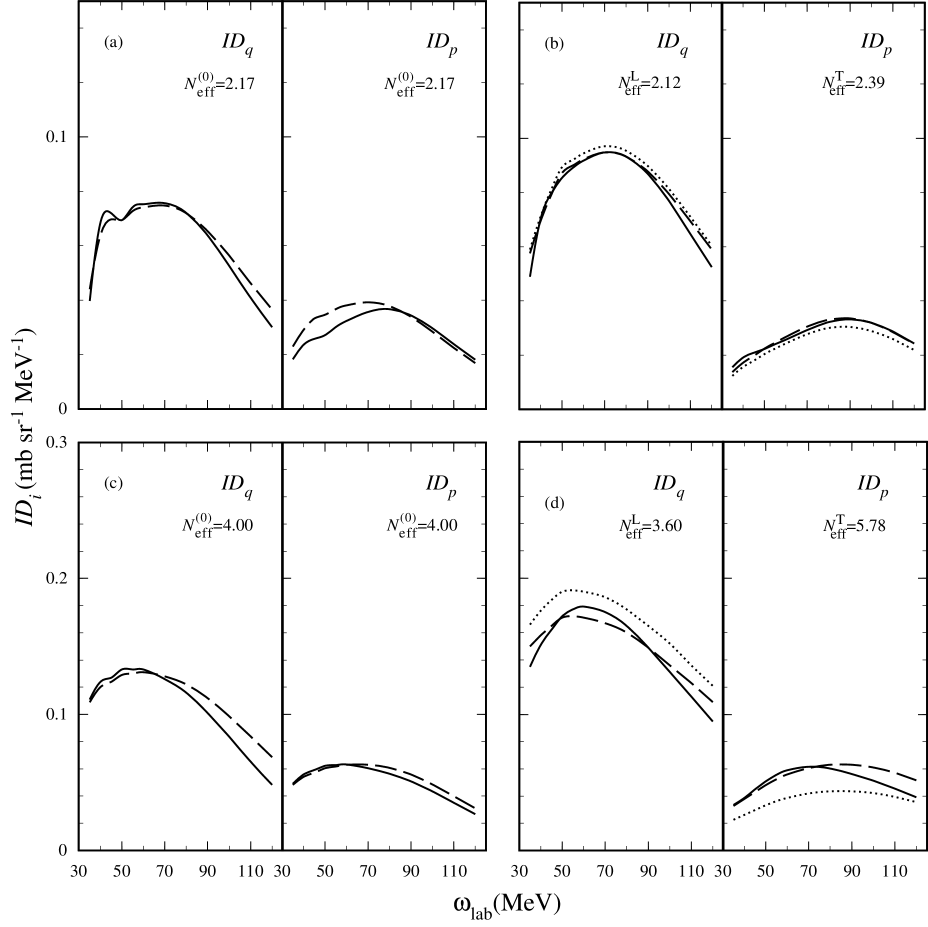
FIG. 4.: Comparison of DWIA and PWIA results at 494 MeV: (a) without and (b) with the RPA correlation for ¹²C($\vec{p},\vec{n}$) and (c) without and (d) with the RPA correlation for ⁴⁰Ca($\vec{p},\vec{n}$). The solid and the dashed lines denote the DWIA and the PWIA results multiplied by $N^{(0)}_{\rm eff}/N(=N_{\rm eff}/N)$ in (a) and (c) and by $N^{\rm L(T)}_{\rm eff}/N$ in (b) and (d) , respectively. The dotted lines denote the PWIA results multiplied by $N_{\rm eff}/N$ in (b) and (d). The values of $N^{(0)}_{\rm eff}$ and $N^{\rm L(T)}_{\rm eff}$ are shown in the figure.

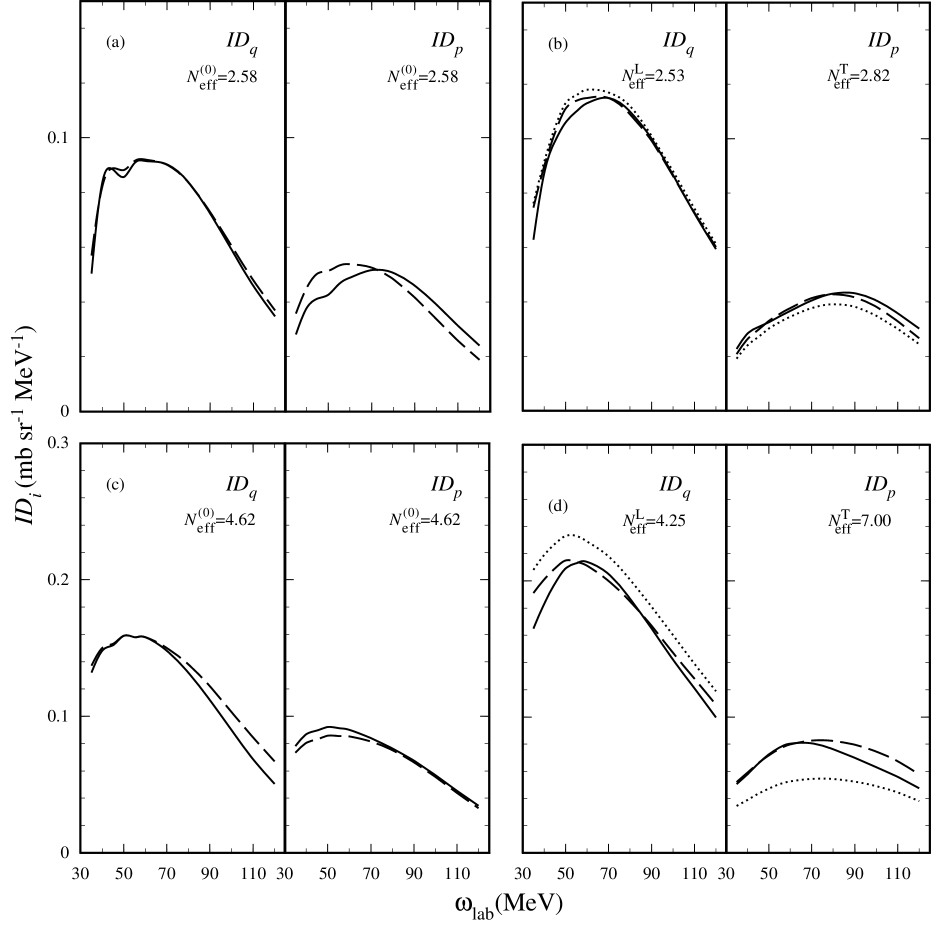
FIG. 5.: The same as Fig.4, but at 346 MeV.

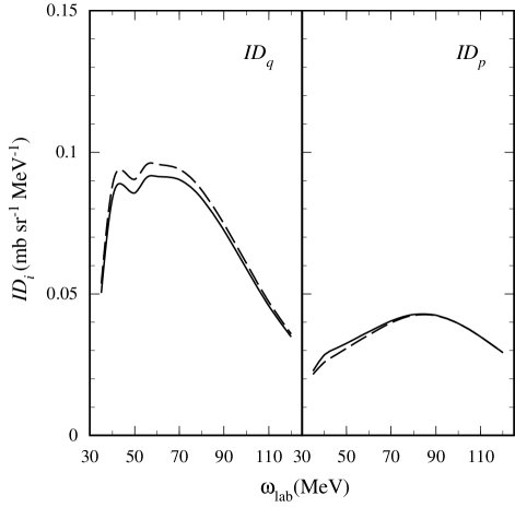
FIG. 6.: Comparison of the DWIA results with (full line) and without (dashed line) the spin orbit force for ¹²C($\vec{p},\vec{n}$) at 346 MeV.

FIG. 7.: Comparison of the results with various optical potentials for ¹²C($\vec{p},\vec{n}$) at 346 MeV. The full lines denote the results with the potential obtained by Cooper et al.[42] for both the proton and the neutron, while the dashed lines denote the results with the potential by Jones et al.[43] for the proton and by Shen et al.[44] for the neutron.

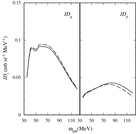
FIG. 8.: Comparison of the results with the $NN$ amplitudes given by Bugg and Wilkin (full line)[51] and by Arndt (dashed line)[52] for ¹²C($\vec{p},\vec{n}$) at 346 MeV.