Improvement of the extended P+QQ interaction by modifying the monopole field

Abstract

The extended pairing plus $QQ$ interaction with the $J$-independent isoscalar proton-neutron force as an average monopole field, which has succeeded in describing collective yrast states of $N\approx Z$ even-$A$ nuclei, is improved. The improvement is accomplished by adding small monopole terms (relevant to spectroscopy) to the average monopole field (indispensable to the binding energy). This modification extends the applicability of the interaction to nuclei with $N\approx 28$ such as ⁴⁸Ca, and moreover improves energy levels of noncollective states. The modified interaction successfully describes not only even-$A$ but also odd-$A$ nuclei in the $f_{7/2}$ shell region. Results of exact shell model calculations in the model space ($f_{7/2}$, $p_{3/2}$, $p_{1/2}$) (its usefulness has been demonstrated previously) are shown for $A$=47, 48, 49, 50 and 51 nuclei.

PACS: 21.60.-n;21.10.Dr;21.10.Hw;21.10.Re

, and

1 Introduction

An extended $P+QQ$ force model [1, 2] has been applied to even-$A$ nuclei in the $f_{7/2}$ shell region, in the previous paper [3] (hereafter referred to as (I)). The exact shell model calculations have shown that the $P_{0}+P_{2}+QQ+V^{0}_{\pi\nu}$ interaction well reproduces the observed energy levels and $E2$ transition probabilities of the collective yrast states as well as the binding energies in the $A$=46, 48 and 50 nuclei with $N\approx Z$. The correspondence between theory and experiment is almost comparable to that attained by the full $fp$ shell model calculations with realistic effective interactions [4, 5, 6, 7, 8, 9, 10].

The $P_{0}+QQ$ or $P_{0}+P_{2}+QQ$ force [11, 12, 13, 14] has been regarded as a schematic interaction which represents typical correlations in nuclei. The results in (I), however, told us that the extended $P+QQ$ force accompanied by the $J$-independent proton-neutron ($p$-$n$) force $V^{0}_{\pi\nu}$ is more than a mere schematic interaction and reflects the important aspects of the real interaction. The interaction serves for quantitative description of nuclear structure in the $fp$ shell region. This conclusion is consistent with the discussion of Dufour and Zuker [15] that the residual part of a realistic effective interaction obtained after extracting the monopole terms is dominated by the multipole forces ($P_{0}$, $QQ$ etc.). In our model, the $V^{0}_{\pi\nu}$ force nicely plays the role of the average monopole field and recovers the deficiency of the binding energy given by the $P_{0}+P_{2}+QQ$ force.

The calculated results in (I), however, revealed two flaws of the $P_{0}+P_{2}+QQ+V^{0}_{\pi\nu}$ interaction: (1) noncollective states except the collective yrast states have a tendency to go down; (2) binding energies and level schemes become worse as $N$ separates from $Z$, especially when $N$ is close to 28 as ⁴⁸Ca. These flaws remind us of the divergence from experiment when the Kuo-Brown (KB) interaction [16] is applied to systems of many valence nucleons ⁴⁸Ca, ⁴⁹Ca etc [17]. The divergence was cured by modifying the monopole components of the $T=0$ and $T=1$ interaction matrix elements [18, 19]. The power of the modified interaction KB3 [4, 19] was shown in the exact shell model calculations [4, 5, 6, 20, 21]. The modified aspect of another effective interaction FPD6 [22] refers also to the monopole terms [23]. These indicate the importance of the monopole terms in spectroscopy [15, 18, 19, 23, 24]. Our interaction has the most important term $V^{0}_{\pi\nu}$ as the average monopole field but does not include the monopole terms which affect spectroscopy. It is a natural next concern to investigate whether the additional monopole terms can remove or not the flaws mentioned above.

For this purpose, we carry out exact shell model calculations in the same model space ($f_{7/2},p_{3/2},p_{1/2}$) as in (I), where the model space was shown to be useful when the average monopole field ($V^{0}_{\pi\nu}$) independent of the extent of space is properly treated [3]. We introduce additional monopole terms so that their forms are as simple as possible and the number of new parameters is minimal. The modified interaction gives us satisfactory results for the $f_{7/2}$ shell nuclei. This paper presents only a short review for even-$A$ nuclei, because the conclusions in (I) for the collective yrast states of $N\approx Z$ even-$A$ nuclei are hardly changed. Our major attention is devoted to odd-$A$ nuclei, the structure of which is expected to be sensitive to the effective interaction employed. There are successful works by Martínez-Pinedo et al. [20, 21] in which the $A$=47 and 49 nuclei are exhaustively studied by the full $fp$ shell model with the KB3 interaction. We examine the quality of our model by comparing our results with theirs as well as experimental ones. We shall also show that our model describes $A$=51 nuclei very well.

In Section 2, the additional monopole terms are introduced into our model and new parameters are determined for ⁴⁸Ca and ⁴⁷Ti. Section 3 makes a report about the effects of the modification on even-$A$ nuclei. Section 4 examines the results of calculations in the cross conjugate nuclei (⁴⁷Ti, ⁴⁹V) and (⁴⁷V, ⁴⁹Cr). The results for $A$=51 are shown in Section 5. Concluding remarks are given in Section 6.

2 modification of the monopole filed

We start with the same model as in (I), i.e., the $P_{0}+P_{2}+QQ+V^{0}_{\pi\nu}$ interaction in the model space $(f_{7/2},p_{3/2},p_{1/2})$ with the following parameter set called ”Set A” in this paper (see (I) in detail):

Set A: $$\varepsilon_{7/2}=0.0,\quad\varepsilon_{3/2}=1.98,\quad\varepsilon_{1/2}=3.61,$$ (1)

$$g_{0}=0.48(42/A),\quad\ g_{2}=0.36(42/A)^{5/3},$$

$$\chi^{\prime}=0.30(42/A)^{5/3},\quad k^{0}=2.23(42/A)\quad\mbox{(in MeV).}$$

This model succeeds in describing the collective yrast states of $N\approx Z$ nuclei, but cannot well reproduce binding energies and level schemes in nuclei with $N\approx 28$. We consider ⁴⁸Ca as a conspicuous example in Fig. 1. The ground-state energy calculated with the parameter set A is -3.72 MeV against the experimental energy -7.04 MeV. The obtained level scheme is shown in the first column A in Fig. 1. There is a significant discrepancy between the original model (column A) and experiment (column exp).

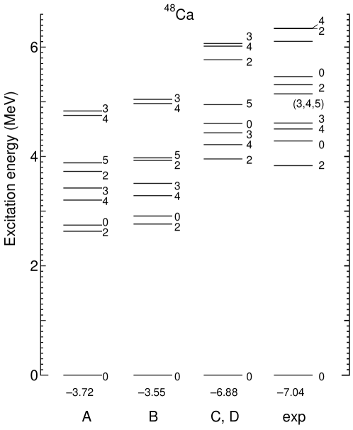
Figure 1: Energy levels of ⁴⁸Ca calculated with four different sets of parameters, compared with the observed levels. The ground-state energy is also shown below the $0^{+}_{1}$ level in MeV.

We used the naive single-particle energies with small spaces from the observed levels of ⁴¹Ca in the Set A. One may attribute the lowering of excited states to the small spaces $\epsilon_{7/2}-\epsilon_{3/2}$ and $\epsilon_{7/2}-\epsilon_{1/2}$. The single-particle energies, however, do not very much affect the level scheme in the $P_{0}+P_{2}+QQ$ force model, as mentioned in (I). If a little strengthened $QQ$ force is used for the single-particle energies of Kuo and Brown [16], energy levels obtained are almost unchanged for the collective states in $N\approx Z$ nuclei. The effect on ⁴⁸Ca is shown in the second column B of Fig. 1. The small energy gap between $0^{+}_{1}$ (the ground state) and $2^{+}_{1}$ is little improved. The use of the Kuo-Brown single-particle energies which are often employed will be convenient for comparison of our interaction with other effective interactions. We therefore use the new set of parameters (called ”Set B”) for the $P_{0}+P_{2}+QQ$ force in this paper,

Set B: $$\varepsilon_{7/2}=0.0,\quad\varepsilon_{3/2}=2.1,\quad\varepsilon_{1/2}=3.9,$$ (2)

$$g_{0}=0.48(42/A),\quad\ g_{2}=0.36(42/A)^{5/3},$$

$$\chi^{\prime}=0.31(42/A)^{5/3},\quad k^{0}=2.23(42/A)\quad\mbox{(in MeV).}$$

In ⁴⁸Ca, the dominant component of the ground state $0^{+}_{1}$ is the neutron configuration $(f_{7/2})^{8}$, and main components of the lowest excited states are $(f_{7/2})^{7}(p_{3/2})$ and $(f_{7/2})^{7}(p_{1/2})$. The deep binding energy of $0^{+}_{1}$ is probably due to the large correlation energy of the closed subshell configuration $(f_{7/2})^{8}$, which is given by

$$\sum_{J=\mbox{even}}(2J+1)\langle f_{7/2}f_{7/2}J,T=1|V|f_{7/2}f_{7/2}J,T=1\rangle.$$ (3)

If we enlarge the value of Eq. (3), we can get a deep binding energy of ⁴⁸Ca. The enlargement of the $f_{7/2}$ interaction matrix elements gives a smaller energy gain to the excited states than $0^{+}_{1}$, and hence extends the energy gap between $2^{+}_{1}$ and $0^{+}_{1}$. The $2^{+}_{1}-0^{+}_{1}$ energy gap is further increased by weakening the interaction matrix elements $\langle f_{7/2}rJ,T=1|V|f_{7/2}rJ,T=1\rangle$ ($r=p_{3/2}$ or $p_{1/2}$). Note that only the isovector interactions with $T=1$ take action in ⁴⁸Ca.

Therefore, a simple way to improve the binding energy and level scheme of ⁴⁸Ca is to add the following correction to the isovector $(T=1)$ interactions:

$$\sum_{ab}\sum_{J}\Delta k^{1}(abJ)\sum_{M\kappa}A^{+}_{JM1\kappa}(ab)A_{JM1\kappa}(ab),$$ (4)

where $A^{\dagger}_{JM\tau\kappa}(ab)=[c_{a}^{\dagger}c_{b}^{\dagger}]_{JM\tau\kappa}/\sqrt{1+\delta_{ab}}$. Neglecting the $J$-dependence of $\Delta k^{1}(abJ)$, in this paper, we make further simplification

$$\Delta k^{1}(abJ)=\left\{\begin{array}[]{ll}\Delta k^{1}(f_{7/2}f_{7/2})&\mbox{ for }a=b=f_{7/2}\\ \Delta k^{1}(f_{7/2}r)&\mbox{ for }r=p_{3/2}\mbox{ or }p_{1/2}\\ 0&\mbox{ for the others.}\end{array}\right.$$ (5)

Then, we have the isovector correction $\Delta V^{1}$ which belongs to the monopole terms discussed in Refs. [4, 15, 24],

$$\Delta V^{1} = \Delta k^{1}(f_{7/2}f_{7/2})\sum_{J=\mbox{even}}\sum_{M\kappa}A^{\dagger}_{JM1\kappa}(f_{7/2}f_{7/2})A_{JM1\kappa}(f_{7/2}f_{7/2})$$ (6)

$$+ \Delta k^{1}(f_{7/2}r)\sum_{b\in r}\sum_{J}\sum_{M\kappa}A^{\dagger}_{JM1\kappa}(f_{7/2}b)A_{JM1\kappa}(f_{7/2}b).$$

We can expect $\Delta k^{1}(f_{7/2}f_{7/2})$ being attractive and $\Delta k^{1}(f_{7/2}r)$ being repulsive, from the above consideration. Trial calculations in ⁴⁸Ca recommend the following corrections to the parameter set B, which we call ”Set C”:

Set C: Set B accompanied by the corrections (7)

$$\Delta k^{1}(f_{7/2}f_{7/2})=-0.14,\quad\Delta k^{1}(f_{7/2}r)=0.05\quad\mbox{(in MeV)}.$$

The parameter set C yields the level scheme in the third column C of Fig. 1. The agreement with the observed levels is satisfactory. Figure 1 testifies that the $P_{0}+P_{2}+QQ$ force is very much improved by adding the isovector monopole terms as Eq. (6).

Figure 2: Energy levels of ⁴⁷Ti calculated with four different sets of parameters, compared with the observed levels. The ground-state energy is also shown below the $0^{+}_{1}$ level in MeV.

Let us test the validity of $\Delta V^{1}$ with the parameters (7) in odd-$A$ nuclei which are sensitive to the interaction employed. Figure 2 illustrates the comparison between calculated yrast levels and observed ones in ⁴⁷Ti, where only negative-parity states are considered in our model space $(f_{7/2},p_{3/2},p_{1/2})$. The results in the columns A, B and C are obtained by using the parameter sets A, B and C, respectively. The results A and B show that the $P_{0}+P_{2}+QQ$ force fairly well reproduces the collective ground-state band on the $5/2^{-}$ state but lays the noncollective low-spin states $3/2^{-}$ and $1/2^{-}$ too much lower. This tendency is one of the flaws of the $P_{0}+P_{2}+QQ$ force. The column C indicates that the isovector monopole terms in $\Delta V^{1}$ push the $3/2^{-}$ and $1/2^{-}$ states up to the correct positions. However, $\Delta V^{1}$ disturbs the order of the adjacent levels $(5/2^{-},7/2^{-})$ and $(9/2^{-},11/2^{-})$ at low energy and lowers the energies of high-spin states above $13/2^{-}$. Furthermore, the introduction of $\Delta V^{1}$ changes the binding energy of not only ⁴⁸Ca but also the other nuclei. Especially, the additional isovector pairing interactions $\langle f_{7/2}f_{7/2}J,T=1|V|f_{7/2}f_{7/2}J,T=1\rangle$ operate on the main configurations of the ground states and cause overbinding.

These secondary troubles can be cured by introducing additional isoscalar $(T=0)$ monopole terms and by weakening the $J$-independent isoscalar force $V^{0}_{\pi\nu}$ (note that they are $p$-$n$ interactions). First, let us write the isoscalar correction $\Delta V^{0}$ in a form similar to $\Delta V^{1}$

$$\Delta V^{0} = \Delta k^{0}(f_{7/2}f_{7/2})\sum_{J=\mbox{odd}}\sum_{M}A^{\dagger}_{JM00}(f_{7/2}f_{7/2})A_{JM00}(f_{7/2}f_{7/2})$$ (8)

$$+ \Delta k^{0}(f_{7/2}r)\sum_{b\in r}\sum_{J}\sum_{M}A^{\dagger}_{JM00}(f_{7/2}b)A_{JM00}(f_{7/2}b).$$

We determine the parameters $\Delta k^{0}(f_{7/2}f_{7/2})$ and $\Delta k^{0}(f_{7/2}r)$ so that the inverse order of $(5/2^{-},7/2^{-})$ and $(9/2^{-},11/2^{-})$ are restored and the high-spin levels get near to the observed ones. Secondly, we weaken the strength $k^{0}$ of $V^{0}_{\pi\nu}$ so as to obtain relatively good binding energies for nuclei from $A$=42 to $A$=51 as a whole. The obtained parameter set, which we call ”Set D”, is

Set D: Set C accompanied by the corrections (9)

$$k^{0}=2.15(42/A),$$

$$\Delta k^{0}(f_{7/2}f_{7/2})=0.18,\quad\Delta k^{0}(f_{7/2}r)=-0.07\quad\mbox{(in MeV)}.$$

Figure 3: Ground-state energies of $A$=42 - 51 nuclei calculated with the original model A and modified one D, and the experimental energies. The experimental energies of the corresponding isobaric analogue states are also plotted. For instance, the $T=4$ states at $A$=48 show the ground state of ⁴⁸Ca and the $T$=4, 0${}^{+}~{}$ states of ⁴⁸Sc and ⁴⁸Ti.

The parameter set D yields the level scheme in the fourth column D of Fig. 2. The energy levels of the ground-state band are well reproduced as those of the original model A and the $3/2^{-}$ and $1/2^{-}$ levels lie at good positions. The agreement with the observed levels is considerably good. The $p$-$n$ interactions $\Delta V^{0}$ and $V^{0}_{\pi\nu}$ do not affect the spectrum of the ⁴⁸Ca nucleus which has only valence neutrons. The third column of Fig. 1 for ⁴⁸Ca is nothing but the result obtained by using the parameter set D. We can determine the strengths of $\Delta k^{0}(f_{7/2}f_{7/2})$ and $\Delta k^{0}(f_{7/2}r)$ also in ⁴⁶V, because the relative energy of the lowest $T=0$ and $T=1$ states in odd-odd nuclei is sensitive to these parameters. If we enlarge the absolute values of $\Delta k^{0}(f_{7/2}f_{7/2})$ and $\Delta k^{0}(f_{7/2}r)$, we get better energies for $T=0$ low-spin states but too high energies for $T=0$ high-spin states in ⁴⁶V. The same tendency is seen in the column D of Fig. 2, where the larger the values of $\Delta k^{0}(f_{7/2}f_{7/2})$ and $\Delta k^{0}(f_{7/2}r)$ become, the higher the high-spin levels go up. Figures 1 and 2 say that the parameters $\Delta k^{1}(f_{7/2}f_{7/2})$, $\Delta k^{1}(f_{7/2}r)$, $\Delta k^{0}(f_{7/2}f_{7/2})$ and $\Delta k^{0}(f_{7/2}r)$ must not change too much from the values in Eqs. (7) and (9).

Using the parameter set D, we obtain the ground-state energies shown in Fig. 3, where the obtained result is compared with the result of (I) (cal A) and with the experimental ground-state energies (see (I)). The modification in this paper improves the binding energies of nuclei with large $T$ such as the Ca isotopes, as compared with the original model. Figure 3, however, tells slight overbinding of the $N\approx Z$ nuclei with small $T$. For instance, the model (denoted by +) lowers a little the excitation energies of the $T=1$ and $T=2$ isobaric analogue states in ⁴⁸Cr, while the original model (denoted by $\ast$) reproduces them. We keep the fixed values (7) and (9) of the parameters $\Delta k^{1}$ and $\Delta k^{0}$ for all the $A$=42-51 nuclei in Fig. 3, but the figure suggests that the additional monopole terms are too strong for the $A$=50 and $A$=51 nuclei with large $T$. Possibly the parameters $\Delta k^{1}$ and $\Delta k^{0}$ should have $A$ dependence. The present modification still leaves a room for fine improvement. Our concern is, however, to sketch out functions of various typical interactions. The guiding principle in this paper is to cure the above-mentioned two flaws of the original model by using as few number of parameters as possible. We are content with the results in Figs. 1, 2 and 3. The modified model with the parameter set D fairly well reproduces the binding energies and level schemes of ⁴⁸Ca and ⁴⁷Ti. We shall examine this modified model in the following sections.

3 Effects of the additional monopole terms on even-$A$ nuclei

Let us see the effects of the additional monopole terms on even-A nuclei, to which the original model without these terms is applied in (I).

The original $P_{0}+P_{2}+QQ+V^{0}_{\pi\nu}$ interaction well describes the collective yrast states of $N\approx Z$ even-even nuclei. The additional monopole terms with the parameters (9) have little effect on these nuclei, though we do not show figures of the results except ⁵⁰Cr. The discussions about the collective yrast states of ⁴⁶Ti, ⁴⁸Cr and ⁵⁰Cr in (I) remain valid also in the present modified model. The level structure including non-yrast levels and $B(E2)$ in the ground-state band are hardly changed in ⁴⁶Ti and ⁴⁸Cr. The backbending plot of the ⁴⁸Cr rotational band is fairly well and the quality is the same as that in (I). Speaking strictly, the additional monopole terms do not improve the excitation energies of $8^{+}_{1}$, $10^{+}_{1}$ and $12^{+}_{1}$ in the backbending region. The somewhat awkward change from the most collective states ($0^{+}_{1}-8^{+}_{1}$) to the high-spin states in the calculated ground-state band of ⁴⁸Cr seems to originate in the $P_{0}+P_{2}+QQ$ force.

Figure 4: Energy levels of ⁵⁰Cr calculated with the original and modified models (A and D), compared with the observed levels.

The modified model (D) produces a little better level structure than the original model (A) in ⁵⁰Cr, as shown in Fig. 4. Not only the yrast levels but also other levels correspond better to the observed levels. The low-spin states $2^{+}_{2}$, $4^{+}_{2}$, $2^{+}_{3}$ and $0^{+}_{2}$, and the high-spin states $13^{+}_{2}$, $13^{+}_{3}$, $14^{+}_{2}$, $14^{+}_{3}$, $15^{+}_{2}$, $15^{+}_{3}$, $16^{+}_{2}$ and $17^{+}_{2}$ come nearer to the observed positions. In ⁵⁰Cr, however, the $B(E2)$ values between the most collective yrast states are considerably reduced: $B(E2:J_{1}\rightarrow(J-2)_{1})$ in e²fm⁴ is 197 for $J=2$; 277 for $J=4$; 122 for $J=6$; 121 for $J=8$ in the calculation D, while it is 215 for $J=2$; 302 for $J=4$; 211 for $J=6$; 200 for $J=8$ in the calculation A. The modification of the model has a tendency to push high-spin yrast states upward, as seen in Fig. 4. The same tendency is observed in the results of ⁴⁶Ti and ⁴⁸Cr.

Figure 5: Energy levels of ⁵⁰Ti calculated with the original and modified models (A and D), compared with the observed levels.

The modified model works clearly better as compared with the original model, when $N$ separates from $Z$, as in ⁴⁸Ca. We show the level scheme of ⁵⁰Ti as a good example in Fig. 5, where yrast levels and other low-lying levels obtained by the original model (A) and modified one (D) are compared with the observed levels. The additional monopole terms move the yrast levels above $5^{+}_{1}$ very nearer to the observed ones, and push the non-yrast levels upward, laying them at good positions.

Figure 6: Energy levels of ⁵⁰Mn calculated with the original and modified models (A and D), compared with the observed levels.

Figure 7: Energy levels of ⁴⁸Sc calculated with four different sets of parameters, compared with the observed levels.

Next, we examine the applicability of our modified model in odd-odd nuclei which are most sensitive to the interaction employed. The previous paper (I) has shown that the $P_{0}+P_{2}+QQ+V^{0}_{\pi\nu}$ interaction can describe the yrast level structure in ⁴⁶V, ⁴⁸V and ⁵⁰Mn beyond expectation. The introduction of the additional monopole terms reproduces relatively better results in these nuclei. In ⁴⁶V, for instance, the lowest $3^{+}$ state with $T=0$ lies at 0.24 MeV in the original model A, while it lies at 0.59 MeV, coming near to the observed excitation energy 0.80 MeV, in the modified model D. The yrast and non-yrast levels correspond better to the observed ones in the present modified model, though the high-spin state $15^{+}_{1}$ goes up a little.

As shown in Fig. 6, the relative positions of the $T=0$ and $T=1$ states are improved also in ⁵⁰Mn. The original model (A) lays the lowest $T=0$ state with $J^{\pi}=1^{+}$ below the $T=1$, $0^{+}_{1}$ state, but the modified model (D) correctly yields the ground state with $T=1$, $J^{\pi}=0^{+}$. If we regard the $T=0$ yrast levels with $J\geq 5$ as a collective band on the band-head state $5^{+}_{1}$, the band is well reproduced by our model. The additional monopole terms push non-yrast (noncollective) levels toward the observed ones. The yrast states with smaller spins ($J<5$) than the band-head state, however, remain at low energy, and hence the order of low-lying levels does not correspond to the experimental order.

The same problem is observed in odd-odd nuclei away from $N=Z$, though the introduction of the additional monopole terms is very effective in improving the level scheme. The modified model well describes the collective yrast band, but cannot reproduce the correct order of low-lying levels and fails to give the correct ground state in ⁴⁸V and ⁴⁸Sc. In ⁴⁸V, the lowest state $2^{+}_{1}$ is at -0.20 MeV below the ground state $4^{+}_{1}$ in the calculation D. The difference between the calculated and observed yrast levels is 0.5 MeV at most. We show another example in Fig. 7, where results of the calculations A, B, C and D are compared with the observed level scheme of ⁴⁸Sc. Note here that Fig. 7 is drawn in a small-scale as compared with the previous figures. The additional monopole terms produce very improved results. The correspondences of the excitation energies and level density between theory and experiment become better in the modified model D. Although the calculation cannot reproduce the correct ground state, the discrepancy does not exceed 0.4 MeV. The results in odd-odd nuclei suggest that fine improvement would be possible in our extended $P+QQ$ model.

4 Results in the cross-conjugate nuclei ⁴⁷Ti - ⁴⁹V and ⁴⁷V - ⁴⁹Cr

The accumulation of experimental and theoretical studies has been clarifying the structure of $A$=47 and $A$=49 nuclei. Martínez-Pinedo et al. [20, 21] made an exhaustive study of these nuclei by the full $fp$ shell model calculation using the KB3 interaction. These nuclei are very suitable for examining the quality of our model. We direct our attention to the pairs of nuclei ⁴⁷Ti - ⁴⁹V and ⁴⁷V - ⁴⁹Cr which have the cross-conjugate configurations ($(f_{7/2})^{7p}$ and $(f_{7/2})^{7h}$) in the single $j$ limit. The energy levels of ⁴⁷V and ⁴⁷Cr (⁴⁹Cr and ⁴⁹Mn) are equivalent in our model because of the isospin invariant Hamiltonian. We discuss the structure of ⁴⁷V and ⁴⁹Cr for simplicity. Only negative-parity states of these nuclei are considered in the model space. We use the effective charge $e_{eff}=0.5e$ and the harmonic-oscillator range parameter $b_{0}=1.01A^{1/6}$ fm in the calculations. These values are the same as those in Refs. [20, 21].

4.1 ⁴⁷Ti - ⁴⁹V

We have already seen in Fig. 2 that the extended $P+QQ$ model satisfactorily reproduces the yrast levels of ⁴⁷Ti. This is clearer in the spin-energy graph in Fig. 8, where our model (cal D) correctly traces the observed staggering gait depending on the spins $(2J\pm 1)/2$. The result of our extended $P+QQ$ model is almost comparable to that of Martínez-Pinedo et al. with the KB3 interaction. The KB3 interaction reproduces better the $17/2^{-}_{1}$, $19/2^{-}_{1}$ and $21/2^{-}_{1}$ levels than ours, while our interaction correctly reproduces the order of $9/2^{-}_{1}$ and $11/2^{-}_{1}$ and the position of the high-spin level $27/2^{-}_{1}$ as compared with the KB3. The insufficiency of our model with respect to the energy of $21/2^{-}_{1}$ is possibly related to the remaining flaw around $8^{+}_{1}-12^{+}_{1}$ in ⁴⁸Cr mentioned in the previous section. The staggering in the spin-energy graph of Fig. 8 reminds us of that in the odd-odd nuclei ⁴⁶V, ⁴⁸V and ⁵⁰Mn discussed in (I). There must be a similar mechanism of excitation (rotation) in the yrast bands of ⁴⁷Ti and ⁴⁸V.

Figure 8: Theoretical and experimental spin-energy relation in the yrast band of ⁴⁷Ti. The result of the full $fp$ shell model calculation with the KB3 interaction [20] is also shown by the dotted line.

Table 1 shows electric quadrupole properties of the yrast and other states in ⁴⁷Ti. The calculated $B(E2)$ values correspond to the tendency of the observed ones [27] to some extent, but the quality of the data may not be sufficient [20]. We calculated the spectroscopic quadrupole moment $Q_{spec}$ and intrinsic quadrupole moments $Q^{(s)}_{0}$ and $Q^{(t)}_{0}$ for the yrast states in addition to $B(E2)$. (We use the same notations $Q^{(s)}_{0}$ and $Q^{(t)}_{0}$ as Martínez-Pinedo et al. [20].) With respect to these electric quadrupole properties, our predictions in the smaller model space $(f_{7/2},p_{3/2},p_{1/2})$ are very similar to those of the full $fp$ shell model with the KB3 interaction.

Table 1: Electric quadrupole properties of the yrast and other states in ⁴⁷Ti: ${B(E2)}$ in $e^{2}$ fm⁴; $Q_{spec}$, $Q^{(s)}_{0}$ and $Q^{(t)}_{0}$ in $e$ fm². The present results are compared with the experimental ones and those of Martínez-Pinedo et al.

	Expt.	present				Martínez-Pinedo
$J_{n}\rightarrow J^{\prime}_{m}$	$B(E2)$	$B(E2)$	$Q_{spec}$	$Q^{(s)}_{0}$	$Q^{(t)}_{0}$	$B(E2)$	$Q^{(s)}_{0}$	$Q^{(t)}_{0}$
$5/2_{1}$			23.6	66			63.4
$7/2_{1}\rightarrow 5/2_{1}$	252(50)	145	6.4	96	64	140	120.3	61.6
$9/2_{1}\rightarrow 5/2_{1}$	70(30)	56	-5.5	61	75	55	44.1	72.7
$\rightarrow 7/2_{1}$	191(40)	136			67	102		57.1
$11/2_{1}\rightarrow 7/2_{1}$	159(25)	98	-6.8	36	76	98	10.9	74.7
$\rightarrow 9/2_{1}$	705(605)	92			63	83		58.6
$13/2_{1}\rightarrow 9/2_{1}$		109	-14.3	57	71		60.7	67.5
$\rightarrow 11/2_{1}$		68			62			57.3
$15/2_{1}\rightarrow 11/2_{1}$	135(26)	102	-11.5	39	64	111	29.8	66.0
$\rightarrow 13/2_{1}$		47			58			50.2
$17/2_{1}\rightarrow 13/2_{1}$		89	-19.6	60	58		69.7	59.7
$\rightarrow 15/2_{1}$	604${}^{+70}_{-640}$	34			55	41		59.3
$19/2_{1}\rightarrow 15/2_{1}$		57	-19.4	55	45		45.6	51.9
$\rightarrow 17/2_{1}$	$<50$	30			57	25		50.6
$21/2_{1}\rightarrow 17/2_{1}$		41	-21.1	57	37		66.6	40.4
$\rightarrow 19/2_{1}$		7			30			40.3
$23/2_{1}\rightarrow 19/2_{1}$		43	-19.6	51	38		53.5	43.1
$\rightarrow 21/2_{1}$		21			56			56.8
$25/2_{1}\rightarrow 21/2_{1}$		12	-10.2	26	19		30.1	20.3
$\rightarrow 23/2_{1}$		1.4			16			9.1
$27/2_{1}\rightarrow 23/2_{1}$		25	-17.5	43	28		46.7	28.8
$\rightarrow 25/2_{1}$		19			62			65.8
$3/2_{1}\rightarrow 5/2_{1}$	3.3(15)	9.9				22
$\rightarrow 7/2_{1}$	39(11)	1.4				46
$1/2_{1}\rightarrow 5/2_{1}$	$<17$	11				21
$3/2_{2}\rightarrow 5/2_{1}$	$<272$	9.4				0.48
$\rightarrow 7/2_{1}$	36.3(70)	60				8.3

For the ground state $5/2^{-}_{1}$, The calculated spectroscopic quadrupole moment $Q_{spec}=23.6$ $e$ fm² is nearly equal to the value 22.7 $e$ fm² of Ref. [20] but does not well reproduce the observed value 30.3 $e$ fm². The calculated results show that $B(E2:J\rightarrow J-1)$ is larger than $B(E2:J\rightarrow J-2)$ up to $J=9/2$, while $B(E2:J\rightarrow J-2)$ exceeds $B(E2:J\rightarrow J-1)$ above $J=9/2$ in the yrast band. The full $fp$ shell model with the KB3 interaction seems to give a similar prediction for the $B(E2)$ ratio from the values of $Q^{(t)}_{0}$. The observed $\gamma$ transitions [26] are consistent with the theoretical prediction up to $15/2^{-}_{1}$ but show a different feature from the prediction for $J\geq 17/2^{-}_{1}$. In the calculation, $Q_{spec}$ changes the value considerably at $17/2^{-}_{1}$ and above it the $B(E2)$ values become smaller. Our model gives different $B(E2)$ values to the $3/2^{-}_{1}$ and $1/2^{-}_{1}$ states from Ref. [20].

Figure 9: Calculated and observed energy levels of ⁴⁹V. The lowest two levels of each $J$ (yrast and $J_{2}$) obtained by the present model are compared with the observed ones. The yrast levels obtained by the full $fp$ shell model calculation with the KB3 interaction [20] are shown by the dotted line.

Energy levels of ${}^{49}_{23}$V₂₆ obtained by the present model are compared with observed levels [25, 28] in Fig. 9. Our model reproduces not only the yrast levels but also the second lowest levels from $J^{\pi}=3/2^{-}$ to $11/2^{-}$, and nearly traces the staggering gait in the spin-energy graph of the yrast states. For the yrast levels, the correspondence between theory and experiment in ⁴⁹V is somewhat worse than that in ⁴⁷Ti at high spin. It is, however, notable that the two spin-energy graphs of the cross-conjugate nuclei ⁴⁷Ti and ⁴⁹V in Figs. 8 and 9 resemble each other and are well described by our model.

Table 2: Electric quadrupole properties of the yrast and other states in ⁴⁹V: ${B(E2)}$ in $e^{2}$ fm⁴; $Q_{spec}$ in $e$ fm².

	Expt.	present		Martínez-Pinedo
$J_{n}\rightarrow J^{\prime}_{m}$	$B(E2)$	$B(E2)$	$Q_{spec}$	$B(E2)$	$Q_{spec}$
$7/2_{1}$			-12.2		-11.1
$5/2_{1}\rightarrow 7/2_{1}$		246	-7.3
$3/2_{1}\rightarrow 5/2_{1}$		355	19.5
$\rightarrow 7/2_{1}$	204(6)	205		196
$11/2_{1}\rightarrow 7/2_{1}$	149(27)	158	-20.7	157
$9/2_{1}\rightarrow 5/2_{1}$	84(24)	116	-25.4	88
$\rightarrow 7/2_{1}$	63(19)	70		41
$\rightarrow 11/2_{1}$		98
$15/2_{1}\rightarrow 11/2_{1}$	298${}^{+85}_{-180}$	107	-2.7	140
$13/2_{1}\rightarrow 9/2_{1}$	290(200)	140	-26.3	110
$\rightarrow 11/2_{1}$		24
$\rightarrow 15/2_{1}$		20
present work
$J_{1}$	$Q_{spec}$	$\rightarrow J^{\prime}_{1}$	$B(E2)$	$\rightarrow J^{\prime}_{1}$	$B(E2)$
$17/2_{1}$	29.3	$\rightarrow 13/2_{1}$	0.9	$\rightarrow 15/2_{1}$	33
$19/2_{1}$	7.1	$\rightarrow 15/2_{1}$	13	$\rightarrow 17/2_{1}$	79
$21/2_{1}$	10.6	$\rightarrow 17/2_{1}$	52	$\rightarrow 19/2_{1}$	42
$23/2_{1}$	0.9	$\rightarrow 19/2_{1}$	68	$\rightarrow 21/2_{1}$	55
$25/2_{1}$	-2.9	$\rightarrow 21/2_{1}$	44	$\rightarrow 23/2_{1}$	37
$27/2_{1}$	-6.5	$\rightarrow 23/2_{1}$	43	$\rightarrow 25/2_{1}$	24

Table 2 shows calculated $B(E2)$ values and observed ones [29], and calculated values of the spectroscopic quadrupole moment $Q_{spec}$. The results of Martínez-Pinedo et al. [20] are also shown for comparison. The $B(E2)$ values obtained by our model are comparable with those of Ref. [20], and roughly consistent with the observed $B(E2)$ values though the data are of poor quality. The spectroscopic quadrupole moment of the ground state $7/2^{-}_{1}$ obtained by our model is nearly equal to that of Ref. [20]. The calculated values of $Q_{spec}$ say that the yrast band changes the structure at the $17/2^{-}_{1}$ state. Correspondingly, the absolute $B(E2)$ values and the ratio $B(E2:J_{1}\rightarrow(J-2)_{1})/B(E2:J_{1}\rightarrow(J-1)_{1})$ show different features before and after $17/2^{-}_{1}$. This structure change appears in the spin-energy graph of Fig. 9, where the staggering is large from $9/2^{-}_{1}$ to $11/2^{-}_{1}$ and from $13/2^{-}_{1}$ to $15/2^{-}_{1}$, and then becomes gentle above the $15/2^{-}_{1}$ state, both in theory and experiment.

4.2 ⁴⁷V - ⁴⁹Cr

Figure 10 shows calculated energy levels and observed ones [25, 26, 30, 31] of ${}^{47}_{23}$V₂₄: the yrast levels and other low-lying levels. The experimental energy of the $21/2^{-}_{1}$ state shown in Fig. 10 is chosen from Ref. [31], which is different from that of Ref. [30]. The present model excellently reproduces the yrast levels up to the $23/2^{-}$ state. The correspondence between theory and experiment with respect to other low-lying states is also considerably well. Our model reproduces better the high-spin levels $27/2^{-}_{1}$ and $29/2^{-}_{1}$ than the full $fp$ shell model with the KB3 interaction [20, 21], and correctly yields the regular order of the pair levels ($25/2^{-}_{1}$, $27/2^{-}_{1}$) and the inverse order of ($31/2^{-}_{1}$, $29/2^{-}_{1}$). However, the observed staggering gait from $25/2^{-}_{1}$ to $31/2^{-}_{1}$ in the spin-energy graph is not well reproduced in contrast to the success of Refs. [20, 21]. This is a question to our model which is expected to describe the collective band well. We shall touch upon this question in the next subsection.

Figure 10: Calculated and observed energy levels of ⁴⁷V. The yrast levels obtained by the full $fp$ shell model calculation with the KB3 interaction [20] are shown by the dotted line.

Table 3: Electric quadrupole properties in ⁴⁷V: ${B(E2)}$ in $e^{2}$ fm⁴; $Q_{spec}$ and $Q_{0}$ in $e$ fm².

	Expt.	present				Martínez-Pinedo
$J_{n}\rightarrow J^{\prime}_{m}$	$B(E2)$	$B(E2)$	$Q_{spec}$	$Q^{(s)}_{0}$	$Q^{(t)}_{0}$	$B(E2)$	$Q^{(s)}_{0}$	$Q^{(t)}_{0}$
$3/2_{1}$			19.7	99			100
$5/2_{1}\rightarrow 3/2_{1}$		266	-7.4	104	88	251	138	87
$7/2_{1}\rightarrow 3/2_{1}$	74(10)	105	-13.2	66	86	106	67	88
$\rightarrow 5/2_{1}$		192			95			99
$9/2_{1}\rightarrow 5/2_{1}$	160(50)	137	-25.8	94	80	138	101	82
$\rightarrow 7/2_{1}$		92			81	76		75
$11/2_{1}\rightarrow 7/2_{1}$	200(100)	175	-23.1	72	83	186	69	87
$\rightarrow 9/2_{1}$		87			94			100
$13/2_{1}\rightarrow 9/2_{1}$		167	-31.9	91	78		101	77
$\rightarrow 11/2_{1}$		36			71			66
$15/2_{1}\rightarrow 11/2_{1}$	$<79$ ($>97$)	182	-26.5	71	78		69	81
$\rightarrow 13/2_{1}$		42			88			103
$17/2_{1}\rightarrow 13/2_{1}$		91	-13.3	34	54		-5.5	17
$\rightarrow 15/2_{1}$		4.8			33			22
$19/2_{1}\rightarrow 15/2_{1}$	140(40)	112	-16.1	40	59		39	65
$\rightarrow 17/2_{1}$		2.7			28			106
$21/2_{1}\rightarrow 17/2_{1}$		112	-16.1	40	59		38	54
$\rightarrow 19/2_{1}$		4.0			37			35
$23/2_{1}\rightarrow 19/2_{1}$	93(14)	137	-18.2	43	64		42	66
$\rightarrow 21/2_{1}$		4.3			42			43
$25/2_{1}\rightarrow 21/2_{1}$	10(3)	79	-15.4	36	49		45	57
$\rightarrow 23/2_{1}$		8.7			65			53
$27/2_{1}\rightarrow 23/2_{1}$	117(28)	99	-17.9	41	54		38	55
$\rightarrow 25/2_{1}$		7.8			67			63
$29/2_{1}\rightarrow 25/2_{1}$		32	-15.4	35	31		35	32
$\rightarrow 27/2_{1}$		0.1			7.1			22
$31/2_{1}\rightarrow 27/2_{1}$	55(6)	44	-18.5	42	36		42	41
$\rightarrow 29/2_{1}$		3.6			52			69
$17/2_{2}\rightarrow 13/2_{1}$		55	16.5	-42	42		68	66

In Table 3, calculated electric quadrupole properties $B(E2)$, $Q_{spec}$, $Q^{(s)}_{0}$ and $Q^{(t)}_{0}$ are compared with those of Ref. [20] and with the observed $B(E2)$ values. Our results, which are very similar to those of the full $fp$ shell model calculation with the KB3 interaction except the $17/2^{-}_{1}$ and $17/2^{-}_{2}$ states, correspond well to the observed $B(E2)$ values except $B(E2:25/2^{-}_{1}\rightarrow 21/2^{-}_{1})$. The calculated large values of $B(E2:7/2^{-}_{1}\rightarrow 5/2^{-}_{1})$ and $B(E2:5/2^{-}_{1}\rightarrow 3/2^{-}_{1})$ explain the observed strong $\gamma$ transitions $7/2^{-}_{1}\rightarrow 5/2^{-}_{1}\rightarrow 3/2^{-}_{1}$ [30], and the large values of $B(E2:J^{-}_{1}\rightarrow(J-2)^{-}_{1})$ when $J=11/2$, 15/2, 19/2 and 23/2 are consistent with the observed cascade transitions $23/2^{-}_{1}\rightarrow 19/2^{-}_{1}\rightarrow 15/2^{-}_{1}\rightarrow 11/2^{-}_{1}\rightarrow 7/2^{-}_{1}$ [30, 31]. Other observed $\gamma$ transitions for the high-spin states are not necessarily understood by our result that $B(E2:J^{-}_{1}\rightarrow(J-2)^{-}_{1})$ is much larger than $B(E2:J^{-}_{1}\rightarrow(J-1)^{-}_{1})$ above $7/2^{-}_{1}$. The calculated spectroscopic quadrupole moment $Q_{spec}$ suggests a change in the structure of the yrast band at $17/2^{-}_{1}$, which is consistent with the change appearing near $17/2^{-}_{1}$ in the Coulomb energy difference between the mirror nuclei ⁴⁷V and ⁴⁷Cr [31]. Our model and the full $fp$ shell model with the KB3 interaction give different $Q^{(s)}_{0}$ and $Q^{(t)}_{0}$ for the $17/2^{-}_{1}$ and $17/2^{-}_{2}$ states. The two states in the latter model (where the two are close by) seem to be in reverse order to those in our model. Experimental data about the $17/2^{-}$ states are unfortunately missing for discussing the difference. This is possibly due to the degeneracy of the $17/2^{-}_{1}$ and $19/2^{-}_{1}$ states predicted by our model. The value of $Q_{spec}$ shows a moderate change for the $17/2^{-}_{1}$, $19/2^{-}_{1}$, $23/2^{-}_{1}$, $27/2^{-}_{1}$ and $31/2^{-}_{1}$ states after the structure change (maybe band crossing) at $17/2^{-}_{1}$ in our model.

Figure 11: Calculated and observed energy levels of ⁴⁹Cr. The yrast levels obtained by the full $fp$ shell model calculation with the KB3 interaction [20] are shown by the dotted line.

Table 4: Electric quadrupole properties in ⁴⁹Cr: ${B(E2)}$ in $e^{2}$ fm⁴; $Q_{spec}$ and $Q_{0}$ in $e$ fm².

	Expt.	present				Martínez-Pinedo
$J_{n}\rightarrow J^{\prime}_{m}$	$B(E2)$	$B(E2)$	$Q_{spec}$	$Q^{(s)}_{0}$	$Q^{(t)}_{0}$	$B(E2)$	$Q^{(s)}_{0}$	$Q^{(t)}_{0}$
$5/2_{1}$			35.5	99			101
$7/2_{1}\rightarrow 5/2_{1}$	383(117)	313	8.8	131	94	332	142	98
$9/2_{1}\rightarrow 5/2_{1}$	153(32)	98	-8.5	94	99	97	92	100
$\rightarrow 7/2_{1}$	426(149)	287			98	283		98
$11/2_{1}\rightarrow 7/2_{1}$	184(20)	165	-16.3	87	99	166	69	101
$\rightarrow 9/2_{1}$	107(85)	217			97	213		97
$13/2_{1}\rightarrow 9/2_{1}$	62(27)	199	-25.5	102	96	192	98	96
$\rightarrow 11/2_{1}$	$4^{+106}_{-4}$	157			94	153		94
$15/2_{1}\rightarrow 11/2_{1}$	102(15)	203	-22.6	77	90	185	47	88
$\rightarrow 13/2_{1}$	$<256$	108			88	92		82
$17/2_{1}\rightarrow 13/2_{1}$	70(11)	161	-15.2	46	78		34	75
$\rightarrow 15/2_{1}$		63			83			72
$19/2_{1}\rightarrow 15/2_{1}$	149(32)	128	-6.0	17	67	158	9.8	76
$\rightarrow 17/2_{1}$		51			74			87
$21/2_{1}\rightarrow 17/2_{1}$	0	143	-18.5	50	69		29	66
$\rightarrow 19/2_{1}$		27			59			67
$23/2_{1}\rightarrow 19/2_{1}$		122	-8.8	23	63		13	68
$\rightarrow 21/2_{1}$		22			58			87
$25/2_{1}\rightarrow 21/2_{1}$	90(8)	21	14.4	-36	26		-39	17
$\rightarrow 23/2_{1}$		0.4			8.6			8.6
$27/2_{1}\rightarrow 23/2_{1}$		56	5.1	-12	42		-5.1	52
$\rightarrow 25/2_{1}$		16			58			50
$29/2_{1}\rightarrow 25/2_{1}$	0+84	46	2.2	-5.2	37		-1.4	43
$\rightarrow 27/2_{1}$		15			60			35
$31/2_{1}\rightarrow 27/2_{1}$	$>42$	57	2.5	-6	42		-4.6	42
$\rightarrow 29/2_{1}$		5.2			37			28
$1/2_{1}\rightarrow 5/2_{1}$	$<10$	7.3				7.0
$3/2_{1}\rightarrow 5/2_{1}$	21(6)	3.5				4.1
$\rightarrow 7/2_{1}$	0.26(12)	0.7				4.8

High-spin states of the ${}^{49}_{24}$Cr₂₅ nucleus were identified by recent highly efficient experiments [30, 32]. In Fig. 11, we compare calculated energy levels of ⁴⁹Cr with the observed ones. Our model well describes the energies of the yrast states as a whole. There are slight deviations for the high-spin states $23/2^{-}_{1}$, $25/2^{-}_{1}$ and $29/2^{-}_{1}$. Namely, our model does not reproduce enough the observed magnitudes of the stagger from $21/2^{-}_{1}$ to $23/2^{-}_{1}$ and from $25/2^{-}_{1}$ to $27/2^{-}_{1}$ in the spin-energy graph. The full $fp$ shell model calculation with the KB3 interaction [20] correctly reproduces the inverse order of these pair levels. This is another question to our model, in contrast with the success in ⁴⁷Ti and ⁴⁹V. There is a confusing difference between the spin-energy graphs of the cross conjugate nuclei ⁴⁷V and ⁴⁹Cr. Their staggering gaits up to $19/2^{-}_{1}$ are somewhat different between ⁴⁷V and ⁴⁹Cr, i.e., the energies of the pair states $(4J+1)/2^{-}$ and $(4J+3)/2^{-}$ are close by in ⁴⁷V but are different in ⁴⁹Cr, which is well traced by our model. Above $19/2^{-}_{1}$, our model predicts similar staggering gaits for ⁴⁷V and ⁴⁹Cr (which suggests the dominance of the configurations $(f_{7/2})^{7p}$ and $(f_{7/2})^{7h}$), while the two experimental graphs do not show any regular behavior. This is contrary to the fact that our model well reproduces the yrast bands of the cross-conjugate odd-odd nuclei ⁴⁶V and ⁵⁰Mn (see (I)). The staggering gaits from $25/2^{-}_{1}$ to $27/2^{-}_{1}$ and from $29/2^{-}_{1}$ to $31/2^{-}_{1}$ are asymmetrical between ⁴⁷V and ⁴⁹Cr. The subtle but strange behaviors are curious for us to understand, though the delicate difference in the interaction matrix elements from the realistic effective interaction KB3 could affect the staggering in our model. The interesting fine structure should be investigated further experimentally and theoretically.

Electric quadrupole properties of the yrast states in ⁴⁹Cr are listed in Table 4. The results of our model for $B(E2)$, $Q^{(s)}_{0}$ and $Q^{(t)}_{0}$ are similar to those of Ref. [20]. The calculated $B(E2)$ values are roughly consistent with the observed ones. The calculated spectroscopic quadrupole moment shows a difference between the two sets of the states ($17/2^{-}_{1}$, $21/2^{-}_{1}$) and ($19/2^{-}_{1}$, $23/2^{-}_{1}$), and indicates a distinct change of the structure above $23/2^{-}_{1}$ in the yrast band. This feature is different from that of the cross conjugate nucleus ⁴⁷V but similar to that of ⁴⁹V, which suggests the contribution of the upper orbits above $f_{7/2}$.

Figure 12: Experimental spin-energy relation in the yrast bands of $A$=47 and $A$=49 nuclei.

In Fig. 12, we summarize the observed yrast levels of ⁴⁷Ti, ⁴⁷V, ⁴⁹V and ⁴⁹Cr in the spin-energy graph. The yrast levels appear to be scattered around the $J(J+1)$ curve of the rotation model, where the static moment of inertia is fixed as $I_{mom}$=11 MeV^-1 and the energy of the $5/2^{-}_{1}$ state is set to be zero. This figure indicates a similarity at the beginning of the band on the $5/2^{-}_{1}$ state between ⁴⁷V and ⁴⁹Cr and also between ⁴⁷V and ⁴⁷Ti. Martínez-Pinedo et al. [20] analyzed old data of ⁴⁷V and ⁴⁹Cr by different curves of the $J(J+1)$ law. In our model, the spin-energy graphs of ⁴⁷V and ⁴⁹Cr do not display a very large difference, though the spectroscopic quadrupole moment shows differences as mentioned above ($Q_{spec}$ shows a drastic change at $25/2^{-}_{1}$ in ⁴⁹Cr but not in ⁴⁷V). The asymmetrical positions of ($25/2^{-}_{1}$, $27/2^{-}_{1}$) and ($29/2^{-}_{1}$, $31/2^{-}_{1}$) in ⁴⁷V and ⁴⁹Cr mentioned above are visible in Fig. 12.

5 Results in ⁵¹Mn and ⁵¹Cr

The extended $P+QQ$ model is expected to be applicable to $A=51$ nuclei from Fig. 3. In this section, we show calculated results in ⁵¹Mn and ⁵¹Cr.

Figure 13: Comparison of energy levels between theory and experiment in ⁵¹Mn.

Figure 13 illustrates the comparison of energy levels between the modified model (D) and experiment in ⁵¹Mn. Our model reproduces the collective yrast levels on $5/2^{-}_{1}$ at good energy and in the correct order of spins, except that the space between $15/2^{-}_{1}$ and $17/2^{-}_{1}$ is too narrow. (The awkward reproduction of energy in the middle spin region in our calculation is similar to that in ⁴⁸Cr.) The additional monopole terms improve the positions of the low-spin levels $3/2^{-}_{1}$ and $1/2^{-}_{1}$, the spins of which are smaller than $J=5/2$ of the band-head state. The excitation energies of observed non-yrast levels are nearly reproduced.

Let us list calculated electric quadrupole properties of the yrast states in Table 5, in order to see the structure of ⁵¹Mn. Table 5 shows that the yrast states from $5/2^{-}$ to $15/2^{-}$ are connected by large values of $B(E2:J\rightarrow J-2)$ and $B(E2:J\rightarrow J-1)$. We can regard these states as members of a very collective band. The spectroscopic quadrupole moment $Q_{spec}$ abruptly changes the sign at $17/2^{-}_{1}$, which suggests a structure change similar to that at $10^{+}_{1}$ in ⁵⁰Cr (see (I)). The high-spin yrast states on $17/2^{-}_{1}$ that have still relatively large $B(E2)$ values can be regarded to belong to a different-natured band. The awkward gait from $15/2^{-}_{1}$ to $17/2^{-}_{1}$ in the calculated result reflects the abrupt change in the structure. We can see such a sign in the observed level scheme of ⁵¹Mn.

Table 5: Calculated electric quadrupole properties of the yrast states in ⁵¹Mn: ${B(E2)}$ in $e^{2}$ fm⁴; $Q_{spec}$ in $e$ fm².

$J_{1}$	$Q_{spec}$	$\rightarrow J^{\prime}_{1}$	$B(E2)$	$\rightarrow J^{\prime}_{1}$	$B(E2)$
$1/2_{1}$		$\rightarrow 5/2_{1}$	39	$\rightarrow 3/2_{1}$	454
$3/2_{1}$	-22.0	$\rightarrow 7/2_{1}$	7	$\rightarrow 5/2_{1}$	15
$5/2_{1}$	35.1
$7/2_{1}$	8.0			$\rightarrow 5/2_{1}$	308
$9/2_{1}$	-7.7	$\rightarrow 5/2_{1}$	88	$\rightarrow 7/2_{1}$	239
$11/2_{1}$	-12.2	$\rightarrow 7/2_{1}$	148	$\rightarrow 9/2_{1}$	194
$13/2_{1}$	-20.6	$\rightarrow 9/2_{1}$	167	$\rightarrow 11/2_{1}$	116
$15/2_{1}$	-8.6	$\rightarrow 11/2_{1}$	150	$\rightarrow 13/2_{1}$	84
$17/2_{1}$	61.1	$\rightarrow 13/2_{1}$	1.0	$\rightarrow 15/2_{1}$	0.0
$19/2_{1}$	35.3	$\rightarrow 15/2_{1}$	7.8	$\rightarrow 17/2_{1}$	116
$21/2_{1}$	25.5	$\rightarrow 17/2_{1}$	25	$\rightarrow 19/2_{1}$	146
$23/2_{1}$	11.7	$\rightarrow 19/2_{1}$	49	$\rightarrow 21/2_{1}$	91
$25/2_{1}$	23.7	$\rightarrow 21/2_{1}$	24	$\rightarrow 23/2_{1}$	14
$27/2_{1}$	37.2	$\rightarrow 23/2_{1}$	32	$\rightarrow 25/2_{1}$	0.0

Figure 14: Comparison of energy levels between theory and experiment in ⁵¹Cr.

Table 6: Calculated electric quadrupole properties of the yrast states in ⁵¹Cr: ${B(E2)}$ in $e^{2}$ fm⁴; $Q_{spec}$ in $e$ fm².

$J_{1}$	$Q_{spec}$	$\rightarrow J^{\prime}_{1}$	$B(E2)$	$\rightarrow J^{\prime}_{1}$	$B(E2)$
$1/2_{1}$			39	$\rightarrow 3/2_{1}$	424
$3/2_{1}$	-20.4	$\rightarrow 7/2_{1}$	0.0
$5/2_{1}$	24.5	$\rightarrow 1/2_{1}$	0.0	$\rightarrow 3/2_{1}$	0.0
$5/2_{1}$		$\rightarrow 9/2_{1}$	3.9	$\rightarrow 7/2_{1}$	56
$7/2_{1}$	35.2
$9/2_{1}$	15.1			$\rightarrow 7/2_{1}$	261
$11/2_{1}$	1.8	$\rightarrow 7/2_{1}$	69	$\rightarrow 9/2_{1}$	227
$13/2_{1}$	-7.6	$\rightarrow 9/2_{1}$	93	$\rightarrow 11/2_{1}$	176
$15/2_{1}$	33.2	$\rightarrow 11/2_{1}$	48	$\rightarrow 13/2_{1}$	22
$17/2_{1}$	17.4	$\rightarrow 13/2_{1}$	62	$\rightarrow 15/2_{1}$	83
$19/2_{1}$	12.0	$\rightarrow 15/2_{1}$	28	$\rightarrow 17/2_{1}$	57
$21/2_{1}$	0.8	$\rightarrow 17/2_{1}$	54	$\rightarrow 19/2_{1}$	36
$23/2_{1}$	7.8	$\rightarrow 19/2_{1}$	61	$\rightarrow 21/2_{1}$	18

Figure 14 shows the results in ⁵¹Cr. The energy levels observed in ⁵¹Cr are excellently described by our model. The extended $P+QQ$ model with the additional monopole terms reproduces not only the ground-state band but also the apparently second band, at good energy and in the correct order of spins. The inverse orders of ($13/2^{-}_{1}$, $15/2^{-}_{1}$) and ($1/2^{-}_{1}$, $3/2^{-}_{1}$) in ⁵¹Cr are reproduced by our model. The calculated energies of the $J^{-}_{3}$ states roughly correspond to those of the observed third band on $3/2^{-}_{2}$.

Calculated electric quadrupole properties of the yrast states of ⁵¹Cr are shown in Table 6. This table indicates that there are a very collective band from $7/2^{-}_{1}$ to $13/2^{-}_{1}$ and a different-natured band on $15/2^{-}_{1}$. We have a similar structure change at middle spin both in ⁵¹Mn and ⁵¹Cr, though the turning point is different and the behavior of the spectroscopic quadrupole moment $Q_{spec}$ is different in the two nuclei. This may be the same kind of band crossing as that in ⁵⁰Cr or ⁴⁸Cr. The backbending is common to even-$A$ and odd-$A$ nuclei in the middle of $f_{7/2}$ shell.

Although we omit the results in ⁵¹V and ⁵¹Ti, the extended $P+QQ$ model with the additional monopole terms well describes these nuclei.

6 Concluding remarks

We have shown that the $P_{0}+P_{2}+QQ+V^{0}_{\pi\nu}$ interaction proposed in Refs. [1, 2, 3] is very much improved, if the average monopole field $V^{0}_{\pi\nu}$ is modified by adding small monopole terms. The modified model well reproduces the experimental binding energies, energy levels and $B(E2)$ between the yrast states not only in even-$A$ nuclei but also odd-$A$ nuclei with $A$=44-51. The concrete results support the previous discussions developed by Zuker and co-workers: (1) the monopole components of the $T=0$ and $T=1$ interaction matrix elements play important roles in nuclear spectroscopy [4, 5, 6, 20, 21]; (2) the residual part of a realistic effective interaction obtained after extracting the monopole terms is dominated by the $P_{0}$ and $QQ$ forces [15]. Our functional interaction has clarified the different roles of the average monopole field $V^{0}_{\pi\nu}$ (which contributes to the large binding energy and to the energy difference between the $T=0$ and $T=1$ states in $N=Z$ nuclei [1, 2, 3, 33]) and the additional monopole terms (which affect spectroscopy). The calculations recommend including the $P_{2}$ force in quantitative description.

The present modification of the $P_{0}+P_{2}+QQ+V^{0}_{\pi\nu}$ interaction leaves still a tiny room for improvement. For instance, we have seen the somewhat awkward reproduction of the middle-spin levels in the band crossing region in some nuclei such as ⁵¹Mn. We have considered only the simplified forms of the $T=0$ and $T=1$ diagonal interactions and neglect $J$-dependence of them, in this paper. On the other hand, some $J$-dependent miner changes in the interaction matrix elements $\langle f_{7/2}f_{7/2}JT|V|f_{7/2}f_{7/2}JT\rangle$ are added to the monopole terms in the KB3 interaction. If we adopt such miner corrections for $\Delta k^{\tau}(f_{7/2}f_{7/2}J)$ in Eqs. (4) and (8), we shall possibly get better results. We made the present calculations without changing the scaling of the force strengths, since the results do not demand the change. We have simply neglected the $A$-dependence of the additional monopole terms.

The calculations in this paper (and (I)) demonstrate the quality of the $P_{0}+P_{2}+QQ+V^{0}_{\pi\nu}$ interaction modified by the additional monopole terms (or without the modification in some cases) to be good enough for practical use to discuss the nuclear structure. Our interaction is flexible in changing the model space (for instance possible extension to the two major-shell space) and is applicable to regions where any reliable effective interaction is not available. Our functional effective interaction is not determined in terms of individual interaction matrix elements but has only a few parameters (8 parameters and single-particle energies in this paper). It is interesting to apply the functional effective interaction to various nuclei including those in the proton-drip line.

References

- [1] M. Hasegawa, K. Kaneko, Phys. Rev. C 59 (1999) 1449.
- [2] K. Kaneko, M. Hasegawa, Phys. Rev. C 60 (1999) 024301.
- [3] M. Hasegawa, K. Kaneko, S. Tazaki, Nucl. Phys. A 674 (2000) 411.
- [4] E. Caurier, A.P. Zuker, A. Poves, G. Martínez-Pinedo, Phys. Rev. C 50 (1994) 225.
- [5] E. Caurier, J.L. Egido, G. Martínez-Pinedo, A. Poves, J. Retamosa, L.M. Robledo, A. Zuker, Phys. Rev. Lett. 75 (1995) 2466.
- [6] G. Martínez-Pinedo, A. Poves, L.M. Robledo, E. Caurier, F. Nowacki, J. Retamosa, A. Zuker, Phys. Rev. C 54 (1996) R2150.
- [7] L. Zamick, M. Fayache, Phys. Rev. C 53 (1996) 188.
- [8] C. E. Svensson et al., Phys. Rev. C 58 (1998) R2621.
- [9] C. Frießner, N. Pietralla, A. Schmidt, I. Schneider, Y. Utsuno, T. Otsuka, P. von Brentano, Phys. Rev. C 60 (1999) 011304.
- [10] S. M. Lenzi et al., Phys. Rev. C 60 (1997) 021303.
- [11] L.S. Kisslinger, R.A. Sorensen, Rev. Mod. Phys. 35 (1963) 853.
- [12] M. Baranger, K. Kumar, Nucl. Phys. A 110 (1968) 529; 122 (1968) 241; 122 (1968) 273.
- [13] T. Kishimoto, T. Tamura, Nucl. Phys. A 192 (1972) 246; 270 (1976) 317.
- [14] K. Hara, S. Iwasaki, Nucl. Phys. A 348 (1980) 200.
- [15] M. Dufour, A. Zuker, Phys. Rev. C 54 (1996) 1641.
- [16] T.T.S. Kuo, G.E. Brown, Nucl. Phys. A 114 (1968) 241.
- [17] J.B. McGrory, B.H. Wildenthal, E.C. Halbert, Phys. Rev. C 2 (1970) 186
- [18] E. Pasquini, Ph.D. thesis, Report No. CRN/PT 76-14, Strasburg, 1976.
- [19] A. Poves, A.P. Zuker, Phys. Rep. 70 (1981) 235.
- [20] G. Martínez-Pinedo, A. Zuker, A. Poves, E. Caurier, Phys. Rev. C 55 (1997) 187.
- [21] A. Poves, J.S. Solano, Phys. Rev. C 58 (1998) 179.
- [22] W.A. Richter, M.G. Van Der Merwe, R.E. Julies and B.A. Brown, Nucl. Phys. A 523 (1991) 325.
- [23] B.A. Brown, W.A. Richter, Phys. Rev. C 58 (1998) 2099.
- [24] J. Duflo, A.P. Zuker, Phys. Rev. C 59 (1999) R2347.
- [25] Table of Isotopes, 8th ed. by R.B. Firestone and V. S. Shirley (Wiley-Interscience New York, 1996).
- [26] J. A. Cameron et al., Phys. Rev. C 49 (1994) 1347.
- [27] T. W. Burrows, Nucl. Data Sheets 74 (1995) 1.
- [28] J. A. Cameron et al., Phys. Rev. C 44 (1991) 1882.
- [29] T. W. Burrows, Nucl. Data Sheets 75 (1995) 191.
- [30] J. A. Cameron et al., Phys. Rev. C 58 (1998) 808.
- [31] M. A. Bentley, C. D. O’Leary, A. Poves, G. Martínez-Pinedo, D. E. Appelbe, R. A. Bark, D. M. Cullen, E. Ertürk, A. Maj, Phys. Lett. B 437 (1998) 243.
- [32] C. D. O’Leary, M. A. Bentley, D. E. Appelbe, D. M. Cullen, S. Ertürk, R. A. Bark, A. Maj, T. Saitoh, Phys. Rev. Lett. 79 (1997) 4349.
- [33] K. Kaneko, M. Hasegawa, nucl-th/9907022 in the xxx.lanl.gov archive.