A new method for measuring azimuthal distributions in nucleus-nucleus collisions

Abstract

The methods currently used to measure azimuthal distributions of particles in heavy ion collisions assume that all azimuthal correlations between particles result from their correlation with the reaction plane. However, other correlations exist, and it is safe to neglect them only if azimuthal anisotropies are much larger than $1/\sqrt{N}$, with $N$ the total number of particles emitted in the collision. This condition is not satisfied at ultrarelativistic energies. We propose a new method, based on a cumulant expansion of multiparticle azimuthal correlations, which allows measurements of much smaller values of azimuthal anisotropies, down to $1/N$. It is simple to implement and can be used to measure both integrated and differential flow. Furthermore, this method automatically eliminates the major systematic errors, which are due to azimuthal asymmetries in the detector acceptance.

I Introduction

In heavy ion collisions, much work is devoted to the study of the azimuthal distributions of outgoing particles, and in particular of distributions with respect to the reaction plane. Since these distributions reflect the interactions between particles, possible anisotropies, the so-called “flow,” reveal information on the hot stages of the collision: thermalization, pressure gradients, time evolution, etc. [1]

Since the orientation of the reaction plane is not known a priori, flow measurements are usually extracted from two-particle azimuthal correlations. This is based on the idea that azimuthal correlations between two particles are generated by the correlation of the azimuth of each particle with the reaction plane. The assumption that this is the only source of two-particle azimuthal correlations, or at least that other sources can be neglected, dates back to the early days of the flow [2]. It still underlies the analyses done at ultrarelativistic energies, both at the Brookhaven AGS and the CERN SPS.

However, we have shown in recent papers [3, 4] that other sources of azimuthal correlations (which we refer to as “nonflow” correlations) are of comparable magnitude and must be taken into account in the flow analysis. We have studied in detail the well-known correlations due to global momentum conservation [5] and those due to quantum correlations between identical particles [3]. We have also discussed other correlations due to resonance decays and final state interactions [4].

Nonflow correlations scale with the total multiplicity $N$ like like $1/N$. Thus, they become large for peripheral collisions. It is important to take them into account, in particular, when studying the centrality dependence of the flow, which has been recently proposed as a sensitive probe of the phase transition to the quark-gluon plasma [6, 7, 8].

Clearly, a reliable flow analysis should eliminate nonflow correlations. Correlations due to momentum conservation can be calculated analytically and subtracted from the measured correlations, so as to isolate the correlations due to flow [4, 5]; short range correlations can be measured independently and subtracted in the same way [3]. Other well-identified nonflow correlations can be estimated through a Monte-Carlo simulation [9]. This method was used by the WA93 Collaboration to estimate direct correlations from $\pi^{0}\to\gamma\gamma$ decays [10]. Alternatively, one can attempt to eliminate nonflow correlations directly at the experimental level: effects of momentum conservation cancel if the detector used in the flow analysis is symmetric with respect to midrapidity [5]; short range correlations are eliminated if one correlates two subevents separated by a gap in rapidity. This is the method recently used by the STAR Collaboration at RHIC [11]. In the STAR paper, the correlations between pions of the same charge are also compared with correlations between $\pi^{+}$ and $\pi^{-}$: correlations from $\rho^{0}\to\pi^{+}\pi^{-}$ are thus found to be negligible.

Nevertheless, nonflow correlations remain which cannot be handled so simply. Correlations due to resonance decays, for instance, are hard to estimate (this would require a detailed knowledge of the collision dynamics) and there is no known systematic way to eliminate them at the experimental level; more importantly, the production of minijets will contribute to azimuthal correlations in the experiments at higher energies, at RHIC and LHC. Finally, the existence of other sources of nonflow correlations, so far unknown, cannot be excluded.

The purpose of this paper is to propose a new method for the flow analysis which requires no knowledge of nonflow correlations. The general idea is to eliminate these latter using higher order azimuthal correlations. Higher order correlations were previously used in [12] to show qualitatively the collectivity of flow. The study presented in this paper is more quantitative : by means of a cumulant expansion, we are able to extract the value of the flow from multiparticle correlations. The method we propose is more reliable, and in many respects simpler than traditional methods [9]. In particular, detector defects, which must be considered carefully when measuring anisotropies of a few percent, can be corrected in a compact and elegant way.

In Sec. II, we give the principle of our method as well as orders of magnitude. We show in particular that this method is more sensitive: it allows measurements of azimuthal anisotropies down to values of order $1/M$, instead of $1/\sqrt{N}$ with the standard analysis, where $N$ denotes the total multiplicity of particles emitted in the collision.

Then, we show how the method can be implemented practically. As usual, the measurement of azimuthal distributions is performed in two steps. First, one reconstructs approximately the orientation of the reaction plane from the directions of many emitted particles, and one estimates the statistical uncertainties associated with this reconstruction. In fact, this first step amounts to measuring the value of the flow, integrated over some region of phase space (corresponding typically to a detector). We show in Sec. III how this measurement can be done using moments of the distribution of the $Q$-vector, which generalizes the transverse momentum transfer introduced by Danielewicz and Odyniec in order to estimate the azimuth of the reaction plane [2]. We also discuss an improved version of the subevent method introduced by the same authors to estimate the accuracy of the reaction plane reconstruction.

The second step in the flow analysis is to perform more detailed measurements of azimuthal distributions, for various particles, as a function of rapidity and/or transverse momentum. We refer to these detailed measurements as to “differential flow”. They are usually performed by measuring distributions with respect to the reconstructed reaction plane, and then correcting for the statistical errors in this reconstruction, which have been estimated previously. Here, the differential flow will be extracted directly from the correlation between the azimuths of the outgoing particles and the $Q$-vector, as explained in Sec. IV. The discussion applies so far to an ideal detector. A general way of implementing acceptance corrections adapted to our method is discussed in Sec. V. Finally, the correct procedure is summarized in Sec. VI. Readers already familiar with flow analysis and willing to apply our method may go directly to this last section.

II Cumulant expansion of azimuthal correlations

As the standard methods of flow analysis [9], our method is based on a Fourier expansion of azimuthal distributions [13] which is defined in Sec. II A. Then, in Sec. II B, we discuss two-particle azimuthal correlations, on which the standard flow analysis relies, and show that they decompose into a contribution from flow and an additional term of order $1/N$ which corresponds to nonflow correlations; this latter contribution limits the sensitivity of the traditional method. In Sec. II C, the decomposition is generalized to multiparticle correlations. Finally, in Sec. II D, we show that this decomposition of multiparticle correlations allows us to obtain more sensitive measurements of flow.

A Fourier coefficients

We call “flow” the azimuthal correlations between the outgoing particles and the reaction plane. These are conveniently characterized in terms of the Fourier coefficients $v_{n}$ [13] which we now define. In most of this paper, we shall work with a coordinate system in which the $x$ axis is the impact direction, and $(x,z)$ the reaction plane, while $\phi$ denotes the azimuthal angle with respect to the reaction plane. In this frame, the momentum of a particle of mass $m$ is

$${\bf p}=\pmatrix{p_{x}=p_{T}\cos\phi\hfill\cr p_{y}=p_{T}\sin\phi\hfill\cr p_{z}=\sqrt{p_{T}^{2}+m^{2}}\sinh y\hfill},$$ (1)

where $p_{T}$ is the transverse momentum and $y$ the rapidity. Since the orientation of the reaction plane is unknown in experiments, so is the azimuth $\phi$. Therefore $p_{x}$ and $p_{y}$ are not measured directly.

When necessary, we shall denote by $\bar{\phi}$ the azimuthal angle in the laboratory frame. Unlike $\phi$, $\bar{\phi}$ is a measurable quantity, related to $\phi$ by $\bar{\phi}=\phi+\phi_{R}$, where $\phi_{R}$ is the unknown azimuthal angle of the reaction plane in the laboratory system.

With these definitions, $v_{n}$ can be expressed as a function of the one-particle momentum distribution $f({\bf p})\equiv{\rm d}N/{\rm d}^{3}{\bf p}$

$$v_{n}({\cal D})\equiv\left\langle e^{in\phi}\right\rangle={\displaystyle\int_{\cal D}e^{in\phi}f({\bf p})\,{\rm d}^{3}{\bf p}\over\displaystyle\int_{\cal D}f({\bf p})\,{\rm d}^{3}{\bf p}},$$ (2)

where the brackets denote an average value over many events, and ${\cal D}$ represents a phase space window in the $(p_{T},y)$ plane where flow is measured, typically corresponding to a detector. Since the particle source is symmetric with respect to the reaction plane for spherical nuclei, $\left\langle\sin n\phi\right\rangle$ vanishes and $v_{n}$ is real.

The purpose of the flow analysis is to extract $v_{n}$ from the data. Only the first two coefficients $v_{1}$ and $v_{2}$ have been published. They are usually called directed and elliptic flow, respectively. There are so far very few measurements of higher order coefficients. The E877 experiment at the Brookhaven AGS reported values compatible with zero for $v_{3}$ and $v_{4}$ [14]. Nonvanishing values of higher harmonics, up to $v_{6}$, were reported from preliminary analyses at the CERN SPS [15, 16]. However, the latter results are likely to be strongly biased by quantum two-particle correlations [3]. At the energies of the CERN SPS, $v_{1}$ and $v_{2}$ are of the order of a few percent [17], close to the limit of detectability with the standard methods, hence the need for a new, more sensitive method.

B Two-particle correlations

Since the actual orientation of the reaction plane is not known experimentally, one can only measure relative azimuthal angles between outgoing particles. The standard flow analysis relies on the measurement of two-particle azimuthal correlations, which involve the two-particle distribution $f({\bf p}_{1},{\bf p}_{2})={\rm d}N/{\rm d}^{3}{\bf p}_{1}{\rm d}^{3}{\bf p}_{2}$:

$$\left\langle e^{in(\phi_{1}-\phi_{2})}\right\rangle_{{\cal D}_{1}\times{\cal D}_{2}}={\displaystyle\int_{{\cal D}_{1}\times{\cal D}_{2}}\displaystyle{e^{in(\phi_{1}-\phi_{2})}{\displaystyle f({\bf p}_{1},{\bf p}_{2})\,{\rm d}^{3}{\bf p}_{1}{\rm d}^{3}{\bf p}_{2}}}\over{\displaystyle\int_{{\cal D}_{1}\times{\cal D}_{2}}{\displaystyle f({\bf p}_{1},{\bf p}_{2})\,{\rm d}^{3}{\bf p}_{1}{\rm d}^{3}{\bf p}_{2}}}}.$$ (3)

The standard analysis neglects nonflow correlations. Under that assumption, the two-particle momentum distribution factorizes:

$$f({\bf p}_{1},{\bf p}_{2})=f({\bf p}_{1})f({\bf p}_{2}).$$ (4)

Then, Eqs. (2) and (3) give

$$\left\langle e^{in(\phi_{1}-\phi_{2})}\right\rangle_{{\cal D}_{1}\times{\cal D}_{2}}=v_{n}({\cal D}_{1})v_{n}({\cal D}_{2}).$$ (5)

This equation means that the only azimuthal correlation between two particles results from their correlation with the reaction plane. Measuring the left-hand side of Eq. (5) in various phase space windows, one can then reconstruct $v_{n}$ from this equation, up to a global sign. For instance, the E877 Collaboration uses the correlations between three rapidity windows to extract flow from their data [18].

However, nonflow correlations do exist. The two-particle distribution can generally be written as

$$f({\bf p}_{1},{\bf p}_{2})=f({\bf p}_{1})f({\bf p}_{2})+f_{c}({\bf p}_{1},{\bf p}_{2}),$$ (6)

where $f_{c}({\bf p_{1}},{\bf p_{2}})$ denotes the correlated part of the distribution. There are various sources of such correlations, among which global momentum conservation, resonance decays (in which the decay products are correlated), final state Coulomb, strong or quantum interactions [3, 4].

In the coordinate system we have chosen, where the reaction plane is fixed, $f_{c}({\bf p_{1}},{\bf p_{2}})$ is typically of order $1/N$ relative to the uncorrelated part, where $N$ is the total number of particles emitted in the collision. This order of magnitude can easily be understood in the case of correlations between decay products, such as $\rho\to\pi\pi$. A significant fraction of the pions produced in a heavy ion collision originate from this decay, and the conservation of energy and momentum in the decay gives rise to a large correlation between the reaction products. Since a large number of $\rho$ mesons are produced in a high energy nucleus-nucleus collision, the probability that two arbitrary pions originate from the same $\rho$ is of order $1/N$. This $1/N$ scaling also holds for the correlation due to global momentum conservation [4, 5].

Inserting Eq. (6) in expression (3), one finds, instead of Eq. (5),

$$\left\langle e^{in(\phi_{1}-\phi_{2})}\right\rangle_{{\cal D}_{1}\times{\cal D}_{2}}=v_{n}({\cal D}_{1})v_{n}({\cal D}_{2})+\left\langle e^{in(\phi_{1}-\phi_{2})}\right\rangle_{c}.$$ (7)

The left-hand side represents the measured two-particle azimuthal correlation. The first term in the right-hand side is the contribution of flow to this correlation, while the second term $\left\langle e^{in(\phi_{1}-\phi_{2})}\right\rangle_{c}$ denotes the contribution of the correlated part $f_{c}$. The latter term corresponds to azimuthal correlations which do not arise from flow: we call them “direct” correlations, in opposition to the indirect correlations arising from the correlation with the reaction plane, that is, from flow.

Since the correlated two-particle distribution $f_{c}({\bf p}_{1},{\bf p}_{2})$ is of order $1/N$, so is the second term in the right-hand side of Eq. (7), which therefore reads

$$\left\langle e^{in(\phi_{1}-\phi_{2})}\right\rangle_{{\cal D}_{1}\times{\cal D}_{2}}=v_{n}({\cal D}_{1})v_{n}({\cal D}_{2})+O\left({1\over N}\right).$$ (8)

However, one must be careful with this order of magnitude. Strictly speaking, it holds only when momenta are averaged over a large region of phase space. In the case of the short range correlations due to final state interactions (Coulomb, strong, quantum) the correlations vanish as soon as the phase spaces ${\cal D}_{1}$ and ${\cal D}_{2}$ of the two particles are widely separated. This is the method used in [11] to get rid of such correlations. If, on the other hand, ${\cal D}_{1}$ and ${\cal D}_{2}$ coincide, the short range correlations are larger than expected from Eq. (8): in this equation, the total number of emitted particles $N$ should be replaced by the number of particles $M$ used in the flow analysis, which is smaller in practice. Furthermore, in the case of correlations due to the quantum (HBT) effect, the nonflow correlation scales like $1/N$ only if the source radius $R$ scales like $N^{1/3}$ [3, 4]. From now on, we shall omit the subscript ${\cal D}$ for sake of brevity. Note, however, that all the averages we shall consider are over a region of phase space which is not necessarily the whole space, but may be restricted to the $(p_{T},y)$ acceptance of a detector. This will be especially important in Sec. V, when we discuss acceptance corrections.

Equation (8) shows that nonflow correlations can be neglected if $v_{n}\gg N^{-1/2}$. At SPS energies, the flow is weak and this condition is not fulfilled. Indeed, we have shown [3, 4] that the values of flow measured by the NA49 Collaboration at CERN are considerably modified once nonflow correlations are taken into account.

C Multiparticle correlations and the cumulant expansion

The failure of the standard analysis is due to the impossibility to separate the correlated part from the uncorrelated part in Eq. (6) at the level of two-particle correlations. The main idea of this paper is to perform this separation using multiparticle correlations. The decomposition of the particle distribution into correlated and uncorrelated parts in Eq. (6) can be generalized to an arbitrary number of particles. For instance, the three-particle distribution can be decomposed as

$$\frac{{\rm d}N}{{\rm d}{\bf p}_{1}{\rm d}{\bf p}_{2}{\rm d}{\bf p}_{3}}\equiv f({\bf p}_{1},{\bf p}_{2},{\bf p}_{3}) = f_{c}({\bf p}_{1})f_{c}({\bf p}_{2})f_{c}({\bf p}_{3})$$ (9)

$$+ f_{c}({\bf p}_{1},{\bf p}_{2})f_{c}({\bf p}_{3})+f_{c}({\bf p}_{1},{\bf p}_{3})f_{c}({\bf p}_{2})+f_{c}({\bf p}_{2},{\bf p}_{3})f_{c}({\bf p}_{1})$$ (10)

$$+ f_{c}({\bf p}_{1},{\bf p}_{2},{\bf p}_{3}),$$ (11)

where $f_{c}({\bf p}_{1})\equiv f({\bf p}_{1})$. The last term $f_{c}({\bf p}_{1},{\bf p}_{2},{\bf p}_{3})$ corresponds to the genuine three-particle correlation, which is of order $1/N^{2}$.

To understand this order of magnitude, let us take a simple example: the $\omega$ meson decays mostly into three pions. First of all, this decay generates direct two-particle correlations: the relative momentum between any two of the outgoing pions is restricted by energy and momentum conservation. The corresponding correlation is of order $1/N$ as discussed previously in the case of $\rho\to\pi\pi$ decays. It corresponds to the second, third and fourth term in the right-hand side of Eq. (9). As stated above, the last term in this equation stands for the direct three-particle correlation. The corresponding correlation between the decay products of a given $\omega$ is of order unity, while the probability that three arbitrary pions come from the same $\omega$ scales with $N$ like $1/N^{2}$. Thus the correlation between three random pions is of order $1/N^{2}$.

More generally, the decomposition of the $k$-particle distribution yields a correlated part $f_{c}({\bf p}_{1},\dots,{\bf p}_{k})$ of order $1/N^{k-1}$. Generalizing the above discussion of $\omega\to\pi\pi\pi$ decay, the decay of a cluster of $k$ particles will generate correlations $f_{c}({\bf p}_{1},\dots,{\bf p}_{k^{\prime}})$ with $k^{\prime}\leq k$. For instance, momentum conservation, which is an effect involving all $N$ particles emitted in a collision, produces direct $k$-particle correlations for arbitrary $k$.

Such a decomposition is similar to the cluster expansion which is well known in the theory of imperfect gases [19]. In the language of probability theory, this is known as the cumulant expansion [20]. Equations (6) and (9) can be represented diagrammatically by Figs. 1 and 2. In these figures, correlated distributions $f_{c}$ are represented by enclosed sets of points, i.e. they correspond to connected diagrams.

FIG. 1.: Decomposition of the two-particle distribution into uncorrelated and correlated components. The second term in the right-hand side is smaller than the first by a factor of order $1/N$.

FIG. 2.: Decomposition of the three-particle distribution. The last term in the right-hand side is of order $1/N^{2}$ relative to the first, while the three remaining terms are of relative order $1/N$.

More generally, in order to decompose the $k$-point function $f({\bf p}_{1},\cdots,{\bf p}_{k})$, one first takes all possible partitions of the set of points $\{{\bf p}_{1},\cdots,{\bf p}_{k}\}$. To each subset of points $\{{{\bf p}_{i}}_{1},\cdots,{{\bf p}_{i}}_{m}\}$, one associates the corresponding correlated function $f_{c}({{\bf p}_{i}}_{1},\cdots,{{\bf p}_{i}}_{m})$. The contribution of a given partition is the product of the contributions of each subset. Finally, $f({\bf p}_{1},\cdots,{\bf p}_{k})$ is the sum of the contributions of all partitions.

The equations expressing the $k$-point functions $f$ in terms of the correlated functions $f_{c}$ can be inverted order by order, so as to isolate the term of smallest magnitude:

$$f_{c}({\bf p}_{1}) = f({\bf p}_{1})$$ (12)

$$f_{c}({\bf p}_{1},{\bf p}_{2}) = f({\bf p}_{1},{\bf p}_{2})-f({\bf p}_{1})f({\bf p}_{2})$$ (13)

$$f_{c}({\bf p}_{1},{\bf p}_{2},{\bf p}_{3}) = f({\bf p}_{1},{\bf p}_{2},{\bf p}_{3})-f({\bf p}_{1},{\bf p}_{2})f({\bf p}_{3})-f({\bf p}_{1},{\bf p}_{3})f({\bf p}_{2})-f({\bf p}_{2},{\bf p}_{3})f({\bf p}_{1})+2f({\bf p}_{1})f({\bf p}_{2})f({\bf p}_{3}).$$ (14)

The cumulant expansion has been used previously in high energy physics to characterize multiparticle correlations: it has been applied to correlations in rapidity [21] and to Bose-Einstein quantum correlations [22, 23]. In these studies, the interest was mainly in short range correlations. The use of higher order cumulants was therefore limited by statistics: the probability that three or more particles are very close in phase space is small. In this paper, we are interested in collective flow, which by definition produces a long range correlation, so that the limitation due to statistics is not so drastic. It will indeed be shown in Sec. III D that cumulants up to order 6 can be measured, depending on the event multiplicity and available statistics.

We shall deal with multiparticle azimuthal correlations, which generalize the two-particle azimuthal correlations in Eq. (7), and can be decomposed in the same way. Referring to the diagrammatic representation in Figs. 1 and 2, we shall name the contribution of $f_{c}({\bf p}_{1},\cdots,{\bf p}_{k})$ to an azimuthal correlation, i.e. the genuine $k$-particle correlation, the “connected part” of the correlation or, equivalently, the “direct” $k$-particle correlation.

D Measuring flow with multiparticle azimuthal correlations

Our method, which we now explain, allows the detection of small deviations from an isotropic distribution. If the source is isotropic, there is no flow, and the orientation of the reaction plane does not influence the particle distribution. We can therefore consider that the reaction plane has a fixed direction in the laboratory coordinate system, so that the cumulant expansion can be performed in that frame: in other terms, we replace $\phi$ by the measured azimuthal angle $\bar{\phi}$. One then measures the $k^{\rm th}$ cumulant of the multiparticle azimuthal correlation, which is of order $N^{1-k}$ if the distribution is isotropic. Flow will appear as a deviation from this expected behaviour.

Let us be more explicit. We are dealing with azimuthal correlations. When the source is isotropic, that is, if the $k$-particle distribution remains unchanged when all azimuthal angles are shifted by the same quantity $\alpha$, the flow coefficients (2) obviously vanish. Therefore, the two-particle azimuthal correlation (7) reduces to its connected part, of order $1/N$. As a further consequence of isotropy, averages like $\left\langle e^{in(\phi_{1}+\phi_{2}-\phi_{3})}\right\rangle$ vanish: only $2k$-particle azimuthal correlations involving $k$ powers of $e^{in\phi}$ and $k$ powers of $e^{-in\phi}$ are nonvanishing. For instance, the four-particle correlation $\left\langle e^{in(\phi_{1}+\phi_{2}-\phi_{3}-\phi_{4})}\right\rangle$ is a priori non vanishing. Introducing the cumulant expansion defined in Sec. II C, this correlation can be decomposed into

$$\left\langle e^{in(\phi_{1}+\phi_{2}-\phi_{3}-\phi_{4})}\right\rangle = \left\langle e^{in(\phi_{1}-\phi_{3})}\right\rangle_{c}\left\langle e^{in(\phi_{2}-\phi_{4})}\right\rangle_{c}+\left\langle e^{in(\phi_{1}-\phi_{4})}\right\rangle_{c}\left\langle e^{in(\phi_{2}-\phi_{3})}\right\rangle_{c}+\left\langle e^{in(\phi_{1}+\phi_{2}-\phi_{3}-\phi_{4})}\right\rangle_{c}$$ (15)

$$= \left\langle e^{in(\phi_{1}-\phi_{3})}\right\rangle\left\langle e^{in(\phi_{2}-\phi_{4})}\right\rangle+\left\langle e^{in(\phi_{1}-\phi_{4})}\right\rangle\left\langle e^{in(\phi_{2}-\phi_{3})}\right\rangle+\left\langle e^{in(\phi_{1}+\phi_{2}-\phi_{3}-\phi_{4})}\right\rangle_{c}.$$ (16)

Note that most terms in the cumulant expansion disappear as a consequence of isotropy. The first two terms in the right-hand side of Eq. (15) are products of direct two-particle correlations, and are therefore of order $1/N^{2}$, while the last term, which corresponds to the direct four-particle correlation, is much smaller, of order $1/N^{3}$. However, in the case of short range correlations, it may rather be of order $1/M^{3}$, where $M$ is the number of particles used in the flow analysis, for the same reasons as discussed in Sec. II B.

We name this latter term the “cumulant” to order 4 and denote it by $\left\langle\!\!\left\langle e^{in(\phi_{1}+\phi_{2}-\phi_{3}-\phi_{4})}\right\rangle\!\!\right\rangle$. Using Eq. (15), it can be expressed as a function of the measured two- and four-particle azimuthal correlations:

$$\left\langle\!\!\left\langle e^{in(\phi_{1}+\phi_{2}-\phi_{3}-\phi_{4})}\right\rangle\!\!\right\rangle\equiv\left\langle e^{in(\phi_{1}+\phi_{2}-\phi_{3}-\phi_{4})}\right\rangle-\left\langle e^{in(\phi_{1}-\phi_{3})}\right\rangle\left\langle e^{in(\phi_{2}-\phi_{4})}\right\rangle-\left\langle e^{in(\phi_{1}-\phi_{4})}\right\rangle\left\langle e^{in(\phi_{2}-\phi_{3})}\right\rangle.$$ (17)

The reason why we introduce a new notation here is that the cumulant to order 4 will always be defined by (17) in this paper, even when the source is not isotropic. Now, if the source is not isotropic, the decomposition of the four-particle azimuthal correlation involves many terms which have been omitted in Eq. (15) (see Appendix A 1), so that the cumulant $\left\langle\!\!\left\langle e^{in(\phi_{1}+\phi_{2}-\phi_{3}-\phi_{4})}\right\rangle\!\!\right\rangle$ no longer corresponds to the connected part $\left\langle e^{in(\phi_{1}+\phi_{2}-\phi_{3}-\phi_{4})}\right\rangle_{c}$.

In the isotropic case, the cumulant $\left\langle\!\!\left\langle e^{in(\phi_{1}+\phi_{2}-\phi_{3}-\phi_{4})}\right\rangle\!\!\right\rangle$ involves only direct four-particle correlations: the two-particle correlations have been eliminated in the subtraction. In order to illustrate this statement, let us consider two decays $\rho\to\pi\pi$, and “turn off” all other sources of azimuthal correlations. We label 1 and 2 the pions emitted by the first resonance, 3 and 4 the pions emitted by the second. There are correlations between $\pi_{1}$ and $\pi_{2}$, or between $\pi_{3}$ and $\pi_{4}$, so that the measured four-particle correlation, i.e. the left-hand side of Eq. (15), does not vanish. However, there is no direct four-particle correlation between the four outgoing pions, so that the cumulant (17) vanishes. More generally, if particles are produced in clusters of $k$ particles, there are measured azimuthal correlations to all orders, but the cumulants to order $k^{\prime}>k$ vanish.

Let us now consider small deviations from isotropy, i.e. weak flow. The two-particle azimuthal correlation receives a contribution $v_{n}^{2}$ according to Eq. (7). For similar reasons, the four-particle correlation gets a contribution $v_{n}^{4}$. The cumulant defined by Eq. (17) thus becomes (see Appendix A 1)

$$\left\langle\!\!\left\langle e^{in(\phi_{1}+\phi_{2}-\phi_{3}-\phi_{4})}\right\rangle\!\!\right\rangle=-v_{n}^{4}+O\left({1\over N^{3}}+\frac{v_{2n}^{2}}{N^{2}}\right)$$ (18)

where the coefficient $-1$ in front of $v_{n}^{4}$ is found by replacing each factor $e^{in\phi}$ or $e^{-in\phi}$ in the left-hand side with its average value $v_{n}$. The flow $v_{n}$ can thus be obtained, up to a sign, from the measured two- and four-particle azimuthal correlations, with a better accuracy than when using only two-particle correlations, as we shall see shortly.

It should be noticed that the cumulant involves a contribution from the higher order harmonic $2n$, of magnitude $v_{2n}^{2}/N^{2}$. This contribution does not interfere with the measurement of $v_{n}$ provided the following condition is satisfied:

$$|v_{2n}|\ll Nv_{n}^{2}.$$ (19)

Since $v_{n}$ is measurable only if $v_{n}\gg 1/N$, as we shall see later in this section, the interference with the harmonic $2n$ occurs only if $|v_{2n}|\gg|v_{n}|$. In practice, the only situation where this might be a problem is when measuring the directed flow $v_{1}$ at ultrarelativistic energies, where elliptic flow $v_{2}$ is expected to be larger than $v_{1}$. On the other hand, this interference will not endanger the measurement of $v_{2}$, since $v_{4}$ should be much smaller.

In the following, we shall always assume that condition (19) is fulfilled. Then, using Eq. (18), it becomes possible to measure the flow $v_{n}$ as soon as it is much larger than $N^{-3/4}$. The sensitivity is better than with the traditional methods using two-particle correlations which, as we have seen, require $v_{n}\gg N^{-1/2}$.

Similarly, using $2k$-particle azimuthal correlations and taking the cumulant, i.e. isolating the connected part (which amounts to getting rid of nonflow correlations of orders less than $2k$), one obtains a quantity which is of magnitude $N^{1-2k}$ for an isotropic source. Flow gives a contribution of magnitude $v_{n}^{2k}$. The contribution of higher order harmonics $v_{kn}$ can be neglected as soon as

$$|v_{kn}|\ll N^{k-1}v_{n}^{k}.$$ (20)

If $|v_{n}|\gg 1/N$, this is not a problem, unless $|v_{kn}|\gg|v_{n}|$. This is unlikely to occur, since one expects $v_{n}$ to decrease rapidly with $n$. Neglecting higher order harmonics, there remains the contributions of flow, of magnitude $v_{n}^{2k}$, and of direct $2k$-particle correlations, of magnitude $N^{1-2k}$. Therefore, $2k$-particle azimuthal correlations allow measurements of $v_{n}$ if it is larger than $N^{-1+1/2k}$. Since $k$ is arbitrarily large, one can ideally measure $v_{n}$ down to values of order $1/N$, instead of $1/\sqrt{N}$ with the standard methods. A necessary condition for the flow analysis is therefore

$$v_{n}\gg{1\over N}$$ (21)

which will be assumed throughout this paper. As we shall see in Sec. III D, the sensitivity is in fact limited experimentally by statistical errors due to the finite number of events.

In practice, the cumulants of multiparticle azimuthal correlations will be extracted from moments of the distribution of the $Q_{n}$-vector introduced in next section.

III Integrated flow

In this section, we show how it is possible to measure the value of $v_{n}$ integrated over a phase space region. This measurement will serve as a reference when we perform more detailed measurements of azimuthal anisotropies, in Sec. IV. We first define in Sec. III A a simple version of the $Q_{n}$-vector, or event flow vector, which is used in the standard flow analysis to estimate the orientation of the reaction plane. We then show, in Sec. III B, that the integrated value of the flow can be obtained from the moments of the $Q_{n}$ distribution: eliminating nonflow correlations up to order $2k$ by means of a cumulant expansion, we obtain an accuracy on the integrated $v_{n}$ of magnitude $N^{-1+1/2k}$, better than the accuracy of standard methods if $k>1$. Instead of using a single event vector $Q_{n}$, one can do a similar analysis using subevents (Sec. III C). Since the order $2k$ of the calculation is arbitrary, we obtain with either method an infinite set of equations to determine $v_{n}$. The order $2k$ which should be chosen when analyzing experimental data depends on the number of events available (Sec. III D). More general forms of the $Q_{n}$-vector, which allow an optimal flow analysis, are discussed in Sec. III E. Finally, in Sec. III F, we recover, as a limiting case, the results obtained in the limit of large multiplicity where the distribution of $Q_{n}$ is Gaussian [13, 24]. In the whole section, we assume the analysis is performed using a perfectly isotropic detector; corrections to this ideal case will be dealt with in Sec. V.

A The $Q$-vector

1 Definition

Consider a collision in which $M$ particles are detected with azimuthal angles $\phi_{1},\cdots,\phi_{M}$. In order to detect possible anisotropies of the $\phi$ distribution, it is natural to construct an observable which involves all the $\phi_{j}$, i.e. a global quantity. For the study of the $n^{\rm th}$ harmonic, one uses the $n^{\rm th}$ transverse event flow vector [9], which we write as a complex number

$$Q_{n}=\frac{1}{\sqrt{M}}\sum_{j=1}^{M}e^{in\phi_{j}},$$ (22)

where $\phi_{j}$ denotes the azimuthal angle of the $j^{\rm th}$ particle with respect to the reaction plane.

For simplicity, we have associated a unit weight with each particle in Eq. (22). The generalization of our results to arbitrary weights is straightforward and will be given in Sec. III E. The $Q_{n}$-vector generalizes to arbitrary harmonics the transverse momentum transfer introduced by Danielewicz and Odyniec [2], which corresponds to $n=1$ and the transverse sphericity tensor introduced in [24, 25], which corresponds to the case $n=2$.

In practice, the number of particles $M$ used for the flow analysis is not equal to the total multiplicity $N$ of particles produced in the collision, since all particles are not detected. However, $M$ should be taken as large as possible. In this paper, we shall assume that $M$ and $N$ are of the same order of magnitude. The factor $1/\sqrt{M}$ in front of Eq. (22), which does not appear in previous definitions of the flow vector [2, 13], will be explained in Sec. III A 3.

2 Flow versus nonflow contributions

A nonvanishing value for the average value of the flow vector, $\left\langle Q_{n}\right\rangle$, signals collective flow. Indeed, using Eqs. (2) and (22), it is related to the Fourier coefficient $v_{n}=\left\langle e^{in\phi}\right\rangle$ by

$$\left\langle Q_{n}\right\rangle=\sqrt{M}v_{n}.$$ (23)

Note that $\left\langle Q_{n}\right\rangle$ is real, as is $v_{n}$, due to the symmetry with respect to the reaction plane.

As stated before, the purpose of the flow analysis is to measure $v_{n}$, i.e. $\left\langle Q_{n}\right\rangle$. This is not a trivial task because the azimuth of the reaction plane is unknown, so that the phase of $Q_{n}$ is unknown. The only measurable quantity is $|Q_{n}|$, the length of $Q_{n}$. Its square $Q_{n}Q_{n}^{*}$, where $Q_{n}^{*}$ denotes the complex conjugate, only depends on relative azimuthal angles:

$$Q_{n}Q_{n}^{*}={1\over M}\sum_{j,k=1}^{M}e^{in(\phi_{j}-\phi_{k})}.$$ (24)

In Sec. III B, we shall see that the flow can be deduced from the moments of the distribution of $|Q_{n}|^{2}$, i.e. from the average values $\left\langle|Q_{n}|^{2k}\right\rangle$, where $k$ is a positive integer. To illustrate how flow enters these expressions, we discuss here the second order moment $\left\langle|Q_{n}|^{2}\right\rangle$. Averaging Eq. (24) over many events and using Eq. (7), one obtains

$$\left\langle|Q_{n}|^{2}\right\rangle={1\over M}\left[M+M(M-1)\left(v_{n}^{2}+\left\langle e^{in(\phi_{j}-\phi_{k})}\right\rangle_{c}\right)\right].$$ (25)

The first term corresponds to the diagonal terms $j=k$, i.e. to “autocorrelations”. If there are no azimuthal correlations (neither flow nor nonflow), only this term remains and the average value of $|Q_{n}|^{2}$ is exactly 1. The second term corresponds to $j\not=k$, i.e. to the two-particle azimuthal correlations discussed in Sec. II B. Since $\left\langle e^{in(\phi_{1}-\phi_{2})}\right\rangle_{c}$ is at most of order $1/M$, direct correlations give a contribution which is a priori of the same order of magnitude as autocorrelations, although it may be smaller in practice. Equation (25) can thus be written

$$\left\langle|Q_{n}|^{2}\right\rangle = M\left[v_{n}^{2}+{1\over M}+O\left({1\over M}\right)\right]$$ (26)

$$= \left\langle Q_{n}\right\rangle^{2}+1+O(1).$$ (27)

As expected from the discussion of Sec. II B, since $\left\langle|Q_{n}|^{2}\right\rangle$ involves two-particle correlations, flow measurements based on $\left\langle|Q_{n}|^{2}\right\rangle$ are reliable only if $|v_{n}|\gg 1/\sqrt{M}$. Smaller values of flow can be obtained using higher moments of the distribution of $|Q_{n}|^{2}$, as explained in Sec. III B.

If flow is strong enough, the event flow vector can be used to estimate the orientation of the reaction plane. Indeed, if $|v_{n}|\gg 1/\sqrt{M}$, Eqs. (23) and (27) show that $Q_{n}\simeq\left\langle Q_{n}\right\rangle=\sqrt{M}v_{n}$. Then the phase of $Q_{n}$ is approximately $0$ if $v_{n}>0$ and $\pi$ if $v_{n}<0$. Experimentally, one defines $Q_{n}$ as in (22), with the azimuthal angles $\phi_{j}$ measured with respect to a fixed direction in the laboratory (rather than the reaction plane, which is unknown). Then the azimuthal angle of the reaction plane $\phi_{R}$ can be estimated from the phase of $Q_{n}$, which we write $n\phi_{Q}$: $\phi_{R}\simeq\phi_{Q}$ (resp. $\phi_{R}\simeq\phi_{Q}+\pi/n$) modulo $2\pi/n$ if $v_{n}>0$ (resp. $v_{n}<0$).

3 Varying the centrality

Let us now explain the factor $1/\sqrt{M}$ in the definition (22). This factor was introduced independently by A. Poskanzer and S. Voloshin, and in [26]. It is important when using events with different multiplicities $M$ in the flow analysis, i.e. events with different centralities. This is the case in practice: one takes all events in a given centrality interval in order to increase the available statistics.

If there is no flow, Eq. (27) shows that $\left\langle|Q_{n}|^{2}\right\rangle$ is independent of $M$ since nonflow correlations scale like $1/M$. This can be understood simply: the sum in Eq. (22) is a random walk of $M$ unit steps, therefore it has a length of order $\sqrt{M}$, which cancels out with the factor $1/\sqrt{M}$ in front. Flow, on the other hand, depends strongly on centrality (it vanishes for central and very peripheral collisions): according to Eq. (27), it gives a positive contribution to $\left\langle|Q_{n}|^{2}\right\rangle$ which strongly depends on $M$. This allows to disentangle flow and nonflow effects.

Note that flow can be detected by studying the variation of $\left\langle|Q_{n}|^{2}\right\rangle$ with centrality. This is the method used in [27]: one expects $\left\langle|Q_{n}|^{2}\right\rangle$ to be minimum for the most peripheral collisions where the density of particles is too small for collective behaviour to set in, and for central collisions where $v_{n}$ also vanishes from azimuthal symmetry. However, such a method does not allow an accurate measurement of flow: it is impossible to select true (i.e. with $b=0$) central collisions experimentally, and there may still be some flow up to large impact parameters, as suggested by hydrodynamic calculations in the case of elliptic flow [24], and by recent measurements [28].

The method presented in this paper is more powerful in the sense that it allows flow measurements for a given centrality. The error on the centrality selection (due to the fact that one always selects events within a finite range of impact parameters) is compensated by the factor $1/\sqrt{M}$ in the definition of $Q_{n}$.

B Cumulants of the distribution of $|Q_{n}|^{2}$

For sake of brevity, we now drop the subscript $n$ and set $n=1$ until the end of this paper, unless otherwide stated. All our results can be easily generalized to the study of higher order $v_{n}$’s by multiplying all azimuthal angles by $n$.

The moments of the $|Q|^{2}$ distribution involve the multiparticle azimuthal correlations discussed in Sec. II D. While $\left\langle|Q|^{2}\right\rangle$ involves two-particle azimuthal correlations, as seen in Eq. (24), the higher moments $\left\langle|Q|^{2k}\right\rangle$ involve $2k$-particle correlations. For instance, we have

$$\left\langle|Q|^{4}\right\rangle={1\over M^{2}}\sum_{j,k,l,m}\left\langle e^{i(\phi_{j}+\phi_{k}-\phi_{l}-\phi_{m})}\right\rangle.$$ (28)

These higher order azimuthal correlations can be used to eliminate nonflow correlations order by order, as explained in Sec. II D. This will be achieved by taking the cumulants of the distribution of $|Q|^{2}$, which we shall soon define.

1 Isotropic source

Following the procedure outlined in Sec. II D, we first consider an isotropic source (no flow). Using Eq. (27), $\left\langle|Q|^{2}\right\rangle$ is then of order unity, and so are the higher order moments $\left\langle|Q|^{2k}\right\rangle$. However, by analogy with the cumulant decomposition of multiparticle distributions introduced in Sec. II C, we can construct specific combinations of the moments, namely the cumulants of the $Q$ distribution, which are much smaller than unity: the cumulant $\left\langle\!\!\left\langle|Q|^{2k}\right\rangle\!\!\right\rangle$ to order $k$, built with the $\left\langle|Q|^{2j}\right\rangle$ where $j\leq k$, is of magnitude $1/M^{k-1}$.

As an illustration, let us construct the fourth order cumulant $\left\langle\!\!\left\langle|Q|^{4}\right\rangle\!\!\right\rangle$. If the multiplicity $M$ is large, most of the terms in Eq. (28) are nondiagonal, i.e. they correspond to values of $j$, $k$, $l$ and $m$ all different. Then, using the cumulant of the four-particle azimuthal correlation defined by Eq. (17) and summing over $(j,k,l,m)$, it is natural to define $\left\langle\!\!\left\langle|Q|^{4}\right\rangle\!\!\right\rangle$ as

$$\left\langle\!\!\left\langle|Q|^{4}\right\rangle\!\!\right\rangle=\left\langle|Q|^{4}\right\rangle-2\left\langle|Q|^{2}\right\rangle^{2}.$$ (29)

The order of magnitude of $\left\langle\!\!\left\langle|Q|^{4}\right\rangle\!\!\right\rangle$ is easy to derive: each term of type (17) is of order $1/M^{3}$ as discussed in Sec. II D; there are $M^{4}$ such terms in the sum (28); taking into account the factor $1/M^{2}$ in front of the sum, $\left\langle\!\!\left\langle|Q|^{4}\right\rangle\!\!\right\rangle$ is finally of order $1/M$. As intended, two-particle nonflow correlations, which are of order unity, have been eliminated in the subtraction (29).

A more careful analysis must take into account diagonal terms for which two (or more) indices among $(j,k,l,m)$ are equal. This analysis is presented in Appendix A 2, where we show that diagonal terms are also of order $1/M$: they give a contribution of the same order of magnitude as direct four-particle correlations. In the following, we shall assume that this property, namely that the contribution of diagonal terms is at most of the magnitude of the contribution of nondiagonal terms, also holds for higher order moments.

Among these diagonal terms are the autocorrelations already encountered in the expansion of $|Q|^{2}$ [see the discussion below Eq. (25)], which we define as the terms which remain in the absence of flow and direct correlations. A straightforward calculation (see Appendix A 2) shows that their contribution to the cumulant $\left\langle\!\!\left\langle|Q|^{4}\right\rangle\!\!\right\rangle$ is $-1/M$. As in the case of the second order moment $\left\langle|Q|^{2}\right\rangle$ discussed previously, autocorrelations are a priori of the same order of magnitude as other nonflow correlations. As we shall see later in this section, they can easily be calculated and removed order by order.

FIG. 3.: Decomposition of $\left\langle|Q|^{4}\right\rangle=\left\langle QQQ^{*}Q^{*}\right\rangle$. In the right-hand side, the first term is of order unity while the second term is of order $1/M$.

Arbitrary moments $\left\langle|Q|^{2k}\right\rangle$ can be decomposed into cumulants, which can then be isolated in a similar way. This decomposition can be represented in terms of diagrams, like the decomposition of the multiparticle distribution in Sec. II D. This is explained in detail in Appendix B. For example, the decomposition of $\left\langle|Q|^{4}\right\rangle$ is displayed in Fig. 3. In these diagrams, each dot on the left (resp. on the right) of the dashed line represents a power of $Q$ (resp. $Q^{*}$), and correlated parts, which correspond to direct correlations, are circled: the equation displayed in Fig. 3 stands for

$$\left\langle|Q|^{4}\right\rangle=2\left\langle\!\!\left\langle|Q|^{2}\right\rangle\!\!\right\rangle^{2}+\left\langle\!\!\left\langle|Q|^{4}\right\rangle\!\!\right\rangle.$$ (30)

Since $\left\langle\!\!\left\langle|Q|^{2}\right\rangle\!\!\right\rangle=\left\langle|Q|^{2}\right\rangle$, one recovers Eq. (29). More generally, to decompose $\left\langle|Q|^{2k}\right\rangle$, one draws $k$ dots on each side of the dashed line. The diagrams combine all possible subsets of the dots on the left with subsets of the dots on the right containing the same number of elements. The latter condition is due to the fact that the average value of $\left\langle Q^{l}Q^{*m}\right\rangle$ vanishes when $l\not=m$, as a consequence of isotropy.

In order to invert these relations, and to express the cumulants as a function of the measured moments, the simplest way consists in using the formalism of generating functions, recalled in Appendix B 2. There, it is shown that the cumulant $\left\langle\!\!\left\langle|Q|^{2k}\right\rangle\!\!\right\rangle$ is obtained from the expansion in power series of $x$ of the following generating equation, and then the identification of the coefficients of $x^{2k}$:

$$\sum_{k=1}^{\infty}\frac{x^{2k}}{(k!)^{2}}\left\langle\!\!\left\langle|Q|^{2k}\right\rangle\!\!\right\rangle = \ln\left(\sum_{k=0}^{\infty}\frac{x^{2k}}{(k!)^{2}}\left\langle|Q|^{2k}\right\rangle\right)$$ (31)

$$= \ln\left\langle I_{0}(2x|Q|)\right\rangle,$$ (32)

where $I_{0}$ is the modified Bessel function of order 0. Expanding this equation to order $x^{4}$, one recovers Eq. (29); to order $x^{6}$, one obtains the sixth order cumulant

$$\left\langle\!\!\left\langle|Q|^{6}\right\rangle\!\!\right\rangle=\left\langle|Q|^{6}\right\rangle-9\left\langle|Q|^{4}\right\rangle\left\langle|Q|^{2}\right\rangle+12\left\langle|Q|^{2}\right\rangle^{3},$$ (33)

which is of the order of $1/M^{2}$ for an isotropic source.

2 Contribution of flow

Let us now consider small deviations from isotropy. As explained in Sec. II D, these deviations will contribute to the cumulants $\left\langle\!\!\left\langle|Q|^{2k}\right\rangle\!\!\right\rangle$ defined above.

The contribution of flow to the fourth order cumulant $\left\langle\!\!\left\langle|Q|^{4}\right\rangle\!\!\right\rangle$ is calculated in detail in Appendix A. It is shown in particular that the diagonal terms in Eq. (28) are at most of the same magnitude as nondiagonal terms, as in the case of an isotropic source. As in Sec. II D, higher order harmonics can be neglected as soon as condition (19) is fulfilled. One then obtains

$$\left\langle\!\!\left\langle|Q|^{4}\right\rangle\!\!\right\rangle=-\left\langle Q\right\rangle^{4}-{1\over M}+O\left({1\over M}\right)$$ (34)

where the term $-1/M$ is the contribution of autocorrelations, i.e. the case $j=k=l=m$. From Eqs. (23) and (34), one can measure values of the integrated flow $v$ down to $M^{-3/4}$, instead of $M^{-1/2}$ with traditional methods.

Increased sensitivity can be attained using higher order cumulants. As shown in Appendix B 3, the cumulants defined by Eq. (32) are related to the flow by the following generating equation:

$$\sum_{k=0}^{\infty}\frac{x^{2k}}{(k!)^{2}}\left\langle\!\!\left\langle|Q|^{2k}\right\rangle\!\!\right\rangle=\ln I_{0}(2x\left\langle Q\right\rangle)+M\ln I_{0}\left({2x\over\sqrt{M}}\right).$$ (35)

Expanding this equation up to order $x^{2k}$, and isolating the coefficient of $x^{2k}/(k!)^{2}$, one obtains a relation with on the left-hand side the cumulant $\left\langle\!\!\left\langle|Q|^{2k}\right\rangle\!\!\right\rangle$, while the first term on the right-hand side is the contribution of flow, and the second term corresponds to autocorrelations. This identity holds within an error of order $M^{1-k}$ due to direct $2k$-particle correlations. Using Eq. (23), it therefore allows measurements of $v$ within $O(M^{-1+1/2k})$, as expected from the discussion of Sec. II D. Expanding Eq. (35) to order $x^{4}$, one recovers (34). To order $x^{6}$, one obtains

$$\left\langle\!\!\left\langle|Q|^{6}\right\rangle\!\!\right\rangle=4\left\langle Q\right\rangle^{6}+{4\over M^{2}}+O\left({1\over M^{2}}\right)$$ (36)

which extends the limit of detectability down to $v\sim M^{-5/6}$.

Since Eqs. (32) and (35) can be expanded to any order, one obtains an infinite set of equations to determine the same quantity $\left\langle Q\right\rangle$. The best choice for the order $k$ will be discussed below in Sec. III D. Before we come to this point, we shall discuss an alternative method to measure $\left\langle Q\right\rangle$, the so-called “subevent” method.

C Subevents

The standard flow analysis, instead of studying the autocorrelation of the event flow vector as in Sec. III B, deals with “subevents”: the set of detected particles is divided randomly into two subsets ${\rm I}$ and ${\rm I\!I}$ of equal multiplicities, and the two corresponding (subevent) flow vectors $Q_{\rm I}$ and $Q_{\rm I\!I}$ are constructed. Then one studies the azimuthal correlation between $Q_{\rm I}$ and $Q_{\rm I\!I}$ [2, 9]. This is usually done under the assumption that the only azimuthal correlation between the subevents is due to flow. Then, from the flow of two equivalent subevents, one can deduce the flow of the whole event by a simple multiplication by a factor of $\sqrt{2}$, as will soon be explained.

A nice feature of that method is that, since the subevents have no particle in common, autocorrelations are automatically removed: only correlations due to flow and direct correlations remain. Therefore, one may prefer to work with subevents when direct correlations are small (although they are, generally, of the same order of magnitude as autocorrelations).

In this section, we shall improve the standard subevent method, in the spirit of Sec. III B: we eliminate nonflow azimuthal correlations order by order by means of a cumulant expansion of the distribution of $Q_{\rm I}$ and $Q_{\rm I\!I}$, thereby increasing the sensitivity of the method.

1 Definitions

Consider two separate subevents of multiplicity $M_{\rm I}$ and $M_{\rm I\!I}$ respectively (in practice, one chooses $M_{\rm I}=M_{\rm I\!I}$). We can construct the subevent flow vectors ${Q_{\rm I}}_{n}$ and ${Q_{\rm I\!I}}_{n}$ as following:

$${Q_{\rm I}}_{n} = \frac{1}{\sqrt{M_{\rm I}}}\sum_{j=1}^{M_{\rm I}}e^{in\phi_{j}}=|{Q_{\rm I}}_{n}|e^{in\Psi_{\rm I}},$$ (37)

$${Q_{\rm I\!I}}_{n} = \frac{1}{\sqrt{M_{\rm I\!I}}}\sum_{k=1}^{M_{\rm I\!I}}e^{in\tilde{\phi}_{k}}=|{Q_{\rm I\!I}}_{n}|e^{in\Psi_{\rm I\!I}}.$$ (38)

As in Sec. III B, we set $n=1$ and drop the subscript $n$ in ${Q_{\rm I}}_{n}$ and ${Q_{\rm I\!I}}_{n}$; generalization to higher $n$ is straightforward.

By analogy with Eq. (23), we write

$$\left\langle Q_{\rm I}\right\rangle=\sqrt{M_{\rm I}}\,v_{\rm I},\qquad\left\langle Q_{\rm I\!I}\right\rangle=\sqrt{M_{\rm I\!I}}\,v_{\rm I\!I},$$ (39)

where $v_{\rm I}$ and $v_{\rm I\!I}$ denote the values of $v_{1}$ associated with each subevent. Hereafter, we shall assume that the two subevents are equivalent, i.e. $v_{\rm I}=v_{\rm I\!I}\equiv v$, as is the case if they are chosen randomly.

Therefore, if $M_{\rm I}=M_{\rm I\!I}=M/2$, the value of $\left\langle Q\right\rangle$ for the whole event is related to the value for one subevent, $\left\langle Q_{\rm I}\right\rangle$, by

$$\left\langle Q\right\rangle=\sqrt{M}v=\sqrt{2}\,\left\langle Q_{\rm I}\right\rangle.$$ (40)

The purpose here is to measure $\left\langle Q_{\rm I}\right\rangle$, which is equivalent to measuring $\left\langle Q\right\rangle$.

2 Limitations of the standard method

In order to extract the azimuthal correlation between the subevents, the simplest possibility is to form the product

$$Q_{\rm I}Q_{\rm I\!I}^{*}={1\over\sqrt{M_{\rm I}M_{\rm I\!I}}}\sum_{j,k}e^{i(\phi_{j}-\tilde{\phi}_{k})}=|Q_{\rm I}Q_{\rm I\!I}|e^{i(\Psi_{\rm I}-\Psi_{\rm I\!I})}.$$ (41)

Using Eq. (7), the average over many events gives

$$\left\langle Q_{\rm I}Q_{\rm I\!I}^{*}\right\rangle=\sqrt{M_{\rm I}M_{\rm I\!I}}\left(v^{2}+\left\langle e^{i(\phi_{j}-\tilde{\phi}_{k})}\right\rangle_{c}\right).$$ (42)

This equation is analogous to Eq. (25), with the important difference that autocorrelations [the first term in the right-hand side of Eq. (25)] no longer appear. As a consequence, $\left\langle Q_{\rm I}Q_{\rm I\!I}^{*}\right\rangle$ vanishes if there are no azimuthal correlations between particles.

However, two-particle nonflow correlations do remain. Since they are of order $1/N$, Eq. (42) can be written

$$\left\langle Q_{\rm I}Q_{\rm I\!I}^{*}\right\rangle=\sqrt{M_{\rm I}M_{\rm I\!I}}\left[v^{2}+O\left(\frac{1}{N}\right)\right].$$ (43)

One recognizes in the right-hand side of this equation the flow and nonflow contributions to two-particle azimuthal correlations, as in Eq. (8). The only difference lies in the global multiplicative factor $\sqrt{M_{\rm I}M_{\rm I\!I}}$. In particular, summing over many particles does not decrease the relative weight of nonflow correlations, as might be believed: they add up in the same way as the correlations due to flow.

3 Beyond the standard method

Now, following the procedure outlined in Sec. III B, it is possible to eliminate nonflow correlations between $Q_{\rm I}$ and $Q_{\rm I\!I}$ order by order. This is done by means of a cumulant expansion, which is a trivial generalization of the one presented previously. The equation to an arbitrary order $2k$ is obtained by replacing, in Eqs. (32) and (35), $|Q|^{2}$ with $Q_{\rm I}Q_{\rm I\!I}^{*}$, and $\left\langle Q\right\rangle^{2}$ with $\left\langle Q_{\rm I}\right\rangle\left\langle Q_{\rm I\!I}\right\rangle$. For example, Eqs. (29) and (34) become

$$\left\langle Q_{\rm I}^{2}Q_{\rm I\!I}^{*2}\right\rangle-2\left\langle Q_{\rm I}Q_{\rm I\!I}^{*}\right\rangle^{2}=M_{\rm I}M_{\rm I\!I}\left[-v^{4}+O\left({1\over N^{3}}\right)\right],$$ (44)

which allows measurements of the flow when $v$ is much larger than $1/N^{3/4}$: the sensitivity is better than with Eq. (43), where $v$ is to be compared with $1/N^{1/2}$. The term $-1/M$ in Eq. (34), which reflects autocorrelations, is automatically removed in Eq. (44).

To make a long story short, the same techniques apply to subevents as to the whole event. The only interest of subevents is that they remove autocorrelations. However, they do not remove direct nonflow correlations, which may be of the same order of magnitude. Furthermore, autocorrelations can be also be subtracted systematically when working with the whole event, as shown in Sec. III B. Another drawback of the subevent method is that each subevent contains at most half of the total multiplicity, resulting in increased errors. As a conclusion, the subevent method seems to be obsolete when working with cumulants.

D Statistical errors

The cumulant expansion allows in principle the measurement of $v$ down to values of $1/N$ by going to large orders $k$, as explained in Sec. II D. In practice, however, since the number of events $N_{\rm evts}$ used in the analysis is finite, the sensitivity is limited by statistical errors. In this section, we determine, as a function of $M$ and $N_{\rm evts}$, which order of the cumulant expansion should be chosen so as to obtain the most accurate value of the integrated flow.

First, there is a “systematic” error, which is the error due to nonflow correlations. Expanding Eq. (35) to order $2k$, we obtain an equation relating the measured cumulant $\left\langle\!\!\left\langle|Q|^{2k}\right\rangle\!\!\right\rangle$ and the integrated flow $\left\langle Q\right\rangle$, which is of the type

$$\left\langle\!\!\left\langle|Q|^{2k}\right\rangle\!\!\right\rangle=a_{k}\left\langle Q\right\rangle^{2k}+O\left(M^{1-k}\right),$$ (45)

where $a_{k}$ is a numerical coefficient of order unity, and the last term is the systematic error. The resulting error on $\langle Q\rangle$ is therefore

$$\delta\langle Q\rangle_{\rm syst}\sim\langle Q\rangle^{1-2k}\,M^{1-k}$$ (46)

The systematic error thus decreases with increasing $k$, since $\langle Q\rangle\sqrt{M}=Mv_{n}\gg 1$, as assumed in Eq. (21).

Let us now discuss the statistical error. When averaging a quantity over a large number of events $N_{\rm evts}$, the statistical error is generally of relative order $1/\sqrt{N_{\text{evts}}}$. Since the moments of the distribution of $|Q|^{2}$ are of order unity, the absolute statistical error on the moments is of order $1/\sqrt{N_{\text{evts}}}$. The same error applies to the cumulants, which are constructed from the moments. If there is no flow, a more accurate calculation shows that the statistical error on the cumulant is

$$\delta\left\langle\!\!\left\langle|Q|^{2k}\right\rangle\!\!\right\rangle_{\rm stat}={k!\over\sqrt{N_{\rm evts}}}.$$ (47)

If the flow is weak, that is if $\langle Q\rangle\ll 1$, this formula still holds approximately. Using Eq. (45), one thus derives the statistical error on the integrated flow

$$\delta\langle Q\rangle_{\rm stat}\sim\langle Q\rangle^{1-2k}\,N_{\rm evts}^{-1/2}.$$ (48)

Since we have assumed that $\langle Q\rangle\ll 1$, the statistical error increases with $k$, unlike the systematic error.

It is very likely that this property still holds in the more general case when $\langle Q\rangle$ is not much smaller than unity. However, we have not been able to derive a general formula for the statistical error for arbitrary $\langle Q\rangle$ and $k$. We only have formulas for the lowest order cumulants. Using the cumulant to order 2 ($k=1$),

$$\delta\langle Q\rangle_{\rm stat}={1\over 2\langle Q\rangle}\sqrt{1+2\langle Q\rangle^{2}\over N_{\rm evts}},$$ (49)

and with the fourth order cumulant ($k=2$),

$$\delta\langle Q\rangle_{\rm stat}={1\over 2\langle Q\rangle^{3}}\sqrt{1+4\langle Q\rangle^{2}+\langle Q\rangle^{4}+2\langle Q\rangle^{6}\over N_{\rm evts}}.$$ (50)

One sees on these two formulas that for very strong flow ($\langle Q\rangle\gg 1$), the statistical error $\delta\langle Q\rangle_{\rm stat}$ is of order $1/\sqrt{N_{\rm evts}}$, independent of $\langle Q\rangle$. This remains true for higher order cumulants. Note, moreover, that both formulas give Eq. (48) in the limit of small $\left\langle Q\right\rangle$.

Since the systematic error decreases with $k$ and the statistical error increases with $k$, the best accuracy is achieved for the value of $k$ such that both are of the same order of magnitude. Using Eqs. (46) and (48), one thus obtains the optimal value of the order $2k$:

$$2k\simeq 2+\frac{\ln N_{\text{evts}}}{\ln M}.$$ (51)

Since, in practice, $M$ is at least of the order of a hundred at ultrarelativistic energies, the fourth order cumulant $2k=4$ [i.e. Eq.  (34)] gives the best accuracy if the number of events lies in the range $10^{3}<N_{\rm evts}<10^{6}$. Higher order cumulants may be useful if a large statistics is available and/or if the multiplicity $M$ is low, as for instance in a peripheral collision.

The flow is detectable only if $\langle Q\rangle$ is larger than both statistical and systematic errors. Taking for instance $N_{\rm evts}=10^{5}$ and $M=300$, statistical and systematic errors are of the same order. One then obtains, using Eq. (50), that flow can be seen if $\langle Q\rangle>0.3$. Using Eq. (23), $v$ can be measured down to $1.6\%$ using the fourth order cumulant. If $v=3\%$, a typical value at the CERN SPS, then $\langle Q\rangle\simeq 0.5$. Using Eq. (50), the typical error is then $\delta\langle Q\rangle\simeq 0.02$, i.e. $\delta v=0.1\%$.

E Weighted $Q$-vectors

The vector $Q_{n}$ has been defined in Eq. (22) with unit weights. A more general definition is

$$Q_{n}=\frac{1}{\sqrt{\sum_{j=1}^{M}w^{2}_{j}}}\sum_{j=1}^{M}w_{j}e^{in\phi_{j}},$$ (52)

where the weight $w_{j}$ is an arbitrary function of $p_{T}$, $y$, the particle type, and the order of the harmonic under study. As a consequence, we shall restore the index $n$ in this subsection.

1 Flow analysis with arbitrary weights

The method exposed in Sec. III B also applies with this more general definition. There are only two slight differences. The first is that the average value of $Q_{n}$, which we have denoted by $\left\langle Q_{n}\right\rangle$, is no longer related to the average value $v_{n}$ of the flow by Eq. (23). This modification is not important for what follows: we shall see in Sec. IV B that measurements of differential flow depend on the value of $\left\langle Q_{n}\right\rangle$ rather than $v_{n}$. The second difference is that autocorrelations cannot be removed so simply: the procedure given in Appendix B 4 is no longer valid, so that the subevent method, which avoids autocorrelations, may regain some interest.

Apart from this difference, the procedure is the same as in Sec. III B. In particular, the cumulants of the event flow vector distribution are expressed in the same way in terms of the moments. The generating equation (35) still holds, with the caveat that the last term, corresponding to autocorrelations, is no longer exact.

However, autocorrelations are unchanged at the lowest order: a calculation analogous to the one leading to Eq. (25) shows that $\left\langle|Q_{n}|^{2}\right\rangle=1$ if there are no azimuthal correlations between particles, up to terms of order $1/M$. Changes occur only at higher orders.

2 Optimal weights

What is the best choice for the weight $w(p_{T},y,n)$? In practice, it should be chosen so as to maximize the effect of flow: one should try to obtain a value of $\left\langle Q_{n}\right\rangle$ as large as possible, since this value will determine the accuracy in the measurement of azimuthal distributions, as we shall see in Sec. IV. From the definition (52), averaging over azimuthal angles and denoting by $(v_{n})_{j}$ the value of $v_{n}$ for the corresponding particle, one obtains

$$\left\langle Q_{n}\right\rangle={\sum_{j=1}^{M}(v_{n})_{j}w_{j}\over\sqrt{\sum_{j=1}^{M}w^{2}_{j}}}\leq\sqrt{\sum_{j=1}^{M}(v_{n})^{2}_{j}},$$ (53)

where we have used a simple triangular inequality, and the fact that the flow coefficients $(v_{n})_{j}$ are real. The identity holds when $w_{j}=\lambda(v_{n})_{j}$, where $\lambda$ is arbitrary. In other terms, the optimal weight for a particle with given rapidity and transverse momentum is the associated flow coefficient $(v_{n})_{j}$ itself.

Of course, since the goal is precisely to measure $v_{n}$, the above discussion does not answer the question of the choice of the optimal weight. However, general properties of the $v_{n}$’s can be used to guess a reasonable choice of $w$. Since $v_{n}$ is an odd (resp. even) function of the center of mass rapidity for odd $n$ (resp. even $n$), so should be $w$. Regarding the $p_{T}$ dependence, one may note that at low $p_{T}$, $v_{n}$ generally behaves as $v_{n}\propto p_{T}^{n}$ [1]. Therefore, it seems natural to choose $w\propto p_{T}^{n}$ when measuring the $n^{\rm th}$ harmonic. For $n=1$, $Q_{n}$ then becomes the sum of transverse momenta, weighted by an odd function of rapidity, which was the definition chosen in [2]. For $n=2$, $Q_{n}$ is then equivalent to the transverse momentum sphericity tensor used in [24].

F Gaussian limit

In this section, we compare our method to methods previously used in [13, 24], which rely on the large multiplicity, Gaussian limit. It is well known that, according to the central limit theorem, the distribution of the fluctuations of $Q$ around its average value $\left\langle Q\right\rangle$ is Gaussian in the limit of large $M$. Up to corrections of order $1/M$, the normalized probability of $Q=Q_{x}+iQ_{y}$ thus reads

$$\frac{{\rm d}p}{{\rm d}^{2}Q}=\frac{1}{2\pi\sigma_{x}\sigma_{y}}\exp\left(-\frac{(Q_{x}-\left\langle Q\right\rangle)^{2}}{2\sigma_{x}^{2}}-\frac{Q_{y}^{2}}{2\sigma_{y}^{2}}\right),$$ (54)

with $\sigma_{x}^{2}=\left\langle Q_{x}^{2}\right\rangle-\left\langle Q\right\rangle^{2}$ and $\sigma_{y}^{2}=\left\langle Q_{y}^{2}\right\rangle$.

We shall first show that this limit is equivalent to the cumulant expansion to order 4 presented in Sec. III B. Then we shall discuss the relationship with an alternative method to measure flow, which has been used in the literature, and consists in fitting the distribution of $|Q|$.

1 Higher harmonics

In the case of the Gaussian distribution (54), one easily calculates the cumulants used in Sec. III B:

$$\left\langle|Q|^{2}\right\rangle = \left\langle Q\right\rangle^{2}+\sigma_{x}^{2}+\sigma_{y}^{2},$$ (55)

$$\left\langle|Q|^{4}\right\rangle-2\left\langle|Q|^{2}\right\rangle^{2} = -\left\langle Q\right\rangle^{4}+2(\sigma_{x}^{2}-\sigma_{y}^{2})\left\langle Q\right\rangle^{2}+(\sigma_{x}^{2}-\sigma_{y}^{2})^{2}.$$ (56)

In order to compare these equations with Eqs. (27) and (A10), we need to evaluate the sum $\sigma^{2}\equiv\sigma_{x}^{2}+\sigma_{y}^{2}$ and the difference $\sigma_{x}^{2}-\sigma_{y}^{2}$.

From Eqs. (23) and (25), one obtains

$$\sigma^{2} = \left\langle|Q|^{2}\right\rangle-\left\langle Q\right\rangle^{2}$$ (57)

$$= 1-v_{1}^{2}+(M-1)\left\langle e^{i(\phi_{j}-\phi_{k})}\right\rangle_{c},$$ (58)

where the last term is of order unity since $\left\langle e^{i(\phi_{j}-\phi_{k})}\right\rangle_{c}$ is of order $1/N\lesssim 1/M$. This still holds for the generalized vector (52). One thus recovers Eq. (27).

Let us now calculate the difference:

$$\sigma_{x}^{2}-\sigma_{y}^{2} = {1\over M}\sum_{j,k=1}^{M}\left[\left\langle\cos(\phi_{j}+\phi_{k})\right\rangle-\left\langle\cos\phi_{j}\right\rangle\left\langle\cos\phi_{k}\right\rangle\right]$$ (59)

$$= v_{2}-v_{1}^{2}+O(v_{2}),$$ (60)

where the first two terms in the last equation come from the diagonal terms $j=k$, while the remaining term is the contribution of nondiagonal terms. Reporting this expression into Eq. (55), we recover Eq. (A10): higher harmonics reflect a deviation from isotropy in the fluctuations of $Q$.

2 Isotropic fluctuations

Neglecting higher harmonics, we may write $\sigma_{x}=\sigma_{y}$. Then the distribution (54) becomes

$$\frac{{\rm d}p}{{\rm d}^{2}Q}=\frac{1}{\pi\sigma^{2}}\exp\left(-\frac{|Q-\left\langle Q\right\rangle|^{2}}{\sigma^{2}}\right).$$ (61)

With this distribution, we expect to recover the results of Sec. III B, where higher harmonics were also neglected.

Indeed, one finds after some algebra, for arbitrary, real $x$,

$$\ln\left\langle I_{0}(2x|Q|)\right\rangle=\sigma^{2}x^{2}+\ln I_{0}(2x\left\langle Q\right\rangle),$$ (62)

to be compared with Eqs. (32) and (35). According to Eq. (58), the extra term $\sigma^{2}x^{2}$ is of order unity, in agreement with the statement following Eq. (35) that the correction at order $x^{2k}$ is $O(M^{1-k})$.

Corrections to the central limit theorem are of order $1/M$. Thus, expanding Eq. (62) in powers of $x$, one obtains identities which are valid up to that order. To order $x^{4}$, we recover the result obtained in the previous section, see Eq. (34), with the same accuracy. To order $x^{2k}$ with $k>2$, the results obtained in Sec. III B are more accurate since we have seen that the correction is of magnitude $M^{1-k}\ll 1/M$.

3 Distribution of $|Q|$

A method for extracting the flow from the data, which was proposed in [13, 24], consists in plotting the measured distribution of $|Q|$. This method led to the first observation of collective flow in ultrarelativistic nucleus-nucleus collisions [14]. It is a simplified version of the method based on the sphericity tensor [29], which led to the first observation of collective flow at Bevalac [30]. Note that these methods are more reliable than what we call the “standard method” in this paper, in the sense that one need not neglect nonflow correlations.

The distribution of $|Q|$ is obtained by integration of Eq. (61) over the phase of $Q$:

$$\frac{1}{|Q|}\frac{{\rm d}p}{{\rm d}|Q|}=\frac{2}{\sigma^{2}}\exp\left(-\frac{\left\langle Q\right\rangle^{2}+|Q|^{2}}{\sigma^{2}}\right)I_{0}\left(\frac{2|Q|\left\langle Q\right\rangle}{\sigma^{2}}\right).$$ (63)

One must then fit both parameters $\sigma$ and $\left\langle Q\right\rangle$ to the data.

If there is no flow, that is $\left\langle Q\right\rangle=0$, the $|Q|$ distribution given by Eq. (63) is purely Gaussian:

$$\frac{1}{|Q|}\frac{{\rm d}p}{{\rm d}|Q|}=\frac{2}{\sigma^{2}}\exp\left(-\frac{|Q|^{2}}{\sigma^{2}}\right).$$ (64)

The $|Q|$ distribution deviates from the Gaussian shape if the flow is strong enough compared to the fluctuation scale, that is for values of $\left\langle Q\right\rangle\gtrsim\sigma$. In particular, the maximum of the distribution is shifted to $|Q|\not=0$ if $\left\langle Q\right\rangle>\sigma$. Since $\sigma$ is of order 1, using Eq. (23), this condition is equivalent to $v\gtrsim 1/\sqrt{M}$. Note, however, that one need not assume $v\gg 1/\sqrt{M}$, as with the methods based on two-particle azimuthal correlations.

If $\left\langle Q\right\rangle\ll\sigma$, i.e. $v\ll 1/\sqrt{M}$, the shape of the distribution is very close to a pure Gaussian distribution. In fact, the deviations from the Gaussian shape are of order $\left\langle Q\right\rangle^{4}/\sigma^{4}$[26]. This can be seen by expanding Eq. (63) to order $\left\langle Q\right\rangle^{2}$, which is equivalent to replacing $\sigma^{2}$ with $\sigma^{2}+\left\langle Q\right\rangle^{2}$ in Eq. (64). Alternatively, one can eliminate $\sigma$ and obtain $\left\langle Q\right\rangle$ directly using the following identity, which can be easily derived from Eq. (61):

$$\left\langle|Q|^{4}\right\rangle-2\left\langle|Q|^{2}\right\rangle^{2}=-\left\langle Q\right\rangle^{4},$$ (65)

again showing that the deviation is of fourth order in the flow. Knowing that the deviation to the central limit is of order $1/M$, one finds that Eq. (65) is equivalent to Eqs.  (29) and (34), i.e., to the cumulant expansion to order 4.

The importance of the factor $1/\sqrt{M}$ in the definition of $Q$, Eq. (22), also appears clearly when fitting Eq. (63) to experimental data. Because of this factor, $\sigma$ does not depend on the multiplicity $M$ in the limit of large $M$, as discussed above. This is especially important when the fit is done using events with different multiplicities $M$. If there is no flow, the distribution of $|Q|$ is Gaussian with width $\sigma$. If $\sigma$ depended on $M$, the distribution would rather be a superposition of Gaussian distributions with different widths. In this case, the left-hand side of Eq. (65) would be positive, hiding a possible weak flow. This phenomenon probably explains why the first analysis of the E877 Collaboration [14] gives zero values of the flow in some centrality bins.

When fitting Eq. (63) to the data, it is important to fit independently $\left\langle Q\right\rangle$, which reflects the flow, and $\sigma$, which also involves two-particle correlations, according to Eq. (58). Assuming that $\sigma$ is the same for all Fourier harmonics, as was done by E877 [14], amounts to neglecting two-particle correlations.

Finally, note that the Gaussian limit can also be applied to the subevent method, yielding interesting results: in particular, the distribution of the relative angle between $Q_{\rm I}$ and $Q_{\rm I\!I}$ is not the same for direct correlations and correlations due to flow [26].

IV Differential flow

In this section, we explain how it is possible to perform detailed measurements of azimuthal distributions: typically, one wishes to measure $v_{n}$ for a given type of particle as a function of the rapidity $y$ and the transverse momentum $p_{T}$. In the following, we shall call this particle a “proton,” but it can be anything else. We denote by $\psi$ its azimuthal angle, and by $v^{\prime}_{m}$ the corresponding differential flow coefficients $v^{\prime}_{m}=\left\langle e^{im\psi}\right\rangle$. Unlike the standard method, as stated before, we do not make the assumption that all azimuthal correlations are due to flow. As in the case of the integrated flow studied in Sec. III, we get rid of nonflow correlations order by order, by means of a cumulant expansion.

The principle of the method is explained in Sec. IV A. In Sec.  IV B, we show that $v^{\prime}_{m}$ can be obtained from the azimuthal correlation between $\psi$ and the flow vector $Q$. As in the case of integrated flow, the order to which nonflow correlations must be eliminated depends in practice on the number of events available: this is explained in Sec. IV C, where we also estimate the resulting accuracy on $v^{\prime}_{m}$. Our method is compared to traditional methods in Sec. IV D.

A Principle and orders of magnitude

The differential flow coefficients $v^{\prime}_{m}$ can be obtained only through azimuthal correlations with other particles, typically particles used to estimate the orientation of the reaction plane, which we call “pions” in this section, although they can be anything else.

For instance, correlating the proton with one pion, $v^{\prime}_{1}$ can be derived from the measurement of the two-particle azimuthal correlation

$$\left\langle e^{i(\psi-\phi_{1})}\right\rangle=v^{\prime}_{1}v_{1}+O\left({1\over N}\right),$$ (66)

where $v_{1}$ refers to the pion, and is determined independently. We have used an analogy with Eq. (8). The term $O(1/N)$ comes from two-particle nonflow correlations between the proton and the pion. The error made in the determination of $v^{\prime}_{1}$ is thus of order $1/(Nv_{1})$. Of course, one should correlate the proton to particles with a strong flow, so that $v_{1}$ be as large as possible.

More accurate measurements can be obtained using higher order correlations and a cumulant expansion. For instance, at fourth order, one can eliminate the two-particle nonflow correlation by correlating the proton with three pions and taking the cumulant, by analogy with Eqs. (17) and (18):

$$\left\langle\!\!\left\langle e^{i(\psi+\phi_{1}-\phi_{2}-\phi_{3})}\right\rangle\!\!\right\rangle \equiv \left\langle e^{i(\psi+\phi_{1}-\phi_{2}-\phi_{3})}\right\rangle-\left\langle e^{i(\psi-\phi_{2})}\right\rangle\left\langle e^{i(\phi_{1}-\phi_{3})}\right\rangle-\left\langle e^{i(\psi-\phi_{3})}\right\rangle\left\langle e^{i(\phi_{1}-\phi_{2})}\right\rangle$$ (67)

$$= -v^{\prime}_{1}v_{1}^{3}+O\left({1\over N^{3}}\right).$$ (68)

More generally, correlating the proton with $2k+1$ pions, the connected part of the correlation is of order $1/N^{2k+1}$ [since it corresponds to direct $(2k+2)$-particle correlations], while the contribution of flow is $v^{\prime}_{1}v_{1}^{2k+1}$. Comparing both terms, the accuracy on $v^{\prime}_{1}$ is thus of order $1/(Nv_{1})^{2k+1}$. Using Eq. (21), this shows that the accuracy increases with increasing $k$, i.e. when using multiparticle correlations.

Higher harmonics, such as $v^{\prime}_{2}$, can be obtained by at least two methods. The first consists in multiplying all the angles by 2 in the equations above, and replacing $v^{\prime}_{1}$ and $v_{1}$ with $v^{\prime}_{2}$ and $v_{2}$, respectively. A second method is to mix two different harmonics, measuring $\left\langle e^{i(2\psi-\phi_{1}-\phi_{2})}\right\rangle$. If the source is isotropic, this quantity is of order $1/N^{2}$ since it involves a direct three-particle correlation. If there is flow, neglecting other sources of correlation for simplicity, $\left\langle e^{i(2\psi-\phi_{1}-\phi_{2})}\right\rangle$ factorizes into $\left\langle e^{2i\psi}\right\rangle\left\langle e^{-i\phi_{1}}\right\rangle\left\langle e^{-i\phi_{2}}\right\rangle=v^{\prime}_{2}v_{1}^{2}$. Putting everything together, we obtain

$$\left\langle e^{i(2\psi-\phi_{1}-\phi_{2})}\right\rangle=v^{\prime}_{2}v_{1}^{2}+O\left({1\over N^{2}}\right).$$ (69)

One sees that nonflow correlations come into play only at order $1/N^{2}$, rather than $1/N$ when comparing the same harmonics as in (66). Nonetheless, they do not disappear. These correlations can also be eliminated order by order using the cumulant expansion, as we shall see in Sec. IV B. Generally, if one correlates the proton with $2k+m$ pions, one obtains an accuracy on $v^{\prime}_{m}$ of order $1/(Nv_{1})^{2k+m}$.

B Differential flow from correlations with $Q_{n}$

In order to correlate a proton with pions, it is convenient to use the event flow vector $Q_{n}$, Eq. (22). From now on in this section, we choose $n=1$, and drop the subscript $n$, i.e. we write $Q$ and $v$ instead of $Q_{1}$ and $v_{1}$. On the other hand, we keep the subscript $m$ for the proton $v^{\prime}_{m}$ because several harmonics may be measured. Generalization to arbitrary $n$ is straightforward: one simply multiplies all azimuthal angles (of both protons and pions) by $n$.

In the standard flow analysis, one usually excludes “autocorrelations” by excluding the “proton” under study from the definition of the event flow vector [2]; that is, the azimuthal angle $\psi$ is not one of the $\phi_{j}$ in Eq. (22). Within our method, one can still do so, but it is not even necessary. First, autocorrelations will be removed order by order as well as direct correlations, as in the case of the integrated flow in Sec. III B. Furthermore, autocorrelations, if any, can be subtracted exactly if the event flow vector $Q$ is defined with unit weight, as in Eq. (22). This subtraction is performed in Appendix C 4. For simplicity, we neglect the corresponding term in this section, unless otherwise specified.

Let us start with the measurement of the first harmonic $v^{\prime}_{1}$. The two-particle azimuthal correlation between the proton and a pion, Eq. (66), can be expressed introducing the vector $Q$ defined by Eq. (22). Summing Eq. (66) over all the pions involved in $Q$, one obtains the correlation between $\left\langle Q\right\rangle$ and the proton:

$$\left\langle Q^{*}e^{i\psi}\right\rangle=\left\langle Q\right\rangle\left[v^{\prime}_{1}+O\left({1\over Nv}\right)\right].$$ (70)

The value of $\left\langle Q\right\rangle$ must be obtained independently, using the methods discussed in Sec. III.

More accurate measurements, involving correlations of the proton with several pions, are performed using higher order moments, as in Sec. III B. These higher order moments are obtained by weighting the previous expression with powers of $|Q|^{2}$, i.e. by measuring $\left\langle|Q|^{2k}Q^{*}e^{i\psi}\right\rangle$. These moments are then decomposed into cumulants. For instance, Eq. (68) becomes

$$\left\langle\!\!\left\langle|Q|^{2}Q^{*}e^{i\psi}\right\rangle\!\!\right\rangle \equiv \left\langle|Q|^{2}Q^{*}e^{i\psi}\right\rangle-2\left\langle Q^{*}e^{i\psi}\right\rangle\left\langle|Q|^{2}\right\rangle$$ (71)

$$= -\left\langle Q\right\rangle^{3}\left[v^{\prime}_{1}+O\left({1\over(Nv)^{3}}\right)\right],$$ (72)

through which we define the cumulant $\left\langle\!\!\left\langle|Q|^{2}Q^{*}e^{i\psi}\right\rangle\!\!\right\rangle$.

As in the case of integrated flow, the decomposition of higher order moments $\left\langle|Q|^{2k}Q^{*}e^{i\psi}\right\rangle$ in cumulants can be represented in terms of diagrams. For instance, the decomposition of $\left\langle|Q|^{2}Q^{*}e^{i\psi}\right\rangle$ is displayed in Fig. 4.

FIG. 4.: Decomposition of $\left\langle|Q|^{2}Q^{*}e^{i\psi}\right\rangle=\left\langle Q^{*2}Qe^{i\psi}\right\rangle$. The cross correspond to the factor $e^{i\psi}$ of the proton, while dots on left (resp. on the right) of the dashed line stand for $Q$ (resp. $Q^{*}$).

The diagrams in this figure stand for

$$\left\langle|Q|^{2}Q^{*}e^{i\psi}\right\rangle = 2\left\langle\!\!\left\langle Q^{*}e^{i\psi}\right\rangle\!\!\right\rangle\left\langle\!\!\left\langle|Q|^{2}\right\rangle\!\!\right\rangle+\left\langle\!\!\left\langle|Q|^{2}Q^{*}e^{i\psi}\right\rangle\!\!\right\rangle$$ (73)

$$= 2\left\langle Q^{*}e^{i\psi}\right\rangle\left\langle|Q|^{2}\right\rangle+\left\langle\!\!\left\langle|Q|^{2}Q^{*}e^{i\psi}\right\rangle\!\!\right\rangle$$ (74)

One thus recovers the expression of the cumulant, Eq. (71). More generally, in order to decompose the moment $\left\langle|Q|^{2k}Q^{*}e^{i\psi}\right\rangle=\left\langle Q^{k}Q^{*k+1}e^{i\psi}\right\rangle$, one draws a cross on the left representing the proton, $k$ dots on the left and $k+1$ dots on the right representing the pions. The graphs combine all possible subsets of the points on the left with subsets of the points on the right containing the same number of elements.

Let us now discuss the measurements of higher harmonics of the proton azimuthal distribution $v^{\prime}_{m}$. In the case $m=2$, Eq. (69) gives, summing over the pions involved in $Q$,

$$\left\langle Q^{*2}e^{2i\psi}\right\rangle=\left\langle Q\right\rangle^{2}\left[v^{\prime}_{2}+O\left({1\over(Nv)^{2}}\right)\right].$$ (75)

To obtain a better accuracy, one must decompose higher order moments $\left\langle|Q|^{2k}Q^{*2}e^{2i\psi}\right\rangle$ in cumulants. In terms of the diagrammatic representation, the proton is now associated with two crosses, as seen in Fig. 5 for $k=1$.

FIG. 5.: Expansion of $\left\langle|Q|^{2}Q^{*2}e^{2i\psi}\right\rangle=\left\langle Q^{*3}Qe^{2i\psi}\right\rangle$. The linked crosses stand for the proton, while dots on left (resp. on the right) correspond to $Q$ (resp. $Q^{*}$).

As before, the graphs combine all possible subsets of the points on the left with subsets of the points on the right containing the same number of elements, with the subsidiary condition that the two crosses belong to the same subset. In the left-hand side of Fig. 5, the dot on the left of the dashed line can be associated with any of the three dots on the right. The equation represented by the figure can be written

$$\left\langle|Q|^{2}Q^{*2}e^{2i\psi}\right\rangle = 3\left\langle\!\!\left\langle Q^{*2}e^{2i\psi}\right\rangle\!\!\right\rangle\left\langle\!\!\left\langle|Q|^{2}\right\rangle\!\!\right\rangle+\left\langle\!\!\left\langle|Q|^{2}Q^{*2}e^{2i\psi}\right\rangle\!\!\right\rangle$$ (76)

$$= 3\left\langle Q^{*2}e^{2i\psi}\right\rangle\left\langle|Q|^{2}\right\rangle+\left\langle\!\!\left\langle|Q|^{2}Q^{*2}e^{2i\psi}\right\rangle\!\!\right\rangle$$ (77)

where the last term involves a direct five-particle correlation, and is therefore of order $M^{2}\times O(1/N^{4})$. When there is flow, one obtains

$$\left\langle\!\!\left\langle|Q|^{2}Q^{*2}e^{2i\psi}\right\rangle\!\!\right\rangle = \left\langle|Q|^{2}Q^{*2}e^{2i\psi}\right\rangle-3\left\langle Q^{*2}e^{2i\psi}\right\rangle\left\langle|Q|^{2}\right\rangle$$ (78)

$$= \left\langle Q\right\rangle^{4}\left[-2v^{\prime}_{2}+O\left({1\over(Nv)^{4}}\right)\right].$$ (79)

Cumulants of arbitrary order, for arbitrary harmonics $v^{\prime}_{m}$, can be obtained by expanding in powers of $x$ the following generating equation, derived in Appendix C 2:

$$\sum_{k=0}^{\infty}\frac{x^{2k+m}}{k!\,(k+m)!}\left\langle\!\!\left\langle|Q|^{2k}{Q^{*}}^{m}e^{im\psi}\right\rangle\!\!\right\rangle=\frac{\left\langle I_{m}(2x|Q|)\,(Q^{*}/|Q|)^{m}e^{im\psi}\right\rangle}{\left\langle I_{0}(2x|Q|)\right\rangle}$$ (80)

where $I_{m}$ is the modified Bessel function of order $m$. For $m=1$, one recovers Eq. (74) by expanding this equation to order $x^{3}$. For $m=2$, one recovers Eq. (76) by expanding this equation to order $x^{4}$.

The cumulants defined by Eq. (80) are related to the differential flow by

$$\sum_{k=0}^{\infty}\frac{x^{2k+m}}{k!\,(k+m)!}\left\langle\!\!\left\langle|Q|^{2k}{Q^{*}}^{m}e^{im\psi}\right\rangle\!\!\right\rangle=\frac{I_{m}(2x\left\langle Q\right\rangle)}{I_{0}(2x\left\langle Q\right\rangle)}\,v^{\prime}_{m}+{I_{m}\left({2x/\sqrt{M}}\right)\over I_{0}\left({2x/\sqrt{M}}\right)}$$ (81)

The second term corresponds to autocorrelations, and must be included only if the proton is involved in the flow vector $Q$. In the case $m=1$, one recovers the lowest order formulas (70) and (71) by expanding this equation to order $x$ and $x^{3}$, respectively. For $m=2$, one recovers Eqs. (75) and (78) by expanding it to order $x^{2}$ and $x^{4}$, respectively.

At order $x^{2k+m}$, Eq. (81) gives an accuracy on $v^{\prime}_{m}$ of order $1/(Nv)^{2k+m}$, as expected from the discussion of Sec. IV A.

C Statistical errors

Equation (81) generates an infinite set of equations to measure the differential flow $v^{\prime}_{m}$, since it can be expanded to any arbitrary order $x^{2k+m}$. As in the case of integrated flow, the best choice of $k$ is the one that yields the best accuracy on $v^{\prime}_{m}$. It results from a compromise between systematic errors stemming from nonflow correlations, which decrease when using higher order cumulants, and statistical errors, which increase with the order $k$.

The equation obtained when expanding Eq. (81) to order $x^{2k}$ is of the type

$$\left\langle\!\!\left\langle|Q|^{2k}Q^{*m}e^{im\psi}\right\rangle\!\!\right\rangle=b_{k}\left\langle Q\right\rangle^{2k+m}v^{\prime}_{m}+O\left(M^{-k-(m/2)}\right),$$ (82)

where $b_{k}$ is a numerical coefficient of order unity. Neglecting for the moment the error on the integrated flow $\left\langle Q\right\rangle$, this equation gives a systematic error on $v^{\prime}_{m}$

$$(\delta v^{\prime}_{m})_{\rm syst}\sim\left\langle Q\right\rangle^{-2k-m}M^{-k-(m/2)}.$$ (83)

This systematic error decreases when increasing the order $k$. Note that for $m=1$, the systematic error should be the same on the differential flow as on its integrated value at a given order. Thus we expect Eqs. (83) and (46) to give the same result, using (23). In doing the comparison, one must pay attention to the fact that the cumulant used for differential flow $\left\langle\!\!\left\langle|Q|^{2k}Q^{*}e^{i\psi}\right\rangle\!\!\right\rangle$ involves $2k+2$ particles while the cumulant for integrated flow $\left\langle\!\!\left\langle|Q|^{2k}\right\rangle\!\!\right\rangle$ involves only $2k$ particles. Thus, comparing the two “at a given order” means that we must replace $2k$ in Eq. (83) by $2k+2$ in Eq. (46).

The statistical error on the cumulant (82) is of order $1/\sqrt{N^{\prime}_{\rm evts}}$, where $N^{\prime}_{\rm evts}$ is the number of events containing a proton. This leads to an error on $v^{\prime}_{m}$:

$$(\delta v^{\prime}_{m})_{\rm stat}\sim\left\langle Q\right\rangle^{-2k-m}\,\left(N^{\prime}_{\rm evts}\right)^{-1/2}$$ (84)

If $m=1$, we again recover the result obtained for the integrated flow, provided we replace $2k$ by $2k+2$ in Eq. (48), and $N^{\prime}_{\rm evts}$ by $MN_{\rm evts}$ (which is the total number of particles involved in the measurement of integrated flow) in Eq. (84).

If $\left\langle Q\right\rangle<1$, the statistical error (84) increases with increasing $k$, and the optimal value of $k$ is that for which statistical and systematic errors are equivalent, i.e.

$$2k\simeq-m+\frac{\ln N^{\prime}_{\text{evts}}}{\ln M}.$$ (85)

The error on $\left\langle Q\right\rangle$, estimated in Sec. III D, should also be taken into account. However, the measurement of differential flow is done in a limited region of phase space, by definition, so that the corresponding statistics is smaller than for the integrated flow where many more events can be used. It is then safe to assume that the statistical error on $\left\langle Q\right\rangle$ gives a negligible contribution to the error on $v^{\prime}_{m}$.

If $m=1$, the previous equation shows that $k=1$ is more accurate than $k=0$ (the latter value corresponds to the standard method, neglecting correlations) only if $\ln N^{\prime}_{\rm evts}/\ln M>2$, i.e. if the statistics is large enough, typically $N^{\prime}_{\rm evts}>10^{4}$ for an event multiplicity $M\sim 100$. For higher harmonics $m>1$, the contribution of nonflow correlations are smaller as explained above: thus the lowest order method $k=0$ is to be chosen unless a very large number of events is available, typically $N_{\rm evts}>10^{6}$ for the second harmonic $m=2$ if $M\sim 100$.

D Relation with previous methods

Previously used methods[9, 31] also study the correlation between the event flow vector (22) with the momentum of the proton. The traditional justification is that, as explained in Sec. III A, the phase $n\phi_{Q}$ of the event flow vector (22) gives an estimate of the orientation of the reaction plane modulo $2\pi/n$. Studying the correlation between $\psi$ and $\phi_{Q}$, one can reconstruct harmonics $v^{\prime}_{n}$, $v^{\prime}_{2n}$, $v^{\prime}_{3n}$, etc.

The standard analysis relies on a purely angular correlation. One measures the average $\left\langle\cos m(\psi-\phi_{Q})\right\rangle$. Neglecting nonflow correlations, this quantity is the product of $v^{\prime}_{m}$ and a resolution factor which is given by an independent measurement[32]. Our method relies on similar averages, weighted by powers of $|Q|$:

$$\left\langle|Q|^{2k+m}\cos m(\psi-\phi_{Q})\right\rangle=\left\langle Q^{*m+k}Q^{k}e^{im\psi}\right\rangle.$$ (86)

In the traditional method, autocorrelations are usually removed explicitly by specifying that the proton under study is not used in constructing $Q_{n}$ in Eq. (22) [2]. However, nonflow direct correlations, which are of the same order of magnitude as autocorrelations, do remain, and limit the sensitivity of the analysis. With our method, autocorrelations can be removed in the same way as in the standard analysis. But we also remove direct correlations, thereby increasing the sensitivity of the measurements.

V Acceptance corrections

For simplicity, the discussion has been limited so far to an ideal detector, i.e. a detector with an acceptance which is azimuthally isotropic in $\phi$. An actual detector is never perfect, either because its components are of uneven quality, or simply because it does not cover the whole $\phi$ range. In this section, we discuss a simple extension of the method which allows us to work with any detector. More precisely, it allows the detection of deviations from an isotropic source, i.e. flow, with any detector, and the correction is implemented in the same way for all detectors. However, the accuracy on the measurement of $v_{n}$ can be poor if the detector covers only a limited range in $\phi$.

The only modification lies in the definition of the cumulants, for which the expressions given in Secs. III B and IV B are no longer valid. These modified cumulants are defined in Sec. V A for integrated flow and in Sec. V B for differential flow. As we shall see, the analytical expression of higher order cumulants become very lengthy, so that it is more convenient to work directly at the level of generating functions. As an illustration of our method, results of a simple Monte-Carlo simulation are given in Sec. V C.

A Integrated flow

The key idea is that anisotropies in the detector acceptance can be handled much in the same way as anisotropies of the emitting source. The only difference is that the relevant coordinate system is the laboratory system in the first case, and the system associated with the reaction plane in the second case.

Let us be more specific: until now, we have been working in the coordinate system associated with the reaction plane, i.e. with the emitting source. In this system, we used a cluster expansion to define direct $k$-particle correlations, of order $N^{1-k}$ relative to the uncorrelated $k$-particle distribution (Sec. II C). This cluster expansion allowed us to construct the “connected moments” of the distribution of $Q$, which were noted as $\left\langle Q^{k}Q^{*l}\right\rangle_{c}$ (Appendix B 1), of order $M^{1-k-l}$ relative to the corresponding moment $\left\langle Q^{k}Q^{*l}\right\rangle$. This decomposition was performed for an arbitrary source, but with an ideal detector.

Exchanging the roles played by the source and the detector, the same reasoning applies if we work with an isotropic source and an imperfect detector, provided we use the coordinate system associated with the detector. We thus define the connected moments exactly in the same way, replacing $\phi$ by the measured $\bar{\phi}$ (see Sec. II A). Similarly, the flow vector $Q$ will be denoted $\bar{Q}$ when azimuthal angles are measured in the laboratory system, i.e. when $\phi_{j}$ is replaced by $\bar{\phi}_{j}$ in the definition (22).

I f the acceptance is not perfect, averages such as $\langle e^{in\bar{\phi}}\rangle$ or $\langle e^{in(\bar{\phi}_{1}+\bar{\phi}_{2}-\bar{\phi}_{3})}\rangle$ no longer vanish. Thus, nondiagonal moments $\left\langle\bar{Q}^{k}\bar{Q}^{*l}\right\rangle$ with $k\not=l$ are also nonvanishing: there is no more cancellation due to isotropy, and all terms must be kept in the cumulant expansion. At order 2, for instance, the cumulants are defined as

$$\left\langle\!\!\left\langle\bar{Q}^{2}\right\rangle\!\!\right\rangle \equiv \left\langle\bar{Q}^{2}\right\rangle-\left\langle\bar{Q}\right\rangle^{2},$$ (87)

$$\left\langle\!\!\left\langle|\bar{Q}|^{2}\right\rangle\!\!\right\rangle \equiv \left\langle|\bar{Q}|^{2}\right\rangle-\left\langle\bar{Q}\right\rangle\left\langle\bar{Q}^{*}\right\rangle.$$ (88)

These cumulants are of the same magnitude as when the acceptance is perfect, i.e. of order unity, while the moments $\left\langle\bar{Q}^{2}\right\rangle$ and $\left\langle|\bar{Q}|^{2}\right\rangle$ scale like the multiplicity $M$ if the detector is very bad. Note that at this order ($k+l=2$), taking the cumulant is equivalent to shifting the distribution of $\bar{Q}$ by its average value $\left\langle\bar{Q}\right\rangle$, as proposed in [9].

Higher order cumulants can be obtained in similar way as for an ideal detector. The only difference is that the simplifications due to isotropy no longer exist. Thus one cannot use expression (B10) for the generating function of the moments; one must use instead the more general expression (B7). The cumulant $\left\langle\!\!\left\langle\bar{Q}^{k}\bar{Q}^{*l}\right\rangle\!\!\right\rangle$ is therefore defined by

$$\sum_{k,l}{z^{*k}z^{l}\over k!\,l!}\left\langle\!\!\left\langle\bar{Q}^{k}\bar{Q}^{*l}\right\rangle\!\!\right\rangle=\ln{\cal G}_{0}(z)=\ln\left\langle e^{z^{*}\bar{Q}+z\bar{Q}^{*}}\right\rangle.$$ (89)

Expanding the right-hand side to order $z^{*k}z^{l}$, one obtains the cumulant $\left\langle\!\!\left\langle\bar{Q}^{k}\bar{Q}^{*l}\right\rangle\!\!\right\rangle$ as a function of the measured moments $\langle\bar{Q}^{k^{\prime}}\bar{Q}^{*l^{\prime}}\rangle$ with $k^{\prime}\leq k$ and $l^{\prime}\leq l$. While the moment $\langle\bar{Q}^{k}\bar{Q}^{*l}\rangle$ is of magnitude $M^{(k+l)/2}$ for a bad detector, the corresponding cumulant $\left\langle\!\!\left\langle\bar{Q}^{k}\bar{Q}^{*l}\right\rangle\!\!\right\rangle$ is of order $M^{(k+l)/2}N^{1-k-l}\sim M^{1-(k+l)/2}$.

If the acceptance is not too bad, we assume that relation (35) between the cumulants and the integrated flow is approximately preserved. The integrated flow can then obtained from the cumulants to order 2, 4, 6 using Eqs. (27), (34) and (36), which we write again in the form:

$$\left\langle Q\right\rangle^{2} = \left\langle\!\!\left\langle|\bar{Q}|^{2}|\right\rangle\!\!\right\rangle-1+O(1)\pm\sqrt{1+2\langle Q\rangle^{2}\over N_{\rm evts}},$$ (91)

$$\left\langle Q\right\rangle^{4} = -\left\langle\!\!\left\langle|\bar{Q}|^{4}\right\rangle\!\!\right\rangle-{1\over M}+O\left({1\over M}\right)\pm 2\sqrt{1+4\langle Q\rangle^{2}+\langle Q\rangle^{4}+2\langle Q\rangle^{6}\over N_{\rm evts}},$$ (92)

$$\left\langle Q\right\rangle^{6} = {1\over 4}\left\langle\!\!\left\langle|\bar{Q}|^{6}\right\rangle\!\!\right\rangle-{1\over M^{2}}+O\left({1\over M^{2}}\right)\pm{3\over 2\sqrt{N_{\rm evts}}},$$ (93)

where, in the right-hand side of each equation, the last three terms stand for autocorrelations, systematic errors due to direct $2k$-particle correlations, and statistical errors due to the finite number of events (see Sec. III D), respectively. Note that $\left\langle Q\right\rangle$ denotes the average value of $Q$ in the coordinate system associated with the reaction plane, i.e. what we call the “integrated flow”. It must not be mistaken for $\left\langle\bar{Q}\right\rangle$ [see for instance Eq. (87)], which denotes the average value in the laboratory coordinate system, and vanishes if the acceptance is perfect. Note also that only the “diagonal cumulants” $\left\langle\!\!\left\langle|\bar{Q}|^{2k}\right\rangle\!\!\right\rangle$ (i.e. with $k=l$) are related to the flow. These diagonal cumulants could equivalently be written $\left\langle\!\!\left\langle|Q|^{2k}\right\rangle\!\!\right\rangle$ since $Q$ and $\bar{Q}$ differ only by a phase. Other cumulants, $\left\langle\!\!\left\langle Q^{k}Q^{*l}\right\rangle\!\!\right\rangle$ with $k\not=l$, are not influenced by the flow and vanish except for statistical and systematic errors. They can therefore be used to estimate the magnitude of errors.

The modified definition of higher order cumulants involves a large number of terms when the detector acceptance is nonisotropic. For instance, the fourth-order cumulant is obtained by expanding Eq. (89) to order $z^{2}z^{*2}$:

$$\left\langle\!\!\left\langle|\bar{Q}|^{4}\right\rangle\!\!\right\rangle=\left\langle|\bar{Q}|^{4}\right\rangle - 2\left\langle\bar{Q}\right\rangle\left\langle\bar{Q}\bar{Q}^{*2}\right\rangle-2\left\langle\bar{Q}^{*}\right\rangle\left\langle\bar{Q}^{*}\bar{Q}^{2}\right\rangle-2\left\langle|\bar{Q}|^{2}\right\rangle^{2}-\left\langle\bar{Q}^{2}\right\rangle\left\langle\bar{Q}^{*2}\right\rangle$$ (94)

$$+ 8\left\langle\bar{Q}\right\rangle\left\langle\bar{Q}^{*}\right\rangle\left\langle|\bar{Q}|^{2}\right\rangle+2\left\langle\bar{Q}\right\rangle^{2}\left\langle\bar{Q}^{*2}\right\rangle+2\left\langle\bar{Q}^{*}\right\rangle^{2}\left\langle\bar{Q}^{2}\right\rangle-6\left\langle\bar{Q}\right\rangle^{2}\left\langle\bar{Q}^{*}\right\rangle^{2}.$$ (95)

This equation replaces Eq. (29) for an imperfect detector. It shows that implementing acceptance corrections order by order can be very tedious since it involves a large number of terms.

It is simpler to work directly with generating functions. Although this might seem to be more complicated, it is not unnatural since the generating functions constructed from experimental data have the same geometrical properties as the data, in particular regarding the detector acceptance. For instance, when the detector is isotropic, so is the generating function Eq. (B10).

One can compute numerically the generating function of the cumulants ${\cal G}_{0}(x,y)$ at various points in the complex plane, then extract numerically the coefficients at a given order by means of an interpolating polynomial. Let us be more specific: separating the real and imaginary part of the flow vector, we write it as

$$\bar{Q}_{x} \equiv \frac{1}{\sqrt{\sum_{j=1}^{M}w^{2}_{j}}}\sum_{j=1}^{M}w_{j}\cos(n\bar{\phi}_{j}),$$ (96)

$$\bar{Q}_{y} \equiv \frac{1}{\sqrt{\sum_{j=1}^{M}w^{2}_{j}}}\sum_{j=1}^{M}w_{j}\sin(n\bar{\phi}_{j}).$$ (97)

The generating function of the cumulants, defined by Eq. (89), is a real-valued function:

$$\ln{\cal G}_{0}(x,y)\equiv\ln\left\langle e^{2x\bar{Q}_{x}+2y\bar{Q}_{y}}\right\rangle,$$ (98)

where we have set $z=x+iy$.

According to Eq. (89), the cumulant to order $2k$, $\left\langle\!\!\left\langle|\bar{Q}|^{2k}\right\rangle\!\!\right\rangle$ is the coefficient of $(zz^{*})^{k}=(x^{2}+y^{2})^{k}$ in the power series expansion of this generating function, up to a factor $1/(k!)^{2}$:

$$\ln{\cal G}_{0}(x,y)\equiv\sum_{k=1}^{\infty}{\left\langle\!\!\left\langle|\bar{Q}|^{2k}\right\rangle\!\!\right\rangle\over(k!)^{2}}(x^{2}+y^{2})^{k},$$ (99)

where we have kept only the relevant terms in the expansion. The cumulant can be obtained from the tabulated values of $\ln{\cal G}_{0}(x,y)$ using the interpolation formulas given in Appendix D 1.

B Differential flow

When measuring differential flow, acceptance corrections can be implemented in the same way as for integrated flow. Flow is extracted using the same formulas as when the detector is perfectly isotropic in azimuth (Sec. IV), without the simplifications allowed by isotropy. Therefore, one must take as the generating function of the cumulants ${\cal C}_{m}(z)$ the general expression (C7) instead of Eq. (C11). We thus define the cumulants by

$$\sum_{k,l}{z^{*k}z^{l}\over k!\,l!}\left\langle\!\!\left\langle\bar{Q}^{k}\bar{Q}^{*l}e^{im\bar{\psi}}\right\rangle\!\!\right\rangle={\cal C}_{m}(z)\equiv\frac{\left\langle e^{z^{*}\bar{Q}+z\bar{Q}^{*}+im\bar{\psi}}\right\rangle}{\left\langle e^{z^{*}\bar{Q}+z\bar{Q}^{*}}\right\rangle}$$ (100)

where $\bar{\psi}$ denotes the azimuthal angle of the proton, measured in the laboratory coordinate system. This equation replaces Eq. (80) for an imperfect detector. Expanding Eq. (100) to order $z$ for $m=1$, we obtain for instance

$$\left\langle\!\!\left\langle\bar{Q}^{*}e^{i\bar{\psi}}\right\rangle\!\!\right\rangle\equiv\left\langle\bar{Q}^{*}e^{i\bar{\psi}}\right\rangle-\left\langle\bar{Q}^{*}\right\rangle\left\langle e^{i\bar{\psi}}\right\rangle$$ (101)

We assume that the relation (81) between the cumulants and the differential flow, $v^{\prime}_{m}$, is approximately preserved if the acceptance is not too bad. For $k=0$ and $k=1$, flow is then related to the cumulants by Eqs. (70) and (71) for $m=1$ and by Eqs. (75) and (78) for $m=2$. We rewrite these formulas:

$$\left\langle Q\right\rangle v^{\prime}_{1} = \left\langle\!\!\left\langle Q^{*}e^{i\psi}\right\rangle\!\!\right\rangle+O\left({1\over M^{1/2}}\right)\pm{1\over\sqrt{N^{\prime}_{\rm evts}}},$$ (103)

$$\left\langle Q\right\rangle^{3}v^{\prime}_{1} = -\left\langle\!\!\left\langle|Q|^{2}Q^{*}e^{i\psi}\right\rangle\!\!\right\rangle+O\left({1\over M^{3/2}}\right)\pm{1\over\sqrt{N^{\prime}_{\rm evts}}},$$ (104)

$$\left\langle Q\right\rangle^{2}v^{\prime}_{2} = \left\langle\!\!\left\langle Q^{*2}e^{2i\psi}\right\rangle\!\!\right\rangle+O\left({1\over M}\right)\pm{1\over\sqrt{N^{\prime}_{\rm evts}}},$$ (105)

$$\left\langle Q\right\rangle^{4}v^{\prime}_{2} = -{1\over 2}\left\langle\!\!\left\langle|Q|^{2}Q^{*2}e^{2i\psi}\right\rangle\!\!\right\rangle+O\left({1\over M^{2}}\right)\pm{1\over\sqrt{N^{\prime}_{\rm evts}}},$$ (106)

where, in the right-hand side of each equation, the second term represents the systematic error due to direct particle correlations, while the last term is the statistical error due to the finite number of events. Note that only the cumulants $\left\langle\!\!\left\langle Q^{k}Q^{*\,l}e^{im\psi}\right\rangle\!\!\right\rangle$ with $l=k+m$ are related to the flow by Eqs. (V B).

We wish to recall here that the differential flow $v^{\prime}_{2}$ might also have been obtained from the correlation between the azimuth of the proton and the event flow vector $Q_{2}$. As stated in Sec. IV B, the only modification is a multiplication of all angles by 2, so that this does not change Eqs. (100) and (107). Therefore, $v^{\prime}_{2}$ may be deduced from Eqs. (103) and (104) by the simple substitution of $v^{\prime}_{1}$ and $\langle Q\rangle$ by $v^{\prime}_{2}$ and $\langle Q_{2}\rangle$ respectively.

As in the case of integrated flow, the modified definitions of the cumulants quickly involve a large number of terms when going to higher orders. Therefore, it is simpler in practice to extract the cumulants numerically from the generating function. For this purpose, one must tabulate numerically the real and imaginary parts of ${\cal C}_{m}(z)$:

$${\Re}[{\cal C}_{m}(x,y)] = \frac{\left\langle e^{2x\bar{Q}_{x}+2y\bar{Q}_{y}}\cos(m\bar{\psi})\right\rangle}{\left\langle e^{2x\bar{Q}_{x}+2y\bar{Q}_{y}}\right\rangle},$$ (107)

$${\Im}[{\cal C}_{m}(x,y)] = \frac{\left\langle e^{2x\bar{Q}_{x}+2y\bar{Q}_{y}}\sin(m\bar{\psi})\right\rangle}{\left\langle e^{2x\bar{Q}_{x}+2y\bar{Q}_{y}}\right\rangle}.$$ (108)

Keeping only the terms with $l=k+m$ which are related to the flow, the generating function (100) becomes

$${\cal C}_{m}(z)=\sum_{k=0}^{\infty}{\left\langle\!\!\left\langle|Q|^{2k}Q^{*m}e^{im\psi}\right\rangle\!\!\right\rangle\over k!(k+m)!}z^{*k}z^{k+m}.$$ (109)

Interpolation methods to calculate the cumulants $\left\langle\!\!\left\langle|Q|^{2k}Q^{*m}e^{im\psi}\right\rangle\!\!\right\rangle$ as a function of the tabulated values of the generating function, are explained in detail in Appendix D 2.

C Results of a Monte-Carlo simulation

We have tested our method with a simple Monte-Carlo simulation. Particles have been generated randomly with the distribution

$${{\rm d}N\over{\rm d}\phi}\propto 1+2v_{1}\cos\phi+2v_{2}\cos(2\phi).$$ (110)

The value of the integrated directed flow, which we tried to reconstruct, was fixed to $v_{1}=0.03$, corresponding roughly (up to a sign) to the value measured at SPS for pions [17]. We have taken various values of $v_{2}$, in order to probe the interference between both harmonics, discussed in Sec. II D.

In a first step, we do not simulate nonflow correlations between the particles. In order to take into account the effect of detector inefficiencies, we have assumed that all particles are detected, except in a blind azimuthal sector of size $\alpha$. The simulation has been performed with $N_{\rm evts}=200000$ events, and a multiplicity $M=200$ for each event. For simplicity, we have assumed that exactly 200 particles are detected in each event. Fluctuations in $M$ should not influence the results, as explained in Sec. III A 3. With these values, the optimal sensitivity for the integrated flow is obtained for $k=2$ according to Eq. (51), i.e. by taking the fourth order cumulant. We therefore reconstruct the flow using Eq. (92).

With the values we have chosen, $\left\langle Q\right\rangle=v_{1}\sqrt{M}\simeq 0.42<1$, so that traditional methods might fail, as stated before. Within our method, the statistical error on $v_{1}$, calculated with Eq. (50), is of the order of $0.14\%$. Since direct correlations between particles are not simulated, the only systematic error comes from detector inefficiencies and the higher harmonic $v_{2}$.

Results are shown in the table below. The table gives the reconstructed $v_{1}$ as a function of the size of the blind angle $\alpha$, and the higher harmonic $v_{2}$.

	$\alpha=0^{\circ}$	$\alpha=45^{\circ}$	$\alpha=$90∘	$\alpha=$135∘	$\alpha=$180∘
$v_{2}=0$	3.04	3.10	3.11	2.91	2.11
$v_{2}=3$	2.83	2.85	2.98	2.78	2.57
$v_{2}=6$	2.65	2.82	2.78	3.55	4.24
$v_{2}=-3$	3.30	3.22	3.23	2.99	2.57

TABLE I.: Results of a Monte-Carlo simulation. All values of $v_{1}$ and $v_{2}$ are given in $\%$.

If $v_{2}=0$, the reconstructed value is compatible with the theoretical value within statistical errors, except for the highest value of $\alpha$, i.e. when the detector covers only half of the range in azimuth. Therefore, errors due to acceptance imperfections are under good control.

The systematic error from higher harmonics, on the other hand, is far from negligible. The limits of applicability of our method, given by Eq. (A11), are here $-0.43<v_{2}<0.07$. We have checked these bounds numerically. The value $v_{2}=0.06$ is very close to the upper bound. However, the corresponding relative error on $v_{1}$ is only 12% with an ideal detector.

In a second step, we simulate nonflow correlations: for simplicity, we do this assuming that particles are emitted in pairs, both particles in a pair having exactly the same azimuthal angle. This would be the case for the two-body decay of a very fast resonance. Taking the same numerical values as above, the standard method, corresponding to Eq. (91), gives $v_{1}=7.7\%$: it fails, as expected, overestimating the flow by more than a factor of 2. On the other hand, the fourth-order formula (92), which eliminates two-particle nonflow correlations, gives $v_{1}=3.1\%$, in much better agreement with the theoretical value.

VI Summary

We have proposed in this paper a new method for the flow analysis, which is more sensitive than traditional methods to small anisotropies of the azimuthal distributions. In this section, we summarize the procedure which should be followed in practice.

The first step consists in measuring the “integrated flow,” as explained in Sec. III. This corresponds to the problem of the reaction plane determination in the standard flow analysis. One first constructs, event by event, the flow vector $\bar{Q}_{n}$ defined by Eq. (97), where the $\bar{\phi}_{j}$ are the azimuthal angles of the particles in the laboratory coordinate system. The weight $w_{j}$ is chosen as explained in Sec. III E 2; ideally, it should be taken equal to the differential flow $v_{n}(p_{T},y)$, i.e. proportional to $p_{T}^{n}$, and even (resp. odd) in the rapidity $y$ for even (resp. odd) $n$. Alternatively, one may choose the simpler version with unit weights (22). The value of $n$ depends on the system under study: up to energies of 10 GeV per nucleon, one usually works with $n=1$, i.e. with $Q_{1}$ [2, 18, 33]. At SPS, directed flow is so small that a better accuracy is obtained by working directly with the second harmonic, i.e. by constructing $Q_{2}$ [17]. Then, only even harmonics can be measured. Most of this paper has been written assuming $n=1$. In order to generalize the results to the case $n=2$, one need only multiply all azimuthal angles by 2.

Measuring the integrated flow amounts to measuring the average value of the flow vector, $\left\langle Q_{n}\right\rangle$, in the coordinate system where the reaction plane is fixed. The average value $\left\langle Q_{n}\right\rangle$ is of order $v_{n}\sqrt{M}$ (it is even equal to that value if one is working with unit weights), where $v_{n}$ is the Fourier harmonic of order $n$, and $M$ the number of particles used in the flow analysis. As explained in Sec. III, the integrated flow $\left\langle Q_{n}\right\rangle$ is obtained from the cumulant $\left\langle\!\!\left\langle|Q_{n}|^{2k}\right\rangle\!\!\right\rangle$, which removes nonflow correlations up to order $2k$, the standard method corresponding to the lowest order, $k=1$. The value of $k$ is chosen so as to obtain the best sensitivity. It results from a balance between systematic and statistical errors, and depends both on the number of events $N_{\rm evts}$ available for the flow analysis, and on the number of particles used to determine the reaction plane in each event, $M$. The optimal order $k$ is then given by Eq. (51). However, performing measurements with other values of $k$ does not cost much and provides a useful comparison.

The cumulant $\left\langle\!\!\left\langle|Q_{n}|^{2k}\right\rangle\!\!\right\rangle$ is a combination of the moments of the distribution of $\bar{Q}_{n}$, i.e. it is expressed as a function of the measured moments $\left\langle\bar{Q}_{n}^{l}\bar{Q}_{n}^{*m}\right\rangle$, with $l\leq k$ and $m\leq k$. In this paper, we have used the formalism of generating functions to derive the corresponding formulas at arbitrary order. As explained in Sec.  V, this is not only an elegant formalism: it is also the simplest way to calculate the cumulants numerically from experimental data. For this purpose, one tabulates the generating function ${\cal G}_{0}(x,y)$, defined by Eq. (98), at various points in the $(x,y)$ plane. In this equation, the brackets denote an average over the whole sample of events. The cumulant $\left\langle\!\!\left\langle|Q_{n}|^{2k}\right\rangle\!\!\right\rangle$ is then obtained by extracting numerically the coefficient in front of $(x^{2}+y^{2})^{k}$ in the power series expansion of $\ln{\cal G}_{0}(x,y)$, as explained in Sec. V A. The integrated flow $\left\langle Q_{n}\right\rangle$ is finally obtained from the cumulant using Eqs. (V A).

The value of $\left\langle Q_{n}\right\rangle$ is the important parameter in the flow analysis, since it determines the accuracy of the reconstruction of azimuthal distributions. If $\left\langle Q_{n}\right\rangle>1$, the flow can easily be studied with traditional methods, although the present method should give more accurate results. If $\left\langle Q_{n}\right\rangle<1$, on the other hand, standard methods fail, while our method still works.

The second step in the flow analysis is to perform detailed measurements of the flow coefficient $v^{\prime}_{m}$ for a particle of given rapidity and transverse momentum, i.e. differential flow. The coefficient $v^{\prime}_{m}$ can be obtained from the comparison of the azimuth of the particle under study with an event flow vector, which can be either $Q_{m}$, calculated with the same harmonic, or a $Q_{n}$, calculated with a different harmonic, provided $m$ is a multiple of $n$. For instance, $v^{\prime}_{2}$ can be measured with respect to $Q_{1}$ or $Q_{2}$, as explained in [9]. We show in Sec.  IV B that it is the value of $\left\langle Q_{n}\right\rangle$ which determines the accuracy on the measurement of $v^{\prime}_{m}$. Therefore, $n$ should be chosen so that $\left\langle Q_{n}\right\rangle$ be as large as possible. For instance, at RHIC where $v_{2}$ is expected to be much larger than $v_{1}$, $v^{\prime}_{2}$ should be measured with $Q_{2}$ rather than with $Q_{1}$, as is already the case at SPS [17]. In the text, we have assumed $n=1$. If one uses $Q_{2}$, then $m$ must be replaced by $2m$ everywhere in our equations.

As the integrated flow, the differential flow $v^{\prime}_{m}$ is obtained from a cumulant $\left\langle\!\!\left\langle|Q|^{2k}Q^{*m}e^{im\psi}\right\rangle\!\!\right\rangle$ which eliminates nonflow correlations up to an arbitrary order $2k+m$, the standard analysis corresponding to the case $k=0$. Here again, the best choice of $k$ is the one which leads to the smallest error: its value is given by Eq. (85). In order to measure the cumulants, one first tabulates the generating function (107) at various points in the complex plane. The cumulant is then obtained by extracting the coefficient proportional to $z^{*k}z^{k+m}$ in the power series expansion of the generating function, as explained in Sec. V B. Finally, the differential flow $v^{\prime}_{m}$ is related to the cumulants by Eqs. (V B).

A limitation of our method at a given order is the possible interplay of higher harmonics in the measurement. For instance, Eq.  (18) shows that in the fourth-order cumulant, the second harmonic $v_{2n}$ interferes with $v_{n}$. More precisely, $|v_{2n}|$ must be small compared with $Mv_{n}^{2}$ (see Eq. (19)). This limitation means that the method should be used with much care when extracting the directed flow ($n=1$) at RHIC and LHC [34], since it is expected to be much smaller than elliptic flow. On the other hand, in the case $n=2$, there should be no problem since $v_{2}$ is much larger than $v_{4}$.

While higher harmonics or statistical errors may limit the use of the method, there is no problem with the acceptance of detectors. As a matter of fact, the required corrections appear in a natural way in the method, at all orders, from a modification of the generating equation which is the same for all detectors. In particular, the sensitivity remains unchanged when acceptance corrections are taken into account, so that choosing the order in the expansion of the generating equation does not depend on that problem.

Most of our results have been established in the limit where azimuthal anisotropies are weak. For this reason, our method seems to be more adapted to ultrarelativistic energies, i.e. at SPS energies and beyond, where $v_{1}$ and $v_{2}$ are usually less than $0.1$. In particular, it should be very useful in the forthcoming flow analyses at the Brookhaven Relativistic Heavy Ion Collider.

A Detailed study of the four-particle azimuthal correlation

In Sec. A 1, we calculate the cumulant of the four-particle azimuthal correlation, introduced in Sec. II D. Then, in Sec. A 2, we calculate the fourth order cumulant of the $Q$ distribution, introduced in Sec. III B.

1 Cumulant of the four-particle correlation

The cumulant of the four-particle azimuthal distribution has been defined by Eq. (17) when the source is isotropic. We set $n=1$ for simplicity:

$$\left\langle\!\!\left\langle e^{i(\phi_{1}+\phi_{2}-\phi_{3}-\phi_{4})}\right\rangle\!\!\right\rangle\equiv\left\langle e^{i(\phi_{1}+\phi_{2}-\phi_{3}-\phi_{4})}\right\rangle-\left\langle e^{i(\phi_{1}-\phi_{3})}\right\rangle\left\langle e^{i(\phi_{2}-\phi_{4})}\right\rangle-\left\langle e^{i(\phi_{1}-\phi_{4})}\right\rangle\left\langle e^{i(\phi_{2}-\phi_{3})}\right\rangle.$$ (A1)

Here, we want to evaluate the right-hand side of this equation when the source is no longer isotropic.

In order to do so, we expand the four-particle distribution into connected parts, as explained in Sec. II C. Using the diagrammatic representation introduced there, the quantity in Eq. (A1) can be decomposed as in Fig. 6.

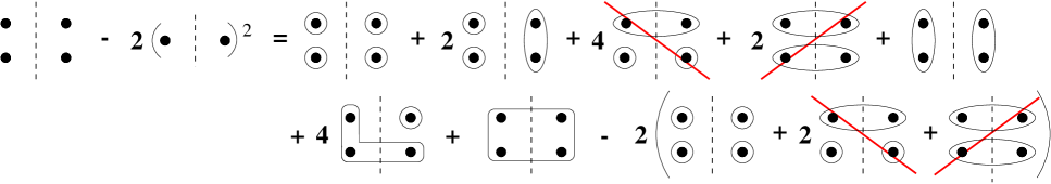
FIG. 6.: Expansion into connected parts of the cumulant of the four-particle azimuthal correlation. Dots on the left (resp. right) of the dashed line represent $e^{i\phi}$ (resp. $e^{-i\phi}$).

The diagrams in Fig. 6 stand for:

$$\left\langle e^{i(\phi_{1}+\phi_{2}-\phi_{3}-\phi_{4})}\right\rangle-2\left\langle e^{i(\phi_{1}-\phi_{3})}\right\rangle^{2}= - v_{1}^{4}+2\,v_{1}^{2}\left\langle e^{-i(\phi_{3}+\phi_{4})}\right\rangle_{c}+\left\langle e^{i(\phi_{1}+\phi_{2})}\right\rangle_{c}\left\langle e^{-i(\phi_{3}+\phi_{4})}\right\rangle_{c}$$ (A2)

$$+ 4\,v_{1}\left\langle e^{\pm i(\phi_{1}+\phi_{2}-\phi_{3})}\right\rangle_{c}+\left\langle e^{i(\phi_{1}+\phi_{2}-\phi_{3}-\phi_{4})}\right\rangle_{c}.$$ (A3)

Note that the direct two-particle correlations $\left\langle e^{i(\phi_{1}-\phi_{3})}\right\rangle_{c}$ are automatically removed. In the isotropic case, only the connected part of the correlation, i.e. $\left\langle e^{i(\phi_{1}+\phi_{2}-\phi_{3}-\phi_{4})}\right\rangle_{c}$, remains in the right-hand side of Eq. (A2).

Let us now enumerate the orders of magnitude of the different terms in the right-hand side of Eq. (A2). As stated above, all terms but the last vanish in the isotropic case: indeed, $\left\langle e^{i(\phi_{1}+\phi_{2}-\phi_{3})}\right\rangle_{c}$ and $\left\langle e^{\pm i(\phi_{1}+\phi_{2})}\right\rangle_{c}$ are not invariant under the transformation $\phi_{j}\rightarrow\phi_{j}+\alpha$, where $\alpha$ is any angle. Therefore, it seems reasonable to consider that these terms are proportional to $v_{1}$ or $v_{2}$, depending on whether a factor $e^{\pm i\alpha}$ or $e^{\pm 2i\alpha}$ appears under the previous transformation. Furthermore, since we consider here connected $k$-particle correlations, they behave like $O(1/N^{k-1})$ [see Sec. II C]. More precisely,

$$\left\langle e^{i(\phi_{1}+\phi_{2}-\phi_{3})}\right\rangle_{c}=O\left(\frac{v_{1}}{N^{2}}\right),\qquad\left\langle e^{\pm i(\phi_{1}+\phi_{2})}\right\rangle_{c}=O\left(\frac{v_{2}}{N}\right).$$ (A4)

Note that the second term in the right-hand side of Eq. (A2) is smaller than either the first or the third terms.

Finally, the order of magnitude of the right-hand side of Eq. (A1) is $v_{1}^{4}+O(v_{2}^{2}/N^{2}+1/N^{3})$. We have neglected $v_{1}^{2}/N^{2}$ since it is smaller than either $v_{1}^{4}$ or $1/N^{3}$.

2 Calculation of the cumulant $\left\langle\!\!\left\langle|Q|^{4}\right\rangle\!\!\right\rangle$

In this section, we derive the order of magnitude of the fourth order cumulant of the $|Q|^{2}$ distribution, defined by Eq. (29). From the definition of the event flow vector Eq. (22), one obtains

$$\left\langle\!\!\left\langle|Q|^{4}\right\rangle\!\!\right\rangle=\frac{1}{M^{2}}\sum_{j,k,l,m}\left(\left\langle e^{i(\phi_{j}+\phi_{k}-\phi_{l}-\phi_{m})}\right\rangle-\left\langle e^{i(\phi_{j}-\phi_{l})}\right\rangle\left\langle e^{i(\phi_{k}-\phi_{m})}\right\rangle-\left\langle e^{i(\phi_{j}-\phi_{m})}\right\rangle\left\langle e^{i(\phi_{k}-\phi_{l})}\right\rangle\right).$$ (A5)

In the above sum, one may distinguish nondiagonal terms, when all four indices are different, and diagonal terms, for which at least two indices are equal.

Nondiagonal terms correspond precisely to the cumulant of the four-particle correlation. The corresponding contribution, evaluated in Sec. A 1, must be multiplied by the combinatorial factor $M(M-1)(M-2)(M-3)\sim M^{4}$. With the factor $1/M^{2}$ in front of the sum in Eq. (A5), the contribution of nondiagonal terms to $\left\langle\!\!\left\langle|Q|^{4}\right\rangle\!\!\right\rangle$ is of order $M^{2}v_{1}^{4}+O(v_{2}^{2}+1/N)$.

We are now going to show that diagonal terms give a contribution at most of the same order as nondiagonal terms. Let us enumerate the various diagonal terms:

1. If $j=k=l=m$, each term in the sum is equal to $-1$. This is the contribution which we call “autocorrelations”. Multiplying by a combinatorial factor $M$ and by the factor $1/M^{2}$ in Eq. (A5), the corresponding contribution is exactly $-1/M$.

2. When three indices are identical while the fourth is different, i.e. in $4M(M-1)$ cases, the difference in Eq. (A5) reduces to $-\left\langle e^{i(\phi_{1}-\phi_{2})}\right\rangle$. Using Eq. (8), this contribution is of order $-4v_{1}^{2}+O(1/N)$. Although this contribution is a two-particle correlation, it is suppressed by the combinatorial factor: $v_{1}^{2}$ is much smaller than the term $M^{2}v_{1}^{4}$ which appears in the cumulant of the four-particle azimuthal correlation (see Sec. A 1). Therefore, this contribution will be negligible.

3. Let us consider the cases when the indices are equal two by two.

   • If $j=k$ and $l=m$ but $j\neq l$, which occurs $M(M-1)$ times, the difference is given by

     $$\left\langle e^{2i(\phi_{1}-\phi_{3})}\right\rangle-2\left\langle e^{i(\phi_{1}-\phi_{3})}\right\rangle^{2}=v_{2}^{2}+\left\langle e^{2i(\phi_{1}-\phi_{3})}\right\rangle_{c}-2\left(v_{1}^{2}+\left\langle e^{i(\phi_{1}-\phi_{3})}\right\rangle_{c}\right)^{2}.$$ (A6)

     The order of magnitude is then $v_{2}^{2}+O(1/N)$. Here, we have neglected terms of order $v_{1}^{2}/N$ and $1/N^{2}$, smaller than $1/N$; the term $v_{1}^{4}$ is smaller by a combinatorial factor $1/M^{2}$ than the similar contribution of nondiagonal terms. Note that the higher harmonic $v_{2}$ contributes here. We shall see below that these higher harmonics can limit the use of our method.

   • The $2M(M-1)$ cases {$j=m$ and $k=l$ but $j\neq l$} or {$j=l$ and $k=m$ but $k\neq l$} yield a contribution $-\left\langle e^{i(\phi_{1}-\phi_{3})}\right\rangle^{2}$. Its order of magnitude is $-2v_{1}^{4}+O(1/N^{2})$, negligible compared to nondiagonal terms.

4. There are two cases when three indices are different:

   • If $j=l$ or $j=m$ or $k=l$ or $k=m$, while the two remaining indices are different, the contribution is $-\left\langle e^{i(\phi_{1}-\phi_{3})}\right\rangle^{2}$, to be multiplied by a combinatorial factor $4M(M-1)(M-2)$. Thus, the order of magnitude is $M[-4v_{1}^{4}+O(1/N^{2})]$ and this contribution is suppressed by a factor $1/M$ with respect to the cumulant of the four-particle correlation.

   • If the two identical indices are either $(j,k)$ or $(l,m)$, the combinatorial factor is $2M(M-1)(M-2)$, which multiplies a term $\left\langle e^{\pm i(2\phi_{1}-\phi_{3}-\phi_{4})}\right\rangle-2\left\langle e^{i(\phi_{1}-\phi_{3})}\right\rangle^{2}$. Using Eq. (9), the three-particle correlation $\left\langle e^{i(2\phi_{1}-\phi_{3}-\phi_{4})}\right\rangle$ can be expanded as

     $$\left\langle e^{i(2\phi_{1}-\phi_{3}-\phi_{4})}\right\rangle = \left\langle e^{2i\phi_{1}}\right\rangle\left\langle e^{-i\phi_{3}}\right\rangle\left\langle e^{-i\phi_{4}}\right\rangle+\left\langle e^{i(2\phi_{1}-\phi_{3})}\right\rangle_{c}\left\langle e^{-i\phi_{4}}\right\rangle+\left\langle e^{i(2\phi_{1}-\phi_{4})}\right\rangle_{c}\left\langle e^{-i\phi_{3}}\right\rangle$$ (A8)

     $$+\left\langle e^{2i\phi_{1}}\right\rangle\left\langle e^{-i(\phi_{3}+\phi_{4})}\right\rangle_{c}+\left\langle e^{i(2\phi_{1}-\phi_{3}-\phi_{4})}\right\rangle_{c}$$

     $$= v_{2}v_{1}^{2}+O\left(\frac{v_{1}^{2}}{N}\right)+O\left(\frac{v_{2}^{2}}{N}\right)+O\left(\frac{1}{N^{3}}\right).$$ (A9)

     The second term in the difference, $-2\left\langle e^{i(\phi_{1}-\phi_{3})}\right\rangle^{2}$, gives a contribution of $-2v_{1}^{4}+O(1/N^{2})$. Finally, since terms such as $v_{1}^{4}$, $v_{1}^{2}/N$ are suppressed because of the combinatorial factor, the contribution in this case is $2Mv_{2}v_{1}^{2}+O(Mv_{2}^{2}/N)+O(M/N^{2})$.

We shall assume that the total multiplicity in the collision $N$ and the number $M$ of particles used to calculated the flow vector are large and of the same order of magnitude. Then, we find that the contribution of the diagonal terms is $-1/M+v_{2}^{2}+2Mv_{1}^{2}v_{2}+O(v_{2}^{2}+1/M)$.

All in all, when we add the contributions of diagonal and nondiagonal terms, we obtain the following result:

$$\left\langle\!\!\left\langle|Q|^{4}\right\rangle\!\!\right\rangle=-\frac{1}{M}-M^{2}v_{1}^{4}+2Mv_{1}^{2}v_{2}+v_{2}^{2}+O(v_{2}^{2})+O\left(\frac{1}{M}\right).$$ (A10)

The first term in the right-hand side coresponds to autocorrelations, the last two terms are due to nonflow correlations, and the three remaining terms arise from flow. One would like $-M^{2}v_{1}^{4}$ to be the dominant flow term. However, higher harmonics, i.e. $v_{2}$, also contribute. If $v_{2}$ is large enough, it may even reverse the sign of the contribution of flow to $\left\langle\!\!\left\langle|Q|^{4}\right\rangle\!\!\right\rangle$. This does not happen provided $v_{2}$ lies in the following interval :

$$-Mv_{1}^{2}(\sqrt{2}+1)<v_{2}<Mv_{1}^{2}(\sqrt{2}-1).$$ (A11)

We have checked these bounds with our Monte-Carlo simulation, see Sec. V C.

B A generating equation for the integrated flow

In this Appendix, we first construct the cumulants of the distribution of $|Q|$, which we note $\left\langle\!\!\left\langle|Q|^{2k}\right\rangle\!\!\right\rangle$, as a function of the measured moments $\left\langle|Q|^{2k}\right\rangle$ (Secs. B 1 and B 2). Then, we relate the cumulants to the integrated flow $\left\langle Q\right\rangle$ (Sec. B 3), and show how to remove autocorrelations at all orders (Sec. B 4).

1 Cluster decomposition of the moments

We have shown in Sec. II C how the $k$-particle momentum distribution can be decomposed, in a coordinate frame where the reaction plane is fixed, into a sum of terms involving lower order distributions ($k^{\prime}$ particles with $k^{\prime}<k$), plus a “connected” term of relative order $1/N^{k-1}$. This decomposition also applies to the moments of the distribution of the event flow vector $Q$ defined by Eq. (22). As pointed out in Sec. III B, moments of order $k$ involve $k$-particle azimuthal correlations. This allows us to write a series of equations similar to Eqs. (6) and (9):

$$\left\langle Q\right\rangle = \left\langle Q\right\rangle_{c}$$ (B2)

$$\left\langle Q^{2}\right\rangle = \left\langle Q\right\rangle_{c}^{2}+\left\langle Q^{2}\right\rangle_{c}$$ (B3)

$$\left\langle QQ^{*}\right\rangle = \left\langle Q\right\rangle_{c}\left\langle Q^{*}\right\rangle_{c}+\left\langle QQ^{*}\right\rangle_{c}$$ (B4)

$$\left\langle Q^{3}\right\rangle = \left\langle Q\right\rangle_{c}^{3}+3\left\langle Q\right\rangle_{c}\left\langle Q^{2}\right\rangle_{c}+\left\langle Q^{3}\right\rangle_{c}$$ (B5)

$$\left\langle Q^{2}Q^{*}\right\rangle = \left\langle Q\right\rangle_{c}^{2}\left\langle Q^{*}\right\rangle_{c}+2\left\langle Q\right\rangle_{c}\left\langle QQ^{*}\right\rangle_{c}+\left\langle Q^{2}\right\rangle_{c}\left\langle Q^{*}\right\rangle_{c}+\left\langle Q^{2}Q^{*}\right\rangle_{c},{\rm\ etc.}$$ (B6)

In these equations, the subscript $c$ denotes “connected” moments. The connected moment of order $k$ is of magnitude $M^{1-k/2}$: a factor $M^{1-k}$ comes from the fact that it involves direct $k$-particle correlations (see Sec. II C), and a factor $M^{k/2}$ from the scaling of $Q$ with the number of particles like $\sqrt{M}$, see Eq. (22).

The expansion of a given moment $\left\langle Q^{k}Q^{*l}\right\rangle$ in connected parts can be represented graphically by the expansion of a $(k+l)$-point diagram into connected diagrams. This is similar to the decomposition of the $k$-particle distribution in Figs. 1 and 2. To be more specific, the decomposition of $\left\langle Q^{k}Q^{*l}\right\rangle$ is represented by drawing $k$ dots of one type corresponding to powers of $Q$ and $l$ dots of another type corresponding to powers of $Q^{*}$. One then takes all possible partitions of this set of $k+l$ points. To each subset of points one associates the corresponding connected moment. The contribution of a given partition is the product of the contributions of each subset. Finally, $\left\langle Q^{k}Q^{*l}\right\rangle$ is the sum of the contributions of all partitions. Figure 7 represents, as an example, the decomposition of $\left\langle Q^{2}Q^{*}\right\rangle$.

FIG. 7.: Decomposition of $\left\langle Q^{2}Q^{*}\right\rangle$ in connected parts, see Eq. (B6). Dots on the left of the dashed line represent factors of $Q$ while dots on the right represent factors of $Q^{*}$. Circled subsets correspond to connected moments.

The connected moments can be expressed as a function of the moments by inverting Eqs. (B 1) order by order. However, this procedure is very tedious. An elegant and compact way to express moments of arbitrary order in terms of the connected parts, and to invert these relations, consists in using generating functions. The generating function of the moments is a function of the complex variable $z$ which is defined as

$${\cal G}_{0}(z)=\left\langle e^{z^{*}Q+zQ^{*}}\right\rangle=\sum_{k,l}{z^{*k}z^{l}\over k!\,l!}\left\langle Q^{k}Q^{*l}\right\rangle,$$ (B7)

where $k$ and $l$ go from $0$ to $+\infty$, and the brackets denote an average over many events. It is well known in graph theory that the generating function of connected diagrams is the logarithm of the generating function of all diagrams [35]. Therefore, the generating function of the connected moments is the logarithm of the generating function of the moments [20]:

$$\sum_{k,l}{z^{*k}z^{l}\over k!\,l!}\left\langle Q^{k}Q^{*l}\right\rangle_{c}=\ln{\cal G}_{0}(z).$$ (B8)

The normalization coefficient $1/k!\,l!$ has been chosen such that $\left\langle Q^{k}Q^{*l}\right\rangle_{c}$ appears with a unit coefficient in the expansion of $\left\langle Q^{k}Q^{*l}\right\rangle$, as in Eq. (B 1). Expanding Eqs. (B7) and (B8) to order $z^{*2}z$, one finds for instance

$$\left\langle Q^{2}Q^{*}\right\rangle_{c} = \left\langle Q^{2}Q^{*}\right\rangle-\left\langle Q^{2}\right\rangle\left\langle Q^{*}\right\rangle-2\left\langle Q\right\rangle\left\langle QQ^{*}\right\rangle+2\left\langle Q\right\rangle^{2}\left\langle Q^{*}\right\rangle,$$ (B9)

which can be checked by inverting Eqs. (B 1) order by order. Note that we are working in a coordinate system where the reaction plane correponds to the $x$-axis, and is unknown. In this coordinate system, the generating function (B7) is not a measurable quantity.

2 Isotropic source

We now consider specifically an isotropic source, i.e. without flow. In that case, the moment $\left\langle Q^{k}Q^{*l}\right\rangle$ vanishes if $k\not=l$. The connected parts $\left\langle Q^{k}Q^{*l}\right\rangle_{c}$ enjoy the same property. Therefore, in the diagrammatic expansion, one only retains terms containing as many powers of $Q$ as of $Q^{*}$, i.e. as many dots on the left as on the right. The quantity represented in Fig. 7 does not satisfy this property, and therefore it vanishes. A decomposition with nonvanishing terms is represented in Fig. 3.

Keeping only the terms $k=l$, the generating function (B7) becomes

$${\cal G}_{0}(z)=\sum_{k=0}^{\infty}\frac{|z|^{2k}}{(k!)^{2}}\left\langle|Q|^{2k}\right\rangle=\left\langle I_{0}(2|zQ|)\right\rangle,$$ (B10)

where $I_{0}$ is the modified Bessel function of order $0$. Note that now the generating function ${\cal G}_{0}$ itself is isotropic, since ${\cal G}_{0}(z)={\cal G}_{0}(ze^{i\alpha})$. The consequence is that it can be evaluated in the laboratory coordinate system rather than in the coordinate system associated with the reaction plane: it thus becomes a measurable quantity. We define the cumulants through

$$\sum_{k=1}^{\infty}\frac{|z|^{2k}}{(k!)^{2}}\left\langle\!\!\left\langle|Q|^{2k}\right\rangle\!\!\right\rangle\equiv\ln{\cal G}_{0}(z)=\ln\left\langle I_{0}(2|zQ|)\right\rangle.$$ (B11)

They coincide with the connected moments $\left\langle|Q|^{2k}\right\rangle_{c}$ defined in Eq. (B8) if the source is isotropic. Note that for an isotropic system, the raw moment $\left\langle|Q|^{2k}\right\rangle$ is of order unity, as noted in Sec. III B. The corresponding cumulant $\left\langle\!\!\left\langle|Q|^{2k}\right\rangle\!\!\right\rangle$ is of order $M^{1-k}$. Eq. (B11) corresponds to Eq.(32), where we have set $x=|z|$.

3 Flow

Let us now calculate the cumulants in the case of collisions with flow. Neglecting for simplicity nonflow correlations between particles, we can write $\left\langle Q^{k}Q^{*l}\right\rangle=\left\langle Q\right\rangle^{k}\left\langle Q^{*}\right\rangle^{l}=\left\langle Q\right\rangle^{k+l}$. The generating function (B7) thus becomes

$${\cal G}_{0}(z)=e^{(z+z^{*})\left\langle Q\right\rangle}.$$ (B12)

Now, we want to compare with the experimental value of ${\cal G}_{0}(z)$, which is measured in the laboratory coordinate system where the azimuth of the reaction plane $\phi_{R}\neq 0$. The generating function in this coordinate system is deduced from Eq. (B12) by the substitution $z\to ze^{i\phi_{R}}$. Averaging the new expression over all possible $\phi_{R}$, under the assumption that the distribution of $\phi_{R}$ is uniform, one obtains:

$${\cal G}_{0}(z)=\frac{1}{2\pi}\displaystyle\int_{0}^{2\pi}\!e^{(ze^{i\phi_{R}}+z^{*}e^{-i\phi_{R}})\left\langle Q\right\rangle}\,{\rm d}\phi_{R}=I_{0}(2|z|\left\langle Q\right\rangle).$$ (B13)

Gathering the results obtained in Eqs. (B11) and (B13), we obtain:

$$\sum_{k=1}^{\infty}\frac{|z|^{2k}}{(k!)^{2}}\left\langle\!\!\left\langle|Q|^{2k}\right\rangle\!\!\right\rangle=\ln{\cal G}_{0}(z)=\ln I_{0}(2|z|\left\langle Q\right\rangle).$$ (B14)

Expanding Eq. (B14) to order $|z|^{2k}$, one obtains an equation relating $\left\langle Q\right\rangle^{2k}$ to the cumulant $\left\langle\!\!\left\langle|Q|^{2k}\right\rangle\!\!\right\rangle$. However, when writing Eq. (B12), we have neglected direct $2k$-particle correlations and autocorrelations. As explained in Sec. B 1, both give a contribution of magnitude $M^{1-k}$ to the cumulant $\left\langle\!\!\left\langle|Q|^{2k}\right\rangle\!\!\right\rangle$. Thus, Eq. (B14) at order $|z|^{2k}$ is valid up to a corrrection of order $M^{1-k}$.

4 Removing autocorrelations

Equation (B14) can be somewhat refined. In the case of a $Q$ vector defined with unit weights, as in Eq. (22), autocorrelations can be calculated and subtracted explicitly, which is the purpose of this section.

This calculation has already been done in Sec. III for the lowest orders $k=1$ and $k=2$: we have seen in Eq. (25) that diagonal terms give a contribution 1 in the expansion of $\left\langle|Q|^{2}\right\rangle$. In this paper, we refer to these diagonal terms as “autocorrelations”. Similarly, they give a contribution $-1/M$ to the fourth order cumulant $\left\langle\!\!\left\langle|Q|^{4}\right\rangle\!\!\right\rangle$, see Eq. (34) and Appendix A.

To calculate the contribution of autocorrelations to the cumulant at an arbitrary order, we once again make use of the generating function ${\cal G}_{0}(z)$, Eq. (B7). Neglecting correlations for simplicity, the contributions of the $M$ particles to ${\cal G}_{0}(z)$ factorize, leading to

$${\cal G}_{0}(z)=\left\langle e^{(2x\cos\phi+2y\sin\phi)/\sqrt{M}}\right\rangle_{\phi}^{M},$$ (B15)

where we have set $z=x+iy$, and the brackets here denote an average over $\phi$. Assuming for simplicity that the $\phi$ distribution is isotropic, one obtains

$${\cal G}_{0}(z)=\left[I_{0}\!\left({2|z|\over\sqrt{M}}\right)\right]^{M}.$$ (B16)

This is the expression of the generating function if there are only autocorrelations (no direct correlations, no flow). If there is flow, we assume that autocorrelations and flow give additive contributions to the cumulants, which yields instead of Eq. (B14):

$$\sum_{k=0}^{\infty}\frac{|z|^{2k}}{(k!)^{2}}\left\langle\!\!\left\langle|Q|^{2k}\right\rangle\!\!\right\rangle=\ln{\cal G}_{0}(z)=\ln I_{0}(2|z|\left\langle Q\right\rangle)+M\ln I_{0}\!\left({2|z|\over\sqrt{M}}\right).$$ (B17)

This formula is equivalent to Eq. (35), which we use in Sec. III B. It removes exactly all autocorrelations when the event flow vector $Q$ is defined with unit weights, as in Eq. (22).

C A generating equation for differential flow

In this appendix, we follow closely the same procedure as in Appendix B, applied to differential flow. In Secs. C 1 and C 2, we first construct the relevant cumulants $\left\langle\!\!\left\langle|Q|^{2k}Q^{*l}e^{im\psi}\right\rangle\!\!\right\rangle$, as a function of the measured moments $\left\langle Q^{k}Q^{*l}e^{im\psi}\right\rangle$. Here, $\psi$ denotes the azimuthal angle of the particle under study (which we call a proton), and $m$ the order of the harmonic measured for this particle. Then, we relate the cumulants to the integrated flow $v^{\prime}_{m}$ (Sec. C 3), and show how to remove autocorrelations (Sec. C 4).

1 Cluster decomposition

A quantity such as $\left\langle Q^{k}Q^{*l}e^{im\psi}\right\rangle$ involves correlations between $k+l+1$ particles: $k+l$ “pions” (according to the terminology introduced in Sec. IV) and a proton. This quantity can therefore be decomposed, in the coordinate system where the reaction plane is fixed, into a sum of terms involving lower order correlations, plus a connected term of relative order $1/N^{k+l}$. For instance, we can write

$$\left\langle e^{im\psi}\right\rangle = \left\langle e^{im\psi}\right\rangle_{c}$$ (C2)

$$\left\langle Qe^{im\psi}\right\rangle = \left\langle Q\right\rangle_{c}\left\langle e^{im\psi}\right\rangle_{c}+\left\langle Qe^{im\psi}\right\rangle_{c}$$ (C3)

$$\left\langle QQ^{*}e^{im\psi}\right\rangle = \left\langle Q\right\rangle_{c}\left\langle Q^{*}\right\rangle_{c}\left\langle e^{im\psi}\right\rangle_{c}+\left\langle QQ^{*}\right\rangle_{c}\left\langle e^{im\psi}\right\rangle_{c}+\left\langle Q\right\rangle_{c}\left\langle Q^{*}e^{im\psi}\right\rangle_{c}+\left\langle Q^{*}\right\rangle_{c}\left\langle Qe^{im\psi}\right\rangle_{c}+\left\langle QQ^{*}e^{im\psi}\right\rangle_{c},$$ (C4)

where, in the third equation, the last term is of order $1/N^{2}$ relative to the first one. Such decompositions can be represented diagrammatically, in a way similar to the decomposition of $\left\langle Q^{k}Q^{*l}\right\rangle$ in Appendix B. We choose to represent the proton by $m$ crosses on the left, for reasons which will become clear below, when we consider the specific case of an isotropic source. For instance, Eq. (C4) can be represented diagrammatically by Fig. 8.

FIG. 8.: Decomposition of $\left\langle QQ^{*}e^{2i\psi}\right\rangle$ in connected parts, see Eq. (C4). As in Fig. 7, the dot on the left (resp. right) of the dashed line stands for $Q$ (resp. $Q^{*}$). The linked crosses represent the proton, the number of crosses being chosen equal to the harmonic under study, here $m=2$. Circled subsets (connected diagrams) correspond to connected moments.

In order to express in a compact way the relations between the moments $\left\langle Q^{k}Q^{*l}e^{im\psi}\right\rangle$ and the corresponding connected moments $\left\langle Q^{k}Q^{*l}e^{im\psi}\right\rangle_{c}$, we introduce the following generating function

$${\cal G}_{m}(z)=\left\langle e^{z^{*}Q+zQ^{*}}e^{im\psi}\right\rangle=\sum_{k,l}{z^{*k}z^{l}\over k!\,l!}\left\langle Q^{k}Q^{*l}e^{im\psi}\right\rangle,$$ (C5)

Expanding ${\cal G}_{m}(z)$ to order $z^{*k}z^{l}$, one obtains all the moments $\left\langle Q^{k}Q^{*l}e^{im\psi}\right\rangle$. In order to obtain the generating function of the connected moments, we note that each diagram in Fig. 8 can be written as the product of a connected diagram containing the crosses, i.e. the proton, times an arbitrary diagram (not necessarily connected) involving only pions, which corresponds to the terms $\left\langle Q^{k}Q^{*l}\right\rangle$ considered in Appendix B. For instance, using Eqs. (B2) and (B4), one can rewrite Eq. (C4) as

$$\left\langle QQ^{*}e^{im\psi}\right\rangle=\left\langle QQ^{*}\right\rangle\left\langle e^{im\psi}\right\rangle_{c}+\left\langle Q\right\rangle\left\langle Q^{*}e^{im\psi}\right\rangle_{c}+\left\langle Q^{*}\right\rangle\left\langle Qe^{im\psi}\right\rangle_{c}+\left\langle QQ^{*}e^{im\psi}\right\rangle_{c}.$$ (C6)

Therefore, the generating function of the diagrams with pions and protons $\left\langle e^{z^{*}Q+zQ^{*}+im\psi}\right\rangle$ is the product of the generating function of graphs with only pions, i.e. ${\cal G}_{0}(z)$ defined in Eq. (B7), by the generating function of connected graphs with pions and protons. This latter is therefore:

$${\cal C}_{m}(z)=\sum_{k,l}{z^{*k}z^{l}\over k!\,l!}\left\langle Q^{k}Q^{*l}e^{im\psi}\right\rangle_{c}\equiv{{\cal G}_{m}(z)\over{\cal G}_{0}(z)}=\frac{\left\langle e^{z^{*}Q+zQ^{*}+im\psi}\right\rangle}{\left\langle e^{z^{*}Q+zQ^{*}}\right\rangle}$$ (C7)

As in Eq. (B8), the normalization coefficient $1/k!\,l!$ has been chosen so that $\left\langle Q^{k}Q^{*l}e^{im\psi}\right\rangle_{c}$ appears with a unit coefficient in the expansion of $\left\langle Q^{k}Q^{*l}e^{im\psi}\right\rangle$.

2 Isotropic source

We now consider the particular case of an isotropic source, without flow. Then the moment $\left\langle Q^{k}Q^{*l}e^{im\psi}\right\rangle$ vanishes when $k+m\neq l$, and so do the corresponding connected parts. This is the reason why we chose to represent the proton with $m$ crosses: in the isotropic case, only diagrams with the same number of points (crosses and dots) on each side of the dashed line do not vanish.

Expanding the generating function (C5) and keeping only the nonvanishing terms, one finds

$${\cal G}_{m}(z) = \sum_{k=0}^{\infty}\frac{|z|^{2k}z^{m}}{k!\,(k+m)!}\left\langle|Q|^{2k}{Q^{*}}^{m}e^{im\psi}\right\rangle$$ (C8)

$$= \left\langle I_{m}(2|zQ|)\left(\frac{zQ^{*}}{|zQ|}\right)^{m}e^{im\psi}\right\rangle,$$ (C9)

where $I_{m}$ is the modified Bessel function of order $m$.

We define the cumulants $\left\langle\!\!\left\langle|Q|^{2k}{Q^{*}}^{m}e^{im\psi}\right\rangle\!\!\right\rangle$ so that they coincide with the connected moments in Eq. (C7) when the source is isotropic. Using Eq. (B10), this gives

$${\cal C}_{m}(z) = \sum_{k=0}^{\infty}\frac{|z|^{2k}z^{m}}{k!\,(k+m)!}\left\langle\!\!\left\langle|Q|^{2k}{Q^{*}}^{m}e^{im\psi}\right\rangle\!\!\right\rangle$$ (C10)

$$\equiv \frac{\left\langle I_{m}(2|zQ|)\left(\frac{zQ^{*}}{|zQ|}\right)^{m}e^{im\psi}\right\rangle}{\left\langle I_{0}(2|zQ|)\right\rangle}.$$ (C11)

This equation is equivalent to Eq. (80), setting $x=|z|$.

3 Flow

Finally, we turn to the more general case of collisions with flow. Neglecting for simplicity nonflow correlations between particles, the generating function (C5) becomes

$${\cal G}_{m}(z)=e^{(z+z^{*})\left\langle Q\right\rangle}v^{\prime}_{m}.$$ (C12)

As explained in Sec. B 3, this quantity is measured in the laboratory coordinate system, therefore one must replace $z$ by $ze^{i\phi_{R}}$ and average the new expression over all possible $\phi_{R}$. That yields

$${\cal G}_{m}(z) = v^{\prime}_{m}\displaystyle\int_{0}^{2\pi}\!e^{(ze^{i\phi_{R}}+z^{*}e^{-i\phi_{R}})\left\langle Q\right\rangle}e^{im\phi_{R}}\,{{\rm d}\phi_{R}\over 2\pi}$$ (C13)

$$= I_{m}(2|z|\left\langle Q\right\rangle)\,\left(\frac{z}{|z|}\right)^{m}v^{\prime}_{m}.$$ (C14)

Using Eq. (B13), the generating function of cumulants (C7) takes the form

$${\cal C}_{m}(z)=\frac{I_{m}(2|z|\left\langle Q\right\rangle)}{I_{0}(2|z|\left\langle Q\right\rangle)}\,\left(\frac{z}{|z|}\right)^{m}v^{\prime}_{m}.$$ (C15)

Gathering Eqs. (C11) and (C15), we obtain

$$\sum_{k=0}^{\infty}\frac{|z|^{2k}z^{m}}{k!\,(k+m)!}\left\langle\!\!\left\langle|Q|^{2k}{Q^{*}}^{m}e^{im\psi}\right\rangle\!\!\right\rangle={\cal C}_{m}(z)=\frac{I_{m}(2|z|\left\langle Q\right\rangle)}{I_{0}(2|z|\left\langle Q\right\rangle)}\,\left(\frac{z}{|z|}\right)^{m}v^{\prime}_{m}.$$ (C16)

Expanding this equation to order $|z|^{2k}z^{m}$, one obtains a proportionality relation between the cumulant $\left\langle\!\!\left\langle|Q|^{2k}{Q^{*}}^{m}e^{im\psi}\right\rangle\!\!\right\rangle$ and $\left\langle Q\right\rangle^{2k+m}v^{\prime}_{m}$. Having measured independently the integrated flow $\left\langle Q\right\rangle$, one thus obtains the differential flow $v^{\prime}_{m}$ from the cumulant. As discussed in Sec. IV, the corresponding error from nonflow correlations is of order $(\left\langle Q\right\rangle\sqrt{M})^{-k-(m/2)}$.

4 Removing autocorrelations

In the case when the “proton” is included in the construction of the event flow vector $Q_{n}$, i.e. if $\psi$ is one of the angles $\phi_{j}$ in Eq. (22), the resulting autocorrelations can be removed at the level of the generating function ${\cal C}_{m}(z)$ in Eq. (C11): this subtraction is similar to that performed in Sec. B 4 for the integrated flow.

Neglecting correlations for simplicity, the generating function of the cumulants, defined by Eq. (C7), becomes

$${\cal C}_{m}(z)={\left\langle e^{(2x\cos\psi+2y\sin\psi+im\psi)/\sqrt{M}}\right\rangle_{\psi}\over\left\langle e^{(2x\cos\psi+2y\sin\psi)/\sqrt{M}}\right\rangle_{\psi}},$$ (C17)

where we have set $z=x+iy$, and the brackets denote an average over $\psi$. Assuming for simplicity that the $\psi$ distribution is isotropic, one obtains

$${\cal C}_{m}(z)={I_{m}\left({2|z|/\sqrt{M}}\right)\over I_{0}\left({2|z|/\sqrt{M}}\right)}\left({z\over|z|}\right)^{m}.$$ (C18)

This is the value of the generating function if there are only autocorrelations. If there is flow in addition, we assume that the contributions of autocorrelations and flow are additive. Equation (C16) is then replaced by

$$\sum_{k=0}^{\infty}\frac{|z|^{2k}z^{m}}{k!\,(k+m)!}\left\langle\!\!\left\langle|Q|^{2k}{Q^{*}}^{m}e^{im\psi}\right\rangle\!\!\right\rangle=\left(\frac{I_{m}(2|z|\left\langle Q\right\rangle)}{I_{0}(2|z|\left\langle Q\right\rangle)}v^{\prime}_{m}+{I_{m}\left({2|z|/\sqrt{M}}\right)\over I_{0}\left({2|z|/\sqrt{M}}\right)}\right)\,\left(\frac{z}{|z|}\right)^{m}.$$ (C19)

This equation is equivalent to Eq. (81), setting $x=|z|$. This formula removes exactly all autocorrelations when the vector $Q_{n}$ is defined with unit weights.

D Interpolation formulas

In this Appendix, we give interpolation methods to calculate numerically the cumulants from their generating functions.

1 Integrated flow

The cumulants used for the measurement of the integrated flow are defined by Eq. (99). In order to compute numerically the cumulants $\langle\!\langle|Q^{2k^{\prime}}|\rangle\!\rangle$ for $k^{\prime}=1\dots k$ from the generating function, one can for instance tabulate the generating function at the following points:

$$G_{p,q}\equiv\log{\cal G}_{0}\left(r_{0}\sqrt{p}\,\cos{2\,q\,\pi\over q_{\rm max}},r_{0}\sqrt{p}\,\sin{2\,q\,\pi\over q_{\rm max}}\right)$$ (D1)

for $p=1,\dots,k$ and $q=0,\dots,q_{\rm max}-1$. In this equation, $r_{0}$ is a real number which should be chosen small enough for the series expansion to converge rapidly, typically $r_{0}\sim 0.1$, and $q_{\rm max}$ is the number of angles at which the generating function is evaluated, which should satisfy the condition $q_{\rm max}>2k$.

One then averages over the angle, thereby eliminating nonisotropic terms up to order $|z|^{2k}$:

$$G_{p}\equiv{1\over q_{\rm max}}\sum_{q=0}^{q_{\rm max}-1}G_{p,q}.$$ (D2)

Then, the $G_{p}$, with $p=1,\dots,k$, are related to the cumulants $\langle\!\langle|\bar{Q}|^{2k^{\prime}}\rangle\!\rangle$ with $k^{\prime}=1,\dots,k$ by the following linear system of equations:

$$G_{p}=\sum_{k^{\prime}=1}^{k}\left\langle\!\!\left\langle|\bar{Q}|^{2k^{\prime}}\right\rangle\!\!\right\rangle{r_{0}^{2k^{\prime}}\over(k^{\prime}!)^{2}}\,p^{k^{\prime}}\quad 1\leq p\leq k.$$ (D3)

For practical purposes, it is enough to take $k=3$, as explained in Sec. III D. In this case, the solution of the above system reads

$$\left\langle\!\!\left\langle|\bar{Q}|^{2}\right\rangle\!\!\right\rangle = {1\over r_{0}^{2}}\,\left(3\,G_{1}-{3\over 2}G_{2}+{1\over 3}G_{3}\right),$$ (D4)

$$\left\langle\!\!\left\langle|\bar{Q}|^{4}\right\rangle\!\!\right\rangle = {2\over r_{0}^{4}}\,\left(-5\,G_{1}+4\,G_{2}-\,G_{3}\right),$$ (D5)

$$\left\langle\!\!\left\langle|\bar{Q}|^{6}\right\rangle\!\!\right\rangle = {6\over r_{0}^{6}}\,\left(3\,G_{1}-3\,G_{2}+G_{3}\right).$$ (D6)

2 Differential flow

The cumulants used for the measurement of the harmonic $v^{\prime}_{m}$ are defined from the generating function by Eq. (109). In order to compute numerically the cumulants $\langle\!\langle|Q|^{2k^{\prime}}Q^{*m}e^{im\psi}\rangle\!\rangle$ for $k^{\prime}=0,\dots,k$, from the generating function, we first tabulate the real and imaginary parts of the generating function, defined by Eq. (107), at the following points:

$$X_{p,q}\equiv{\Re}\left[{\cal C}_{m}\!\left(r_{0}\sqrt{p}\,\cos\frac{2\,q\,\pi}{q_{\rm max}},r_{0}\sqrt{p}\,\sin\frac{2\,q\,\pi}{q_{\rm max}}\right)\right]$$ (D7)

$$Y_{p.q}\equiv{\Im}\left[{\cal C}_{m}\!\left(r_{0}\sqrt{p}\,\cos\frac{2\,q\,\pi}{q_{\rm max}},r_{0}\sqrt{p}\,\sin\frac{2\,q\,\pi}{q_{\rm max}}\right)\right]$$ (D8)

for $p=1,\dots,k+1$ and $q=0,\dots,q_{\rm max}-1$. The number of angles $q_{\rm max}$ must satisfy the condition $q_{\rm max}>2(k+m)$, as we see below.

One then multiplies ${\cal C}_{m}(z)$ by $z^{*m}$, takes the real part and averages over azimuthal angles. Provided $q_{\rm max}$ is large enough, one thus eliminates all nonisotropic terms up to order $z^{*k}z^{k+m}$ in the generating function:

$$C_{p}\equiv{\left(r_{0}\sqrt{p}\right)^{m}\over q_{\rm max}}\sum_{q=0}^{q_{\rm max}-1}\left[\cos\left(m\frac{2\,q\,\pi}{q_{\rm max}}\right)\,X_{p,q}+\sin\left(m\frac{2\,q\,\pi}{q_{\rm max}}\right)\,Y_{p,q}\right].$$ (D9)

Then, the values of $C_{p}$ for $p=1,\dots k+1$ are related to the cumulants $\langle\!\langle|Q|^{2k^{\prime}}Q^{*m}e^{im\psi}\rangle\!\rangle$ for $k^{\prime}=0,\dots,k$ by the following linear system of equations:

$$C_{p}=\sum_{k^{\prime}=0}^{k}\left\langle\!\!\left\langle|\bar{Q}|^{2k^{\prime}}\bar{Q}^{*m}e^{im\bar{\psi}}\right\rangle\!\!\right\rangle{r_{0}^{2(k^{\prime}+m)}p^{k^{\prime}+m}\over k^{\prime}!(k^{\prime}+m)!},\quad 1\leq p\leq k+1.$$ (D10)

Taking $k=1$ is sufficient for most purposes, as shown in Sec. IV C. For $m=1$, the solution of this system is

$$\left\langle\!\!\left\langle\bar{Q}^{*}e^{i\bar{\psi}}\right\rangle\!\!\right\rangle = {1\over r_{0}^{2}}\left(2\,C_{1}-{1\over 2}\,C_{2}\right),$$ (D11)

$$\left\langle\!\!\left\langle|\bar{Q}|^{2}\bar{Q}^{*}e^{i\bar{\psi}}\right\rangle\!\!\right\rangle = {1\over r_{0}^{4}}\left(-2\,C_{1}+C_{2}\right),$$ (D12)

while for $m=2$,

$$\left\langle\!\!\left\langle\bar{Q}^{*2}e^{2i\bar{\psi}}\right\rangle\!\!\right\rangle = {1\over r_{0}^{4}}\left(4\,C_{1}-{1\over 2}\,C_{2}\right),$$ (D13)

$$\left\langle\!\!\left\langle|\bar{Q}|^{2}\bar{Q}^{*2}e^{2i\bar{\psi}}\right\rangle\!\!\right\rangle = {1\over r_{0}^{6}}\left(-6\,C_{1}+{3\over 2}\,C_{2}\right).$$ (D14)

REFERENCES

- [1] For a review, see J.-Y. Ollitrault, Nucl. Phys. A638, 195c (1998).
- [2] P. Danielewicz and G. Odyniec, Phys. Lett. 157B, 146 (1985).
- [3] P. M. Dinh, N. Borghini, and J.-Y. Ollitrault, Phys. Lett. B477, 51 (2000).
- [4] N. Borghini, P. M. Dinh, and J.-Y. Ollitrault, Phys. Rev. C62, 034902 (2000).
- [5] P. Danielewicz et al., Phys. Rev. C38, 120 (1988).
- [6] H. Sorge, Phys. Rev. Lett. 82 (1999) 2048.
- [7] S. A. Voloshin and A. M. Poskanzer, Phys. Lett. B474 (2000) 27.
- [8] L. V. Bravina, A. Faessler, C. Fuchs, and E. E. Zabrodin, Phys. Rev. C61 (2000) 064902.
- [9] A. M. Poskanzer and S. A. Voloshin, Phys. Rev. C58, 1671 (1998).
- [10] M. M. Aggarwal et al., WA93 Collaboration, Phys. Lett. B403 (1997) 390; W.H. van Heeringen, Ph.D. Thesis, ISBN 90-393-1325-3, Universiteit Utrecht (1996).
- [11] K. H. Ackermann et al. (STAR Collaboration), preprint nucl-ex/0009011.
- [12] J. Jiang et al., Phys. Rev. Lett. 68, 2739 (1992).
- [13] S. A. Voloshin and Y. Zhang, Z. Phys. C70, 665 (1996).
- [14] J. Barrette et al. (E877 Collaboration), Phys. Rev. Lett. 73, 2532 (1994).
- [15] B. Lenkeit for the CERES Collaboration, Nucl. Phys. A661, 23c (1999).
- [16] A. M. Poskanzer and S. A. Voloshin, unpublished.
- [17] H. Appelshäuser et al. (NA49 Collaboration), Phys. Rev. Lett. 80, 4136 (1998).
- [18] J. Barrette et al. (E877 Collaboration), Phys. Rev. C55, 1420 (1997).
- [19] T. L. Hill, Statistical Mechanics, (McGraw-Hill, NY, 1956), chapter 5.
- [20] N. G. van Kampen, Stochastic processes in physics and chemistry (North-Holland, Amsterdam, 1981).
- [21] P. Carruthers and I. Sarcevic, Phys. Rev. Lett. 63, 1562 (1989).
- [22] A. Giovannini and G. Veneziano, Nucl. Phys. B130, 61 (1977).
- [23] H. C. Eggers, P. Lipa, P. Carruthers, and B. Buschbeck, Phys. Lett. B301, 298 (1993).
- [24] J.-Y. Ollitrault, Phys. Rev. D46, 229 (1992); Phys. Rev. D48, 1132 (1993).
- [25] W. K. Wilson, R. Lacey, C. A. Ogilvie, and G. D. Westfall, Phys. Rev. C45, 738 (1992).
- [26] J.-Y. Ollitrault, Nucl. Phys. A590, 561c (1995).
- [27] P. Saturnini (NA50 Collaboration), Nucl. Phys. A661, 345c (1999).
- [28] A. M. Poskanzer and S. A. Voloshin (NA49 Collaboration) Nucl. Phys. A661, 341c (1999).
- [29] P. Danielewicz and M. Gyulassy, Phys. Lett. 129B, 283 (1983).
- [30] H. Gustafsson et al., Phys. Rev. Lett. 52, 1590 (1984).
- [31] K. G. R. Doss et al., Phys. Rev. Lett. 59, 2720 (1987).
- [32] J.-Y. Ollitrault, “A method of reconstructing azimuthal distributions in heavy ion collisions,” in XXV International Symposium on Multiparticle Dynamics, Stara Lesna, Slovakia, 11-16 september 1995, Bruncko D., Sandor L., Urban J. eds., (World Scientific, 1996), pp. 290-296; J.-Y. Ollitrault, Los Alamos preprint nucl-ex/9711003, unpublished.
- [33] J. Barrette et al. (E877 Collaboration), Phys. Rev. C56, 3254 (1997); Phys. Rev. C59, 884 (1999).
- [34] N. Borghini, P. M. Dinh, and J.-Y. Ollitrault, in preparation.
- [35] C. Domb and M. S. Green Eds., Phase transitions and critical phenomena, vol.3: Series expansions for lattice models (Academic Press, New York, 1974).