Coupling of Dipole Mode to -unstable Quadrupole Oscillations
Abstract
The coupling of the high-lying dipole mode to the low-lying quadrupole modes for the case of deformed -unstable nuclei is studied. Results from the geometrical model are compared to those obtained within the dipole boson model. Consistent results are obtained in both models. The dipole boson model is treated within the intrinsic frame, with subsequent projection onto the laboratory frame. As an application, calculations of photonuclear cross-sections in -unstable nuclei are presented.
PACS numbers: 21.60.Ev, 21.60.Fw, 21.10.Re
I Introduction
Low-lying quadrupole oscillations in nuclei have been studied extensively with all kinds of nuclear structure models. Among the more popular are the geometrical model[1] and the interacting boson model (IBM)[2]. Although rather different in their microscopic interpretation and formulation, both of them have been extremely successful in describing low-lying energy levels associated to quadrupole oscillations. In three different situations both models provide analytical results that can be identified in the geometrical model as those corresponding to spherical[1], well quadrupole deformed [1] and deformed -unstable shapes[3]. The corresponding situations occur in IBM for the U(5)[4], SU(3)[5] and O(6)[6] limits respectively. Connection between both models has been established by exploring the geometrical content of the IBM by using coherent states [7, 8, 9].
High-lying dipole states are studied in the context of the geometrical model by using the dynamic collective model within the hydrodynamical approach[10, 11]. In the IBM context these states can be studied with the so called dipole boson model [12, 13, 14, 15], which includes a dipole boson into the usual IBM space (quadrupole and bosons). The connection between both approaches, especially for the case of well deformed nuclei, has already been discussed[15].
In this paper we are interested in studying the coupling of the dipole mode to a -unstable quadrupole form. The results of the geometrical model will be presented and the study within the dipole boson model will be performed both in the laboratory frame and in the intrinsic frame projecting afterwards onto the laboratory frame.
The paper is structured as follows. In Section 2 the coupling of the dipole mode to a -unstable rotor is analysed within the geometrical model. In Section 3 the coupling of the dipole mode to an O(6) quadrupole deformed nuclei is investigated in the interacting boson model. This is done in two steps, first we study the problem in the intrinsic frame and then the projection to the laboratory frame is performed. Comparisons of exact results and those obtained in the intrinsic frame plus projection for different sets of parameters are presented and discussed. In Section 4 examples of calculations for photonuclear cross-section are presented, and the different approximations compared. Finally, in Section 5 the paper is summarised and the main conclusions assessed.
II Coupling the dipole mode to a -unstable rotor in the geometrical model
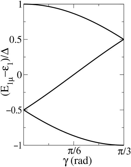
The interaction between dipole and quadrupole oscillations has been studied in the geometrical model. The coupling to the quadrupole degree of freedom splits the energy of the dipole mode, and within the linear coupling in the quadrupole amplitude[1] the energies of the three resulting dipole resonances as seen from the intrinsic frame are
| (1) |
where is the unperturbed dipole energy, is the restoring force parameter, and is the dipole–quadrupole coupling coefficient. A plot of these energies with respect to the unperturbed value is given in Fig. 1 as a function of the asymmetry parameter , for a fixed value of the quadrupole deformation parameter
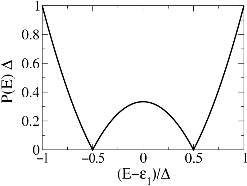
A detailed structure of the dipole absorption line can be obtained from a numerical diagonalization of the coupled dipole–quadrupole hamiltonian. A simple model in the strong coupling approximation for extracting the dipole strength distribution from the intrinsic values is provided by the procedure of averaging the three contributions over the different quadrupole and deformations, according to the ground state distribution. The relative strength of the dipole transition probability per unit of energy is in this way proportional to
| (2) |
where is the wave function of the ground state resulting from the quadrupole energy surface. The specific case of -unstable rotor occurs when the intrinsic energy surface is isotropic in the variable, while displaying a sharp minimum for deformation . Assuming the extreme situation of a very sharp minimum, we can in first approximation keep fixed the value of and only average over the variable. In this adiabatic picture one obtains the probability distribution shown in Fig. 2. The distribution is symmetric around , with three maxima, two at the edges (at energies ) and one in the center (at energy ), with
| (3) |
and with zeros occurring at energies . The resulting total splitting is therefore directly proportional to the quadrupole deformation , as in the case of a static quadrupole deformation. Note that although the probability at the edges is 3 times the one at the center, the total probability is anyway exactly equally divided into the three bumps. It may be worth noticing that, aside from the broadening of the three peaks, the predicted situation in the -unstable case is actually rather similar to the prediction associated with a static quadrupole deformed system with equal to 30 degrees. This similarity of the two situations is a feature that also appears for other observables and has been discussed elsewhere[16, 17].
III Coupling the dipole mode to an O(6) quadrupole deformed nucleus in IBM
To include the dipole degrees of freedom in the usual IBM, one negative parity dipole –boson () has to be included in addition to the positive parity quadrupole – () and – () bosons. For a boson system with quadrupole bosons plus dipole boson, the hamiltonian can be written as
| (4) |
where is the usual IBM hamiltonian for quadrupole degrees of freedom, is the dipole hamiltonian given by
| (5) |
and is the interaction between quadrupole and dipole degrees of freedom. The operator is the -boson number operator, which in this case is or , and is the unperturbed dipole energy. For the interaction a simple quadrupole-quadrupole form is assumed
| (6) |
where is the usual IBM quadrupole operator
| (7) |
and
| (8) |
The operators (where stands for , or bosons) are introduced so as to have operators with the appropriate properties under spatial rotations.
The simplest form for the dipole operator is
| (9) |
where is an overall normalization parameter, which will be assumed equal to unity in the applications.
A The coupling in the laboratory frame
First the laboratory IBM calculation is presented. The quadrupole hamiltonian for the O(6) limit can be written in the form
| (10) |
where stands for the quadratic Casimir operator of the indicated algebra as defined in Ref. [2]. Energies associated with this hamiltonian can be obtained analytically to be
| (11) |
where , and are the labels of the irreducible representations of the algebras O(6), O(5) and O(3) respectively. The coupling to the dipole oscillations and the calculation of transition probabilities is done numerically by using the computer codes GDR and GDRT, respectively [18].
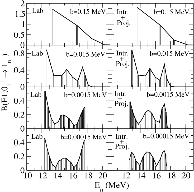
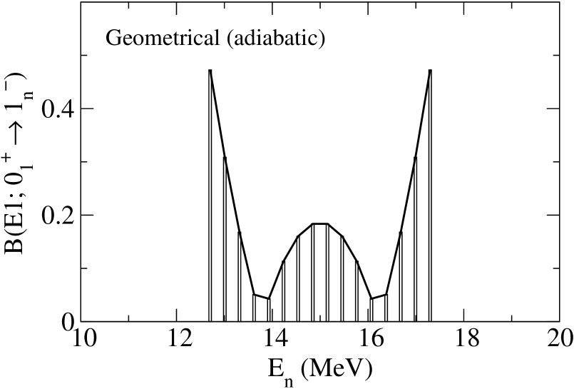
The states belonging to the representation are favoured in energy and the relative position of the states belonging to other representations is governed by the parameter . In the O(6) limit these representations are not connected by the quadrupole operator if is taken***With this choice the quadrupole operator is a generator of the O(6) algebra. in Eq. (7), and they therefore remain unmixed (and characterized by a good value of ) also with the inclusion of the dipole-quadrupole coupling. Consequently the dipole operator will only connect the ground state with states of the representation, which will therefore be the only ones contributing to the distribution. This implies that, as far as the dipole distribution is concerned, the calculation is completely insensitive to the value of the parameter . For the other parameters, in order to favour the comparison with preceding results obtained within the simple scheme based on the geometrical model, the parameter has been put equal to zero in order to minimize the splitting due to the angular momentum, a feature not accounted for by the unprojected intrinsic state. The results obtained for the energies of dipole states and the corresponding are shown in Fig. 3 (left panels) for different values of the parameter in front of the O(5) Casimir operator. At variance with the previous distribution displayed in Fig. 2 we have now a discrete distribution due to the finite number of bosons and consequently finite number of states. Note that the pure SU(3) limit with gives a dipole strength distribution with only two lines, since only two states can be obtained by coupling the dipole boson with the ground state rotational band. In the O(6) limit there are instead states connected to the ground state by the dipole operator, namely all those originated by the and states appearing in the band. We can however compare the envelope of this discrete distribution with the continuous distribution given by the geometrical model in its simplest adiabatic version. In order to facilitate comparisons an appropriate discretization of Fig. 2 for the case of N=15 bosons, an unperturbed dipole energy = 15 MeV, and a dipole-quadrupole coupling =0.2 MeV (same parameters as in Fig. 3) is presented in Fig. 4. In the limit of very small values of , namely in strong-coupling situations, the splitting due to the different values of within each O(6) representation is small compared to the coupling. As a consequence the patterns obtained in Figs. 3 and 4 are similar, since the mixing between the different states induced by the quadrupole-dipole interaction is large. At the other extreme, for values of large with respect to the dipole-quadrupole coupling the pattern observed in Fig. 3 becomes very asymmetric, tending to concentrate the transition strength onto the lowest state, washing out any resemblance with the one obtained in the geometrical model, Fig. 4, and giving rise to a situation close to the pure spherical case. In fact in this weak-coupling limit, because of the large splitting, only the lowest states have large overlaps with the initial s–d ground state.
For a better understanding of the situation we will study next the problem within the intrinsic frame in the IBM.
B The coupling in the intrinsic frame
Let us now study the problem of the coupling of quadrupole and dipole degrees of freedom in the intrinsic frame, within the IBM description. The basic idea of the intrinsic-frame formalism in this case is to consider that the pure quadrupole states of the ground “band” are globally described by a boson condensate of the form
| (12) |
where the basic boson is given by
| (13) |
and being obtained by minimizing the energy surface. In the case of SU(3) one has and , and the intrinsic state is fully representative of the ground-state rotational band. In the case of O(6), instead, one has , and the intrinsic state, which gives rise to a -independent energy surface, is associated with all states of the “band” corresponding to the representation. For the dipole part, the corresponding building blocks are , and . Thus, the three states provide with an intrinsic basis where the dipole-quadrupole states can be studied. In this basis, the pure and parts of the hamiltonian are diagonal and the only non-diagonal contributions come from the interaction term. The matrix elements needed in order are
| (14) |
where have already been calculated [19],
| (15) |
| (16) |
The matrix elements not specified are zero. The matrix elements of can be easily computed to be
| (17) | |||||
| (18) | |||||
| (19) |
All the remaining relevant matrix elements for our study are zero.
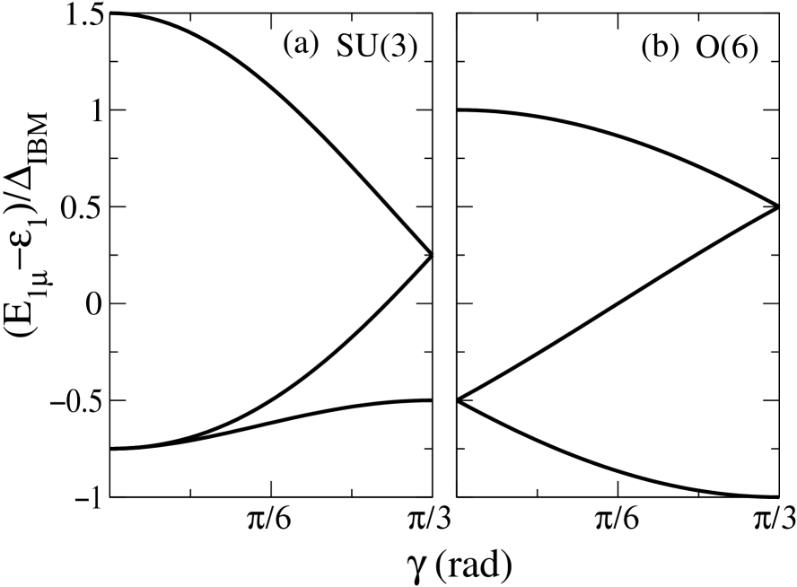
The parameter is the structure constant in the quadrupole operator . The SU(3) case (studied in Ref. [15]) is obtained for and the O(6) limit corresponds to . The dipole energies are obtained by diagonalising the interaction in the basis . They are analytically given by
| (20) | |||||
| (21) | |||||
| (22) |
which provide the dependence of the dipole energies on the IBM deformation parameters . With the choice , corresponding to the SU(3) limit, Eqs. (21) become equivalent to Eqs. (9b) in Ref. [15] with terms linear and quadratic in . The corresponding energies are shown in Fig. 5a. The O(6) limit corresponds instead to . In this case Eqs. (21) have only a linear term in , and the corresponding energies are shown in Fig. 5b. These latter energies are equal to those obtained in the preceding section for the geometrical model, once the correspondence is made between deformation parameters and coupling strengths in the two models, such that
| (23) |
As in the case of the geometrical model, a simple way of obtaining the dipole strength distribution from the IBM intrinsic state is to average the intrinsic energies over . In analogy to the intrinsic energies, the resulting distribution will show, mutatis mutandis, a pattern identical to the one shown in Fig. 2 for the geometrical model.
C Projection from the intrinsic frame to the laboratory
We have seen so far that the straightforward use of the intrinsic state in the IBM without any projection technique gives results similar to the ones obtained in the geometrical model. These results are consistent with those obtained in the laboratory frame only for boson hamiltonians that give rise to splittings in the elements of each O(6) multiplet which are much smaller than the splitting due to the dipole-quadrupole coupling. In all other more general cases, the effect of the breaking of degeneracy of each multiplet is essential, and proper treatment of the projection to the laboratory system from the intrinsic state is needed.
In this subsection it is therefore shown how to project the intrinsic state for the ground-state representation into the component. With this we would like to show that the calculations in the intrinsic frame, after projecting after on , reproduce the laboratory results. In the O(6) case the projector is known [20], and the important feature is that it produces exactly the laboratory states , belonging to the representation .
We have considered states of the form coupled to to total . The states are obtained by applying the projector (Bès functions [20]) to the intrinsic ground state as given in Eqs. (12,13). For each value of there is only one state (either or ) to be considered. Thus, for a given there will be dipole states.
In order to diagonalize the Hamiltonian in the subspace, we have included diagonal (trivial) and non–diagonal terms. For the latter ones we have used the results of the matrix elements of the interaction in the intrinsic frame (14-19) and made the appropriate integrations on and the Euler angles to go from the intrinsic to the laboratory frame. The resulting matrix to be diagonalized in the lab connects states of the same (diagonal terms) and states of with as known.
We have done full calculations up to for the case and found simple expressions for the non-diagonal matrix elements that allow calculations for any value of . These expressions are (we will use the notation for the states, with the selection rule = )
| (24) |
| (25) |
where . We have checked that these expressions coincide, in leading order in 1/N, with those associated with the corresponding “exact” states for and . With these matrix elements we have done a series of calculations and the resulting dipole distributions are compared in Fig. 3 (right panels) with the exact results in the laboratory frame for different values of . In Fig. 4 the corresponding distribution obtained from the unprojected intrinsic state (equal for all values of ) is plotted for comparison. In all the cases we have fixed the number of bosons to 15 and the intensity of the quadrupole ()-quadrupole () interaction to the value MeV. We have changed the intensity of the term by acting on the term in Eq. (10). In the following points we comment on the results given in Fig. 3.
-
i) MeV. This gives an excitation energy of the of 0.0012 MeV, almost degenerate case. The pattern of the in the exact calculation [18] (left lowest panel) is as mentioned before (three maxima, two at the edges with about 3 times the value of the maximum at the center). In our projected calculation (right lowest panel) we obtain similar pattern with three bumps but now the maxima at the edges are lower than in the full lab calculation and the maximum at the center is higher than the one in the exact calculation. In this way we obtain three maxima of roughly the same height. The two minima are more or less in the same places in both calculations. It is remarkable that the number of states in the projected calculation close to the edges is larger than in the full lab calculation and the number of states close to the center is smaller. In that way the summed values in each of the three bumps is the same in both calculations. The energy separation between edges is also about the same in both calculations.
-
ii) MeV. This gives an excitation energy of the of 0.012 MeV. Now the patterns are more similar in both calculations, the population of the lowest part being favoured in both cases. The results start to deviate appreciably from the unprojected ones.
-
iii) MeV. This gives an excitation energy of the of 0.120 MeV. Now the patterns of the laboratory and the projected intrinsic state are very close, with strong deviation from the pure results of the intrinsic state.
-
iv) MeV. This gives an excitation energy of the of 1.2 MeV. Now only the 3-4 lowest states are populated and energies and ’s are practically identical in both calculations.
From this comparison we conclude that our intrinsic calculation followed by projection on gives a good approximation to the laboratory results. It is worth noticing that in all cases the agreement is excellent except for the almost degenerate case, which is surprising since in that case the intrinsic state is expected to be a good approximation (see Fig. 3 lowest left panel and Fig. 4). This can be due either to the projection method or to the intrinsic trial wave function. In this case the projection method is known to be exact for the large limit, thus the problem must come from the trial wave function. As mentioned above, in the limit of very small values of (strong-coupling situations) the splitting of the different values of within each O(6) representation is small compared to the coupling. Consequently, the trial wave function proposed as with given by Eqs. (12,13) could be not completely appropriate in this case. The coupling to the additional dipole boson has in fact destroyed the full -unstability of the system (cf. Fig. 5), leading to an additional variation of the order of 1/ in the basic boson of the condensate. The situation is similar to that obtained, for example, in the coupling of an odd particle to a SU(3) boson core, where the additional particle slightly shiftes the position of the minimum of the energy surface in the - plane.
It should be noted that realistic cases of O(6) nuclei correspond to values of around MeV, far from degeneration in . We have checked this by making a set of calculations for a fixed and reasonable value of and changing the interaction . In those cases agreement between laboratory calculations and intrinsic plus projection is fine for any reasonable value of . Only for extremely large and unphysical values of some discrepancies between both calculations start to appear.
Once the energy spectra and the dipole transition strengths have been discussed we present in the next Section the cross sections for absorption of unpolarized radiation in the GDR region.
IV Photonuclear cross-section
Dipole strength distributions are traditionally measured in photoabsorption processes. Although photoabsorption cross-sections directly reflect the dipole strength, some of the features associated with this strength may disappear, be masked or modified by the effect of the finite widths. For this reason, once the distribution of the individual dipole states has been analyzed in the preceding section, we prefer in this section to compare results obtained within the IBM dipole model in the laboratory frame, unprojected and projected intrinsic frame directly for photoabsorption cross-sections.
The cross section for photoabsorption is in fact given by [21]
| (26) |
where are the widths of the dipole states at energy . The dipole widths are either taken as a constant or assumed to have a power law dependence on the energy,
| (27) |
where is the energy of the unperturbed dipole state and its width. Both and are used as adjustable parameters when one is fitting experimental data.
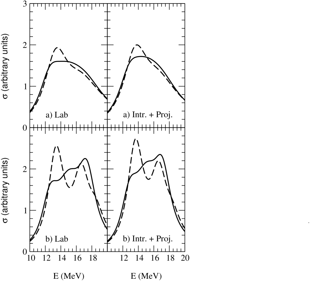
In Fig. 6 we present the cross-sections obtained for the two extreme (=0.00015 MeV and =0.15 MeV) dipole strength distributions corresponding to Fig. 3. Full lines give the results for the case =0.00015 MeV (almost -degenerate case) while dashed lines are for =0.15 MeV. In both cases MeV and the intensity of the quadrupole (sd)-quadrupole (p) interaction () is 0.2 MeV. Left panels give the laboratory results and right panels the intrinsic plus projection on results.
We have done two sets of calculations which select different widths for the dipole states. Upper panels correspond to the case in which the dipole widths are assumed to have a power law dependence on the energy. Since we are not working with an specific nucleus, we have taken = 0.026 (MeV) and =1.91. These values come from one global parametrization of experimental photoabsorption cross sections for [22]. That implies widths ranging from about 3.5 to 6.0 MeV for ranging from 13 to 17 MeV, respectively. Lower panels represent equivalent cases but taking the dipole widths as a constant equal to 2.5 MeV.
First of all we should realize that the actual shape of the photoabsorption cross-section is very much dependent on the widths assumed. The dashed lines (case with =0.15 MeV) in all panels still reflect contributions from the two lower states since they are separated by about 3 MeV. By contrast, all the states contribute to the almost degenerate case (full lines, =0.00015 MeV) since now the states differ by less than 0.5 MeV. Thus the image on the photoabsorption cross-section of the shape of the dipole strength distribution in Fig. 3 is diluted, even showing a plateau when we use the biggest widths (upper panels).
In all the cases, independently of the election of and the dipole widths assumed (either constant or energy dependent), a good agreement between the laboratory and -projected intrinsic frame calculations is observed when comparing left and right panels, although as in Fig. 3 as the absolute value of the ratio b/ decreases its quality becomes a bit worse. It is worth noticing that the calculations for the case of unprojected geometrical adiabatic situation given in Fig. 4 are indistinguishable from those plotted with full line on the right-hand-side panels (=0.00015 MeV) as expected.
V Summary and conclusions
We have studied the problem of the coupling of the quadrupole and dipole oscillations in -unstable nuclei in the framework of the IBM. We have obtained and explained the results in the laboratory by studying the problem in the intrinsic frame taking at higher order the non-degeneracy in .
In the -degenerate limit the dipole mode total splitting (2) turns out to be proportional to the dipole-quadrupole coupling strength, the number of sd bosons considered, N, and the quadrupole deformation. Furthermore, the dipole mode splits in N+1 lines and its distribution is symmetric around the unperturbed dipole energy. This symmetry is destroyed as soon as we allow non-degeneracy in , giving rise to a very asymmetric distribution. In the weak coupling limit the transition strength is concentrated onto the lowest states. Since this limit seems to correspond to the actual situation in typical O(6) nuclei, 196Pt or 134Ba for instance, the explicit treatment of the non-degeneracy in is crucial. In this case the results from the geometrical model in the adiabatic limit are quite different from the dipole boson model ones. In this sense, the O(6) limit is different to the SU(3) case in which the rotational excitation energy is low and can be ignored in first approximation and, consequently, the geometrical model in the adiabatic limit gives an appropriate description.
Calculations of photoabsorption cross-sections using the intrinsic state in the IBM followed by projection on give a good approximation to the laboratory results. No experimental data on O(6) nuclei are available and they could be valuable to elucidate whether the dipole strength distribution in actual O(6) nuclei is in agreement with the -projected dipole boson model results presented here.
Acknowledgments
This work was supported in part by a Spanish–Italian CICYT-INFN agreement and by the Spanish DGICYT under project number PB98-1111. Part of this work was done while E.G.L. was at Sevilla University as a Marie Curie Fellow with contract ERBFMBICT-983090. We acknowledge useful discussions with F. Iachello and A. Leviatan. We thank P. Van Isacker for providing us with the IBM codes GDR and GDRT.
REFERENCES
- [1] A. Bohr and B. Mottelson, Nuclear Structure, vol II, Benjamin, Reading, Mass. 1975
- [2] F. Iachello and A. Arima, The interacting boson model, Cambridge University Press, Cambridge, England, 1987
- [3] L. Wilets and M. Jean, Phys. Rev. 102 (1956) 788.
- [4] A. Arima and F. Iachello, Ann. Phys. (N.Y.) 99 (1976) 253.
- [5] A. Arima and F. Iachello, Ann. Phys. (N.Y.) 111 (1978) 201.
- [6] A. Arima and F. Iachello, Ann. Phys. (N.Y.) 123 (1979) 468.
- [7] J. N. Ginocchio and M. W. Kirson, Nucl. Phys. A 350 (1980) 31.
- [8] A. E. L. Dieperink, O. Scholten and F. Iachello, Phys. Rev. Lett. 44 (1980) 1747.
- [9] A. Bohr and B. Mottelson, Phys. Scripta 22 (1980) 468.
- [10] M. Danos and W. Greiner, Phys. Lett. 8 (1964) 113.
- [11] M. Danos and W. Greiner, Phys. Rev. B 134 (1964) 284.
- [12] I. Morrison and J. Weise, J. of Phys. G 8 (1982) 687.
- [13] F. G. Scholtz and F. J. W. Hahne, Phys. Lett. B 123 (1983) 147.
- [14] G. Maino, A. Ventura, L. Zuffi and F. Iachello, Phys. Rev. C 30 (1984) 2101.
- [15] F. G. Scholtz and F. J. W. Hahne, Nucl. Phys. A 471 (1987) 545.
- [16] M. Sugita, A. Gelberg and T. Otsuka, Nucl. Phys. A 567 (1994) 33.
- [17] N. Yoshida, A. Gelberg, T. Otsuka, I. Wiendenhöver, H. Sagawa and P. von Brentano, Nucl. Phys. A 619 (1997) 65.
- [18] P. Van Isacker, Fortran Computer Codes GDR and GDRT, unpublished.
- [19] C. E. Alonso, J. M. Arias, F. Iachello and A. Vitturi, Nucl. Phys. A 539 (1992) 59.
- [20] D. Bès, Nucl. Phys. 10 (1959) 373.
- [21] V. Redwani, G. Gneuss and H. Arenhövel, Nucl. Phys. A 180 (1972) 254.
-
[22]
Reference Input Parameter Library for Theoretical Calculation of
Nuclear Reactions (RIPL Handbook), Chapter 6: Gamma-Ray Strength
Functions.
http://www-nds.iaea.or.at/ripl/