Theoretical description of deformed proton emitters:
nonadiabatic coupled-channel method

Abstract

The newly developed nonadiabatic method based on the coupled-channel Schrödinger equation with Gamow states is used to study the phenomenon of proton radioactivity. The new method, adopting the weak coupling regime of the particle-plus-rotor model, allows for the inclusion of excitations in the daughter nucleus. This can lead to rather different predictions for lifetimes and branching ratios as compared to the standard adiabatic approximation corresponding to the strong coupling scheme. Calculations are performed for several experimentally seen, non-spherical nuclei beyond the proton dripline. By comparing theory and experiment, we are able to characterize the angular momentum content of the observed narrow resonance.

]

I Introduction

Nuclei beyond the proton dripline are unstable against proton emission. Although formally unbound, some of these systems have rather long lifetimes, ranging from microseconds to seconds, due to the confining effect of the Coulomb barrier [1, 2].

The past few years have seen an explosion of exciting discoveries in this field including new ground-state and isomeric proton emitters [3, 4, 5, 6] and the first evidence for fine structure in proton decay [7]. The focus of recent investigations has been on well-deformed nuclei which exhibit collective motion. These are of particular interest due to the interplay between proton emission and angular momentum.

The theoretical description of long-lived proton emitters requires a detailed understanding of narrow resonances. Although proton radioactivity is a complicated $A$-body phenomenon, much insight may be gained by considering the simplified problem of a single proton penetrating the Coulomb barrier of the core consisting of the remaining $A$–1 nucleons. It has been found that this simple one-body picture works surprisingly well. In many cases one has been able to determine the angular momentum content of the resonance and the associated spectroscopic factor [2].

For spherical systems, there are many methods on the market which give similarly precise descriptions and, in many cases, one has been able to determine the angular momentum content of the resonance and the associated spectroscopic factor [2, 8].

The array of theoretical tools available for deformed emitters is not as well developed. The existing ones fall into three general categories. The first family of calculations [3, 7, 9] is based on the reaction-theoretical framework of Kadmenskiĭ and collaborators [10]. The second suite uses the theory of Gamow (resonance) states [5, 11, 12, 13]. Finally, an approach, based on the time-dependent Schrödinger equation, has been introduced in Ref. [14].

In all of these previous attempts, the strong coupling approximation of the particle-plus-rotor model has been used. The core is taken to be a perfect rotor with infinite moment of inertia. This has the effect of (i) collapsing the rotational spectrum of the daughter nucleus to the ground state and (ii) neglecting the Coriolis coupling. Recently we have introduced a technique based on the weak coupling scheme which is free from these deficiencies [15]. Within this method, partial proton widths from different states of the parent nucleus to various final states in the daughter system can be calculated in a straightforward and consistent manner.

We will begin in Sec. II by laying the theoretical framework for this work. Section III discusses the numerical methods adopted in our work. Section IV presents application of the method to the structure of deformed proton emitters. A critical analysis of the adiabatic and nonadiabatic methods is contained in Sec. V. Finally, conclusions are given in Sec. VI.

II Theoretical Basis

From a theoretical point of view, proton radioactivity is an excellent example of three-dimensional, quantum-mechanical tunneling. As such, the understanding of proton emission is really a test of our knowledge of very narrow resonances. Since the lifetimes which can be seen experimentally range from microseconds to seconds, the corresponding widths are extremely small; they vary between $10^{-16}$ MeV and $10^{-22}$ MeV. Theoretical description of such small widths requires high numerical accuracy. In the following, the coupled-channel Schrödinger equation method with Gamow states is outlined, and the proton-plus-core Hamiltonian is defined.

A Coupled-channel Equations

The parent nucleus is described by the core-plus-proton Hamiltonian,

$$H=H_{d}+H_{p}+V,$$ (1)

where $H_{d}$ is the Hamiltonian of the daughter nucleus, $H_{p}$ is that of the proton, and $V$ is the proton-daughter interaction. In the weak coupling scheme, the wave function of the parent nucleus is written as

$$\Psi_{JM}=r^{-1}\sum_{J_{d}l_{p}j_{p}}u_{J_{d}l_{p}j_{p}}^{J}(r)\left({\cal Y}_{l_{p}j_{p}}\otimes\Phi_{J_{d}}\right)_{JM}.$$ (2)

This wave function is labeled by parity, total angular momentum $J$, and its projection $M$. In Eq. (2), $u_{\alpha}^{J}(r)$ [where $\alpha\equiv(J_{d}l_{p}j_{p})$ completely labels the channel quantum numbers] is the cluster radial wave function representing the relative radial motion of the proton and the core, and ${\cal Y}_{l_{p}j_{p}m_{p}}$ is the orbital-spin wave function of the proton. The daughter wave function, $\Phi_{J_{d}M_{d}}$, satisfies

$$H_{d}\Phi_{J_{d}M_{d}}=E_{J_{d}}\Phi_{J_{d}M_{d}}.$$ (3)

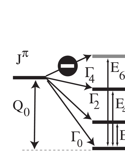
In the present formalism, the daughter’s spectrum does not have to be known explicitly. Where possible, the energies $E_{J_{d}}$ are taken from experiment; otherwise, the spectrum is modeled theoretically. Figure 1 shows a schematic diagram illustrating the energetics of proton emission from a $J^{\pi}$ state of an odd-$Z$ parent nucleus to the ground-state rotational band of the deformed daughter nucleus.

FIG. 1.: Schematic diagram illustrating the energetics of proton decay. A $J^{\pi}$ state of an odd-$Z$ parent nucleus (left) decays to those members of the ground-state rotational band of the even-even deformed daughter nucleus (right) which are in the $Q$ window. The band members have excitation energies $E_{J_{d}}$ relative to the ground state, and $Q_{0}$ is the $Q_{p}$ value for the decay to the ground state. As shown here, usually only a few channels are energetically open. The corresponding partial widths are indicated by $\Gamma_{J_{d}}$.

As usual, the coupled-channel equations are obtained by inserting Eq. (2) into the Schrödinger equation and integrating over all coordinates, save the radial variable $r$ [9, 16]:

$$\left[-\frac{\hbar^{2}}{2\mu}\frac{d^{2}}{dr^{2}}\right. + \left.\frac{\hbar^{2}l_{p}(l_{p}+1)}{2\mu r^{2}}+V_{\alpha\alpha}(r)-Q_{J_{d}}\right]u_{\alpha}^{J}(r)$$ (4)

$$+ \sum_{\alpha^{\prime}\neq\alpha}V_{\alpha,\alpha^{\prime}}^{J}(r)\;u_{\alpha^{\prime}}^{J}(r)=0.$$ (5)

In Eq. (4), $V_{\alpha\alpha}$ is the diagonal part of the proton-core potential, $Q_{J_{d}}$ is the energy of the emitted proton leaving the daughter nucleus in the state $J_{d}$, and $V^{J}_{\alpha\alpha^{\prime}}$ are the off-diagonal coupling terms. The $Q_{J_{d}}$ values follow from the spectrum of the daughter nucleus, $Q_{J_{d}}=Q_{0}-E_{J_{d}}$, where $Q_{0}$ is the $Q_{p}$ value for the decay to the $0^{+}$ ground state (see Fig. 1).

To illuminate the dynamics of the system, one can expand the proton-daughter potential in multipoles [16],

$$V=\sum_{\lambda}v_{\lambda}(r)\,({\hat{\cal M}}_{\lambda}\otimes Y_{\lambda})_{00}.$$ (6)

The matrix elements $V_{\alpha,\alpha^{\prime}}^{J}(r)$ can then be written in the simple, yet generic, form

$$V_{\alpha,\alpha^{\prime}}^{J}(r)=\sum_{\lambda}v_{\lambda}(r)\;\langle J_{d}||{\hat{\cal M}}_{\lambda}||J^{\prime}_{d}\rangle\;{\cal A}(l_{p}j_{p}J_{d},\,l^{\prime}_{p}j^{\prime}_{p}J^{\prime}_{d},\,\lambda J).$$ (7)

The factor $\cal A$ is purely geometric and comes from the proper coupling of angular momentum vectors. The reduced matrix elements of ${\hat{\cal M}}_{\lambda}$ contain all of the dynamics of the core. Since we consider only rotational nuclei in this paper, they are given by a simple expression [16]

$$\langle J_{d}||{\hat{\cal M}}_{\lambda}||J^{\prime}_{d}\rangle=\sqrt{2J^{\prime}_{d}+1}\;\langle J^{\prime}_{d}\lambda\;K0|J_{d}K\rangle.$$ (8)

To consider other excitation modes in the daughter system, one needs only change these reduced matrix elements.

To be a resonant state, the cluster radial wave function must vanish at the origin and behave as an outgoing Coulomb wave, $O_{l}=G_{l}+iF_{l}$, beyond the range of the nuclear interaction and the off-diagonal Coulomb interaction,

$$u^{J}_{J_{d}l_{p}j_{p}}(r) \stackrel{{\scriptstyle{\rm large}\;r}}{{\longrightarrow}} O_{l_{p}}(\eta_{J_{d}},r{k_{J_{d}}})$$ (9)

$$= G_{l_{p}}(\eta_{J_{d}},r{k_{J_{d}}})+iF_{l_{p}}(\eta_{J_{d}},r{k_{J_{d}}}),$$ (10)

where ${k_{J_{d}}}^{2}=2\mu Q_{J_{d}}/\hbar^{2}$ and $\eta_{J_{d}}{k_{J_{d}}}=\mu Ze^{2}/\hbar^{2}$. These two conditions are only satisfied for a discrete set of complex wave numbers $k$. The generalized eigenvalues of Eq. (4) correspond to the poles of the scattering matrix [17, 18]. The corresponding solutions are either bound or antibound states, ${\cal E}=E_{b}<0$, with negative real energies and imaginary wave numbers $k=i\gamma$ ($\gamma>0$ for bound and $\gamma<0$ for antibound states ), or resonance states, ${\cal E}=Q-i{\Gamma\over 2}$, with a nonzero imaginary part $\Gamma\neq 0$, and $k=\kappa-i\gamma$.

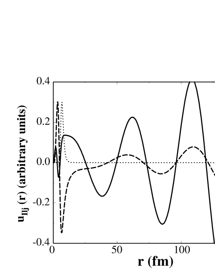
The asymptotic behavior of these solutions is determined by $k$; at a very large distance the outgoing solution is proportional to $e^{ikr}$. For resonance states, $e^{ikr}=e^{i\kappa r}e^{\gamma r}$, i.e., the wave function diverges exponentially. As discussed in Refs. [17, 18], this seemingly unphysical feature of Gamow wave functions has a natural explanation in the fact that Gamow states do not represent time-dependent wave packets but static sources. To illustrate the asymptotic behavior of Gamow wave functions, Fig. 2 shows three-channel wave functions corresponding to a broad neutron resonance.

FIG. 2.: Asymptotic behavior of three-channel wave functions corresponding to the $J^{\pi}$=$3/2^{-}$ neutron resonance in ¹⁴¹Ho at energy ${\cal E}=(0.378-i0.0732$) MeV calculated at $\beta_{2}$=0.20. The solid line denotes the $p_{3/2}\otimes 0^{+}$ channel. Notice the increasing envelope for increasing $r$. The dashed line labels the $f_{5/2}\otimes 2^{+}$ channel function. The dotted line corresponds to the closed channel $l_{19/2}\otimes 8^{+}$. The wave function decays exponentially since $Q<0$. The magnitude has been scaled so all three wave functions could be shown.

Due to the divergent behavior at large $r$, one must define a new normalization scheme for the Gamow states. Berggren proposed a new completeness relation, which includes Gamow states [19], by generalizing the scalar product. He introduced a bilinear basis set and a regularization procedure (${{\cal R}eg}$). With this generalization, the norm is

$$\sum_{\alpha}{{\cal R}eg}\int_{0}^{\infty}[u^{J}_{\alpha}(r)]^{2}\,dr=1.$$ (11)

A convenient method for regularization is to rotate $r$ into the first quadrant of the complex $r$-plane beyond a certain distance $r_{\rm max}$. This is often referred to as the exterior complex scaling method. (For other regularization techniques, see Ref. [18].)

Once we know the resonance energy and radial wave functions, there are several methods to calculate the width of the state. The most straightforward method is to take twice the negative of the imaginary part of the resonance energy. However, for the narrow resonances associated with proton emitters, the numerical accuracy needed to calculate ${\cal I}{\rm m}[{\cal E}]$ is difficult to achieve. Therefore, approximate methods are often used.

One possibility is to calculate the partial width for each channel from the current expression [17],

$$\Gamma_{\alpha}(r)=i\frac{\hbar^{2}}{2\mu}\frac{u_{\alpha}^{\prime*}(r)u_{\alpha}(r)-u^{\prime}_{\alpha}(r)u_{\alpha}^{*}(r)}{\sum_{\alpha^{\prime}}\int_{0}^{r}|u_{\alpha^{\prime}}(r^{\prime})|^{2}{\rm d}r^{\prime}},$$ (12)

where the sum of the partial widths,

$$\Gamma(r)=\sum_{\alpha}\Gamma_{\alpha}(r),$$ (13)

gives the total decay width (see Fig. 1). Although values of $\Gamma_{\alpha}(r)$ depend on $r$ in the region $r$$<$$r_{\rm as}$ where the coupling potential terms are not negligible, $\Gamma(r)$ is strictly independent of $r$ by construction ($\Gamma(r)=-2{\cal I}{\rm m}[{\cal E}]=\Gamma$) which reflects the flux conservation (continuity equation). Beyond the asymptotic radius, $r_{\rm as}$, the partial widths, $\Gamma_{\alpha}(r)$ have a negligible dependence on radius. We take $r_{\rm as}\approx 40$fm. Numerically, $\Gamma(r)$ varies little with distance and differs by less than $0.1\%$ from the $\Gamma$ obtained from the imaginary part of the eigenvalue.

The Gamow boundary condition given by Eq. (9) is usually written in the form

$$\frac{u^{\prime}_{\alpha}(r_{\rm as})}{u_{\alpha}(r_{\rm as})}={k_{J_{d}}}\frac{O^{\prime}_{l_{p}}(\eta_{J_{d}},r_{\rm as}{k_{J_{d}}})}{O_{l_{p}}(\eta_{J_{d}},r_{\rm as}{k_{J_{d}}})},$$ (14)

where $r_{\rm as}$ is the channel radius. (The off-diagonal couplings are negligible beyond it.) Using Eq. (14), the partial decay widths can be written at the point $r_{\rm as}$ as

$$\Gamma_{\alpha}(r_{\rm as}) = i\frac{\hbar^{2}}{2\mu}\frac{|u_{\alpha}(r_{\rm as})|^{2}}{|O_{l_{p}}(\eta_{J_{d}},{k_{J_{d}}}r_{\rm as})|^{2}\sum_{\alpha^{\prime}}\int_{0}^{r_{\rm as}}|u_{\alpha^{\prime}}(r^{\prime})|^{2}{\rm d}r^{\prime}}$$ (15)

$$\times \left[k_{J_{d}}^{*}O^{\prime*}_{l_{p}}(\eta_{J_{d}},r_{\rm as}{k_{J_{d}}})O_{l_{p}}(\eta_{J_{d}},r_{\rm as}{k_{J_{d}}})\right.$$ (16)

$$- \left.{k_{J_{d}}}O^{\prime}_{l_{p}}(\eta_{J_{d}},r_{\rm as}{k_{J_{d}}})O^{*}_{l_{p}}(\eta_{J_{d}},r_{\rm as}{k_{J_{d}}})\right].$$ (17)

If we neglect the very small imaginary part of ${k_{J_{d}}}$, the square bracket in Eq. (15) is equal to $-2i$. Furthermore, if we assume that for a very narrow resonance the imaginary part of $u_{\alpha}$ is very small (hence the generalized normalization condition (11) is roughly equivalent to the “normal” normalization $\sum_{\alpha^{\prime}}\int_{0}^{r_{\rm as}}|u_{\alpha^{\prime}}(r^{\prime})|^{2}dr^{\prime}\approx 1$), then we end up with the approximate expression for the partial decay width:

$$\Gamma_{\alpha}(r_{\rm as})\approx\frac{\hbar^{2}\kappa_{J_{d}}}{\mu}\frac{|u_{\alpha}(r_{\rm as})|^{2}}{|O_{l_{p}}(\eta_{J_{d}},{k_{J_{d}}}r_{\rm as})|^{2}}.$$ (18)

It is to be noted that Eq. (15) and its approximate form (18) are valid only at the point $r_{\rm as}$. The expression (18) was used in papers [12, 13, 20, 21]. We emphasize that if the coupled equations are solved with the Gamow boundary condition, then the total width can be calculated at any intermediate point using Eqs. (12) and (13). The expression (18) is very similar to that of the R-matrix theory (see below), but it relies on different approximations and boundary conditions than the R-matrix formalism.

In the R-matrix theory, we also have a set of radial functions, $g_{\alpha}$. These functions are regular at the origin and satisfy the coupled equations but with the following boundary conditions:

$$r_{\rm as}\frac{g^{\prime}_{\alpha}(r_{\rm as})}{g_{\alpha}(r_{\rm as})}=B_{\alpha},$$ (19)

where $B_{\alpha}$ are arbitrary real numbers. Due to the real boundary condition, the R-matrix eigenvalues are real numbers. In the R-matrix theory, the wave function is normalized inside the sphere of radius $r_{\rm as}$, i.e., $\sum_{\alpha}\int_{0}^{r_{\rm as}}|g_{\alpha}(r)|^{2}dr=1$. Thomas has shown [22] that in a one-level approximation with appropriately chosen $B_{\alpha}$, in which the level shift is ignored, the position of the Gamow resonance corresponds to the R-matrix eigenvalue, and the width of the state can be calculated in the form given by Eq. (18) in which $u_{\alpha}(r)$ is replaced with $g_{\alpha}(r)$. This R-matrix approximation works fairly well [23, 24] for very narrow Gamow resonances corresponding to the known proton emitters. For large values of the channel radius $r_{\rm as}$, expression (18) is generally within 2% of the values calculated explicitly from Eq. (4) or obtained via the current expression (12). a detailed comparison of the R-matrix theory and the Gamow formalism for proton emitters will be given in Ref. [25].

The nonadiabatic approach allows for a straightforward calculation of branching ratios. The partial width corresponding to the decay to a core state $J_{d}$ is given by

$$\Gamma_{J_{d}}=\sum_{\{lj\}}\Gamma_{{J_{d}}lj},$$ (20)

where $\Gamma_{{J_{d}}lj}=\Gamma_{\alpha}$ is given by Eq. (12). Once the total width is known, the half-life for proton emission is

$$T_{{\frac{1}{2}}}=\frac{\hbar\ln 2}{\Gamma}.$$ (21)

The use of the weak coupling scheme represented by Eq. (2) has several advantages. First, excitations of the core are included in a straightforward manner. This enables us to study the proton decay from the rotational bands of the parent nucleus to the ground-state rotational band of the daughter nucleus. Furthermore, since the formalism is based on the laboratory-system description [Hamiltonian (1) is rotationally invariant and the wave function $\Psi_{JM}$ conserves angular momentum], the Coriolis coupling is automatically included.

B Strong Coupling Limit

A great simplification to Eq. (4) occurs if one considers all of the rotational states in the daughter’s ground-state band to be degenerate (i.e., $Q_{J_{d}}\equiv Q_{p}$ for all $J_{d}$). This is the limit of strong coupling where the moment of inertia of the daughter is taken to infinity. It is also the adiabatic approximation of Refs. [16, 26].

In this limit, the coupled-channel equations, (4), reduce to those for the intrinsic (i.e., deformed) Nilsson orbital [9]

$$\Psi_{\Omega}=\sum_{j_{p}l_{p}}\frac{u_{\Omega\Omega j_{p}l_{p}}(r)}{r}{\cal Y}_{l_{p}j_{p}\Omega}$$ (22)

where

$$u_{JK\,j_{p}l_{p}}=\sqrt{2}\ (-1)^{K+J}\sum_{J_{d}}\langle J_{d}0j_{p}K|JK\rangle u^{J}_{J_{d}l_{p}j_{p}}.$$ (23)

In Eq. (22) $\Omega$=$K$=$J$ is the angular momentum projection on the symmetry axis. As seen from Eq. (23), the strongly coupled intrinsic state contains contributions from all the cluster wave functions corresponding to different core states. Since, as discussed by Tamura[16], there is no dynamic coupling between the angular momentum of the proton and that of the daughter nucleus (the daughter nucleus is perfectly inert during the proton emission), there exist infinitely many solutions obtained by combining $\mathchoice{{\hbox{\boldmath$\displaystyle j$}}}{{\hbox{\boldmath$\textstyle j$}}}{{\hbox{\boldmath$\scriptstyle j$}}}{{\hbox{\boldmath$\scriptscriptstyle j$}}}_{p}$ and $\mathchoice{{\hbox{\boldmath$\displaystyle J$}}}{{\hbox{\boldmath$\textstyle J$}}}{{\hbox{\boldmath$\scriptstyle J$}}}{{\hbox{\boldmath$\scriptscriptstyle J$}}}_{d}$. Since the core states are degenerate, all the solutions with $J\geq\Omega$ are degenerate as well.

C Model Parameters

FIG. 3.: Comparison of deformed single-proton levels for $Z=63,N=68$ predicted in three WS parameterizations. The left panel shows the Nilsson diagram calculated with the Becchetti-Greenlees set which yields poor ordering of the single-particle levels but good radial properties. The right panel is obtained with the “universal” set which yields good ordering of Nilsson levels but poor radial properties of wave functions. The center panel was obtained with the Chepurnov parameter set used in this work. This latter parameterization gives a very reasonable compromise between the radial and spectroscopic properties.

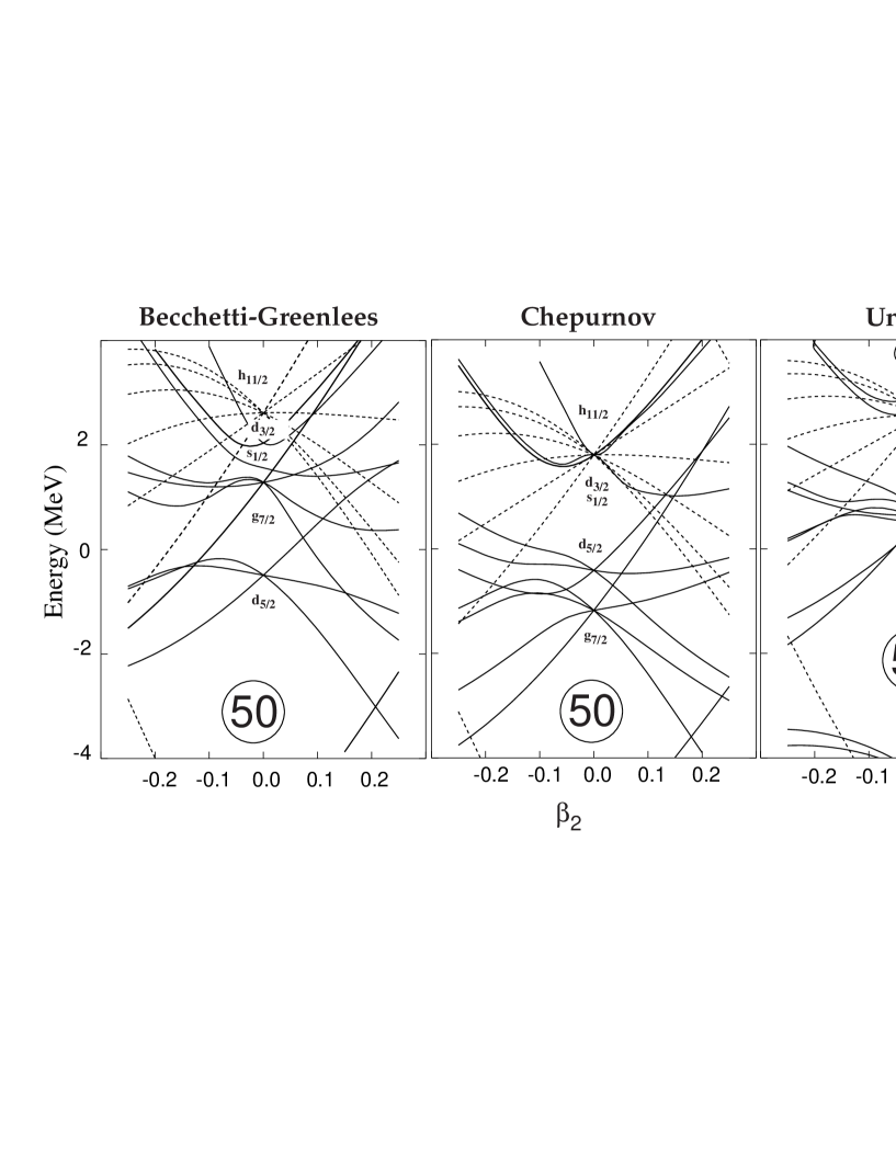
In this work, we assume that the average single-particle potential is approximated by the sum of a Woods-Saxon (WS) potential, a spin-orbit term, and a Coulomb potential. The axially deformed WS potential is defined according to Ref. [27]. We employ the Chepurnov parameterization [28]; it is in good agreement with the proton single-particle energy levels given in the systematic study [29]. Åberg et al. [8] discussed the effect of the optical model parameters on spherical proton emitters. They concluded that the uncertainties in the parameters affect the half-lives by, at most, a factor of 3. For spherical proton emitters, they concluded that the Becchetti-Greenlees WS potential [30], commonly used in spherical calculations for proton emitters, was better than the universal parameter set [31] (excellent for the description of structure properties of deformed rare-earth nuclei [29] but having too large a radius to give a quantitative description of the tunneling rate). Since, for the description of spherical proton emitters, the nodal behavior of radial wave functions plays a minor role [8], the actual order of spherical shells does not really matter.

However, in the case of deformed proton emitters the situation is different. While the radial properties of the optical model potential are still important, the proper ordering of spherical shells becomes crucial since it affects the fragmentation of orbital angular momentum caused by deformation. In this context, as illustrated in Fig. 3, the Becchetti-Greenlees parameter set performs rather poorly, while the Chepurnov parameterization offers a compromise between good radial properties and proper level ordering.

Since within any mean-field theory the resonance energy cannot be predicted with sufficient accuracy, following Refs. [5, 8], the depth of the WS potential is adjusted to give the experimental $Q_{0}$ value. The deformed part of the spin-orbit interaction is neglected; we do not expect this to have a noticeable effect on the results [32]. The off-diagonal coupling in (4) appears thanks to the non-spherical parts of the WS and Coulomb potentials.

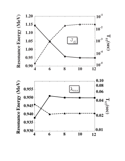
Great care was taken to ensure that enough channels were considered in solving Eq. (4) for proper convergence in the eigenvalues. As seen in the lower panel of Fig. 4, expanding the WS in spherical multipoles to order 8 is sufficient for convergence. However, to be on the safe side, a value of $\lambda_{\rm max}=12$ in Eq. (6) was used in all calculations. The number of partial waves that were needed in the decomposition of the proton radial wave function varies from system to system depending mainly on the angular momentum of the proton state. In general, all partial waves with $l$$<$10–13 are needed. Since, in the nonadiabatic approach, the maximum proton angular momentum and the maximum daughter spin considered are closely related, the above condition corresponds to $(J_{d})_{\rm max}=10$ which was used for all calculations (see upper panel of Fig. 4). Since the high-spin channels are energetically forbidden, their exact placement is of minor importance. Only the energy of the $2^{+}$ level and, occasionally, the $4^{+}$ level have a profound effect on the resonance energy and other observable quantities. (For more discussion concerning this point, see Sec. V.)

FIG. 4.: Dependence of the resonance eigenstate on various expansion parameters. Calculations were done for the $[411]{\frac{3}{2}}$ level in ¹³¹Eu at a deformation of $\beta_{2}=0.37$. The upper panel shows the resonance energy (solid line with squares and left scale) and the lifetime (dashed line with triangles and right scale) as a function of the number of included states in the ground-state band of the daughter nucleus. The lower panel shows the same except as a function of the number of spherical multipoles used in expanding the deformed single-particle potential.

It is important in this work that we have a good representation of the ground-state rotational band in the daughter nucleus. In a few of the systems studied in this work, such spectra exists for $J_{d}\leq 10$, which is enough for adequate convergence. However, for the most highly deformed systems, the spectroscopic information does not exist. For these nuclei, we parameterize the ground-state rotational band as $E_{J_{d}}$= $\kappa J_{d}(J_{d}+1)$, where $\kappa$ is adjusted to the $E_{2^{+}}$ energy. In ¹³¹Eu, where fine structure has been seen, the $E_{2^{+}}$ energy is known. In other cases, systematic trends must be used. In actual calculations, we have used the $N_{p}N_{n}$ scheme [33] to estimate $E_{2^{+}}$.

III Numerical Implementation

For realistic potentials, the radial Schrödinger equation cannot be solved analytically but must be integrated numerically. For spherical potentials, one deals with a single radial equation instead of the full set (4). In Ref. [34] the code GAMOW was introduced, which uses the Fox-Goodwin method for solving the radial equation. A more powerful method, the piecewise perturbation, is used for the same purpose in Ref. [35]. The main features are similar in the two codes. The total $r$ domain of coupled-channel equations (4) is separated into two parts. The first segment lies along the real axis, $I_{1}=[0,r_{\rm max}]$. The other interval extends along the complex ray, $I_{2}=[r_{\rm max},r_{\rm as}]$, where $r_{\rm as}$ is complex and far enough away that at $r_{\rm as}$ the asymptotic series of the outgoing Coulomb wave, $O_{l}(\eta_{J_{d}},r_{\rm as}{k_{J_{d}}})$, is a good approximation. For a resonant state, the second integration region must be complex for our regularization scheme given by Eq. (11). The rotation angle of $r$ in $I_{2}$ should satisfy the condition

$$\pi-\arg({k_{J_{d}}})>\arg(r_{\rm as})>-\arg({k_{J_{d}}})$$ (24)

so that the solution converges along the complex ray.

For axially deformed $V$, the set of coupled-channel equations (4) must be solved numerically. The piecewise perturbation method [36] has been generalized for the coupled-channels case [37]. A large value of $r_{\rm as}$ is used, which is far enough away that the off-diagonal terms of the coupling matrix vanish and the asymptotic series for the Coulomb functions are accurate. At this point the coupled-channels equations decouple. For an initial ${k_{J_{d}}}$ value, one has to calculate the components of a “left” solution, $u_{\alpha}^{L}$, which vanish at the origin. These are integrated outwards to a matching radius, $r_{\rm m}$, in region $I_{1}$. The components of the “right” solutions, $u_{\alpha}^{R}$, are integrated inwards from $r_{\rm as}$ along the complex ray $I_{2}$. At $r_{\rm max}$, the integration path turns along the real axis to the matching radius, $r_{\rm m}$. All components of the “left” and “right” solutions are linear combinations of linearly independent solutions of Eq. (4) in the corresponding $r$ regions. The two solutions and their derivatives with respect to $r$ should match at the matching radius and form a set of functions which are continuous in $r$. This condition gives a homogeneous set of linear equations for the unknown expansion coefficients of $u_{\alpha}^{L}$ and $u_{\alpha}^{R}$. Non-trivial solutions exist only for the generalized ${k_{J_{d}}}$ eigenvalues where the determinant of the set of linear equations is equal to zero. For the initial value of ${k_{J_{d}}}$, the determinant is not zero; however, it is possible to find the zero of the determinant by iteration, e.g., using the Newton–Raphson method. For the known proton emitters, the width of the resonance is so small that extremely high numerical accuracy is needed to calculate the generalized complex energy eigenvalue ${\cal E}$. We have found that extended precision arithmetic must be employed to calculate the imaginary part of ${\cal E}$ accurately. The width calculated directly in this manner matches well with the current expression (12).

IV Applications of the Method

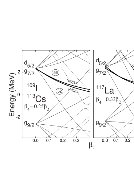
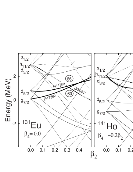
This section contains applications of the formalism to measured deformed proton emitters. For an easy orientation, Figs. 5 and 6 show the proton Nilsson diagrams characteristic of $Z$$\approx$55 and $Z$$\approx$67 nuclei, respectively. In our theoretical analysis, all Nilsson levels close to the Fermi level were investigated. The potential depth was always adjusted at each deformation so as to reproduce the experimental $Q_{p}$ value. Table I lists the $Q_{p}$ values, the energy of the $2^{+}$ states, and deformation parameters for all the nuclei investigated in this paper.

FIG. 5.: Single-proton levels representative of odd-$Z$ rare-earth nuclei with $Z$$\approx$55 plotted as functions of the quadrupole deformation $\beta_{2}$. The hexadecapole deformation $\beta_{4}$ was assumed to be proportional to $\beta_{2}$ to give both the spherical and ground-state deformations. The Nilsson orbitals studied for ¹⁰⁹I, ¹¹³Cs, and ¹¹⁷La are marked by thick solid lines.

	$Q_{p}$ (keV)	$E_{2^{+}}$ (keV)	$\beta_{2}$	$\beta_{4}$
109I	829(4) [38]	625 [39]	0.09	0.03
113Cs	977(4) [40]	466 [41]	0.16	0.04
117La	800(10) [42]	150	0.30	0.10
131Eu	950(7) [7]	121(3) [7]	0.32	0.00
141Ho	1.190(10) [5]	160	0.29	-0.06
141mHo	1.251(20) [5]	160	0.29	-0.06

TABLE I.: List of $Q_{p}$ values, $2^{+}$ state energies, and deformation parameters for nuclei investigated. $E_{2^{+}}$ energies without a reference were estimated using the $N_{p}N_{n}$ scheme of Ref. [33].

FIG. 6.: Same as in Fig. 5 except for ¹³¹Eu and ¹⁴¹Ho.

A Description of Rotational Bands Built Upon Deformed Resonances

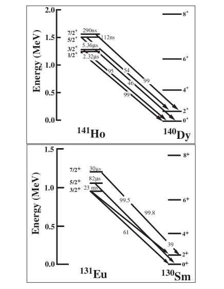
As has been previously mentioned, a significant benefit of working in the nonadiabatic formalism is the proper treatment of the ground-state rotational band in the daughter nucleus. This makes it possible to easily calculate the fine structure in the proton emission. The presence of the rotational band in the daughter nucleus also gives rise to rotational bands built upon $J=\Omega$ bandheads in the parent nucleus. In a previous work [15], we discussed a rotational band in ¹³¹Eu built upon the $J={\frac{3}{2}}^{+}$ level associated with the $[411]{\frac{3}{2}}$ Nilsson orbital. The spacing of the levels in the parent nucleus follow nicely the expected $J(J+1)$ spacing with the same moment of inertia parameter as assumed for the daughter nucleus. Small deviations from the $J(J+1)$ spacing result from the Coriolis coupling.

To verify that the calculated band structure indeed belongs to the same intrinsic Nilsson configuration, one can inspect the $K$-decomposition of each rotational level. This is done by using Eq. (23) to project the nonadiabatic wave functions onto adiabatic states with good $K$. For the $J$=${\frac{3}{2}}^{+}$ orbital in ¹³¹Eu, the $K$-decomposition is shown in Table II. It is seen that the $K$=${\frac{3}{2}}$ dominates, although there appear small admixtures of other $K$ components due to the Coriolis coupling. Note the presence of the $K$=${\frac{1}{2}}$ which is forbidden in the strong coupling limit.

spin($J$)	$K={\frac{1}{2}}$	$K={\frac{3}{2}}$	$K={\frac{5}{2}}$	$K={\frac{7}{2}}$
$3/2$	$0.0017$	$0.9972$
$5/2$	$0.0040$	$0.9894$	$0.0056$
$7/2$	$0.0095$	$0.9770$	$0.0013$	$1.77\times 10^{-5}$

TABLE II.: $K$-decomposition of the calculated band members of the $[411]{\frac{3}{2}}$ band in ¹³¹Eu. The $K\neq{\frac{3}{2}}$ components arise from the Coriolis coupling.

A very different picture arises for the $J$=${\frac{1}{2}}^{+}$ band built upon the $[411]{\frac{1}{2}}$ Nilsson orbital in ¹⁴¹Ho. Its low-lying band members, through $J$=${\frac{7}{2}}$, are shown in Fig. 7. In this case, we do not see the development of a strongly coupled band as in ¹³¹Eu, but rather two nearly degenerate decoupled signature partners. This comes about due to the large decoupling parameter for this orbital. Since ¹⁴¹Ho is well deformed, we can consider the Coriolis interaction as a perturbation in the strong coupling approximation. For a $K={\frac{1}{2}}$ band, first-order perturbation theory gives [32]

$$E^{J}_{{\frac{1}{2}}}=E^{0}_{{\frac{1}{2}}}+\frac{1}{2{\cal J}}\left\{J(J+1)-\frac{1}{4}+a_{d}(-)^{J+{\frac{1}{2}}}(J+{\frac{1}{2}})\right\},$$ (25)

where $a_{d}$ is the decoupling parameter. For a non-zero decoupling parameter, the $J+{\frac{1}{2}}$ odd levels are shifted against the $J+{\frac{1}{2}}$ even levels with a degeneracy setting in for $|a_{d}|=1$. From studies of well-deformed and super-deformed bands in odd-$Z$ rare-earth nuclei, bands built on the $[411]{\frac{1}{2}}$ level are known to have a decoupling parameter near $-1$ [43, 44]. This nicely explains our predictions and gives yet another verification that the weak coupling formalism properly incorporates the Coriolis interaction. It needs to be noted that the branchings shown in Fig. 7 correspond to the proton emission only. In reality, the low-lying levels in these bands rapidly decay by gamma radiation ($\Gamma_{\gamma}\gg\Gamma_{p}$); that is, the lifetimes of these states are much shorter.

FIG. 7.: Rotational bands in ¹³¹Eu (bottom; built upon the [411]3/2 Nilsson level) and ¹⁴¹Ho (top; built upon the [411]1/2 Nilsson level). For ¹³¹Eu, the strongly coupled rotational band is predicted. For ¹⁴¹Ho, the two decoupled, almost degenerate, sequences are calculated. Proton lifetimes and strongest branching ratios are indicated.

It is interesting to look in detail at the make-up of the cluster radial wave function and the partial widths. In the partial wave decomposition, the dominant components are those of the originating spherical state. For example, in ¹¹⁷La, the $[422]{\frac{3}{2}}$ Nilsson orbital originates from a $g_{7/2}$ spherical state. At a deformation of $\beta_{2}=0.33$, the wave function still contains $60\%$ of $g_{7/2}$ distributed between the $2^{+}$ and $4^{+}$ daughter states. However, due to deformation, other partial waves with $j\geq{\frac{3}{2}}$ also contribute: $d_{3/2}\,(9.6\%)$, $d_{5/2}\,(9.0\%)$, $g_{9/2}\,(14.2\%)$, and $i_{11/2}\,(3.5\%)$. Coriolis coupling introduces the $s_{1/2}$ partial wave with an amplitude of $4.2\%$. Although the radial wave function is a combination of components having different angular momentum, the decay branches are easy to understand. The total width is governed by the high penetrability of low-$l$ partial waves. In fact, $97\%$ of the width of this resonance is in the $d_{3/2}\otimes 0^{+}$ channel. The remaining part comes from the $d_{3/2}\otimes 2^{+}(0.6\%)$ and the $s_{1/2}\otimes 2^{+}(2.3\%)$ channels.

The majority of decays investigated in this work have small branching ratios, less than ten percent. However, a few have quite large branching ratios to $2^{+}$ states, including the possible decay out of the $[532]{\frac{5}{2}}$ Nilsson orbital in ¹³¹Eu which is predicted in this work to have the branching ratio of 52%. The circumstances that lead to such large branching ratios are worthy of investigation. The $[532]{\frac{5}{2}}$ orbital originates from an $h_{11/2}$ spherical orbital. At a deformation of $\beta_{2}=0.32$, the $[532]{\frac{5}{2}}$ orbital consists mainly of $h_{11/2}(75\%)$, $f_{7/2}(18\%)$ and only $1.9\%$ of $f_{5/2}$. There is an additional $0.8\%$ of the $K$-forbidden $p_{3/2}$ component. The decay to the ground state can proceed only via the $f_{5/2}$ component. Meanwhile, the decay to the $2^{+}$ state proceeds mainly through the $p_{3/2}$ and $f_{7/2}$ waves; the former due to the lower angular momentum and the latter due to the larger make-up in the total wave function. The combination of a low-lying excited state, a lower angular momentum channel, and suppressed amplitude of the $f_{5/2}$ wave leads to the very high branching ratio this state would exhibit.

B Branching Ratios

The main impetus behind this work has been the recently observed fine structure in the proton decay of ¹³¹Eu [7]. The nonadiabatic formalism offers great advantages over the strong-coupling approximation in calculating fine structure. The proper placement of the daughter states are explicitly included and the channels are now labeled with the proton’s orbital and total angular momentum, $lj$, and the angular momentum of the daughter nucleus, $J_{d}$. In one fell swoop, both the lifetime and partial widths are calculated.

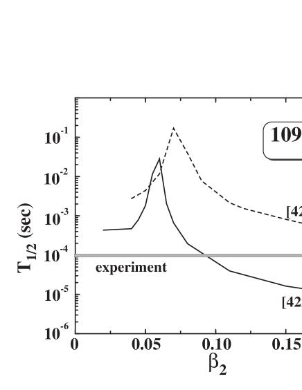
As was shown previously in Refs. [5, 15], for large deformations our calculations show little sensitivity to $\beta_{2}$ and $\beta_{4}$. This is because the spherical decomposition of the corresponding Nilsson orbitals varies little in this regime, provided that there are no crossings between the Nilsson orbitals of interest. The uncertainty due to nuclear deformation is usually smaller than that due to experimental uncertainty in the proton energy. In the less-deformed cases, there is a greater dependence of $\beta_{2}$ and $\beta_{4}$. In the $1/2^{+}$ level in ¹⁰⁹I, shown in Fig. 8, we see the effect of a level crossing near $\beta_{2}\approx 0.05$. (This effect has been noted earlier in Ref [13].)

FIG. 8.: Predicted lifetimes in ¹⁰⁹I for the [422]3/2 and [420]1/2 orbitals. The experimental lifetime is $110(5)\mu$s [38].

	Orbital	$u^{2}$	$\tau_{1/2}$	b.r.
109I	$[420]{\frac{1}{2}}$	0.99	94.8 $\mu$s	0%
	$[422]{\frac{3}{2}}$	0.99	7.86 ms	0%
			$110(5)\mu s$ [38]
113Cs	$[420]{\frac{1}{2}}$	0.52	0.66 $\mu$s	0%
	$J=3/2^{+}$	0.56	34.7 $\mu$s	0%
			$16.7(7)\mu s$ [4]
117La	$[420]{\frac{1}{2}}$	0.32	1.27 ms	0%
	$[422]{\frac{3}{2}}$	0.33	103 ms	3%
	$[541]{\frac{3}{2}}$	0.61	293 ms	4%
			20(5) ms [42]
131Eu	$[411]{\frac{3}{2}}$	0.71	34.0 ms	39%
	$[413]{\frac{5}{2}}$	0.52	184 ms	7%
	$[532]{\frac{5}{2}}$	0.48	3.90 s	52%
			17.8(19) ms	24(5)% [7]
141Ho	$[411]{\frac{1}{2}}$	0.70	14.6 $\mu$s	0.8%
	$[523]{\frac{7}{2}}$	0.84	19.1 ms	6%
			3.9(5) ms [5]
141mHo	$[411]{\frac{1}{2}}$	0.70	3.3 $\mu$s	1%
	$[523]{\frac{7}{2}}$	0.84	4.6 ms	9%
			$8(3)\mu s$ [5]

TABLE III.: Table showing the various orbitals for each system investigated in this work. Except for the weakly deformed systems of ¹⁰⁹I and ¹¹³Cs, the deformation dependence is much weaker than the uncertainty due to the experimental $Q_{p}$ value. The theoretical spectroscopic factor, half-life, and branching ratio to the $2^{+}$ states are shown. Experimental results (where available) are shown in bold type.

Table III shows predicted half-lives, theoretical spectroscopic factors, and branching ratios. The spectroscopic factors have been estimated in the independent-quasi-particle picture. Note that the $1/(\Omega+{\frac{1}{2}})$ factor present in the strong-coupling approximation is no longer needed. Our predictions for ¹³¹Eu and the ground and isomeric states in ¹⁴¹Ho are unchanged from [15]. The ground state of ¹³¹Eu is consistent with the $[411]{\frac{3}{2}}$ assignment. This is the same conclusion as in Refs. [7, 21] but differs from the assignment of $[413]{\frac{5}{2}}$ of Ref. [13].

In ¹⁴¹Ho, the assignments are straightforward: $[523]{\frac{7}{2}}$ for the ground state and $[411]{\frac{1}{2}}$ for the isomeric state. These match the assignments of Refs. [3, 13]. In ¹⁰⁹I we find agreement with the $[420]{\frac{1}{2}}$ with a deformation near $\beta_{2}$=0.10. This agrees with suggestions of Refs. [9, 13]. In ¹¹³Cs we see a large admixture of $K$=1/2 in the $J$=3/2 wave function. Therefore, the asymptotic Nilsson labeling is inappropriate, and only the total angular momentum is used to label the state in Table III. The two orbitals near the Fermi level in ¹¹³Cs correspond to a pseudospin doublet; hence, strong Coriolis mixing of these levels. In the newly discovered proton emitter ¹¹⁷La, the experimental lifetime is 20(5) ms [42]. It appears that the $[422]{\frac{3}{2}}$ assignment is best with a lifetime of 100 ms at a deformation of $\beta_{2}$=0.30, $\beta_{4}$=0.11.

FIG. 9.: Predicted half-lives for ¹³⁷Tb as a function of proton $Q_{p}$ value. The assumed deformation is $\beta_{2}=0.28$ and the estimated value of $E_{2^{+}}$ is $165$ keV. This figure is meant to identify the regions of $Q_{p}$ and $T_{1/2}$ to look for this yet-unseen proton emitter. For longer lifetimes, serious competition from beta decay is expected. Above the grey line, the branching ratio for proton decay is predicted to be less than $10\%$ [45].

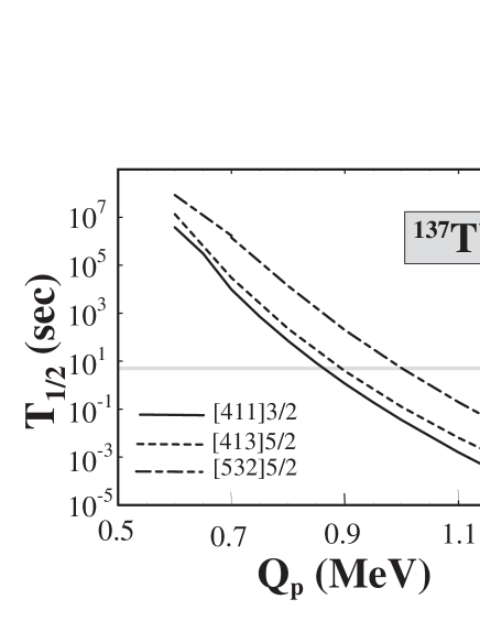
There is currently a proposal [46] to search for proton emission from ¹³⁷Tb. Being in the region between ¹³¹Eu and ¹⁴¹Ho, this nucleus is expected to be well deformed with $\beta_{2}$$\approx$0.28. Using the Grodzins formula [47, 48], we estimate the energy of the $2^{+}$ state in ¹³⁶Gd to be $165$ keV. Figure 9 shows the expected half-life as a function of $Q_{p}$. It is expected that for lifetimes longer than the limit marked by the grey line, beta-decay will dominate [46].

C Theoretical Uncertainties

It should be emphasized that our method contains no adjustable parameters; there are a few parameters which are set by experiment. These include $Q_{p}$ and the placement of the lowest few levels in the ground-state band of the daughter nucleus. Since the higher levels are energetically forbidden, even if they are needed in the calculation to ensure proper convergence, the half-lives and branching ratios are fairly insensitive to their placement. We shall now discuss the sensitivity of the calculated half-lives and branching ratios to various quantities used in the calculations. For concreteness, we will focus on the $[411]{\frac{3}{2}}$ level in ¹³¹Eu. All other levels studied show similar sensitivities.

The largest effect on the lifetime comes from the $Q_{p}$ value. The $Q_{p}$ value for ¹³¹Eu is currently taken as 950(7) keV [7]. The uncertainty of 7 keV leads to an uncertainty in the calculated lifetime of $-7.5/+9.8$ ms. This is a difference of roughly $-22/+30\%$. Since a change in the $Q_{p}$ value also affects the energies of excited states, the change in branching ratio is much smaller. For the $[411]{\frac{3}{2}}$ orbital, the effect is $\pm 1.3$ %.

On the other hand, the placement of the $2^{+}$ level has a smaller effect on the lifetime but greatly influences the branching ratio. Based on Ref. [7], the $2^{+}$ level in ¹³⁰Sm is placed at 121(7) keV. This 7 keV uncertainty changes the lifetime by $\pm 4.0$ ms ($\pm 12\%$). For the branching ratio, the corresponding error is $\pm 6.7$%.

In the nuclei with significant branching ratios, little to nothing is known about the level structure in the daughter system; hence, we had to assume a perfect rotor to assign energies to the states above the $2^{+}$. To check for the sensitivity to this assumption, we repeated some calculations assuming $E_{J_{d}}=\kappa^{\prime}J_{d}(J_{d}+1)-B[J_{d}(J_{d}+1)]^{2}$. The anharmonicity factor, $B$, has typical values around $\kappa^{\prime}/200\approx 100$ eV [49]. This introduces a 1.0 ms shortening of the lifetime and a reduction of the branching ratio of 1.2%. Both are much smaller than the influence of the $Q_{p}$ value or $E_{2^{+}}$. So as long as the proper $Q_{p}$ value is used along with a good estimate of the first excited state, the remaining part of the spectrum needs only to be reasonably placed.

Additional uncertainties can arise from the optical model potentials. As discussed in Sec. II C, we believe that the Chepurnov parameterization is the best current compromise. (It is noted here that better agreement between theory and experiment could, in principle, be achieved by fitting the optical model parameters to the properties, including proton decay data, of these drip-line nuclei.) As discussed in Ref. [8], the lifetime of spherical proton emitters depends weakly on the nuclear structure details. Reasonable variations in radius and diffuseness parameters affect the lifetimes by less than a factor of about three.

V Assessment of the adiabatic approximation

As discussed in Sec II, all previous work on deformed proton emitters have made the adiabatic approximation (AD) [3, 5, 7, 9, 11, 12, 13, 14, 20, 21]. The use of the nonadiabatic formalism for proton emission was first used by us in the recent Ref. [15]. The power of the nonadiabatic approach is apparent in several areas. First, due to the fact that the wave function is in the laboratory frame, the Coriolis coupling is implicitly included. This allows for the inclusion of all the partial waves with $j<J$ in the proton’s wave function. In particular, the Coriolis coupling can admix states with smaller $l$-values, and consequently lower centrifugal barriers, into the proton wave function. Low-$l$ components, however small, can substantially affect the lifetime.

FIG. 10.: Comparison of partial widths and wave function amplitudes obtained in the nonadiabatic (left) and adiabatic (right) calculations for the $[532]{\frac{5}{2}}$ deformed resonance in ¹³¹Eu. Only the lowest few partial waves are shown. The upper panels show the spherical amplitudes $|c_{\alpha}|^{2}$. Notice the presence of the $K$-forbidden $p$-wave components in the nonadiabatic approach. The lower panel shows the normalized partial widths $\gamma_{\alpha}\equiv\Gamma_{\alpha}/\Gamma_{\rm tot}$. In the non-adiabatic case we have summed over all possible daughter states.

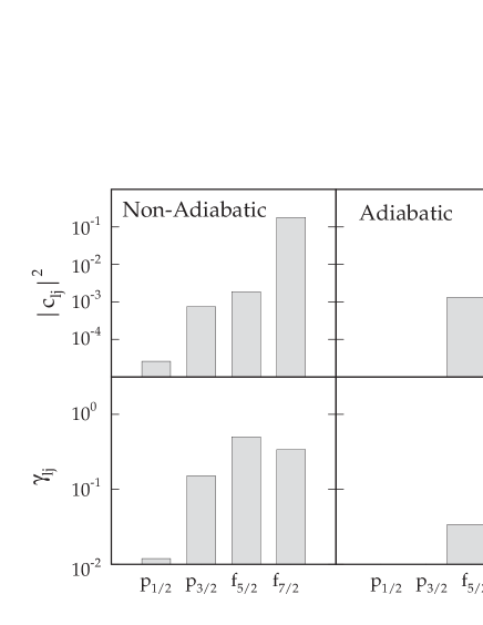
Figure 10 shows this effect for the $[532]{\frac{5}{2}}$ deformed resonance in ¹³¹Eu. Note that the $p_{3/2}$ partial wave contributes only $0.3\%$ to the total wave function, yet accounts for $15\%$ of the decay width.

In order to calculate the branching ratio in the adiabatic approximation, some ansatz must be used. Firstly, the partial width to the ground state is approximated by the width for the partial wave that matches the initial state,

$$\Gamma_{0^{+}}^{\rm ad}=\frac{1}{\Omega+{\frac{1}{2}}}\Gamma_{lj=\Omega}^{\rm ad}.$$ (26)

For the excited states, a weighted sum over the possible partial wave components is used:

$$\Gamma_{J_{d}}^{\rm ad}=\frac{2J_{d}+1}{\Omega+{\frac{1}{2}}}\sum_{lj}\,|\langle J_{d}0\;j\Omega|\Omega\Omega\rangle|^{2}\;\;\Gamma_{lj}^{\rm ad}(Q_{J_{d}}),$$ (27)

where the partial widths have been calculated with a $Q_{p}$ value adjusted to that of the $J_{d}^{+}$ state. This reduces to Eq. (26) for $J_{d}=0$. This procedure will be referred to as the adiabatic corrected method (ADC).

Nucleus	Orbital	$\tau_{{\frac{1}{2}}}$ (AD)	$\tau_{{\frac{1}{2}}}$ (ADC)	b.r.
109I	$[420]{\frac{1}{2}}$	$9.85\times 10^{-6}$	$24.1\times 10^{-6}$	0%
113Cs	$J=3/2^{+}$	$1.98\times 10^{-6}$	$7.02\times 10^{-6}$	0%
117La	$[422]{\frac{3}{2}}$	$20.5\times 10^{-3}$	$90.3\times 10^{-3}$	0.3%
131Eu	$[411]{\frac{3}{2}}$	$868.\times 10^{-6}$	$48.7\times 10^{-3}$	37%
141Ho	$[523]{\frac{7}{2}}$	$5.95\times 10^{-3}$	$6.66\times 10^{-3}$	3%
141mHo	$[411]{\frac{1}{2}}$	$1.94\times 10^{-6}$	$3.43\times 10^{-6}$	1%

TABLE IV.: A calculation of the proton lifetimes using the adiabatic formalism of Sec. II B. All lifetimes are in seconds. The label (AD) corresponds to calculations in the adiabatic approximation, i.e., it includes all degenerate final states. The column ADC corresponds to the corrected adiabatic approximation, in which it is assumed that the decay goes only to the ground state of the daughter nucleus, Eq. (26). The branching ratio is calculated using Eqs. (26) and (27). For the nonadiabatic model predictions, cf. Table III.

As can be seen in Table IV, in some instances the adiabatic and nonadiabatic predictions are very close, like for ^141mHo and ¹¹⁷La. However, in other cases the differences are striking, like the factor of five difference in ¹¹³Cs. In those systems where the agreement is good, there is no admixture of lower-$l$ partial waves in the nonadiabatic formalism.

It is also worth noting that lifetimes calculated in the full adiabatic method are usually shorter by a factor of up to four as compared to the ADC method. However, for the $[411]{\frac{3}{2}}$ orbital of ¹³¹Eu, there is a factor of 56 difference. This results from the large $J_{d}^{\pi}$=$2^{+}$ component in the corresponding Nilsson model function.

In about half of the cases studied, the adiabatic approximation, particularly with angular momentum conservation enforced by hand, gives results similar to the nonadiabatic method. In the rest, the difference can be large.

VI Conclusions

The state-of-the-art coupled-channel formalism has been extended to include excitation modes in the daughter system. The weak-coupling scheme applied allows us to work in the laboratory reference frame. The exact treatment of excitation spectrum in the daughter nucleus also allows a consistent calculation of branching ratios.

As could be expected, significant branching ratios are expected only for well-deformed nuclei where the first excited state of the daughter nucleus lies low in energy. The Coriolis mixing of states with lower orbital angular momentum can enhance the decay to the excited state, e.g., the decay of the $[532]{\frac{5}{2}}$ orbital in ¹³¹Eu where the branching ratio to the $2^{+}$ state is predicted to be as large as $52\%$.

In the case of spherical proton emitters, the proton separation energy and orbital angular momentum have the largest effect on lifetimes [8]. The detailed nuclear structure plays a minor role. In the deformed case, the placement of the single-particle levels also has a significant effect. This is true in both the adiabatic formalism, where mixing occurs with higher-$l$ states, and in the nonadiabatic formalism where the Coriolis coupling can mix states with lower-$l$ also.

We have been able to calculate the placement and decay properties of excited levels in the ground-state band of the parent nucleus. As shown in Fig. 7, both strongly coupled and nearly degenerate decoupled bands are predicted, depending on the nature of the band head. While we have calculated the proton decay half-lives of the excited band members, they are all much too slow to compete with in-band gamma-decay. In all cases investigated, by comparing theoretical predictions with experimental half-lives and branching ratios (where available), we have been able to identify the Nilsson orbital which the proton occupies. We have also been able to discern the angular momentum components of the proton wave function.

While our calculations for well-deformed nuclei give a quantitative agreement with experiment, it would not be proper to apply the present model to vibrational or transitional nuclei such as ¹⁵¹La. For this, one needs to redefine the coupling matrix elements in Eq. (7). Calculations along these lines are in progress.