Extra dimensions, SN1987a, and nucleon-nucleon scattering data

Abstract

One of the strongest constraints on the existence of large, compact, “gravity-only” dimensions comes from SN1987a. If the rate of energy loss into these putative extra dimensions is too high, then the neutrino pulse from the supernova will differ from that actually seen. The dominant mechanism for the production of Kaluza-Klein gravitons and dilatons in the supernova is via gravistrahlung and dilastrahlung from the nucleon-nucleon system. In this paper we compute the rates for these processes in a model-independent way using low-energy theorems which relate the emissivities to the measured nucleon-nucleon cross section. This is possible because for soft gravitons and dilatons the leading contribution to the energy-loss rate is from graphs in which the gravitational radiation is produced from external nucleon legs. Previous calculations neglected these mechanisms. We re-evaluate the bounds on toroidally-compactified “gravity-only” dimensions (GODs), and find that consistency with the observed SN1987a neutrino signal requires that if there are two such dimensions then their radius must be less than 1 micron.

I Introduction

The conjecture that the four-dimensional universe we perceive is merely a projection of a higher-dimensional space dates back at least to the work of Kaluza and Klein in the 1930s. Such ideas imply that we live in a world in which there are four infinite dimensions, and $n$ compactified “extra” dimensions. If this is the case there is the possibility of observing Kaluza-Klein (KK) modes, which correspond to excitations of ordinary standard-model particles in these extra dimensions. The absence of any such effects in collider experiments performed to date then places stringent limits on the size of such extra dimensions, forcing them to have inverse radii larger than $1~{}{\rm TeV}$ [1]. Until ten years ago the conventional wisdom was that the size of these extra dimensions would be set by the Planck mass, and so would be much smaller than this.

In the last decade this conventional wisdom has been under attack from two different, but connected, directions. Firstly, it has been suggested that string theory could lead to compactified dimensions which have radii much larger than $1/M_{P}$ [2, 3, 4]. Secondly, an alternative picture of the extra dimensions has emerged, in which the standard-model fields are confined to a four-dimensional “brane”, while gravity propagates in the $(n+4)$-dimensional “bulk”. This has generated considerable excitement because it seems to provide a natural solution to the hierarchy problem. Effectively, gravity is much weaker than the three other forces because it is diluted via its propagation in the extra dimensions. One simple scenario in which this occurs was suggested by Arkani-Hamed et al. [5, 6, 7]. Suppose that there are $n$ compact “gravity-only” dimensions (GODs) whose radius $R$ is large compared to the scale of fundamental physics in the $(n+4)$-dimensional world, $M_{(4+n)}$. For distances $r\gg R$, the gravitational force will behave like [6]:

$$F=\frac{1}{M_{(4+n)}^{\,\,n+2}}\frac{1}{4\pi R^{n}}\frac{m_{1}m_{2}}{r^{2}},$$ (1)

where $M_{(4+n)}$ is the fundamental scale of gravity in the $(n+4)$-dimensional world. Matching to the Newtonian law of gravity, which is the effective theory for long distances and weak fields, we see that

$$4\pi G_{N}=\left(\frac{1}{RM_{(4+n)}}\right)^{n}\frac{1}{M_{(4+n)}^{\,\,2}},$$ (2)

and so if $R\gg 1/M_{(4+n)}$ then the effective four-dimensional Planck scale $M_{P}\sim 1/\sqrt{G_{N}}$ will be much larger than the underlying $(n+4)$-dimensional scale $M_{(4+n)}$.

Of course, at distances $r\sim R$ the inverse-square law begins to break down. Choosing $M_{(4+n)}\sim 1$ TeV implies, for a given $n$, a definite value of the scale $R$ at which this breakdown occurs. In the case $n=1$ gravity would be modified on solar-system distance scales, but for $n=2$ the distance $R$ is already smaller than 1 mm. Thus, while the case of one GOD is ruled out experimentally, no direct measurement of gravity has, as yet, been made that precludes the existence of more than one GOD [6].

An alternative to measuring the gravitational force at distances of order one millimetre is to perform collider physics searches at the scale $M_{(4+n)}$ and look for “physics beyond the standard model” [9, 10, 11]. It is not immediately apparent that such searches will reveal any phenomenologically-significant effects. The only modification to physics at the scale $M_{(4+n)}$ is in the physics of gravity, and so the violations of the standard model appearing at that scale are, naively, only of gravitational strength. However, at such energies a large number of graviton KK modes are excited, even though all standard-model fields continue to behave as four-dimensional objects. This compensates for the weak coupling between these KK modes and matter fields. Production of KK-gravitons, $h$, and KK-dilatons, $\phi$, as well as their virtual contributions lead to deviations from the predictions of the standard model, as demonstrated in Refs. [9, 10, 11]. It is possible that such deviations could be detected at future colliders [12, 13].

Significant constraints have already been placed on the size of compact GODs from precision experiments at existing colliders [14]. However, these collider bounds are not the most stringent ones on the size of these dimensions. Arkani-Hamed et al. pointed out that one of the strongest bounds on this physics comes from SN1987a [6]. The argument is very similar to that used to bound the axion-nucleon coupling strength [15, 16, 17, 18]. The “standard model” of supernovae does an exceptionally good job of predicting the duration and shape of the neutrino pulse from SN1987a. Any mechanism which leads to significant energy-loss from the core of the supernova immediately after bounce will produce a very different neutrino-pulse shape, and so will destroy this agreement—as demonstrated explicitly in the axion case by Burrows, Brinkmann, and Turner [17]. Raffelt has proposed a simple analytic criterion based on detailed supernova simulations [18]: if any energy-loss mechanism has an emissivity greater than $10^{19}$ ergs/g/s then it will remove sufficient energy from the explosion to invalidate the current understanding of Type-II supernovae’s neutrino signal. In the case of interest here the bremsstrahlung processes ${NN\rightarrow NNh}$ (KK-gravistrahlung) and ${NN\rightarrow NN\phi}$ (KK-dilastrahlung), provide an energy-loss mechanism for the supernova. Energy generated during the collapse is radiated away into the extra-dimensional degrees of freedom, never to return. Demanding that such reactions do not result in the loss of too much energy from the supernova allows bounds to be placed on the size of the toroidally-compactified GODs.

Two attempts to place such a constraint have already appeared in the literature [19, 20]. Both assumed that the $NN$ scattering amplitude was dominated by a single virtual pion exchange—an uncontrolled approximation which we refer to hereafter as “the one-pion-exchange approximation”. Although this approximation appears reasonable, since one-pion exchange is the long-distance component of the nuclear force, in fact the nuclear physics of this problem is much more complicated. Most obviously, the very existence of nuclei tells us that the strong nuclear force is non-perturbative. Yet, the calculations of Refs. [19, 20] are only valid if one-pion exchange can be treated in Born approximation. Hence, the $NN$ interactions which occur during these radiative processes should, instead, be described by the full $NN$ t-matrix.

One might think that such a calculation is model-dependent and complicated. However, in the limit that the emitted radiation is soft compared to the incoming $NN$ energy, the calculation simplifies dramatically. In this limit there are low-energy theorems for the emission of radiation which are analogous to those for photon bremsstrahlung [21, 22]. These theorems relate the amplitude for the bremsstrahlung process to the on-shell $NN$ amplitude. It thus becomes possible to use $NN$ scattering data to calculate low-energy emission processes directly. Recently, three of the present authors used theorems of this sort for axial bremsstrahlung to perform a more reliable calculation of axion and neutrino bremsstrahlung in a nucleon gas [23]. The resultant rates are model-independent, and rely only on two assumptions: that the radiation is soft, and that the emission rate from the nuclear gas is dominated by two-body collisions. The use of such an approach therefore essentially eliminates the two-body dynamics as a source of uncertainty in the problem.

In this paper we will derive model-independent low-energy theorems which relate the amplitudes for ${NN\rightarrow NNh}$ and ${NN\rightarrow NN\phi}$ to the on-shell $NN$ scattering amplitude. It turns out that at both leading and next-to-leading order (LO and NLO) in the soft expansion the cross sections for these production processes can be expressed directly in terms of the $NN$ differential cross section. We use the NLO production cross sections to compute the energy loss from a supernova due to KK-graviton and KK-dilaton radiation from the two-nucleon system. The “Raffelt criterion” explained above then leads directly to a constraint on the size of the extra dimensions.

The paper proceeds as follows. In Section II we derive the amplitude for the emission of soft gravitational radiation from the $NN$ system. We include all terms which contribute up to the first two orders in the soft expansion. We then take the amplitude at NLO in the soft expansion and use it to compute the energy loss due to the three processes ${NN\rightarrow NNh}$, ${NN\rightarrow NN\phi}$, and $NN\rightarrow NNg$, where $g$ is the four-dimensional graviton. In Section III we derive formulae, meant for numerical evaluation, which yield the emissivity of a gas of nucleons due to these production mechanisms, give our “best” result for the bound on the size of the extra dimensions, and discuss the validity of the soft approximation. Section IV then examines the limiting cases of non-degenerate and degenerate neutron matter. In these limits analytic formulae for the emissivity in terms of a single $NN$ cross section may be obtained. We also exhibit the analytic formulae found if one assumes that effective-range theory describes the $NN$ cross section, and present the radius bounds given by these analytic calculations. Finally, Section V presents the results for the supernova emissivity obtained with all of these different approaches, and compares and contrasts them with the work of Refs. [19, 20].

Many-body effects, although undoubtedly important, were not the focus of Ref. [23], and will not be part of our discussion here. While the radiation from the two-body system can be computed in a model-independent way, the evaluation of many-body effects is necessarily model-dependent, since it relies on selective re-summations of classes of diagrams in the many-body problem. One set of many-body effects which can modify the vacuum rates for KK-graviton emission was considered in Ref. [24]. We look forward to future work on how many-body physics affects the reactions ${NN\rightarrow NNh}$ and ${NN\rightarrow NN\phi}$, but we have not focused on these issues here, since our goal was to provide a firm, model-independent, foundation on which future calculations of many-body corrections to these processes can build.

II ${NN\rightarrow NNh}$ and ${NN\rightarrow NN\phi}$

A Graviton and dilaton dynamics in $n+4$ dimensions

For simplicity, we let the $n$ extra dimensions form an $n$-torus of radius $R=L/(2\pi)$ in each direction. The zero-modes of the $(n+4)$-dimensional graviton correspond to the massless graviton, $h_{\mu\nu}$, the $(n-1)$ vector bosons $A_{\mu}$ (which decouple from the matter fields) and $n(n-1)/2$ scalar fields, $\phi_{\mu\nu}$. The graviton and scalar field mode expansions have the form

$$h^{\mu\nu}(x,\vec{y}^{\,}) = \sum_{\vec{j}}h^{\mu\nu,\vec{j}}(x)\ \exp\left(i{2\pi{\vec{j}}\cdot{\vec{y}}\over L}\right),\qquad\phi_{ab}(x,\vec{y}^{\,})=\sum_{\vec{j}}\phi^{\vec{j}}_{ab}(x)\ \exp\left(i{2\pi{\vec{j}}\cdot{\vec{y}}\over L}\right),$$ (3)

where $x$ are the 4-dimensional coordinates, $\vec{y}$ are the $n$-dimensional coordinates, and $\vec{j}$ is an $n$-dimensional vector representing the momentum of the mode in the extra dimensions. Although these modes are massless in the $(n+4)$-dimensional world this extra-dimensional momentum results in an effective mass on the four-dimensional brane, $m_{\vec{j}}$, with

$$m_{\vec{j}}^{2}={4\pi^{2}|{\vec{j}}|^{2}\over L^{2}}.$$ (4)

We use KK-graviton fields with polarization tensors $e^{\vec{j}}_{\mu\nu}(\vec{k},\lambda)$, where the extra-dimensional momentum is $\vec{j}$, while the graviton is propagating in the direction $\hat{k}$ in our world, and has polarization $\lambda$. Then

$$\sum_{\lambda=1}^{5}\ e^{\vec{j}}_{\mu\nu}(\vec{k},\lambda)\left[e^{\vec{j}}_{\rho\sigma}(\vec{k},\lambda)\right]^{*}\ =\ {1\over 2}B^{\vec{j}}_{\mu\nu,\rho\sigma}(\vec{k}),$$ (5)

with [9, 10]

$$B^{\vec{j}}_{\alpha\beta\mu\nu}=\left(\eta_{\mu\alpha}\eta_{\nu\beta}+\eta_{\mu\beta}\eta_{\nu\alpha}-\eta_{\nu\mu}\eta_{\alpha\beta}\right) - \frac{1}{m_{\vec{j}}^{2}}\left(\eta_{\mu\alpha}k_{\nu}k_{\beta}+\eta_{\nu\beta}k_{\mu}k_{\alpha}+\eta_{\mu\beta}k_{\nu}k_{\alpha}+\eta_{\nu\alpha}k_{\mu}k_{\beta}\right)$$ (6)

$$+ \frac{1}{3}\left(\eta_{\mu\nu}+\frac{2}{m_{\vec{j}}^{2}}k_{\mu}k_{\nu}\right)\left(\eta_{\alpha\beta}+\frac{2}{m_{\vec{j}}^{2}}k_{\alpha}k_{\beta}\right).$$ (7)

The Lagrange density that describes the four-dimensional interactions between the KK-graviton and KK-dilaton, and matter fields is then [9, 19]

$${\cal L} = -{\kappa\over 2}\sum_{\vec{j}}\left[\ h^{\mu\nu,\vec{j}}T_{\mu\nu}\ +\ \sqrt{2\over 3(n+2)}\phi^{\vec{j}}T^{\mu}_{\mu}\ \right],$$ (8)

where $T_{\mu\nu}$ is the conserved energy-momentum tensor of the matter on the 4-dimensional brane, and the dilaton field is $\phi=\phi_{aa}$. We have also defined $\kappa=\sqrt{32\pi G_{N}}$, with $G_{N}$ being Newton’s gravitational constant.

B Radiation from the $NN$ system in the soft limit

To compute gravitational radiation from the $NN$ system we must calculate the energy-momentum tensor of free nucleons. Neglecting isospin violation in the strong interaction, and electroweak effects

$$T_{\mu\nu}^{N} = {i\over 2}\overline{\psi}\left(\overrightarrow{\partial}_{\mu}-\overleftarrow{\partial}_{\mu}\right)\gamma_{\nu}\psi-g_{\mu\nu}{\cal L}\ \rightarrow\ -{1\over 4M}\overline{\psi}\left(\overrightarrow{\partial}_{\mu}-\overleftarrow{\partial}_{\mu}\right)\left(\overrightarrow{\partial}_{\nu}-\overleftarrow{\partial}_{\nu}\right)\psi\ +\ ...\ \ \ ,$$ (9)

where the ellipses denote spin-dependent interactions that do not contribute if the momentum of the emitted radiation is small, and terms that can be made to vanish by the nucleon equations of motion. $M$ is the isospin-averaged nucleon mass. This, together with Eq. (8), defines the leading interaction between a single KK-graviton or KK-dilaton and a nucleon.

FIG. 1.: The leading diagrams contributing to processes ${NN\rightarrow NNh}$ and ${NN\rightarrow NN\phi}$. Nucleons are denoted by solid lines and the KK-modes $h$ or $\phi$ are denoted by dashed lines. Solid squares denote an insertion of the single-nucleon energy-momentum tensor, while solid ovals containing ${\cal A}$ denote an insertion of the full $NN$ scattering amplitude. The solid oval containing $\Gamma$ denotes the non-pole vertex required for the sum of diagrams to satisfy $\partial_{\mu}M^{\mu\nu}=0$.

Now we fix our attention on the case of KK-graviton emission, and examine the limit when the emitted graviton is soft—which is to say its energy, $\omega$, is much less than all other scales in the problem. This means that we certainly want $\omega\ll p^{2}/M$, the incoming energy of the $NN$ system, although other restrictions will also emerge, as we shall see below. In what follows we shall treat $\omega M/p^{2}$ as a small, dimensionless, expansion parameter, and compute the contribution of the first two orders in this expansion to the amplitude for ${NN\rightarrow NNh}$.

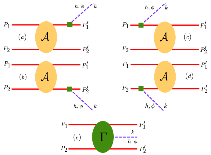
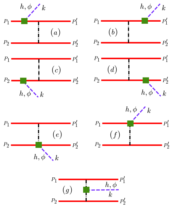
In the limit $\omega M/p^{2}\ll 1$ the amplitude for gravistrahlung is dominated by graphs (a)–(d) in Fig. 1. In Fig. 1 the incoming nucleon momenta are $p_{1}$, $p_{2}$, the outgoing nucleon momenta are $p_{1}^{\prime}$, $p_{2}^{\prime}$, and the KK-graviton four-momentum is denoted by $k$. We must also define Mandelstam variables $s_{i}$ and $s_{f}$ for the $NN$ interaction, depending on whether the nucleons scatter before or after the graviton emission. Likewise, two different Mandelstam $t$’s enter, depending on whether the KK-graviton is emitted from nucleon 1 or nucleon 2. Denoting

$$s_{i}=(p_{1}+p_{2})^{2};\qquad s_{f}=(p_{1}^{\prime}+p_{2}^{\prime})^{2}$$ (10)

$$t_{1}=(p_{1}-p_{1}^{\prime})^{2};\qquad t_{2}=(p_{2}^{\prime}-p_{2})^{2}.$$ (11)

The amplitudes for KK-graviton emission from the four graphs (a)–(d) may then be written as:

$$iM_{\mu\nu}^{(a)} = \left(\frac{-i\kappa}{8M}\right)(2p_{1}^{\prime}+k)_{\mu}(2p_{1}^{\prime}+k)_{\nu}\bar{u}(\vec{p_{1}}^{\prime})\bar{u}(\vec{p_{2}}^{\prime})\frac{i}{\not\!p_{1}^{\prime}+\not\!k-M}(-i){\cal A}(s_{i},t_{2})u(\vec{p_{1}})u(\vec{p_{2}}),$$ (12)

$$iM_{\mu\nu}^{(b)} = \left(\frac{-i\kappa}{8M}\right)(2p_{2}^{\prime}+k)_{\mu}(2p_{2}^{\prime}+k)_{\nu}\bar{u}(\vec{p_{1}}^{\prime})\bar{u}(\vec{p_{2}}^{\prime})\frac{i}{\not\!p_{2}^{\prime}+\not\!k-M}(-i){\cal A}(s_{i},t_{1})u(\vec{p_{1}})u(\vec{p_{2}}),$$ (13)

$$iM_{\mu\nu}^{(c)} = \left(\frac{-i\kappa}{8M}\right)\bar{u}(\vec{p_{1}}^{\prime})\bar{u}(\vec{p_{2}}^{\prime})(-i){\cal A}(s_{f},t_{2})\frac{i}{\not\!p_{1}-\not\!k-M}(2p_{1}-k)_{\mu}(2p_{1}-k)_{\nu}u(\vec{p_{1}})u(\vec{p_{2}}),$$ (14)

$$iM_{\mu\nu}^{(d)} = \left(\frac{-i\kappa}{8M}\right)\bar{u}(\vec{p_{1}}^{\prime})\bar{u}(\vec{p_{2}}^{\prime})(-i){\cal A}(s_{f},t_{1})\frac{i}{\not\!p_{2}-\not\!k-M}(2p_{2}-k)_{\mu}(2p_{2}-k)_{\nu}u(\vec{p_{1}})u(\vec{p_{2}}).$$ (15)

This amplitude begins at $O(\chi^{-1})$, with the small parameter $\chi$ is meant as a mnemonic for any of the quantities $|\vec{k}|$, $\omega$, and $m_{\vec{j}}$. The $u$’s are Dirac spinors, normalized so that $\bar{u}u=1$.

Note that here the amplitude ${\cal A}$ is the on-shell $NN$ amplitude projected onto positive-energy $NN$ states. One might think that is necessary to include in the expressions (12)–(15) the fact that one leg in the $NN$ interaction is off its mass shell. However, it is clear that the difference between using the on-shell $NN$ amplitude and the one that is “correct” for the kinematics of Fig. 1 is an $O(\chi^{0})$ effect. The low-energy theorem of Low [21] for $NN\rightarrow NN\gamma$, and that of Adler and Dothan [22] for axial bremsstrahlung, are both based upon the idea that we can construct the leading-order bremsstrahlung amplitude using the on-shell $NN$ amplitude, and then determine the terms of $O(\chi^{0})$ using current conservation. As we shall see below, a similar low-energy theorem exists in this case, and so we need not bother to include the off-mass-shell dependence of the $NN$ amplitude in Eqs. (12)–(15). In fact, in general the off-shell dependence of the $NN$ amplitude is the result of a particular choice for the nucleon interpolating field, and so it can always be changed by field redefinitions. S-matrix elements are unaffected by such field transformations [25].

We now simplify the above expression, by using the fact that ${\cal A}$ is projected onto positive-energy states, and retaining only the spin-independent terms up to $O(\chi^{0})$. Although it is possible to keep track of the spin-dependent terms, we will drop them here, since they always appear at $O(\chi^{0})$, and so, after summing over nucleon spins, do not make a contribution to the production cross section until $O(\chi^{0})$. This is two powers of $\chi$ beyond the leading term in the cross section. Thus, excluding these terms, the result is:

$$M_{\mu\nu}^{(a)} = -\frac{\kappa}{4}(2p_{1}^{\prime}+k)_{\mu}(2p_{1}^{\prime}+k)_{\nu}\frac{1}{2p_{1}^{\prime}\cdot k+k^{2}}\left(1+\frac{1}{2M^{2}}k\cdot p_{1}^{\prime}\right){\cal A}(s_{i},t_{2});$$ (16)

$$M_{\mu\nu}^{(b)} = -\frac{\kappa}{4}(2p_{2}^{\prime}+k)_{\mu}(2p_{2}^{\prime}+k)_{\nu}\frac{1}{2p_{2}^{\prime}\cdot k+k^{2}}\left(1+\frac{1}{2M^{2}}k\cdot p_{2}^{\prime}\right){\cal A}(s_{i},t_{1});$$ (17)

$$M_{\mu\nu}^{(c)} = \frac{\kappa}{4}{\cal A}(s_{f},t_{2})\left(1-\frac{1}{2M^{2}}k\cdot p_{1}\right)\frac{1}{2p_{1}\cdot k-k^{2}}(2p_{1}-k)_{\mu}(2p_{1}-k)_{\nu};$$ (18)

$$M_{\mu\nu}^{(d)} = \frac{\kappa}{4}{\cal A}(s_{f},t_{1})\left(1-\frac{1}{2M^{2}}k\cdot p_{2}\right)\frac{1}{2p_{2}\cdot k-k^{2}}(2p_{2}-k)_{\mu}(2p_{2}-k)_{\nu},$$ (19)

where we have also used the fact that the external nucleon legs are on-shell.

C Conserved $M_{\mu\nu}$

Observe that if we sum graphs (a)–(d) to get $M_{\mu\nu}$ then the result is not a conserved quantity. To remedy this, we generalize the prescription used in photon bremsstrahlung [21, 22], writing:

$$k^{\mu}M_{\mu\nu}=-k^{\mu}\Gamma_{\mu\nu}+O(\chi^{2}),$$ (20)

and then construct

$$M^{(0)}_{\mu\nu}=M_{\mu\nu}+\Gamma_{\mu\nu}.$$ (21)

By the same arguments that apply in the case of the Low [21] and Adler-Dothan [22] theorems, $M_{\mu\nu}^{(0)}$ will be the correct amplitude up to spin-dependent pieces of order $\chi^{0}$ and spin-independent pieces of $O(\chi^{1})$ .

A brief calculation then reveals that the spin-independent piece of the amplitude for $NN\rightarrow NNh$ is, up to $O(\chi^{0})$:

$$M_{\mu\nu}^{(0)} = \frac{\kappa}{4}\left[{\cal A}(s_{f},t_{2})\frac{1}{2p_{1}\cdot k-k^{2}}\left(2p_{1}-k\right)_{\mu}\left(2p_{1}-k\right)_{\nu}+{\cal A}(s_{f},t_{1})\frac{1}{2p_{2}\cdot k-k^{2}}\left(2p_{2}-k\right)_{\mu}\left(2p_{2}-k\right)_{\nu}\right.$$ (22)

$$- \left(2p_{1}^{\prime}+k\right)_{\mu}\left(2p_{1}^{\prime}+k\right)_{\nu}\frac{1}{2p_{1}^{\prime}\cdot k+k^{2}}{\cal A}(s_{i},t_{2})-\left(2p_{2}^{\prime}+k\right)_{\mu}\left(2p_{2}^{\prime}+k\right)_{\nu}\frac{1}{2p_{2}^{\prime}\cdot k+k^{2}}{\cal A}(s_{i},t_{1})$$ (23)

$$+ 2\eta_{\mu\nu}{\cal A}(\bar{s},\bar{t})+4(p_{1}+p_{2})_{\mu}(p_{1}+p_{2})_{\nu}\left.\frac{\partial{\cal A}(s,\bar{t})}{\partial s}\right|_{s=\bar{s}}+\left.4(p_{2}-p_{2}^{\prime})_{\mu}(p_{2}-p_{2}^{\prime})_{\nu}\left.\frac{\partial{\cal A}(\bar{s},t)}{\partial t}\right|_{t=\bar{t}}\right].$$ (24)

The classical amplitude for the emission of gravitational radiation from a system of colliding particles was derived many years ago by Weinberg [26]. We may now recover this result by retaining only the $O(\chi^{-1})$ parts of Eq. (LABEL:eq:M0):

$$M_{\mu\nu}^{(-1)}=\frac{\kappa}{2}\sum_{j}\eta_{j}{p_{j}}_{\mu}{p_{j}}_{\nu}\frac{1}{p_{j}\cdot k}{\cal A}(\bar{s},\bar{t}),$$ (26)

where $j$, the particle index, runs from 1 to 4, with $j=1,2$ for incoming nucleons and $j=3,4$ for outgoing nucleons, and

$$\quad\eta_{j}=\left\{\begin{array}[]{cl}1&\hbox{if $j=1,2$}\\ -1&\hbox{if $j=3,4$};\end{array}\right.$$ (29)

$$\bar{s}=\frac{s_{i}+s_{f}}{2};\quad\bar{t}=\frac{t_{1}+t_{2}}{2}.$$ (30)

Weinberg’s derivation of Eq. (26) is entirely classical, which is not surprising, since the graphs that contribute to the amplitude only involve radiation from external legs, and so they correspond to classical bremsstrahlung from the gravitational charges accelerated during the $NN$ collision. It is also worth pointing out that the Weinberg result is only valid if the $NN$ t-matrix is slowly varying over the energy region of interest.

Next observe that the conservation of $M$—$k^{\mu}M_{\mu\nu}=0$—implies the following relations:

$$M_{0i} = -\frac{k^{j}}{\omega}M_{ji},$$ (31)

$$M_{00} = \frac{k^{i}k^{j}}{\omega^{2}}M_{ji}.$$ (32)

This obviates the necessity to actually calculate these “0” components. These relations may be formalized by defining the symbol $W_{\mu\nu ij}$ as follows:

$$W_{\mu\nu ij}=\eta_{i\mu}\eta_{j\nu}-\eta_{i\mu}\eta_{0\nu}\frac{k_{j}}{\omega}-\eta_{0\mu}\eta_{j\nu}\frac{k_{i}}{\omega}+\eta_{0\mu}\eta_{0\nu}\frac{k_{i}k_{j}}{\omega^{2}}.$$ (33)

If $M_{\mu\nu}$ is conserved then we need only calculate the space-space components of this tensor. Other portions can be generated via the relation:

$$M_{\mu\nu}=W_{\mu\nu ij}M^{ij}.$$ (34)

In particular, if we work in the centre-of-mass frame, then at leading order in the nucleon velocity the space-space components of $M_{\mu\nu}$ have a very simple form:

$$M_{ij}^{(-1)}={\cal A}(\bar{s},\bar{t})\frac{\kappa}{M\omega}\left[p_{i}p_{j}-p_{i}^{\prime}p_{j}^{\prime}\right].$$ (35)

This result differs from Eq. (LABEL:eq:M0) by relativistic corrections, which are suppressed by two powers of $p/M$. In addition, the next-to-leading order (NLO) amplitude (LABEL:eq:M0) contains corrections to Eq. (35) which are suppressed by $\omega/M$. Since $\omega\ll p^{2}/M$, by assumption, the expansion in $p/M$ is less convergent than the one in $\omega/M$.

If we continue to neglect these effects of order $p^{2}/M^{2}$ and $\omega/M$, then we can also write down a compact formula for the next-order correction to $M_{ij}$:

$$M_{ij}^{(0)}=\kappa\left[-\frac{1}{2}\delta_{ij}{\cal A}(\bar{s},\bar{t})+(p_{i}-p_{i}^{\prime})(p_{j}-p_{j}^{\prime})\left.\frac{\partial{\cal A}}{\partial t}(\bar{s},t)\right|_{t=\bar{t}}\right],$$ (36)

where, once again, we have chosen to work in the centre-of-mass frame.

Note that working only at leading order involves neglecting the pieces of the amplitude $M_{\mu\nu}$ corresponding to variations of the $NN$ t-matrix in the Mandelstam variables $s$ and $t$. This is clearly not a good approximation at low energies, where the $NN$ t-matrix varies rapidly. At higher energies the scale of variation of ${\cal A}$ can be thought of as $m_{\pi}$, the pion mass, and so we would also like to have $\omega\ll m_{\pi}$. In fact, this is probably a rather conservative estimate, since empirically the energy and angle-dependence of the $NN$ cross section is quite weak at these higher energies. However, a proper test of the convergence of the soft expansion is really required.

One obvious way to perform such a test is to compute the LO result (35) and then compare it to the result at NLO. In Section II E we will show that in fact the NLO correction vanishes, and so the LO amplitude (35) is more reliable than one might naively expect.

D Result for energy loss from the $NN$ system to leading order

In this Section we will compute the energy-loss for a given graviton KK-mode $\vec{j}$. In Section III we sum over all modes in order to compute the total rate of energy emission from a gas of nucleons.

The energy loss due to graviton emission into a given KK mode $\vec{j}$ is given by:

$$d\varepsilon_{h}^{\vec{j}}=\omega\frac{d^{3}k}{(2\pi)^{3}2\omega}\sum_{\lambda}\left[{M}^{\alpha\beta}e^{\vec{j}}_{\alpha\beta}(\vec{k},\lambda)\right]^{*}e^{\vec{j}}_{\mu\nu}(\vec{k},\lambda){M}^{\mu\nu}.$$ (37)

(Strictly speaking this is not an energy loss, since we need to multiply by the density of initial and final $NN$ states, however, throughout this section we employ this somewhat lax terminology.)

Using the symbol $W$, defined in Eq. (33), we may rewrite this as

$$d\varepsilon_{h}^{\vec{j}}=\frac{dk\,k^{2}}{4\pi^{2}}\frac{d\hat{k}}{4\pi}\frac{1}{2}M_{ij}W^{\mu\nu ij}B^{\vec{j}}_{\mu\nu\alpha\beta}W^{\alpha\beta kl}M_{kl},$$ (38)

where $B$ is defined by Eq. (7). Since $k^{\mu}W_{\mu\nu kl}=0$ by construction, only the pieces of $B$ proportional to $\eta$ symbols survive. After some calculation we see that:

$$\frac{1}{2}W_{\mu\nu ij}B^{\mu\nu\alpha\beta}W_{\alpha\beta kl}=\frac{1}{2}\left(\eta_{ik}\eta_{jl}+\eta_{il}\eta_{jk}-\frac{2}{3}\eta_{ij}\eta_{kl}\right)$$ (39)

$$\qquad+\frac{1}{2\omega^{2}}\left(\eta_{ik}k_{j}k_{l}+\eta_{jk}k_{i}k_{l}+\eta_{il}k_{j}k_{k}+\eta_{jl}k_{i}k_{k}-\frac{2}{3}(k_{i}k_{j}\eta_{kl}+k_{k}k_{l}\eta_{ij})\right)+\frac{2}{3\omega^{4}}k_{i}k_{j}k_{k}k_{l}.$$ (40)

At this point we may integrate over the final-state graviton direction $\hat{k}$, since at LO $M_{ij}$ does not depend on $\hat{k}$. This gives:

$$\frac{1}{2}\int\frac{d\hat{k}}{4\pi}\,W_{\mu\nu ij}B^{\mu\nu\alpha\beta}W_{\alpha\beta kl}=\frac{19}{90}(\delta_{ik}\delta_{jl}+\delta_{il}\delta_{jk})-\frac{1}{15}\delta_{ij}\delta_{lk}$$ (42)

$$\qquad+\frac{m_{\vec{j}}^{2}}{\omega^{2}}\left(\frac{11}{45}(\delta_{ik}\delta_{jl}+\delta_{il}\delta_{jk})-\frac{14}{45}\delta_{ij}\delta_{kl}\right)+\frac{m_{\vec{j}}^{4}}{\omega^{4}}\frac{2}{45}(\delta_{ik}\delta_{jl}+\delta_{il}\delta_{jk}+\delta_{ij}\delta_{kl}).$$ (43)

Using the LO $M_{\mu\nu}$, Eq. (35), we finally obtain the following energy loss per unit frequency interval, for radiation into a KK mode of given mass $m_{\vec{j}}$,

$$\frac{d\varepsilon_{h}}{d\omega}=\frac{k}{\omega}\frac{8G_{N}}{5\pi}\frac{4\overline{p^{2}}^{2}}{M^{2}}\sin^{2}\theta_{\rm cm}|{\cal A}|^{2}\left(\frac{19}{18}+\frac{11}{9}\frac{m_{\vec{j}}^{2}}{\omega^{2}}+\frac{2}{9}\frac{m_{\vec{j}}^{4}}{\omega^{4}}\right),$$ (44)

where $\theta_{\rm cm}$ is the centre-of-mass scattering angle: $\cos\theta_{\rm cm}=\hat{p}\cdot\hat{p^{\prime}}$, and $\overline{p^{2}}=(p^{2}+{p^{\prime}}^{2})/2$.

This argument can also be pursued for 4-dimensional gravitons, provided one modifies the polarization tensor $B$ appropriately. The result for energy-loss due to 4D-graviton emission is:

$$\frac{d\varepsilon_{g}}{d\omega}=\frac{8G_{N}}{5\pi}\frac{4\overline{p^{2}}^{2}}{M^{2}}\sin^{2}\theta_{\rm cm}|{\cal A}|^{2},$$ (45)

as derived by Weinberg [26]. Note that this is not the $m_{\vec{j}}\rightarrow 0$ limit of Eq. (44), since the 4D-graviton has fewer degrees of freedom, due to its 4D-masslessness. Note also that here, and in Eqs. (44) and (47), we have made the replacement

$$p^{4}+{p^{\prime}}^{4}-2p^{2}{p^{\prime}}^{2}\cos^{2}\theta_{\rm cm}\quad\longrightarrow\quad 2\overline{p^{2}}^{2}\sin^{2}\theta_{\rm cm},$$ (46)

in order to make contact with Ref. [26] and simplify the formulae. This corresponds to evaluating the energy of the $NN$ system at the point $\bar{s}$. The error introduced by this replacement is of order $M^{2}\omega^{2}$, and so is suppressed by two powers of $\chi$.

Meanwhile, the result for energy loss due to KK-dilaton emission is also obtained by an analogous argument. It is:

$$\frac{d\varepsilon_{\phi}}{d\omega}=\frac{k}{\omega}\frac{8G_{N}}{5\pi}\frac{4\overline{p^{2}}^{2}}{M^{2}}\sin^{2}\theta_{\rm cm}|{\cal A}|^{2}{2\over 9(n+2)}\left(1-\frac{m_{\vec{j}}^{2}}{\omega^{2}}\right)^{2}.$$ (47)

E Next-to-leading order calculation

These energy-loss rates represent the leading-order result, which we shall denote by $O(\chi^{-2})$. To calculate the correction to this energy-loss rate which arises at NLO we must contract the amplitude (35) with the correction (36). Since—at least in the non-relativistic limit—the space-space components of the NLO amplitude do not depend on the direction of the emitted radiation, we may use the steps (37)–(43) employed above to show that the piece of $\frac{d\varepsilon_{h}}{d\omega}$ which arises at $O(\chi^{-1})$ vanishes.

To do this we first note that the trace of $M^{(-1)}$ over its spatial components, $M^{(-1)}_{ii}$, is $O(\chi^{0})$. Therefore, since we are trying to compute pieces of $\frac{d\varepsilon_{h}}{d\omega}$ that are $O(\chi^{-1})$ we can neglect terms such as $M_{ii}M_{jj}$. It also follows that the contraction of the $\delta_{ij}$ piece of $M^{(0)}_{ij}$ with $M^{(-1)}_{kl}$ only produces pieces of the energy-loss rate that are of higher order than we are concerned with here.

A brief calculation then shows that the contraction of the piece of $M^{(0)}_{ij}$ proportional to $\frac{\partial{\cal A}}{\partial t}$ with $M^{(-1)}_{kl}$ also only yields pieces of $O(\chi^{0})$. Thus, it follows that the first corrections to the expressions (44), (45), and (47) are suppressed by two powers of the small parameter $\chi$, which we can now identify more precisely as

$$\chi=\frac{\omega M}{\overline{p^{2}}}.$$ (48)

It is worthwhile stressing that the NLO correction to these results would not be zero if we had used, say, the initial-state energy $p^{2}/M$ in these formulae instead of the average energy of the $NN$ state: $\overline{p^{2}}/M$. It must also be remembered that at $O(\chi^{0})$ there exist contributions to the energy-loss rates which are not constrained by the dual requirements of the on-shell $NN$ data and the conservation of $M_{\mu\nu}$.

III Gravitational emissivity of a gas of nucleons

A Non-Relativistic Nucleons at Arbitrary Degeneracy

The gravitational emissivity of a nucleon gas due to the two-body reaction $a+b\rightarrow a+b+X$, where the labels $a$ and $b$ can represent either a neutron or a proton, and $X$ is the type of gravitational radiation (massless 4-D gravitons (g) or massive Kaluza-Klein gravitons (h) or dilatons ($\phi$)), is given by the general formula

$${d{\cal E}_{X}\over dt} = \sum_{\vec{j}}\int d\omega\int\left[\prod_{i=1..2}\frac{d^{3}p_{i}\,d^{3}p_{i}^{\prime}}{(2\pi)^{6}}\right]S~{}f_{a}(E_{1})f_{b}(E_{2})(1-f_{a}(E_{1}^{\prime}))(1-f_{b}(E_{2}^{\prime}))$$ (50)

$$\qquad(2\pi)^{4}\delta^{4}(p_{1}+p_{2}-p_{1}^{\prime}-p_{2}^{\prime}-k)\,\frac{d\varepsilon_{X}}{d\omega},$$

Here $\frac{d\varepsilon_{X}}{d\omega}$ is the energy-loss per unit frequency due to $NN\rightarrow NNX$ computed above, summed over initial and final spins, for the emission of KK-gravitons [see Eq. (44)], ordinary gravitons [see Eq. (45)], or KK-dilatons [see Eq. (47)]. Again, as noted above, Eqs. (44)–(47) are not really energy-loss rates, since they do not include the $NN$ density of states. However, when integrated as in Eq. (50) they will yield the emissivity. Meanwhile, $f_{a}$ and $f_{b}$ are the nucleon Fermi distribution functions for the species $a$ and $b$. The symmetry factor $S=[1/(1+\delta_{ab})]^{2}$ is different in the $np$ and $nn$ cases. The sum over KK modes clearly does not apply to the case when $X$ is the four-dimensional graviton.

The formula (50) applies equally well to the $np$ and $nn$ cases. Although we could proceed in complete generality and consider a nucleon gas with different densities of neutrons and protons, we will specialize our treatment at this point to the $nn$ case, since the formulae are more transparent there. The proton fraction is generically small in supernovae, and so the inclusion of $np$ scattering—which is easily done using steps analogous to those discussed below—should make little difference to the radius bound we obtain.

In the soft-radiation limit we may neglect the momentum $\vec{k}$ in the three-momentum conserving delta-function of Eq. (50). Spherical symmetry and energy-momentum conservation can also be exploited, thereby eliminating nine of the fifteen integrals appearing in Eq. (50). Defining total, initial relative, and final relative momenta $P$, $p$, and $p^{\prime}$ we move to dimensionless variables [16]

$$u_{P}=\frac{P^{2}}{8MT};\qquad u_{r}=\frac{p^{2}}{2MT};\qquad u_{r}^{\prime}=\frac{p^{\prime 2}}{2MT},$$ (51)

where $T$ is the temperature of the neutron gas.

Denoting $\cos(\theta)=\hat{p}\cdot\hat{P}$, $\cos(\theta^{\prime})=\hat{p^{\prime}}\cdot\hat{P}$ and $\phi$ to be the angle between $\vec{p}$ and $\vec{p^{\prime}}$ projected onto the $\hat{P}$ plane, we are left with a six-dimensional integral:

$${d{\cal E}_{X}\over dt}=\sum_{\vec{j}}S\frac{2^{15/2}G_{N}M^{9/2}T^{13/2}}{5\pi^{6}}\int_{\delta_{\vec{j}}}^{\infty}\,du_{r}\int_{-1}^{1}\,d(\cos\theta)\int_{0}^{\infty}\,du_{P}\int_{0}^{u_{r}-\delta_{\vec{j}}}\,du_{r}^{\prime}\int_{-1}^{1}\,d(\cos\theta^{\prime})$$ (52)

$$\qquad u_{r}^{1/2}u_{P}^{1/2}u_{r}^{\prime 1/2}\bar{u}^{2}\ \xi_{X}[\delta_{\vec{j}}/(u_{r}-u_{r}^{\prime})]\ f_{1}f_{2}(1-f^{\prime}_{1})(1-f^{\prime}_{2})\int_{0}^{2\pi}\frac{d\phi}{2\pi}\,\sin^{2}\theta_{\rm cm}\,|{\cal A}(\theta_{\rm cm},2T\bar{u})|^{2}.$$ (53)

(54)

Here $f_{i}=[\exp(u_{i}-y)+1]^{-1}$, with $u_{1,2}=u_{P}+u_{r}\pm 2\sqrt{u_{P}u_{r}}\cos\theta$, and $y=\mu/T$. The $f^{\prime}_{i}$s are defined similarly in the final state, with $u^{\prime}_{1,2}=u_{r}^{\prime}+u_{P}\pm 2\sqrt{u_{r}^{\prime}u_{P}}\cos\theta^{\prime}$. We have also defined $\delta_{\vec{j}}=m_{\vec{j}}/(2T)$ and $\bar{u}=(u_{r}+u_{r}^{\prime})/2$, and written ${\cal A}$ as a function of the centre-of-mass scattering angle and the centre-of-mass energy. An implicit summation of $|{\cal A}|^{2}$ over both initial and final nucleon spins is to be understood here, and throughout what follows. The function $\xi$ is different depending on the species $X$ under consideration:

$$\xi_{g}[x] = 1,$$ (55)

$$\xi_{h}[x] = \sqrt{1-x^{2}}\left(\frac{19}{18}+\frac{11}{9}x^{2}+\frac{2}{9}x^{4}\right),$$ (56)

$$\xi_{\phi}[x] = \frac{2}{9(n+2)}\left(1-x^{2}\right)^{5/2}.$$ (57)

The dependence of the integrand on the angle $\phi$ enters solely through the centre-of-mass scattering angle $\theta_{\rm cm}$, which is related to $\theta$, $\theta^{\prime}$ and $\phi$ via

$$\cos{\theta_{cm}}=\cos\theta\cos\theta^{\prime}+\sin\theta\sin\theta^{\prime}\cos\phi\,.$$ (58)

Now we wish to perform the sum over KK-graviton modes. If the modes are narrowly spaced we may rewrite:

$$\sum_{\vec{j}}\quad\longrightarrow\quad R^{n}\Omega_{n}\int dm\,m^{n-1},$$ (59)

where $\Omega_{n}$ is the surface area of the $n$-dimensional sphere. The order of integration may then be interchanged, and the integral of the function $f$ over the graviton masses evaluated. We may also change variables to $u_{r}^{\prime}$ and $\alpha=\omega/T$, so that ultimately we obtain:

$${d{\cal E}_{X}\over dt}=\frac{4G_{N}}{3}(2T)^{13/2}(TR)^{n}\pi^{\frac{n+1}{2}}M^{1/2}h_{n}\int_{0}^{\infty}\,d\alpha\int_{0}^{\infty}du_{r}^{\prime}K^{(n)}(\alpha,u_{r}^{\prime}),$$ (60)

where the dimensionless kernel $K^{(n)}$ is:

$$K^{(n)}(\alpha,u_{r}^{\prime})=\left(u_{r}^{\prime}+\frac{\alpha}{2}\right)^{1/2}u_{r}^{\prime 1/2}\alpha^{n}\left(u_{r}^{\prime}+\frac{\alpha}{4}\right)^{2}\frac{M^{4}}{(2\pi)^{6}}\int_{-1}^{1}d(\cos\theta^{\prime})\,\int_{-1}^{1}d(\cos\theta)\,$$ (61)

$$\qquad\int_{0}^{2\pi}\frac{d\phi}{2\pi}\,\sin^{2}\theta_{\rm cm}\,|{\cal A}(\theta_{\rm cm},T[2u_{r}^{\prime}+\alpha/2])|^{2}\int_{0}^{\infty}\,du_{P}\,\sqrt{u_{P}}f_{1}f_{2}(1-f^{\prime}_{1})(1-f^{\prime}_{2}),$$ (62)

and

$$h_{n}=\frac{3n^{3}+24n^{2}+55n+42}{(n+2)(n+3)(n+5)}\frac{1}{\Gamma\left(\frac{n+3}{2}\right)},$$ (63)

if we consider the radiation of KK-gravitons and KK-dilatons. Note that the gravitons alone give

$$h_{n}=\frac{3n^{2}+18n+19}{(n+5)(n+3)}\frac{1}{\Gamma\left(\frac{n+3}{2}\right)},$$ (64)

which, for $n=2$, differs from the full result by about 1.5%.

Note that the number of GODs, $n$, enters here through the power of the radiated energy which appears in the kernel, and through the pre-factor. Different models of the extra-dimensional physics would change the density of states in the integral over the KK-graviton modes, and so would give a different overall pre-factor, but the structure of the answer for the emissivity would be essentially the same. The crucial fact about the extra dimensions which makes the emissivity (60) sizable during SN1987a is that for $R\sim 1~{}{\rm mm}$ the dimensionless quantity $TR$ is of order $10^{11}$, and so many KK modes are excited during the $NN$ collisions that take place in the violent supernova environment.

B Numerical results and bounds on the size of extra dimensions

During the supernova, the newly-born neutron star (proto-neutron star) has a typical temperature of 40–60 MeV and a high baryon density corresponding to a neutron chemical potential $\mu_{n}\simeq 50-100$ MeV in its inner regions. Thus, matter has $\mu_{n}/T\sim 1$, and so is neither degenerate nor non-degenerate. Under such conditions numerical evaluation of the phase-space integrals in Eq. (60) is necessary.

This is done using an $NN$ amplitude reconstructed from the experimental $NN$ phase shifts [27]. Although there is data on $nn$ scattering only at very low energies, the wealth of experimental $pp$ data may be used to infer $T=1$ phase shifts. By isospin symmetry, these phase shifts should be the same as those for $nn$ scattering, up to small corrections for charge-independence breaking. Once a partial-wave decomposition is performed on ${\cal A}$ the $\phi$ integral can be performed analytically, leaving us to evaluate a five-dimensional integral numerically. The results for the emissivity in neutron matter at nuclear matter density, $n_{N}=n_{0}\equiv 0.16~{}{\rm fm}^{-3}$, in the case of two GODs of radius 1 mm are represented by the solid line in Fig. 4.

FIG. 2.: Bounds on the radius of the extra dimensions as a function of temperature for neutron matter at $n_{N}=0.16~{}{\rm fm}^{-3}$ (solid line) and $n_{N}=0.48~{}{\rm fm}^{-3}$ (dot-dashed line). The left panel gives the results for $n=2$ and the right panel those for $n=3$.

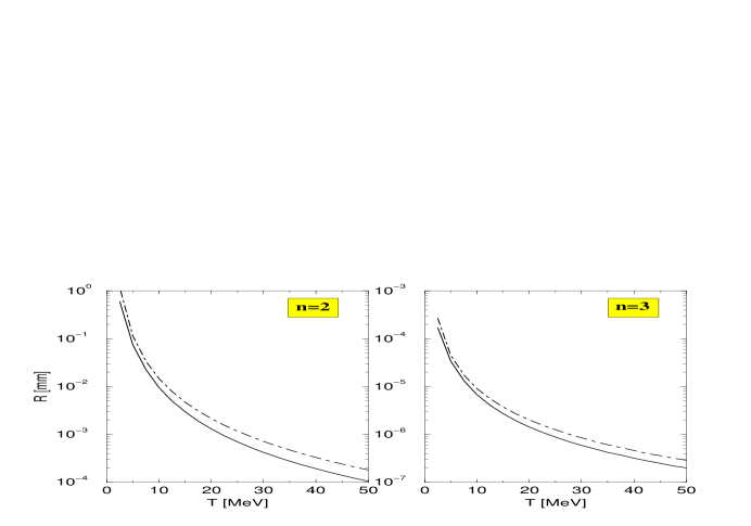
With these numerical results in hand we use the simplistic upper bound on the power per unit volume lost from SN1987a of $\dot{\cal E}_{nn}~{}=~{}10^{19}~{}{\rm ergs/g/s}$ [18] to place a bound on the radius $R$ of the extra dimensions. The resultant bounds are shown, as a function of temperature for the cases $n=2$ and $n=3$, in Fig. 2. The solid line is the result at $n_{N}=0.16~{}{\rm fm}^{-3}$, while the dot-dashed line is the result at three times nuclear matter density.

Assuming that our analysis applies to SN1987a, and using $T~{}=~{}30~{}{\rm MeV}$ and a neutron number density equal to the density of nuclear matter, our “best” bound on the compactification radius is:

$$R < 7.1\times 10^{-4}~{}{\rm mm}\ \ \ \ {\rm for}\ \ \ \ n=2,$$ (65)

$$R < 8.5\times 10^{-7}~{}{\rm mm}\ \ \ \ {\rm for}\ \ \ \ n=3.$$ (66)

These bounds are a factor of two to three weaker than those obtained by Cullen and Perelstein, who found [19]:

$$R < 3\times 10^{-4}~{}{\rm mm}\ \ \ \ {\rm for}\ \ \ \ n=2,$$ (67)

$$R < 4\times 10^{-7}~{}{\rm mm}\ \ \ \ {\rm for}\ \ \ \ n=3.$$ (68)

The source of the difference between the bounds (68) and our bound (66) will be discussed in Section V.

It is interesting to examine the energy distribution of both the radiated particles and that of the emitting nucleons, in order to determine if the soft-radiation approximation is valid. To do this, note that the kernel $K^{(n)}(\alpha,u_{r}^{\prime})$, defined in Eq. (62), may be integrated over $u_{r}^{\prime}$ or $\alpha$ in order to generate a distribution in the radiation-energy variable or the nucleon-energy variable. (Recall that $\alpha=\omega/T$ and $u_{r}^{\prime}=E_{\rm cm}^{\rm final}/(2T)$.) The results of this procedure at three different temperatures are displayed in Fig. 3, as a function of the energy of the radiation and the final-state energy of the nucleons.

FIG. 3.: Two different partial integrations of the dimensionless kernel, $K^{(n)}\left({\omega\over T},{E^{\rm final}_{\rm cm}\over 2T}\right)$, for the case $n=2$, and nuclear matter density. The solid curve corresponds to the final-state $nn$ energy distribution, while the dot-dashed curve corresponds to the radiated particle energy distribution. For $T=10~{}{\rm MeV}$ and $T=30~{}{\rm MeV}$ the curves have been multiplied by a factor of $10$ and $100$, respectively.

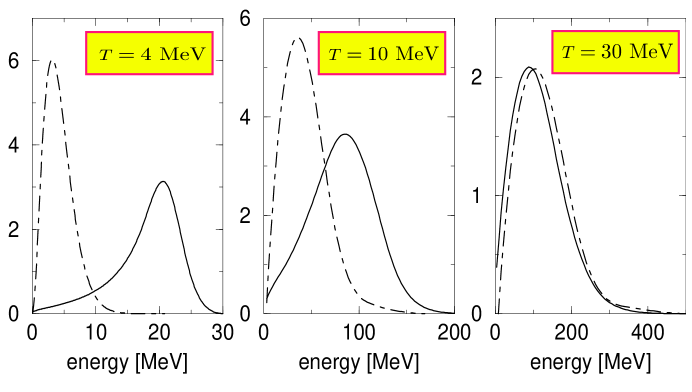
Figure 3 shows that at low temperature the typical radiated energy is much less than the typical total energy of the final-state neutrons, and so soft-radiation theorems should work very well. This is because in the degenerate limit the nucleon energy is set by $p_{F}$, while the radiation’s energy is proportional to $T$. However, as the temperature is increased, and the neutrons become non-degenerate, both energies scale with $T$. At temperatures relevant to SN1987a the radiation is seen to carry off energy comparable to that of the final-state nucleons. Note that if the neutron matter were denser then the Fermi momentum of the nucleons would be higher, and so the temperature where the peaks of the energy distributions coincide would be somewhat larger. On the other hand, as the number of extra dimensions rises the power of $\alpha$ appearing in the kernel $K^{(n)}$ increases, and so the radiation would tend to carry away even more of the $NN$ state’s energy.

The right-most panel of Fig. 3 represents the conditions used in deriving the radius bounds (66). We infer that roughly half of the initial energy of a typical $NN$ pair is radiated away to the GODs. In other words, if gravitational radiation was emitted into extra dimensions during SN1987a it may not have been soft. The parameter $\chi$, defined in Eq. (48), which we expect will control the expansion is of order 2/3 for the conditions of interest. This is a rather large value for our “small” parameter. However, the first non-vanishing correction to the emissivity is suppressed by two powers of $\chi$, which is somewhat reassuring.

IV Limiting cases and analytic formulae

While the core region of SN1987a is neither degenerate nor non-degenerate neutron matter [16], it is illuminating to consider dilastrahlung and gravistrahlung processes in these extreme cases. As we shall show in this section, in both limits analytic formulae for the emissivity in terms of one $NN$ cross section can be obtained, provided certain observations about the differential cross section are approximately true. Alternatively, effective-range theory can be used to provide a form for $\frac{d\sigma}{d\Omega}$ which can be integrated analytically. In a supernova the neutron momentum distribution lies essentially mid-way between degenerate and non-degenerate, and so these limiting cases provide bounds on the true emissivity.

A A non-degenerate neutron gas

To analyze the non-degenerate limit of neutron matter the final-state blocking factors $(1-f_{i}^{\prime})$, are set equal to unity. In other words, all of the final-state phase space is open to the scattered neutrons. In addition, the initial-state Fermi distributions are replaced by Maxwell-Boltzmann distributions. These simplifications allow the emissivity to be written in terms of integrals over the initial centre-of-mass energy distribution, the energy of the KK-dilaton or KK-graviton, and the scattering angle

$${d{\cal E}_{nn}\over dt} = \frac{8G_{N}}{3}\sqrt{\frac{T^{7}}{M}}n_{N}^{2}\,\left(RT\right)^{n}h_{n}\,\pi^{n+1\over 2}\frac{\Gamma(n+1)}{\Gamma\left(n+\frac{5}{2}\right)}\left[\frac{n^{2}+9n+23}{(2n+7)(2n+5)}\right]$$ (70)

$$\qquad\int_{0}^{\infty}d\tau\,\tau^{n+4}e^{-\tau}\int_{-1}^{1}d(\cos\theta_{\rm cm})\,\sin^{2}\theta_{\rm cm}\,{d\sigma\over d\Omega_{\rm cm}}(T\tau,\theta_{\rm cm}).$$

The variable $\tau=E_{\rm cm}^{\rm initial}/T$ is the ratio of the initial $nn$ centre-of-mass kinetic energy to the temperature ($\tau=2u_{r}$), and $n_{N}$ is the number density of neutrons. We have also used the relationship between ${\cal A}$ and the $NN$ differential cross section:

$$\frac{d\sigma}{d\Omega}=\frac{M^{2}\pi^{4}|{\cal A}|^{2}}{(2\pi)^{6}}.$$ (71)

In order to get the form (70) we had to replace the energy at which $\cal A$ is evaluated, $2T\bar{u}$, by $2Tu$, the initial-state energy. As we shall see below, this replacement makes very little difference to the final result for $\dot{\cal E}_{nn}$. In contrast, if we had employed the initial-state $NN$ energy $p^{2}/M$, instead of the average energy $\overline{p^{2}}/M$, in the pre-factor for the energy-loss rates $\frac{d\varepsilon_{X}}{d\omega}$, then the emissivity would have been larger by roughly a factor of two. However, as discussed in Sections II D and II E, the choice $\overline{p^{2}}/M$ is the one that pushes the error in the LO result to $O(\chi^{2})$. Therefore, the formula (70) is an excellent approximation to the NLO result for the emissivity in the non-degenerate limit.

We now consider two analytic forms for the $nn$ scattering cross section.

1 Nondegenerate neutron gas: energy-independent ${d\sigma\over d\Omega}$

The $nn$ differential cross section is, in fact, essentially energy-independent in the region of interest. The angular dependence is also weak, except at small angles, and the contribution of these angular regions is suppressed by the presence of $\sin^{2}\theta_{\rm cm}$. The emissivity can thus be estimated as

$${d{\cal E}_{nn}\over dt} = \frac{16G_{N}}{9}\sqrt{\frac{T^{7}}{M}}\left(RT\right)^{n}\ \pi^{{n-1\over 2}}h_{n}\ n_{N}^{2}\ \sigma^{nn}_{0}\ {\Gamma\left(n+1\right)\Gamma(n+5)\over\Gamma\left(n+\frac{5}{2}\right)}\frac{n^{2}+9n+23}{(2n+7)(2n+5)}.$$ (72)

The $nn$ total cross section can be extracted from $pp$ scattering data, provided that Coulomb effects are removed. Doing this, and evaluating $\sigma^{nn}_{0}$ at the peak of the function $\tau^{n+4}e^{-\tau}$, leads to $\sigma^{nn}_{0}=25~{}{\rm mb}$, which in turn yields bounds:

$$R < 7.0\times 10^{-4}~{}{\rm mm}\ \ \ \ {\rm for}\ \ \ \ n=2,$$ (73)

$$R < 8.3\times 10^{-7}~{}{\rm mm}\ \ \ \ {\rm for}\ \ \ \ n=3,$$ (74)

at $T=30$ MeV and $n_{N}=n_{0}$. These limits are very close to the “best” bounds (66). This indicates that, under the conditions examined here, the neutron gas is very nearly non-degenerate, and the neutrons scatter via a cross section which is almost independent of angle and energy. Note that even had the $nn$ cross section not been so flat the result (74) could still be taken as a result of naive dimensional analysis, since any “typical” $NN$ cross section will give numbers of this order of magnitude. Its success as such an estimate hinges on the fact that Eq. (72) approximates the temperature dependence of the full result very well (see Fig. 4).

2 Nondegenerate neutron gas: ${d\sigma\over d\Omega}$ From Effective-range theory

Effective-range theory (ER) describes very low-energy nucleon-nucleon scattering by a unique momentum expansion about $|\vec{p}^{\,}|=0$ [28]. Empirically, the first two terms in the expansion of $|\vec{p}^{\,}|\cot\delta$ describe the S-wave cross section well, even at energies greater than the naive breakdown scale of the expansion, which is $|\vec{p}^{\,}|=m_{\pi}/2$. The $nn$ non-relativistic differential cross section in ER is, neglecting contributions beyond the effective range,

$${{d\sigma^{nn}_{ER}}\over{d\Omega_{\rm cm}}} = \left|{1\over-{1\over a_{0}}+{1\over 2}r_{0}|\vec{p}^{\,}|^{2}\ -\ i|\vec{p}^{\,}|}\right|^{2}$$ (75)

$$\rightarrow {1\over|\vec{p}^{\,}|^{2}\left(1+{1\over 4}r_{0}^{2}\,|\vec{p}^{\,}|^{2}\right)}\ \ \ {\rm for}\ \ \ |\vec{p}^{\,}|\gg{1\over a_{0}},$$ (76)

where $a_{0}=-18.5\pm 0.4~{}{\rm fm}$ and $r_{0}=2.80\pm 0.11~{}{\rm fm}$ are the scattering length and effective range for $nn$ scattering in the ${}^{1}S_{0}$ channel [29]. As the typical momentum involved in the scattering events of interest is much larger than the inverse scattering length we take the second form for the differential cross section. Inserting this in Eq. (70) leads to a simple expression for the emissivity:

$${d{\cal E}^{\rm ER}_{nn}\over dt}=\frac{1024G_{N}}{9}\left(RT\right)^{n}\ h_{n}\pi^{1+n\over 2}\ n_{N}^{2}{\Gamma\left(n+1\right)\Gamma(n+4)\over M^{4}r_{0}^{5}\Gamma\left(n+\frac{5}{2}\right)}$$ (78)

$$\frac{n^{2}+9n+23}{(2n+7)(2n+5)}\ x^{n+{3\over 2}}e^{x}\,\Gamma\left(-(n+3),x\right),$$

with:

$$x={4\over MTr_{0}^{2}},$$ (79)

and $\Gamma\left(x,y\right)$ the incomplete Gamma function, which obeys $\Gamma\left(z,0\right)=\Gamma\left(z\right)$. The bounds obtained from the “Raffelt criterion” $\dot{\cal E}\leq 10^{19}$ ergs/g/s at $n_{N}=n_{0}$ and $T=30$ MeV are

$$R < 2.4\times 10^{-3}~{}{\rm mm}\ \ \ \ {\rm for}\ \ \ \ n=2,$$ (80)

$$R < 2.1\times 10^{-6}~{}{\rm mm}\ \ \ \ {\rm for}\ \ \ \ n=3.$$ (81)

These bounds are much weaker than the bounds (74) and (66). As expected, they give an upper bound on $R$, since the cross section (76) includes only S-waves, and other partial waves also contribute significantly to $\sigma_{0}^{nn}$ in the energy regime of interest.

B A degenerate neutron gas

Supernovae are, of course, systems far from the degenerate limit. However, the degenerate limit is of particular interest for neutron-star cooling, as stressed by Friman and Maxwell [30] and Iwamoto [31] in their respective studies of $\nu\bar{\nu}$ and axion radiation. In this section we employ some of the techniques used in Refs. [30, 31] to derive analytic formulae for this case, where $\mu/T\gg 1$.

Radiation from a degenerate neutron gas can only arise from scatterings involving neutrons near the Fermi surface in both the initial and final states. In the soft-radiation limit, the momentum of each nucleon involved in the scattering event is constrained to lie on the Fermi surface. This approximation leaves only angular and energy integrals in the calculation of the emissivity. The energy integrals are those that enter Fermi liquid theory, and are well known [32]. In particular, the energy integral that occurs in the case of $2\rightarrow 2$ scattering is

$$\int dE_{1}\,dE_{2}\,dE_{1}^{\prime}\,dE_{2}^{\prime}\ f_{1}f_{2}(1-f_{1}^{\prime})(1-f_{2}^{\prime})\delta(E_{1}+E_{2}+E_{1}^{\prime}+E_{2}^{\prime}-\omega) = {1\over 6}{\omega(\omega^{2}+4\pi^{2}T^{2})\over e^{\omega/T}-1}.$$ (82)

The $\omega$ integral can then be done analytically, leaving two angular integrations, and a result, for a degenerate neutron gas, of:

$${d{\cal E}_{nn}\over dt} = G_{N}\left(RT\right)^{n}\ h_{n}\ Y_{n}\ {T^{4}\ \Gamma\left(n+4\right)\ \pi^{{n-15\over 2}}\over 36}\int\ dt\,d\phi\,\ |\vec{p}^{\,}_{1}-\vec{p}^{\,}_{2}|^{4}\ {d\sigma\over d\Omega_{\rm cm}}\ \sin^{2}\theta_{\rm cm}$$ (83)

$$Y_{n} = \zeta(n+4)\ \ +\ 4\pi^{2}{\zeta(n+2)\over(n+2)(n+3)},$$ (84)

where $\zeta(x)$ is the Riemann Zeta function. The kinematic variables in the centre-of-mass frame are related to the integration variables $t$ and $\phi$, defined in the rest frame of the Fermi gas by

$$\cos\theta_{\rm cm} = 1-{2t^{2}\over|\vec{p}^{\,}_{1}-\vec{p}^{\,}_{2}|^{2}},$$ (85)

$$|\vec{p}^{\,}_{1}-\vec{p}^{\,}_{2}|^{2} = 2p_{F}^{2}\left[1+{t^{2}\over 4p_{F}^{2}}\ -\ \left(1-{t^{2}\over 4p_{F}^{2}}\right)\cos\phi\right],$$ (86)

where $p_{F}$ is the Fermi momentum, related to the neutron number density by $n_{N}=p_{F}^{3}/(3\pi^{2})$. Note that this method of calculation is only valid to LO in the soft expansion, since we have implicitly assumed that all nucleon momenta are on the Fermi surface.

Once again, we can now consider two approximate forms for the $nn$ scattering cross section. Firstly, evaluation of the integral appearing in Eq. (84) is straightforward if the differential cross section is independent of energy and angle. We find that

$${d{\cal E}_{nn}\over dt} = G_{N}\left(RT\right)^{n}\ h_{n}\ Y_{n}\ \sigma^{nn}_{0}\ {16\ T^{4}\ \pi^{{n-15\over 2}}\ \Gamma\left(n+4\right)\ p_{F}^{5}\over 135}.$$ (87)

On the other hand, explicit evaluation of Eq. (84) with the differential cross section of ER, Eq. (76), yields

$${d{\cal E}^{\rm ER}_{nn}\over dt} = G_{N}\left(RT\right)^{n}\ h_{n}\ Y_{n}\ {4\ T^{4}\ \pi^{n-13\over 2}\ \Gamma\left(n+4\right)\ p_{F}^{3}\over 9}\ \ D^{({\rm ER})}\left({p_{F}r_{0}\over 2}\right),$$ (88)

$$D^{({\rm ER})}\left(x\right) = {1\over x^{2}}\ -\ {\log\left[x+\sqrt{1+x^{2}}\right]\over x^{3}\sqrt{1+x^{2}}}.$$ (89)

We will not use these formulae to place bounds on $R$ from SN1987a. The nucleonic gas of SN1987a was far from degenerate, and so such bounds are not particularly meaningful.

V Discussion

In Figure 4 we present numerical results for the KK-graviton emissivity of a neutron gas, due to neutron-neutron collisions in the soft-radiation limit, at nuclear matter density. The solid curve shows numerical results obtained by using the “measured”, angle-dependent, elastic neutron-neutron differential cross section and the full Fermi distributions for the initial- and final-state nucleons. This numerical result, which is exact at the two-body level, provided the radiation is soft, is to be compared with the result given by Eq. (60) when the final-state blocking is ignored and the initial-state Fermi-Dirac distributions are replaced by Maxwell-Boltzmann distributions. This result, which is valid in the non-degenerate limit, is represented by the dotted curve. The dashed line is the analytic result (72), that is obtained by neglecting the energy and angular dependence of the $nn$ differential cross section. This function depends only on the “measured” total $nn$ cross section. Finally, the dot-dashed line is the result quoted by Cullen and Perelstein for $n=2$ in Ref. [19]:

$$\frac{d{\cal E}_{nn}}{dt}=3.7\times 10^{17}~{}\rm{ergs/g/s}\ \rho_{14}T_{\rm MeV}^{5.5}R_{\rm mm}^{2},$$ (90)

where $\rho_{14}$ is the mass density in units of $10^{14}~{}{\rm g/cm^{3}}$. Eq. (90) was derived using the one-pion-exchange approximation for the matrix element and the non-degenerate limit for the neutron gas.

FIG. 4.: Emissivity of SN1987a due to the reactions ${NN\rightarrow NN\phi}$ and ${NN\rightarrow NNh}$, calculated assuming there are two GODs of radius $R=1$ mm. The solid line is the full calculation, employing Eq. (60), while the dotted and dashed curves represent the different approximations to this discussed in the text. The dot-dashed line is the result of Cullen and Perelstein, Ref. [19].

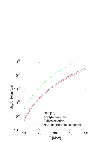
Figure 4 shows that the conditions examined here are close to the non-degenerate limit. Calculations employing this limit produce emissivities only 15% larger than the full calculation using Eq. (60). Furthermore, the approximation that the $NN$ cross section is flat in both energy and angle works exceptionally well. The effective-range theory result—which is not displayed in Fig. 4—has the wrong temperature dependence. The “full” temperature dependence—at least above $T\approx 10$ MeV—is very close to the result from a flat cross section and the non-degenerate limit: $\dot{\cal E}\,\alpha\,T^{5.5}$. The emissivity increases with temperature more slowly than this if the effective-range theory is employed because the cross section (76) drops with increasing $nn$ energy.

FIG. 5.: The seven graphs, which, together with their fermion interchange partners, were calculated to obtain the KK-graviton and KK-dilaton emissivity in previous works. The solid lines are nucleons, the dashed line is the emitted KK-graviton or KK-dilaton, and the dot-dashed line represents the pion.

The temperature dependence $\dot{\cal E}\,\alpha\,T^{5.5}$ is the same as that found in Refs. [19, 20], although Fig. 4 shows that the overall size of the emissivity (90) is significantly larger. Refs. [19, 20] both calculated KK-graviton radiation from the $NN$ system by coupling gravitons in all possible ways to the one-pion-exchange graph. The resultant diagrams are depicted in Fig. 5. The authors of both Refs. [19, 20] had graphs (a)-(d) giving zero, with graphs (e)-(g) supplying the full result. This apparently occurs because the square of the matrix element was only calculated up to order $p^{2}/M^{2}$, and graphs (a)-(d) do not contribute until $O(p^{4})$. If diagrams (e)-(g) are the full amplitude for ${NN\rightarrow NNh}$ and ${NN\rightarrow NN\phi}$ then, in the limit $m_{\pi}^{2}\ll MT$ the matrix element is constant with $\omega$ and the $NN$ system’s energy.

Our work here shows that in the soft regime, where $\omega\ll p^{2}/M$, graphs (a)-(d) will dominate over graphs (e)-(g). Consequently, if Refs. [19, 20] had examined a degenerate system, where the gravitational radiation is soft, they would have missed the dominant contribution to the emissivity, and so obtained the wrong temperature dependence. On the other hand, in the supernova case the matter is far from being degenerate, and as the discussion below Fig. 3 shows, the radiation is not especially soft. In fact, naive dimensional analysis shows that in the non-degenerate limit:

$$\frac{p^{4}}{M^{2}\omega^{2}}\sim T^{0}.$$ (91)

So, it should come as no surprise that our graphs, which represent radiation from external legs, give the same temperature dependence as graphs (e)-(g) of Fig. 5. Graphs (e)-(g) correspond to radiation from internal lines, and appear first at $O(\chi^{0})$ in our approach, but they will be accompanied there by many other diagrams. One group of additional graphs at $O(\chi^{0})$ will represent the gravitational radiation coupling to short-distance components of the $NN$ force, while another group involves the inclusion of final and initial-state interactions for the neutrons. Both of these effects should give sizeable corrections to graphs (e)-(g), and neither was included in the calculations that led to the result (90).

Thus, we would argue that the result (90) is best viewed as naive dimensional analysis of the emissivity $\dot{\cal E}_{nn}$ due to ${NN\rightarrow NNh}$. In this context, we note that either Eq. (72) or the graphs (e)-(g) of Fig. 5 can be used to estimate the emissivity for a non-degenerate gas of nucleons, and the dependence they predict on the temperature, and on the size and number of GODs, will be correct. The coefficient multiplying the overall result will differ, but it will involve “typical nuclear scales” and so it is, perhaps, not surprising that the resultant emissivities are within an order of magnitude of each other. Ultimately though, our result for $\dot{\cal E}_{nn}$ is significantly smaller than that of Refs. [19, 20], and our bounds on $R$ are correspondingly weaker.

The bounds (66) obtained in this work on the type of extra dimensions proposed in Refs. [5, 6, 7] are model-independent, and are valid under the assumptions that the radiation is soft and that two-body collisions dominate the emission. It appears that conditions in SN1987a are such that radiation from the $NN$ system is not soft enough to make the calculation we have presented here completely reliable. However, the framework described in this paper holds out the promise that corrections to our result can be systematically computed. In this way, it represents a significant advance on previous work, where uncontrolled approximations for the $NN$ dynamics were employed. Some of the higher-order corrections to the NLO result which was used to set the bounds (66) can still be expressed in terms of $NN$ system observables, e.g. derivatives of the $NN$ differential cross section with respect to angle and energy. Indeed, since the $NN$ differential cross section is essentially constant with energy and angle in the region probed by our calculation one might hope that the $O(\chi^{0})$ contribution to $\dot{\cal E}$ is fairly small. Even were higher-order corrections to halve the emissivity the bound on the radius for the $n=2$ case would still be a severe $R\ \raise 1.29167pt\hbox{$<$\kern-7.5pt\lower 4.30554pt\hbox{$\sim$}}\ 1\times 10^{-3}$ mm. This is two orders of magnitude beyond the bound attainable at any existing collider [13]. The only comparably stringent bound on the radius of toroidally-compactified, large, GODs comes from the cosmological considerations discussed by Hall and Smith in Ref. [34], who advocate $R<5.1\times 10^{-5}$ mm. However, as Hall and Smith themselves comment, this bound is subject to their ignorance of the effect that GODs have on cosmology.

In summary, for the case of two or three large, toroidally-compactified “gravity-only” dimensions one of the best bounds on modifications in the physics of gravity comes from delving into the extreme conditions present in SN1987a, and asking what effects such changes would have there. Our detailed examination of the two-nucleon dynamics which yields this bound implies that the radius of these extra dimensions must be below $7.1\times 10^{-4}$ mm for $n=2$ and below $8.5\times 10^{-7}$ mm for $n=3$.

REFERENCES

- [1] C. Caso et al., European Physical Journal, C3, 1 (1998).
- [2] I. Antoniadis, Phys. Lett. B246, 377 (1990).
- [3] E. Witten, Nucl. Phys. B471, 135 (1996).
- [4] J. Lykken, Phys. Rev. D 54, 3693 (1996).
- [5] N. Arkani-Hamed, S. Dimopoulos and G. Dvali, Phys. Lett. B 429, 263 (1998).
- [6] N. Arkani-Hamed, S. Dimopoulos and G. Dvali, Phys. Rev. D 59, 086004 (1999).
- [7] I. Antoniadis, N. Arkani-Hamed, S. Dimopoulos and G. Dvali, Phys. Lett. B 436, 257 (1998).
- [8] L. Randall and R. Sundrum, Phys. Rev. Lett. 83, 3370 (1999).
- [9] T. Han, J. D. Lykken and R.-J. Zhang, Phys. Rev. D 59, 105006 (1999).
- [10] G. F. Giudice, R. Rattazzi and J. D. Wells, Nucl. Phys. B 544, 3 (1999).
- [11] J. L. Hewett, Phys. Rev. Lett. 82, 4765 (1999).
- [12] L. Vacavant and I. Hinchliffe, hep-ex/0005033.
- [13] See, for instance, I. Antoniadis and K. Benakli, hep-ph/0004240 and hep-ph/0007226.
- [14] M. Acciarri et al. [L3 Collaboration], Phys. Lett. B470, 281 (1999); S. Mele and E. Sánchez, Phys. Rev. D 61, 117901.
- [15] G. Raffelt and D. Seckel, Phys. Rev. Lett. 60, 1793 (1988); M. Turner, ibid., 1797; H.-T. Janka, W. Keil, G. Raffelt, and D. Seckel, Phys. Rev. Lett. 76, 2621 (1996); W. Keil, H.-T. Janka, D. N. Schramm, G. Sigl, M. S. Turner, and J. Ellis, Phys. Rev. D 56, 2419 (1997).
- [16] R. P. Brinkmann and M. S. Turner, Phys. Rev. D38, 2338 (1988).
- [17] A. Burrows, R. P. Brinkmann, and M. S. Turner, Phys. Rev. D 39, 1020 (1989).
- [18] G. G. Raffelt, Stars as Laboratories for Fundamental Physics, (Chicago University Press) (1996).
- [19] S. Cullen and M. Perelstein, Phys. Rev. Lett. 83, 268 (1999).
- [20] V. Barger, T. Han, C. Kao and R. J. Zhang, Phys. Lett. B 461, 34 (1999).
- [21] F. E. Low, Phys.Rev. 110, 974 (1958).
- [22] S. L. Adler and Y. Dothan, Phys. Rev. 151, 1267 (1966).
- [23] C. Hanhart, D. R. Phillips and S. Reddy, astro-ph/0003445.
- [24] D. A. Dicus, W. W. Repko and V. L. Teplitz, hep-ph/0005099.
- [25] R. Haag, Phys. Rev. 112, 669 (1958); J. S. R. Chisholm, Nucl. Phys. 26, 469 (1961); S. Kamefuchi, L. O’Raifeartaigh and A. Salam, Nucl. Phys. 28, 529 (1961); H. D. Politzer, Nucl. Phys. B172, 349 (1980); C. Arzt, Phys. Lett. B 342, 189 (1995).
- [26] S. Weinberg, Gravitation and Cosmology: Principles and Applications of the General Theory of Relativity, John Wiley and Sons, Inc (1972). ISBN 0-471-92567-5.
- [27] Extracted from the SAID partial-wave analysis facility (http://said.phys.vt.edu/).
- [28] H. A. Bethe, Phys. Rev. 76, 38 (1949); H. A. Bethe and C. Longmire, Phys. Rev. 77, 647 (1950).
- [29] G. F. de Téramond and B. Gabioud, Phys. Rev. C 36, 691 (1987).
- [30] B. L. Friman and O. V. Maxwell, Ap. J. 232, 541 (1979).
- [31] N. Iwamoto, Phys. Rev. Lett. 53, 1198 (1984).
- [32] G. Baym and C. Pethick, Ann. Rev. Astron. Astrophys. 17, 415 (1979).
- [33] G. Raffelt and D. Seckel, Phys. Rev. D 52, 1780 (1995).
- [34] L. J. Hall and D. Smith, Phys. Rev. D60, 085008 (1999).