Spin structure of many-body systems with two-body random interactions
Abstract
We investigate the spin structure of many-fermion systems with a spin-conserving two-body random interaction. We find a strong dominance of spin-0 ground states and considerable correlations between energies and wave functions of low-lying states with different spin, but no indication of pairing. The spectral densities exhibit spin-dependent shapes and widths, and depend on the relative strengths of the spin-0 and spin-1 couplings in the two-body random matrix. The spin structure of low-lying states can largely be explained analytically.
I Introduction
Random matrix theory has been widely used to model the behavior of complex quantum systems [1, 2]. Of particular importance are two-body random matrix ensembles (TBRE), which were introduced into nuclear physics three decades ago [3, 4] and recently have received a considerable amount of renewed interest in the study of mesoscopic systems [5, 6, 7, 8, 9, 10] and nuclei [11, 12, 13, 14, 15, 16, 17, 18, 19]. This is partly due to the observation of regular structures in the low-lying states of various nuclear models with random two-body interactions. As examples we mention the observed ground state dominance of states, the occurrence of pairing (energy) gaps in random shell models [12], and the existence of vibrational and rotational bands in random interacting boson models [14]. While these observations concern the low-lying levels of many-body systems, similar regularities also have been reported in the wave function structure. These include signatures of phonon collectivity relating states of different angular momentum [12], strong pair-transfer amplitudes between ground states of nuclei with different mass numbers [17], strong electromagnetic transitions in bands of random interacting boson models [16, 19], deviations from random matrix theory in transition strength distributions for embedded Gaussian ensembles [13], and regularities in wave functions of spin systems with random interactions [18]. These observations indicate that some typical properties of interacting many-body systems are determined simply by the presence of a rotationally invariant two-body force that allows for transitions between single-particle Fock space states.
In this article we aim at an understanding of some of the reported regularities. We are particularly interested in the quantum numbers of the ground state and in correlations between energies and wave functions of low-lying states. For this purpose we consider a system of spin- fermions on orbitals, subject to a spin-conserving random two-body interaction. This system is simpler than the nuclear models studied so far, and allows us to derive analytical results. It may be seen as a model for mesoscopic systems like quantum dots.
This article is divided as follows. In the following Section we focus on the width and shape of spectral densities in sectors of definite spin for two models of spin systems with random interactions, and derive analytical results. Special emphasis is placed on understanding the spin structure of the spectrum close to the ground state. Our analysis extends and complements previous work in nuclei [14] and mesoscopic systems [10]. In Section III we investigate correlations between low-lying states, and consider pairing properties. Finally we give a summary.
II Spin Structure
A The model
We begin with a very simple model of random spin-conserving two-body interactions in a many-body system [12, 13, 14, 15, 16, 17]:
| (1) |
where and each denotes a pair of two spin fermions in a state, while and each denotes a pair of fermions in a state. The two-body states can of course be labeled by the individual orbitals occupied by the two particles. Thus, for a system with single-particle orbitals, we have pairs with total spin , enumerated as , where annihilates a single particle state, and the single-particle indices are . [Here we are enumerating two-body states with only; obviously there are equal numbers of two-body states which by rotational symmetry must couple in precisely the same way.] Similarly, there are pairs with total spin , having the form , and an additional pairs where a single site is doubly occupied: . We will assume throughout that the two kinds of states interact equally strongly among themselves and with each other; this assumption does not substantially affect any of the results to be presented in this paper. The effect of diagonal spin-spin interactions in a spin system with random wave functions has been investigated in ref. [10].
Within each two-body spin sector, then, the couplings and are assumed to be governed by a GOE random-matrix ensemble,
| (2) | |||||
| (3) |
where indicates an ensemble average. We note that the two matrices and are each taken to be real and symmetric, consistent with time reversal invariance; the model can easily be generalized to the case where an external magnetic field is present, so that the matrices must be taken from a GUE rather than a GOE ensemble, or from an intermediate ensemble [1, 2, 14]. Finally, we notice that in the model (Eq. 1), couplings in different two-body spin sectors are taken to be completely independent of one another; in Section II J we will discuss an alternative random-coupling model where this is not the case. In Section III we will see what effects on spin spectra may be obtained by adding a one-body term to the two-body random Hamiltonian. Note that the presence of a strong one-body term enhances the likelyhood of finding a spin-0 ground state, due to spin-degeneracy of the one-body spectrum.
B Preliminary results
We may now consider numerically the spectra of fermion systems interacting via the random two-body interaction of the form (Eq. 1). Due to an approximate particle-hole symmetry of this system, maximum density is obtained near half-filling, , and we may restrict ourselves to the parameter range . The preponderance of many-body ground states, which has been observed previously in shell model calculations, is seen to be an extremely strong effect in this simple random interaction model. For fermions on sites, with an exclusively spin- interaction (, ), we find for an ensemble of systems that the ground state has total spin in of the cases. For an exclusively spin- interaction (, ), the ground state is observed to have total spin for of the systems in the ensemble (a result which is statistically indistinguishable from the previous case). This is despite the fact that in this system many-body states comprise only about of the total number of states. For particles on sites, all computed ground states were observed to have total spin , independent of whether a pure or two-body coupling was used. Very similar results are obtained at least until a system size of , beyond which point the size of the many-body basis makes the diagonalization of a large ensemble of Hamiltonians prohibitively expensive. For particles on and sites, we once again observe an almost prevalence of ground states.
How may we understand these initially surprising findings within the context of a completely random interaction model? We begin by considering the shape of the many-body density of states in sectors of total many-body spin . It is known that for particles with a two-body interaction, the moments of the spectral density move away from those associated with a semicircle law, and approach those corresponding to a Gaussian shape [20, 21]. Then, the ensemble-averaged spectra , being centered at because of the symmetry of the Hamiltonian, must be described simply by their squared widths, (where denotes throughout the sum over all basis states in the sector of total spin , divided by the number of basis states in that sector). Our naive expectation (assuming that the spectrum can be described by a Gaussian shape well into its tail) is that ground state behavior should be associated with the relative widths of the different spin spectra, a preponderance of ground states arising from a large value of as compared to widths in the other sectors [10, 14]. Indeed, fixing the number of particles at , our numerical results show that for orbitals the relation is almost always observed (independent of the relative values of and ), consistent with ground state dominance. For and , however, when taking an exclusively coupling, this pattern is reversed, with the widths of the higher-spin spectra beginning to exceed those of the spectrum. This shows that the width analysis alone is not sufficient to explain numerical results for the ground state behavior. However, these findings do suggest than an interesting transition may be taking place as we approach the dilute regime, which we shall now proceed to understand analytically.
C Width analysis
The many-body basis states of the system may be classified by the total spin and the number of orbitals that are doubly occupied, . We easily see that in the dilute limit ( for fixed ), states will dominate: a typical or basis state in this limit is given for even by
| (4) | |||||
| (5) |
where the plus (minus) sign produces an () body state, the single-particle orbitals , , , , …, , are all taken to be distinct, and denotes the vacuum. However, at finite densities we must consider basis states in subsectors of different for any given value of , as these might in general have spectra of different shape and width. It is a straightforward, though somewhat tedious, counting problem to compute the ensemble-averaged squared energy width , for a typical basis state of given quantum numbers and , when acted on by the Hamiltonian (Eq. 1). For each two-particle pair or of the appropriate spin that may be annihilated, one simply has to count contributions from all pairs or that may be created in its place, while keeping track of terms that must be added up coherently. So, for example, for a pure coupling (, ), one obtains
| (6) | |||||
| (7) | |||||
| (8) | |||||
| (9) |
In Eq. 6, terms are grouped and ordered by decreasing power in the number of orbitals assuming finite density (). In particular, we notice that the leading term is invariant under particle-hole symmetry, . This symmetry is broken at because of new terms that arise in the Hamiltonian (Eq. 1) when one commutes annihilation operators and creation operators corresponding to pairs having at least one orbital in common. We notice also that the effect of double degeneracy () is initially to increase the width slightly, and then restore it to the original value when reaches its maximal value of . However, the effect of double degeneracy appears only at , which we will see below to be small compared with the level spacing near the ground state, in the many-body limit. Thus, even for a non-dilute system (), we are justified in studying the spectra of states and taking their widths as proxies for the entire spectrum of that spin, even for the purpose of determining behavior near the edge of the spectrum (where the level spacings are largest). In Section III A we will consider the possible relevance of contributions to wave function structure near the ground state. We find there that basis states with high (or low) double occupancy have almost equal overlaps with eigenstates of all energies, and have no special tendency to contribute to the low-lying part of the spectrum. Thus it appears that, to leading order, double occupancy effects are not important to understanding the spin structure of the spectrum for a pure two-body interaction.
D The four-body system
The width expression of Eq. 6 is rather unwieldy, as it consists of monomial terms, and so we begin our detailed analysis with the special case of particles; as we shall see below, all the interesting qualitative behavior of the many-body system is already present in this simple case. In the sector we have independent basis states of type , having the form
| (10) |
(where , , , and all represent different orbitals), basis states of type , and basis states of type . Similarly, in the sector we have independent basis states of type , of the form
| (11) |
and basis states of type . Finally, in the sector we only have the basis states of type . As the system becomes dilute (), type states always dominate, and the total numbers of states in the spin , , and sectors approach the ratio . [As we mentioned above, even for finite , the inclusion of states does not significantly affect the behavior of the spin spectra, leading to corrections that are small compared with the level spacing.]
What then causes the preponderance of ground states in this system? Using basis states, one obtains the following expressions for the widths (of course the part of these results is merely a special case of Eq. 6):
| (12) | |||||
| (13) |
The leading terms in the above expressions are easiest to understand. We simply need to take the number of spin- pairs in a four-body state of total spin (Eq. 10 or Eq. 11), and multiply by the number of orbital pairs to which the two particles may jump (). So, for example, in a state of total spin (Eq. 10), the and pairs are in pure combinations, while the remaining pairs are uncorrelated, i.e. of them have and have . This leads to a total of pairs each of and , explaining the two terms in the first line of Eq. 13. In a state of total spin (Eq. 11), the only difference is that the pair is now in a combination, so there are only pairs with and pairs with , leading to the and terms in the second line of Eq. 13. We see already from this very simple argument that, due to a relatively larger number of pairs in a spin- state and a relatively larger number of pairs in a spin- state, in the limit we always have if and if . The ratio of the widths in the dilute limit approaches a constant,
| (14) |
while the ratio of the many-body level spacing near the ground state, , to the width and thus to the width difference is becoming small. Because the spectral shapes approach a Gaussian form in the limit, we expect this width difference to dominate the ground-state behavior, and to see ground states for a strong coupling, and for a stronger coupling.
E The special case
The behavior for is more subtle and requires an analysis of the subleading terms in Eq. 13. To compute these we need to count more carefully the number of places or to which the two interacting particles may jump, given that two of the orbitals remain occupied by the two ‘bystanders’ during the interaction. In the case of a pair, we also need to treat correctly the interference between terms. The end result is that overall, after adding together and couplings, the width is suppressed at compared with the width, as a simple physical argument shows. In Eq. 10, the pair (or any one of the other analogous pairs) may interact either in a or combination, with the final state leaving doubled up with and with ending up on any of the remaining sites. For an initial state of the form Eq. 11, this process is not allowed (since the pair start out in a spin-symmetric combination and cannot end up occupying the same orbital), so is reduced at the level. Thus, in the large- limit for , we obtain
| (15) |
By itself, however, this width difference should not be sufficient to determine the ground state behavior. That is because for a Gaussian spectral density with states the location of the ground state scales as , while the level spacing near the ground state goes as . So the ratio of the expected difference (gap) between the lowest and states to the level spacing scales as
| (16) |
and thus in a model of random uncorrelated fluctuations under the two Gaussian spectral envelopes and , we would expect no preference for either or ground states (i.e. the ratio of to ground states should approach the ratio valid for the total density of states). We note, however, that in our numerical simulations, the ground state always comes out to have spin , even for the highest values of () that we can achieve, where the width difference is very small. Indeed, as we saw above in Section II D, ground states can dominate even when the width difference changes sign, as happens for a pure spin- two-body coupling (). A major reason for this we believe to be strong deviations from the Gaussian shape of a four-particle spectrum (though correlations between and may also be relevant; we will discuss these correlations in more detail in Section III B).
F Spectral shape effects
We recall that the approach of an body spectrum to a Gaussian shape given only two-body interactions depends crucially on the assumption that repeated applications of the Hamiltonian act on different pairs of particles and therefore may be taken to commute with each other. So, for example,
| (17) | |||||
| (18) | |||||
| (19) | |||||
| (20) |
where , , , and label two-body states (either or ), as in Eq. 1, and are summed over. Notice that the third term contributes in general only if the two transitions involve distinct pairs of interacting particles. Otherwise (e.g., for a generic sparse matrix with no two-body interaction structure), we would obtain , the relation appropriate to a semicircular spectral shape rather than to a Gaussian [20, 21, 22]. So the extent to which the spectrum deviates from a Gaussian shape towards a semicircle may be estimated by considering the probability that successive two-body interactions do not involve distinct pairs of particles.
Consider for example a pure two-body coupling. In an four-body state (Eq. 10), there are a total of three pairs, as we have already seen above. After two of the particles interact in a two-body combination, the remaining two particles are guaranteed to be also in a state. So there is a probability that the next interaction will involve the two particles that have not yet interacted, and thus . On the other hand, if the total many-body state is either (Eq. 11) or , similar counting arguments lead to the conclusion that there is only a probability that the second interacting pair will be disjoint from the first; thus . This behavior for the spectral shapes has been numerically confirmed (e.g., for orbitals, , , and , for total many-body spin , , and , respectively), and is similar for the two-body interaction. So in particular for the case of equal couplings, although the widths of the and spectra approach each other in the limit (Eq. 15), the fourth moments remain in a finite ratio in this limit and lead to having a substantially longer tail than . Therefore, despite the almost equal widths, ground states in a system will be predominantly , even in the dilute limit.
G The general many-body problem
The above analysis of the particle system generalizes easily to the real -body problem that we are interested in. We begin, as before, by addressing the behavior of the spectral widths in the and spin sectors. Typical basis states in these two sectors were already given above in Eq. 5. Now consider a pure coupling. From Eq. 6 we get
| (21) |
in the dilute limit. This can be understood as follows. The only difference scaling as in the spectral width is that the pair in Eq. 5 is in a combination for a many body-state of total spin , but not if the many-body state has total spin . Thus, the state has one more pair that can be acted on by the Hamiltonian, out of a total of pairs with . Similarly, for a pure coupling we have one extra pair that can be acted on in an many-body state (out of a total of pairs with ), so finally
| (22) |
If we keep the number of particles fixed and take the system size , then the many-body level spacing of course goes to zero, while the width ratio remains finite for . Once again we see, this time for general values of , that assuming the spectral structure is dominated by the spectral width, we expect () ground states if (), in the dilute limit.
However, we saw in our discussion above of the special case that spectral cumulants beyond need also to be included in a full analysis. The ratio always favors a longer tail for , so we only need to consider the case of a coupling, where the width effect and the spectral shape effect are competing with one another. Referring back to Eq. 5, we note that if particles on orbitals and interact via a two-body interaction, then the two particles which remain on sites and are also in a state and can subsequently interact if and only if the total system is in an state (so that the four particles , , , are in an state). Because the , pair is distinct from the , pair by construction, this causes it to be more likely that the next pair of interacting particles will be distinct from , if , and contributes towards an enhancement of the shape ratio as compared with . However, in a many-body system this effect is suppressed by (because there are ways to choose two pairs, and only of them are involved in this effect). So for the difference in widths between and (Eq. 22) is expected to exceed the difference in spectral shapes, leading to a dominance of states near the edge of the spectrum, in the dilute many-body limit (which we define as first, followed by ).
For , on the other hand, both the difference in widths and difference in spectral shapes favors an ground state, and this behavior is expected to persist into the dilute many-body limit. For , the relative width difference vanishes (Eq. 22) in this limit, but the difference in spectral shapes now takes over, again leading to dominance near the edge of the spectrum.
H Transition at finite densities
We have seen that for finite (large enough) number of particles , ground state dominance is expected in the dilute limit, as long as the spin-zero two-body coupling is at least as large as the spin-one coupling, . In the contrary case, the situation is reversed, with higher-spin states dominating behavior near the edge of the spectrum. What happens, though, if the system is not very dilute? For a finite number of single-particle orbitals , we must take into account the subleading behavior in of the spectral widths. An argument very similar to the one leading to Eq. 15, but generalized to large and to an arbitrary ratio of couplings shows that the effect discussed there always favors the width, at , independent of which coupling is stronger. So for nothing particularly interesting happens at finite densities; the preference for states near the edge is only enhanced by finite density effects. This preference, however, becomes small (compared to the level spacing) in the many-body limit.
On the other hand, for a stronger spin- coupling (), we expect the effect favoring ground states and the effect favoring ground states to balance each other, leading to a transition in the width ratio at finite densities. In fact a closer analysis of the body system (Eq. 13), setting equal the terms proportional to in the two expressions, shows that for a pure coupling we have a transition just below , with a larger width for and larger widths for . This is consistent with our numerical observations above. For comparable coupling strengths, the transition of course will take place at lower densities; so, for example for , the transition in the width ratio occurs near . Although we are unable to observe this transition numerically for larger numbers of particles, the analytical arguments suggest that one should take place in general at densities for a small coupling difference and at an finite density for a pure interaction.
I Numerical results
In Table I we show some results of a numerical calculation for particles distributed over orbitals, with a pure two-body coupling (, ). The first row of the Table shows the ratio of widths in sectors of total many-body spin and . We see that holds at low (high density), while in the dilute regime () the relation is reversed. The crossover occurs near for , in good agreement with our analytical expectations (see Section II H). The same qualitative behavior is predicted and observed for the higher spin sectors; we see from the second row of the Table that the crossover between and dominance occurs at .
We proceed to compare the energies of the lowest-lying states in the different spin sectors, and find a trend towards lower-lying states of higher spin as increases, entirely consistent with the results for the spectral widths. However, by comparing rows 1 and 3 (or 2 and 4) of the Table, we see that for any given system size , low-lying states with small total spin are preferred more than would be expected based simply on the width ratio. Thus, for , where the spin- and spin- widths are nearly equal, the ground state of the system is still nearly always , and on average the ground state is observed to have energy lower than that of the lowest state. This is due largely to the spectral shape effects discussed above in Section II F, which favor ground states of lower total spin given equal spectral widths in the different spin sectors.
When comparing and sectors in particular, we recall from Section II F that the ratio is significanlty larger for , for any value of . For (see Section II G), spectral shape effects are reduced, but unfortunately we are unable to probe the dilute regime numerically for . Instead we stay at particles and compare the and sectors, which as we saw previously have nearly equal values of the ratio . Indeed, by the mean values of the lowest-lying and states become almost equal, and already by the lowest-lying state appears before the lowest-lying state in a significant fraction of systems in the ensemble. The last row of the Table supports the analytical arguments presented above for a transition between lower-spin and higher-spin ground states as a function of the particle density.
J An alternative model
As we have mentioned previously, the model (Eq. 1) assumes that there is no correlation between two-body interactions in and two-body states. We may instead consider an alternative model, motivated by Ref. [20] and much subsequent work, in which the interaction Hamiltonian is separated into a spin-independent and a spin-dependent part:
| (23) | |||||
| (24) |
where the indices and label individual orbitals, and are the components of spin for each of the four fermions, and total spin conservation has been enforced. The matrix elements and are taken to be real Gaussian random and independent variables, with the constraints
| (25) |
(and similarly for the ) imposed by the reality of wave functions and the symmetry of the two-body interaction. The constants and determine, of course, the relative strengths of the spin-independent and spin-coupled interactions.
The behavior near the ground state for the model of Eq. 24 can be understood in terms very similar to those we used for analyzing the original model of Eq. 1. We assume initially that spin-spin interactions cannot be neglected, i.e. . We first note that the spin-spin interaction is three times stronger when particles and are in a two-body state as compared with a two-body state. Now we have seen above that an particle many-body state has more pairs than an many body state: this leads to a wider envelope and ground state dominance, just as for the situation considered in the previous model. Thus, a spin-spin interaction (of either sign) is seen immediately to lead to ground state dominance ( dominance in the many-orbital limit). At finite densities, , we must once again include corrections to the width difference, of order , as in Eq. 15 and in Section II H above. We find, however, that the subleading correction, associated with the impossibility of doubling up two particles in a two-body state, always favors the many-body state. This is a model-independent property, resulting simply from the counting of two-body vs. pairs in a many-body state. Therefore the and effects contribute with the same sign, and even at finite density we expect an excess of ground states. Finally, for small systems, shape effects (discussed above in Section II F) also contribute, again favoring the ground state.
We may also consider the scenario of a spin-free interaction (), which because of the equal strength with which it couples and pairs may be compared with the special case discussed above for the model of Eq. 1. As in that case, the width difference is now expected to vanish in the dilute limit; furthermore as before the width difference eventually becomes small compared with the level spacing in the system. However, at moderate values of the particle number , spectral shape effects are expected to be very important, leading to ground state excess at arbitrarily large values of .
III Correlations and Pairing
In realistic many-body systems there are strong correlations between ground states of different quantum numbers, and the pairing correlation is of particular importance. This correlation has also been observed in various studies of nuclear models with random two-body interactions [12, 14, 17]. In this Section we investigate correlations between energies and wave functions of low lying states with different quantum numbers.
A Pairing
Pairing is a well known phenomenon in many-body fermion systems. Its spectral signature is an energy gap that separates the ground state from the excited states. In the presence of pairing, the ground state is a condensate of pairs of fermions whose quantum numbers are related to each other by time reversal symmetry. In the case of the spin systems considered in this work, pairing refers to a ground state of the form , where is a quasi-particle operator that is related to the single-particle operators by a unitary transformation, as .
Let us first consider pairing in the single-particle basis generated by the . The results on wave function structure in random spin systems reported in Ref. [18] show that states at high spectral densities have a number of principal components that agrees with standard random matrix theory, while low-lying states have a considerably smaller number of principal components (thus indicating a simpler structure and some degree of regularity [23, 24]). However, the structure even of the low-lying states was found to be much more complex than a simple Slater determinant. Based on that previous analysis, and on the analytical results obtained above in Eq. 6 showing very weak dependence of spectral width on double occupancy number, we do not expect to find pairing here in the single-particle basis. To compare these arguments with numerical data we measure the number of doubly occupied single-particle orbitals in a given eigenstate with energy and total spin by computing (compare the related quantity for basis states in Section II C). For an ensemble of random Hamiltonians with spin- fermions on sites, and , shows fluctuations around , , and does not exhibit any significant energy dependence. Thus, no pairing is present in the single-particle basis . The numerical results agree well with the analytical expressions , , and .
Pairing in a general quasi-particle basis can most conveniently be investigated by examining its spectral signature. The existence of a pairing gap is closely related to the approximate degeneracy of the first excited spin-0 level with the lowest-energy spin-one state . Within the two different models considered in this work, we do not observe any degeneracy between and , and find the ratio of splitting to gap as
| (26) |
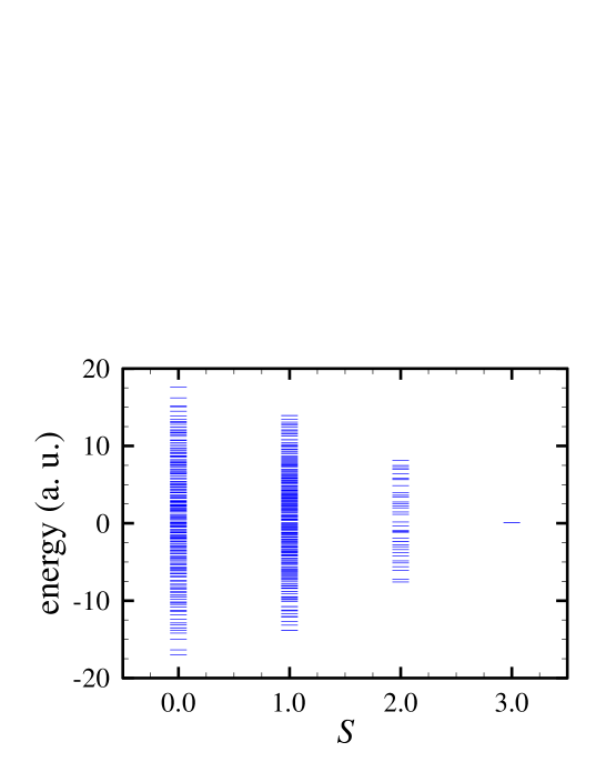
for an ensemble of Hamiltonians with , , and . Similar results hold for other parameter values, and we never see , which would be indicative of a pairing structure. Thus, the dominance of spin-0 ground states cannot be caused by pairing correlations within our model. Note that this result differs from the observations made for the nuclear shell model with random interactions [12, 17, 14]. As an illustration we show in Fig. 1 the spin dependent spectra for a system of six fermions on six single-particle orbitals. The random two-body interactions only couple pairs of spin , i.e. we set . The ground state and the low energy states have spin . The absence of low-lying spin-degenerate states clearly indicates the absence of pairing correlations.
To study further the subject of pairing, we add a one-body part of the form
| (27) |
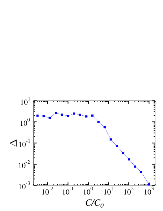
to the Hamiltonian (Eq. 1). Fig. 2 shows the pairing observable as a function of for and . For we find , indicating strong pairing. In this regime the two-body interaction is a small perturbation, and we obtain pairing in the basis of single particle states. Note that this behavior is not caused by the harmonic form of our one-body potential but rather is determined by the applicability of a single-particle picture. For decreasing values of one leaves this perturbative regime, and the increase of shows that pairing is suppressed. Note that at sufficiently small values of . This indicates that there are several spin-0 levels below the spin-1 ground state, as in Fig. 1 above. This finding is consistent with the results of Section II and hints at the dominance of spin-0 low-lying states. As a check we also replaced the spin-1 ground state energy by the highest spin-1 energy (which should not be at all correlated with the spin-0 ground state energy), while correcting for a nonzero mean of the total spectral density, i.e. replacing , and recomputed . For the system with a pure two-body force we found no difference when compared to the previous results, confirming that the value of at is consistent with random spectral fluctuations.
B Level and energy correlations
The absence of pairing in the presence of a strong two-body force is peculiar to our model and is not shared by nuclear shell models with random interactions. It is therefore interesting to look for different correlations between low lying states of spin-0 and spin-1. Such correlations have been observed previously in Refs. [12, 17]. We therefore look at the generalized collectivity defined as
| (28) |
where and
| (29) |
is a spin-flip operator that transforms a pair of spin zero into a pair of spin one. Following Refs. [12, 17] we choose the coefficients as
| (30) |
This is more convenient than searching for those coefficients that maximize . To be definite, we take the ground states of spin zero and spin one, i.e. and , and compare with the corresponding value that is obtained by substituting . The states corresponding to the highest and lowest energies in a sector of definite spin are assumed to be uncorrelated. The results are presented in Table II for and different values of , once again setting . Obviously, there is a strong correlation between the ground states of different spin. It is instructive to let run through the lowest lying spin- states while keeping fixed. Figure 3 shows that the correlation is strongest for the ground states and decreases for the higher lying states. This finding is consistent with the recent observation [18] that low-lying states are weakly localized in Fock space, while high-lying states are delocalized and agree with random matrix predictions.
It is also interesting to consider energy correlations between ground states of spin zero and spin one. The appropriate correlator is
| (31) |
where and denotes an ensemble average. We find for particles on sites (with ), indicating a strong correlation. The observable , is however, somewhat misleading, since a significant part of the fluctuations from one realization of the ensemble to another arises simply from the fluctuation of the centroid and width of the overall spectral envelope, and . The centroid and width for a given system are almost identical in sectors of different total many-body spin. To understand fluctuations under the spectral envelopes, we should therefore remove this trivial effect by considering the correlation of and , where
| (32) |
We then obtain for the same set of parameters. The value of increases as one goes to larger systems; e.g. for particles, increases monotonically from to as goes from to . These observations are consistent with the existence of correlations between the wave functions of the corresponding states.
Note that the observation of strong correlations between low-lying states of spin-0 and spin-1 is in qualitative agreement with results in shell models and interacting boson models. However, in contrast with the findings in these nuclear models, we do not find any indications of a pairing correlation in the spin systems considered in this work. One can only speculate that this is due to the additional isospin degrees of freedom and the more sophisticated angular momentum coupling scheme used in the nuclear models.
IV Summary
We have investigated the spin structure of low lying states in fermion systems with random two-body interactions. Numerical calculations show that the ground state has spin zero with almost 100% probability. For a dilute system we derive analytical expressions for the shapes and widths of the spectral densities at different spin. These explain our numerical results. For systems with a spin-1 coupling that is stronger than the spin-0 two-body coupling we predict a transition from spin-0 ground states to ground states of higher spin. While it is difficult to access this regime numerically, we do observe one of its precursors – namely a spin-2 ground state that is lower in energy than the spin-1 ground state.
Furthermore, we have shown that there are strong correlations between wave functions and energies of low-lying states of different spin quantum number. The wave function correlations are manifest in expectation values of spin transition operators and indicate some degree of collective behavior. The existence of energy correlations confirm the picture about the dominance of spin-0 ground states. These correlations decrease as one moves away from the ground state region. In the absence of a one-body force we find no indication for any pairing correlation between low lying states, and our model differs herein from the nuclear models with random interactions. Pairing correlations are only observed after a sufficiently strong one-body potential is added to the random Hamiltonian.
Acknowledgments
We acknowledge useful discussions with R. Bijker, A. Frank, and T. H. Seligman, and we particularly thank G. F. Bertsch for providing the original motivation and making many helpful suggestions. This work was partially supported by Department of Energy.
REFERENCES
- [1] T. A. Brody, J. Flores, J. B. French, P. A. Mello, A. Pandey, and S. S. M. Wong, Rev. Mod. Phys. 53, 385 (1981).
- [2] T. Guhr, A. Müller-Groeling, and H. A. Weidenmüller, Phys. Rep. 299, 189 (1998).
- [3] J. B. French and S. S. M. Wong, Phys. Lett. B 33, 449 (1970).
- [4] O. Bohigas and J. Flores, Phys. Lett. B 34, 261 (1971).
- [5] Ph. Jacquod and D. L. Shepelyansky, Phys. Rev. Lett. 79, 1837 (1997).
- [6] P. G. Silvestrov, Phys. Rev. E 58, 5629 (1998).
- [7] C. Mejia-Monasterio, J. Richert, T. Rupp, and H. A. Weidenmüller, Phys. Rev. Lett. 81, 5189 (1998).
- [8] V. V. Flambaum and F. M. Izrailev, Phys. Rev. E 61, 2539 (2000).
- [9] Y. Alhassid, Ph. Jacquod, and A. Wobst, Phys. Rev. B 61, R13357 (2000).
- [10] Ph. Jacquod and A. D. Stone, Phys. Rev. Lett. 84, 3938 (2000).
- [11] V. Zelevinsky, Ann. Rev. Nucl. Part. Sci. 46, 237 (1996).
- [12] C. W. Johnson, G. F. Bertsch, and D. J. Dean, Phys. Rev. Lett. 80, 2749 (1998).
- [13] V. K. B. Kota and R. Sahu, Phys. Lett. B 429, 1 (1998).
- [14] R. Bijker, A. Frank, and S. Pittel, Phys. Rev. C 60, 021302 (1999).
- [15] V. K. B. Kota, R. Sahu, K. Kar, J. M. G. Gómez, and J. Retamosa, Phys. Rev. C 60, 051306 (1999).
- [16] R. Bijker and A. Frank, Phys. Rev. Lett. 84, 420 (2000).
- [17] C. W. Johnson, G. F. Bertsch, D. J. Dean, and I. Talmi, Phys. Rev. C 61, 014311 (2000).
- [18] L. Kaplan and T. Papenbrock, Phys. Rev. Lett. 84, 4553 (2000).
- [19] R. Bijker and A. Frank, Phys. Rev. C 62, 014303 (2000).
- [20] A. Gervots, Nucl. Phys. A 184, 507 (1972).
- [21] K. K. Mon and J. B. French, Ann. Phys. 95, 90 (1975).
- [22] A. P. Zuker, arXiv:nucl-th/9910002
- [23] Y. V. Fyodorov and A. D. Mirlin, Phys. Rev. B 51, 13403 (1995).
- [24] Y. V. Fyodorov and A. D. Mirlin, Phys. Rev. B 56, 13393 (1997).
| 5 | 6 | 7 | 8 | 9 | 10 | 11 | 12 | |
| 1.20 | 1.13 | 1.09 | 1.06 | 1.03 | 1.01 | 1.00 | 0.99 | |
| 1.21 | 1.12 | 1.07 | 1.03 | 0.99 | 0.97 | 0.95 | 0.94 | |
| 1.40 | 1.27 | 1.21 | 1.17 | 1.14 | 1.11 | 1.12 | 1.09 | |
| 1.89 | 1.40 | 1.21 | 1.14 | 1.07 | 1.03 | 1.02 | 1.01 | |
| 0% | 0% | 0% | 0% | 0% | 0% | 0% | ||
| 0% | 0% | 0% | 10% | 20% | 20% | 70% |
| 4 | 5 | 6 | 7 | 8 | 9 | |
|---|---|---|---|---|---|---|
| 0.45 | 0.37 | 0.33 | 0.29 | 0.24 | 0.26 | |
| 0.11 | 0.05 | 0.03 | 0.02 | 0.01 | 0.01 |