Photons from Ultra-Relativistic Heavy Ion Collisions
Thesis submitted in partial fulfilment of
the requirement for the Degree of
Doctor of Philosophy (Science)
of the
University of Calcutta
Saurabh Sarkar
Variable Energy Cyclotron Centre
Department of Atomic Energy
1/AF Bidhannagar, Calcutta-700 064
March 2000
Acknowledgements
It gives me great pleasure to thank Prof. Bikash Sinha for being a constant source of inspiration ever since I took up theoretical physics as my career. I have been very fortunate to have enjoyed his guidance as the Director of my Institute, VECC, my thesis supervisor, and most importantly, as a close and warm-hearted colleague; an experience which I will cherish throughout my life.
I express my sincere gratitude to Prof. Binayak Dutta-Roy for being a great teacher and an enthusiastic collaborator. Discussions with him has helped me to clarify numerous basic concepts of physics, particularly Quantum Field Theory.
I am very grateful to Dr. Dinesh Kumar Srivastava, with whom I have been associated from the beginning, for always being very helpful to me.
It is a pleasure to thank Dr. Jan-e Alam and Dr. Pradip Roy who have contributed immensely to the work reported in this thesis. I sincerely look forward to their association in future years. I am immensely grateful to Prof. T. Hatsuda for many helpful discussions and guidance.
I also take this opportunity to thank Prof. Sibaji Raha, Dr. Abhijit Bhattacharyya, Dr. Subhasis Chattopadhyay and Ms. Dipali Pal with whom I have enjoyed working over the years. Special thanks are due for Dr. Tapan Nayak for clarifying various aspects regarding experiments. I also express my gratitude to Dr. Jadu Nath De, Dr. Y. P. Viyogi and Dr. Santanu Pal for their support and advice.
The encouragement, patience and tenderness from my wife Jui and little daughter Sebanti have been the essential ingredients to go through this task of writing my thesis.
Saurabh Sarkar
VECC, Calcutta
List of Publications
-
1.
Rapidity Distribution of Photons Emitted from a Hadronizing Quark Gluon Plasma,
S. Sarkar, D. K. Srivastava, and B. Sinha. Phys. Rev. C51 (1995) 318. -
2.
Effects of a Sharp Boundary on Thermal Photons from Quark Gluon Plasma,
S. Sarkar, P. K. Roy, D. K. Srivastava, and B. Sinha.
J. Phys. G22 (1996) 951. -
3.
A Scheme to Identify Transverse Collective Flow in Relativistic Heavy Ion Collisions at CERN SPS,
D. K. Srivastava, S. Sarkar, P. K. Roy, D. Pal, and B. Sinha, Phys. Lett. B379 (1996) 54. -
4.
Soft Photons from Relativistic Heavy Ion collisions,
P. K. Roy, D. Pal, S. Sarkar, D. K. Srivastava, and B. Sinha, Phys. Rev. C53 (1996) 2364. -
5.
Dissipative Effects in Photon Diagnostics of Quark Gluon Plasma,
S. Sarkar, P. K. Roy, J. Alam, S. Raha, and B. Sinha, J. Phys. G23 (1997) 467. -
6.
Large Mass Diphotons from Relativistic Heavy Ion Collisions,
S. Sarkar, D. K. Srivastava, B. Sinha, P. K. Roy, S. Chattopadhyay and D. Pal, Phys. Lett. B402 (1997) 13. -
7.
Soft Electromagnetic Radiations from Relativistic Heavy Ion Collisions,
D. Pal, P. K. Roy, S. Sarkar, D. K. Srivastava, and B. Sinha, Phys. Rev. C55 (1997) 1467. -
8.
Thermal Masses and Equilibration Rates in Quark Gluon Plasma,
J. Alam, P. K. Roy, S. Sarkar, S. Raha, and B. Sinha, Int. J. Mod. Phys. A12 (1997) 5151. -
9.
Quark Gluon Plasma Diagnostics in a Successive Equilibrium Scenario,
P. K. Roy, J. Alam, S. Sarkar, B. Sinha, and S. Raha, Nucl. Phys. A624 (1997) 687. -
10.
Photons from Hadronic Matter at Finite Temperature,
S. Sarkar, J. Alam, P. Roy, A. K. Dutt-Majumder, B. Dutta-Roy, and B. Sinha, Nucl. Phys. A634 (1998) 206. -
11.
Unstable Particles in Matter at a Finite Temperature: the Rho and Omega Mesons,
J. Alam, S. Sarkar, P. Roy, B. Dutta-Roy, and B. Sinha, Phys. Rev. C59 (1999) 905. -
12.
Omega Meson as a Chronometer and Thermometer in Hot and Dense Hadronic Matter,
P. Roy, S. Sarkar, J. Alam, B. Dutta-Roy, and B. Sinha, Phys. Rev. C59 (1999) 2778. -
13.
Electromagnetic Radiations from Hot and Dense Hadronic Matter,
P. Roy, S. Sarkar, J. Alam, and B. Sinha, Nucl. Phys. A653 (1999) 277. -
14.
Photons from Pb+Pb and S+Au Collisions at Ultrarelativistic Energies,
S. Sarkar, P. Roy, J. Alam, and B. Sinha, Phys. Rev. C60 (1999) 054907. -
15.
Cosmological QCD Phase Transition and Dark Matter,
A. Bhattacharyya, J. Alam, S. Sarkar, P. Roy, B. Sinha, S. Raha, and P. Bhattacharjee, Nucl. Phys. A661 (1999) 629c.
Abstract
It is believed that a novel state of matter - Quark Gluon Plasma (QGP) will be transiently produced if normal hadronic matter is subjected to sufficiently high temperature and/or density. We have investigated the possibility of QGP formation in the ultra-relativistic collisions of heavy ions through the electromagnetic probes - photons and dileptons. The formulation of the real and virtual photon production rate from strongly interacting matter is studied in the framework of Thermal Field Theory. Since signals from the QGP will pick up large backgrounds from hadronic matter we have performed a detailed study of the changes in the hadronic properties induced by temperature within the ambit of the Quantum Hadrodynamic model, gauged linear and non-linear sigma models, hidden local symmetry approach and QCD sum rule approach. The possibility of observing the direct thermal photons and lepton pairs from quark gluon plasma has been contrasted with that from hot hadronic matter with and without medium effects for various mass variation scenarios. The effects of medium induced modifications have also been incorporated in the evolution dynamics through the equation of state. We find that the in-medium effects on the hadronic properties in the framework of the Quantum Hadrodynamic model, Brown-Rho scaling and Nambu scaling scenarios are conspicuously visible through the low invariant mass distribution of dileptons and transverse momentum spectra of photons. We have compared our evaluation of the photon and dilepton spectra with experimental data obtained by the WA80, WA98 and CERES Collaborations in the heavy ion experiments performed at the CERN SPS. Predictions of electromagnetic spectra for RHIC energies have also been made.
List of Symbols
| transverse projection tensor | |
| longitudinal projection tensor | |
| free vacuum propagator for spin 1 particles | |
| matrix propagator for spin 1 particles at finite temperature | |
| retarded propagator for spin 1 particles | |
| field tensor for electromagnetic field | |
| Bose distribution | |
| Fermi distribution | |
| the metric tensor (1,-1,-1,-1) | |
| time-ordered free thermal propagator for nucleons | |
| Hartree nucleon propagator; vacuum part | |
| Hartree nucleon propagator; medium part | |
| hadronic (leptonic) electromagnetic current | |
| leptonic tensor | |
| invariant amplitude | |
| Borel mass | |
| nucleon mass | |
| mass of vector meson | |
| the invariant mass | |
| transverse momentum | |
| thermodynamic pressure | |
| entropy density | |
| vector mesons | |
| three volume | |
| electromagnetic current correlation function | |
| partition function at temperature | |
| electromagnetic coupling constant, | |
| strong coupling constant, | |
| totally antisymmetric tensor, with | |
| thermodynamic energy density | |
| width of the vector meson | |
| four-volume | |
| proper self energy for spin 1 particles | |
| spectral function for spin 1 particles | |
| non-abelian field tensor for the rho meson |
Chapter 1 Introduction
As per contemporary wisdom, hadrons i.e. baryons and mesons are made up of quarks which interact by the exchange of gluons. This interaction is governed by a non-abelian gauge theory called Quantum Chromodynamics (QCD). Gluons, the gauge particles of QCD unlike photons of Quantum Electrodynamics, carry colour charge and are self interacting. This endows the QCD interaction with remarkable properties as a function of the relative separation, or equivalently, the exchanged momenta. At short distances, or large momenta , the effective coupling constant decreases logarithmically. This means that the quarks and gluons appear to be weakly coupled at very short distances, a behaviour referred to as asymptotic freedom [1, 2]. At large separations, the effective coupling, it is believed, progressively turns stronger resulting in the phenomena called quark confinement [3, 4, 5] which describe the observation that quarks do not occur isolated in nature, but only in colour singlet hadronic bound states as mesons (quark-antiquark bound states) and baryons (three quark bound states). In this case one also has chiral symmetry breaking [6] which expresses the fact that the quarks confined in hadrons do not appear as nearly massless constituents but are endowed with a dynamically generated mass of several hundred MeV. In nature there exist six quark flavours of three colours in addition to eight bi-coloured gluons.
The QCD renormalization group calculation predicts that as the temperature and/or density of strongly interacting hadronic matter is increased, the interactions among quanta occur effectively at very short distances and is thus governed by weak coupling due to asymptotic freedom, while the long range interactions become dynamically screened due to Debye screening of colour charge [7, 8, 9]. The interaction thus decreases both at small distances as well as for distances large in comparison to typical hadronic dimensions. As a consequence, nuclear matter at very high temperature/density exhibits neither confinement nor chiral symmetry breaking. This new phase of QCD where the bulk properties of strongly interacting matter are governed by the fundamental degrees of freedom - the quarks and gluons, in a finite volume is known as the state of quark gluon plasma (QGP).
There are sufficient reasons to expect that the transition between the low and the high temperature manifestations of QCD is not smooth but exhibits a discontinuity, indicating the occurrence of a phase transition at some intermediate value of temperature [10, 11]. In this context one refers to the possibility of two different kinds of phase transitions, namely, the chiral symmetry restoring transition and the deconfinement transition. Now, it is necessary to realize that though QCD is firmly established as the theory of strong interactions, the long range behaviour of QCD is not well understood. This is because, at larger separations the strong coupling becomes large and invalidates perturbative approaches. As a result the study of long range phenomena such as phase transitions and hadronic properties and interactions using QCD is highly inhibited. One of the attempts to study such phenomena non-perturbatively on a discrete space-time lattice is the lattice gauge theory [12].
At low energies, the QCD vacuum is characterized by non-vanishing expectation values of certain composite operators, called vacuum condensates e.g. which describe the non-perturbative physical properties of the QCD vacuum. They also act as the order parameter for the chiral phase transition. QCD calculations on the lattice suggest a first order (discontinuous) chiral transition for two massless quark flavours and a second order (smooth) transition for three flavours. The chiral phase transition is indicated by a strong drop in the value of the condensate at the transition temperature, believed to have values between 130-160 MeV. Lattice calculations also indicate that there is a sharp change in the energy and entropy densities at [13]. This can be interpreted as an increase in the number of degrees of freedom, corresponding to a deconfinement transition. Thus restoration of chiral symmetry and deconfinement seem to occur concomitantly.
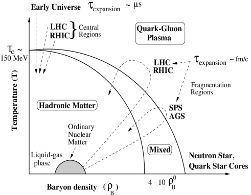
The quark-hadron phase transition is also expected to occur at high baryon density even at zero temperature. There is however a large uncertainty in the critical baryon density of transition. Model calculations predict critical densities to lie anywhere between 4 to 10 times normal nuclear matter density. One expects a smooth connection between the high temperature and high baryon density phase transitions, giving rise to a continuous phase boundary . Fig. (1.1) shows a typical phase diagram of strongly interacting matter. For , the effective description is in terms of hadronic degrees of freedom, whereas for the degrees of freedom carry the quantum numbers of quarks and gluons. However, recently very interesting theoretical developments regarding the QCD phase diagram has taken place. At high densities, quarks may form Cooper pairs and a new colour superconducting phase may exist. The phase diagram may have a critical or tricritical point somewhere along the phase transition line [14, 15, 16].
According to the standard big bang model, the universe has gone through the QCD phase transition and matter is supposed to have existed as QGP during the microsecond epoch after the big bang when the temperature was about 100 MeV. This has important consequences in cosmology [17]. The possible remnants that may have survived that primordial epoch till date can provide valuable clues about the nature of the phase transition. A first order cosmological QCD phase transition scenario [18] could lead to the formation of quark nuggets made of , and quarks at a density somewhat larger than normal nuclear matter density. Primordial quark nuggets with sufficiently large baryon number could survive even today and could be a possible candidate for the baryonic component of cosmological dark matter [19]. The QCD phase transition has its importance in astrophysics because cold deconfined matter is also believed to exist in the cores of neutron stars where the baryon density is supposed to be high enough for the occurrence of the phase transition. However, these cosmological sources of quark matter can only provide indirect and limited information. As a result, attempts to create conditions conducive for the production of QGP (energy density 1 GeV/fm3) in the laboratory through ultra-relativistic heavy ion collisions (URHICs) [20, 21, 22] have been a major sphere of activity of physicists over the last several years. A number of accelerators have been designed for this purpose. Experimental data from Pb-Pb collisions at 158 GeV/nucleon at the Super Proton Synchrotron (SPS) at CERN are in the last phases of analysis. The Relativistic Heavy Ion Collider (RHIC) at Brookhaven is about to start functioning and experimental data will be available in the very near future. Also, the Large Hadron Collider (LHC) at CERN is expected to be ready in about five years from now. Heavy ion (e.g. 208Pb and 197Au) collisions at the RHIC and LHC with centre of mass energies 200 AGeV and 5500 AGeV respectively are expected to produce extremely high energy densities. The question is whether one can produce a large enough and sufficiently long-lived composite system so that collective and statistical phenomena can occur. An even bigger challenge is to extract information on the dynamics and the properties of the earliest and the hottest stage of such collisions, because even if QGP is produced it would only have a very transient existence. Due to colour confinement quarks and gluons cannot escape from the collision and must combine to colour-neutral hadrons before travelling to the detectors. Hence, all signals emerging from the QCD plasma will receive substantial contribution from the hadronic phase. Therefore, a detailed study of the hadronic phase is important in order to disseminate the emissions from the QGP.
It is necessary to understand that the main difference between the QCD phase transition in the laboratory and in the early universe is that the effects of gravitation is very important for the later. The dynamics of the QCD phase transition in the early universe is therefore governed by the Einstein’s equations in the Robertson-Walker space-time. The solution of Einstein’s equation with equation of states for strongly interacting matter results in a characteristic time scale which is of the order of few micro seconds unlike URHICs where time scales of the order of a few fm/c are involved. Consequently, in the early universe the evolution takes place in a very leisurely pace compared to the interaction time scales for the quarks and gluons which is few fm/c. Therefore the QCD phase transition in the early universe occurs in an environment of complete thermal equilibrium which might not be satisfactorily realized in URHICs.
In the following Sections we will briefly discuss the the general features of the evolution of relativistic heavy ion collisions and the proposed signals of the quark-hadron phase transition.
1.1 Formation and Evolution of QGP in URHICs
As the two heavy ions collide at very high energies, they deposit a substantial part of their kinetic energy into a small region of space. Depending on the energy density achieved, the initial state of the system will be either in the form of a QGP or a hot/dense hadronic gas. The evolution of an URHIC with an intermediate state of QGP can be described in terms of four regimes as discussed below. Since these vary widely in nature the physics governing these stages are quite different. The evolution appears as shown in Fig. (1.2) when projected in the plane of the longitudinal coordinate and time .

a) Formation of QGP: Immediately after the collision of the two Lorentz contracted nuclei, the scattered partons decohere and free stream in the longitudinal direction. Rescatterings of these partons lead to locally thermalized QGP after a time generally taken to be 1 fm/c. The value of the thermalization (realization of kinetic equilibrium) time is still rather uncertain. There are mainly two approaches to the microscopic description of the process by which the fully coherent parton wavefunctions of the two nuclei in their ground state just before the collision, evolve into a locally thermal distribution of partons in a QGP - the QCD string breaking and the partonic cascade. In the string breaking model colour strings formed between mutually separating partons after the collision fragment producing quark anti-quark pairs which eventually bring about thermalization. Some well known realizations of this approach are VENUS [23], FRITIOF [24] and RQMD [25]. The parton cascade model [26] on the other hand is based on the parton picture and renormalization group improved perturbative QCD. Whereas the string picture runs into conceptual difficulties at very high energy, the parton cascade becomes invalid at lower energies where most partonic scatterings are too soft to be described by perturbative QCD.
b) Expansion of the QGP: Assuming that the interactions of quarks and gluons are sufficiently small at the temperatures achieved in URHICs, the energy density, pressure etc. can be calculated in QCD using thermal perturbation theory. Driven by the high internal pressure, the thermalized QGP expands according to the laws of relativistic hydrodynamics [27]. The hydrodynamic equations for an ultra-relativistic plasma admit a boost invariant solution describing a longitudinally expanding fireball with constant rapidity density [28, 29]. Relaxing the boost invariance by assuming a Gaussian-like multiplicity density can lead to interesting features [30]. The most important question that arises during this part of the evolution is that of chemical equilibration of the partons. It is generally believed that gluons, because of their larger colour degeneracy equilibrate chemically much faster than the quarks. We have found that even light quark flavours fail to achieve chemical equilibrium during the lifetime of the plasma [31, 32].
c) Hadronization and the mixed phase: Expansion of the QGP proceeds till the critical temperature is reached. At this instant, the phase transition to hadronic matter starts. Through the process of hadronization the coloured particles - quarks and gluons combine to form colour-neutral hadrons. The order of the transition is still somewhat controversial. Mostly, for the purpose of calculation of the signals of QGP it is assumed that the phase transition is of first order. The released latent heat maintains the temperature of the system at even though the system continues to expand. During this time a coexistence of quark and hadronic matter follows by a Maxwell construction. This mixed phase persists until all the matter has converted to the hadronic phase. Though not generally considered in a simple picture, one realizes that the large latent heat associated with a strong first order phase transition may lead to deflagration waves during the expansion of the fireball along with possible superheating and supercooling. A detailed microscopic description of the hadronization process is yet to be achieved.
d) The hadronic phase and freeze-out: The resulting hadronic matter expands and cools as long as the system can sustain interactions. As we will see later in this thesis, the properties of hadrons at high temperature are modified non-trivially due to interactions thereby changing the equation of state and consequently the cooling process. Once the mean free path of the hadrons becomes comparable to the dimensions of the system they decouple and free stream towards the detector. The temperature when this occurs is the freeze-out temperature . The value of the freeze-out temperature is still an unsettled issue. The contribution to the signal output depends substantially on the freeze-out temperature, even more so when transverse expansion of the fireball is considered.
1.2 Signals of QGP
The size of the plasma volume is expected to be at most a few fermis in diameter. It may live for a duration 1-10 fm/c out of an overall freeze-out time of about 100 fm/c at the most. One realizes that once the system is produced, its space-time evolution cannot be controlled. In fact, the only experimentally controllable initial parameters are the mass numbers of the colliding nuclei and the collision energy. In addition, a handle on the impact parameter in each collision can be obtained by forming event classes of different multiplicities and transverse energies with a correlation to the energies observed in the zero-degree calorimeter. With these few controllable initial parameters, information of the whole space-time evolution of the system must be extracted from the various observables measured in the final state. Regardless of whether or not QGP is produced in the initial stages, the system turns into a system of hadrons. Hence, the particles that are detected are mostly hadrons along with photons and leptons. These hadrons, mostly light mesons like pions, kaons etc. make up the large multiplicity in relativistic heavy ion collisions. In fact, out of about 2500 particles created in central Pb-Pb collisions at the CERN SPS more than 99 have turned out to be pions. The hadrons are emitted predominantly from the freeze-out surface whereas photons and leptons are produced at all stages of the evolution as indicated in Fig. (1.2). Being strongly interacting particles, hadrons can provide only indirect evidence having undergone significant reinteractions between the early collision stages and their final observation. Leptons and photons in contrast are weakly interacting and are considered to be direct probes.
The above discussions indicate the complexities involved in the identification and investigation of the QGP. However, various signals have been proposed which we will briefly discuss in the following.
1.2.1 Probes of the Equation of State
Since hadronic matter and the QGP is separated by a phase transition, most likely of first order one looks for modifications in the dependence of energy density , pressure , and entropy density of the evolving matter on the temperature and/or the baryon chemical potential . One searches for a rapid rise in the effective number of degrees of freedom, as expressed by the ratios or over a small temperature range. However,the thermodynamic quantities , and are not directly measured in experiments. Usually, these are identified with the average transverse momentum , the rapidity distribution of the hadron multiplicity and the transverse energy respectively. When is plotted as a function of or , one expects first a rise corresponding to the increase in the number of degrees of freedom in the hadronic phase, then a saturation during the persistence of the mixed phase followed by a second rise when the change from colour-singlet hadrons to coloured partonic objects is completed [33]. Another important feature which could indicate the collective nature of the evolution is the observation of transverse flow effects in the momentum spectra of final state particles. This is due to the fact that if the lifetime of the produced collective system is long enough, a strong collective flow is generated [27] and the heavier the particle is the more transverse momentum it gains from the transverse flow. Again, non-central collisions, i.e. collisions with non-zero impact parameter give rise to a different kind of flow - the asymmetric flow. In this case transverse flow is generated by the pressure gradients in the transverse plane leading to an azimuthally asymmetric flow [34]. This in turn causes the azimuthal angle distributions of final state hadrons to be asymmetric. Identical particle interferometry also provides an independent source of information regarding the space-time dynamics of the collision [35]. By studying measured two-particle (e.g. , or ) correlation functions in different directions of phase space, it is possible to estimate the transverse and longitudinal size, the lifetime and flow patterns of the hadronic fireball at the moment of freeze-out. The transverse sizes measured in URHICs are found to be larger than the radii of the incident particles clearly indicating that the produced hadrons have rescattered before emission [36].
1.2.2 Signatures of Chiral Symmetry Restoration
Strangeness enhancement and increase in antibaryon production relative to p-p or p-A collisions are some of the proposed signatures of chiral symmetry restoration. The basic argument in both cases is the lowering of the threshold for production of strange hadrons and baryon-antibaryon pairs [37]. An optimal signal is obtained by considering strange antibaryons which combine both effects. The enhancement of strangeness in URHICs in simple terms is connected to the fact that in an ideal baryon-dense quark matter the production of is enhanced compared to that of light quark flavours and because the Fermi energy of the already present light quarks is higher that the strange quark mass. In Pb-Pb collisions at the CERN SPS, an enhancement in strangeness production by about a factor 2 has been observed from the ratio [38]. Also, a clear specific enhancement in the yield of per negative hadrons by a factor 10 have been observed by WA97 [39] relative to p-p and p-Be collisions. It is believed that as multistrange hadrons are difficult to produce due to high mass-thresholds, the strangeness increase could have an origin at the partonic level before hadronization. It is believed that domains of disoriented chiral condensate (DCC) could provide a more direct signal for the restoration of chiral symmetry in URHICs [40]. These correspond to isospin singlet, coherent excitations of the pion field which would decay into neutral and charged pions in such a way that there is a significant possibility of observing a large surplus of charged pions over neutral pions in certain regions of phase space. Restoration of spontaneously broken chiral symmetry is also reflected in the thermal modification of the hadronic spectral function [41, 42, 43, 44, 45] particularly through the mass shift of the vector mesons in hot/dense medium. These modifications can be studied by analyzing photon, dilepton as well as hadronic spectra.
1.2.3 Probes of Colour Deconfinement
The suppression of production is considered as a direct probe of the colour deconfinement phase transition. The is a bound state of a pair dominantly produced by the fusion of gluons. In a deconfined environment like a QGP, the binding of a into a is suppressed due to the fact that the screening length is less than the bound state radius [46]. On the other hand, the may also be suppressed in a hadronic scenario due to nuclear absorption. This description is a probabilistic one where one assumes that the probability that a produced escapes without making collisions is where , is the nuclear density and is the cross section which controls the probability that the gets destroyed in a nuclear collision. The quantity is the average length travelled by the in nuclear matter, is related to the transverse energy of the collision. This picture explains both p-A data as well as A-A data upto the S-U system. However, the Pb-Pb data from the CERN SPS has created a great deal of excitement [47]. This is due to the discontinuity observed in the ratio of to the Drell-Yan cross section at 8 fm (which corresponds to 50 MeV and impact parameter 8 fm). Nuclear absorption apparently can not explain this discontinuity and one needs to invoke partonic degrees of freedom and colour confinement. It should be mentioned that there have been other attempts to explain this striking feature in a hadronic description. It has been argued that even if the escapes the nuclei, it can be destroyed at a later stage of the collision due to scattering on other produced particles, commonly referred to as comovers. A trustable estimate of such contributions is still lacking.
Another possible way of probing the colour structure of the produced matter is by studying the energy loss of a fast parton, also known as jet quenching [48, 49]. The parton loses its energy either by excitation of the penetrated medium or by radiation. The magnitude of the energy loss is proportional to the strong coupling constant . It has been observed that the energy loss of a parton jet is greater in A-A collisions than in p-p or p-A. Theoretical estimates have inferred that the energy loss of a parton in hadronic matter (1 GeV/fm) is much more than in QGP (0.1-0.2 GeV/fm). In this respect, since jets in hadronic matter is suppressed more in hadronic matter than in QGP, jet “unquenching” is a signal of deconfinement.
1.2.4 Electromagnetic Probes
These include real () and virtual () photons. Virtual photons decay producing pairs of leptons. Photons and dileptons are considered the cleanest signals of quark gluon plasma [50]. Because of the very nature of their interaction, they decouple immediately and leave the system without any distortion of their energy-momentum carrying with them the information from within the reaction zone. Hence, electromagnetic probes are the only direct probes of QGP. They are emitted at all stages of the evolution but do not get masked by the details of the evolution process. Their production cross-section is strongly dependent on temperature and hence are copiously produced from the hot phase of the evolution. However, the photons and dileptons from the thermal phase of the evolution, referred to as thermal photons and dileptons have to compete with a large background [51, 52, 53, 54] due to production from many other mechanisms and this complicates the process of extraction of information about the basic thermal system we intend to study. The general features of the photon and dilepton spectra will be discussed in the following Section.
1.3 Real and Virtual Photons: General Features
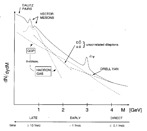
Let us briefly discuss the various sources of production of photons and dileptons during various stages of an URHIC and the specific domains of phase space where they are known to dominate. Let us first consider real photons. In the low transverse momentum region the contribution from pseudoscalar meson decays involving and clearly dominate photon production. In fact they account for nearly 95 of the total photon yield in a collision. Photons emitted due to primary interactions among the partons of the colliding nuclei form the principal background in the large transverse momentum region. These are called prompt or QCD photons. The decay photons can be isolated experimentally by invariant mass analysis and the prompt ones can be accurately estimated by perturbative QCD calculations. These contributions are then subtracted out to get the thermal photon spectra. Thermal photons from the QGP phase arise mainly due to the QCD Compton and annihilation processes. The emission rate resulting from these reactions turn out to be infra-red divergent and can be evaluated [55, 56, 57] in the framework of Hard Thermal Loop (HTL) [58, 59] resummation in QCD. The hadronic matter is mainly composed of the pseudoscalar-isovector pion () and the spin-isospin vector rho () mesons. One also includes the vector-isoscalar omega (), the pseudoscalar-isoscalar eta () and the axialvector-isovector mesons. Photons from the hadronic matter are emitted from reactions of the type (where is one of the hadrons , and ) as well as from the decay of short-lived hadrons [55]. In a phase transition scenario these are emitted during the later stages of the collision when the system has cooled to temperatures below . Hence the photon spectra due to the thermal hadronic phase is expected to have a steeper slope compared to the QGP. In Fig. (1.3) we have schematically shown the different contributions to the overall photon yield in a relativistic collision of heavy ions as a function of the transverse momentum of the emitted photons. One observes that the higher the transverse momentum of the photon the earlier they are produced in the collision process.

The different contributions to the production of lepton pairs as a function of their invariant mass are shown schematically in Fig. (1.4). The principal source of thermal dileptons from the QGP and hadronic phases are the quark-antiquark and pion annihilation processes respectively. In the high mass region these compete with Drell-Yan pairs which are produced in primary interactions between incoming partons in the very early stages of the collision. The peak marks the cut-off scale for thermal pairs from the plasma. Around this region the decays of and mesons also become an important source. The vector mesons which decay both during the expansion and after freeze-out can be identified easily from their characteristic peaks in the spectrum. Below the vector mesons, Dalitz decays of , , and mesons provide the dominant source for dilepton production. The fact that higher mass lepton pairs are produced earlier in the collision process is evident from the time axis in Fig. (1.4). We emphasize that whereas the dileptons from hadronic matter have distinct features like the , and peaks, the photon spectra is completely structureless. Hence it is very difficult to disentangle the thermal photons emitted from hadronic matter from those which have their origin in quark matter. In this case an accurate estimation of thermal photons originating from hadronic matter is of utmost importance in order to comment on the formation of QGP in relativistic heavy ion collisions. Such an estimation must incorporate medium modifications of hadronic properties in the evaluation of emission rates as well as in the equation of state (EOS) of the interacting hadronic matter. The change in the mass and decay width of a vector meson propagating in a medium occurs due to its interaction with the real and virtual excitations in the medium. Medium induced modifications of the properties of vector mesons, for example, the and are likely to show up clearly in the invariant mass spectra of dileptons through the shifting and/or broadening of the respective peaks. In the following Section we will give a brief introduction to the study of hadronic properties in a thermal medium.
1.4 Medium Effects on Hadronic Properties
In URHICs hadronic matter is expected to be formed after a phase transition from QGP when the plasma has cooled beyond the phase transition temperature . Even if such a phase transition does not occur, realization of hadronic matter at high temperature ( 150 – 200 MeV) and/or baryon density (a few times normal nuclear matter density) is inevitable. As a result the study of hadronic interactions at high temperature and density assumes great significance. However, progress in our understanding of hot and dense hadronic matter has been retarded since the underlying theory of strong interaction, QCD, is nonperturbative in the low energy regime. This severe constraint has lead to considerable amount of work on model building [61, 62, 63, 64] in order to study the low energy hadronic states.
The principal contention of this thesis is to study the medium effects on thermal photon and dilepton spectra. We will be mainly concerned with the vector mesons and . Various investigations have addressed the issue of temperature and density dependence of hadronic spectra within different models over the past several years. According to Brown and Rho [65] the requirement of chiral symmetry (in particular the QCD trace anomaly) yields an approximate scaling relation between various effective hadronic masses, which implies that all hadronic masses decrease equally with temperature. The reduction in meson mass has also been observed in the gauged linear sigma model [66] at low temperature; however, near the chiral transition point it shows an upward trend. The nonlinear sigma model claimed to be the closest low energy description of QCD shows the opposite trend, i.e. the effective mass increases with temperature [67]. A similar qualitative behaviour of the mass has been observed in the hidden local symmetry approach [68]. The relation between the self energy and the forward scattering amplitude has also been utilized to study the change of hadronic properties in the medium [69, 70], where the effects of non-zero temperature is rather small.
In the Quantum Hadrodynamic Model (QHD) of Walecka [71, 72] scalar and vector condensates generated by the nucleon sources are themselves responsible for the modification of the nucleon mass. The vector meson mass gets shifted due to the decrease of the nucleon mass which appears through thermal loops in the vector meson self energy [73], the imaginary part of which characterizes the response of the nuclear system to external (electromagnetic) probes.
In-medium QCD sum rules are useful to make constraints on the hadronic spectral functions at finite temperature and density [74]. In the QCD sum rule approach the hadronic properties are related to the scalar and tensor condensates of quark and gluon fields. Due to lack of understanding of the behaviour of these condensates near the critical point, the hadronic properties at finite temperature in this approach is not firmly established. The spectral function of vector mesons can be parametrized in vacuum from the experimental data obtained in (or from hadronic decays of the lepton) for various isovector and isoscalar channels [75, 76]. The in-medium spectral function of the vector meson is then obtained by modifying the pole and the continuum structure as a result of its interaction with the constituents of the thermal bath. The vector meson masses and the continuum thresholds are taken to vary with temperature according to Brown-Rho (BR) and Nambu scaling [77] scenarios.
So we see that a wide range of variation of hadronic properties with temperature are predicted by the models cited above. Other models e.g., those proposed by Rapp et al [78] and by Klingl et al [79], where the effects of non-zero baryon density (baryonic chemical potential) is dominant over non-zero temperature will not be discussed. This is because we intend to study the hot baryon free (central rapidity) region of URHICs. We shall consider various scenarios for the shift in the hadronic spectral function at finite temperature and evaluate its effects on the experimentally measurable quantities, the photon and dilepton spectra originating from a thermalized system formed in URHICs.
1.5 Organization of the Thesis
The thesis is organized as follows. In Chapter 2 we shall discuss the formalism of photon and dilepton production from a medium of interacting particles at finite temperature and/or density starting from first principles using perturbation theory. The rates of photon production from partonic interactions in the QGP as well as from hard primary interactions of partons will be considered. Chapter 3 is devoted to the study of spectral modifications of vector mesons in the medium and the evaluation of static (fixed temperature) rates of photon and dilepton production from hadronic matter within various models. The medium masses of the vector mesons are calculated from the pole positions of the effective propagators which are obtained in terms of the self energies calculated in the framework of thermal field theory using a few well-known models. We have considered the QHD model, the gauged linear sigma model, the gauged non-linear sigma model, and the hidden local symmetry and QCD sum rule approaches. The space-time evolution of these static rates using relativistic hydrodynamics is discussed in Chapter 4. The medium effects in the space-time evolution enters through the equation of state which is manifested in the cooling rate as well as in the estimation of the initial temperature of the produced matter. The final photon multiplicity with and without a QGP in the initial state is obtained. These are compared with data obtained by the WA80, WA98 and CERES experiments. Chapter 5 contains the thesis summary and related discussions. We have listed the invariant amplitudes of all the photon producing hadronic reactions and decays that we have used in the Appendix.
Chapter 2 Formulation of Electromagnetic Emission Rates
Electromagnetically interacting particles - photons and dileptons are excellent probes of the thermodynamic state of evolving strongly interacting matter likely to be produced in ultra-relativistic nucleus-nucleus collisions. This is because electromagnetic interactions are strong enough to lead to a detectable signal and yet are weak enough to let the emitted photons and leptons escape from the finite nuclear system without further interactions. Hence the spectra of photons and dileptons can provide information of the properties of the constituents from which they were emitted.
For most purposes the emission rates of photons and dileptons can be calculated in a classical framework. It was shown by Feinberg [80] that the emission rates can be related to the electromagnetic current correlation function in a thermalized system in a quantum picture and, more importantly, in a nonperturbative manner. Generally, the production rate of a particle which interacts weakly with the constituents of the thermal bath (the constituents may interact strongly among themselves, the explicit form of their coupling strength is not important) can always be expressed in terms of the discontinuities or imaginary parts of the self energies of that particle [81, 82]. In this Chapter we will make a detailed study of the connection between the emission rates of real and virtual photons and the spectral function of the photon which is connected with the discontinuities in self energies in a thermal system [83]. This in turn is connected to the electromagnetic current correlation function [50] through Maxwell equations. Alternatively, using the kinetic theory approach the photon emission rates can be written in terms of the equilibration rate of photons in a thermal bath. The imaginary part of the photon self energy tensor in this case is related to the exclusive kinetic rates of emission and absorption in the system. We will discuss these facets regarding the formulation of the photon and dilepton emission rates from a thermal medium extensively in Section 2.2 after a brief review of propagators in thermal field theory in Section 2.1. The invariant rates of emission of both hard and soft thermal photons and dileptons from QGP will be dealt with in Section 2.3 where we will compare the static (fixed temperature) rates due to different processes contributing to the thermal yield.
2.1 Review of Thermal Propagators
As is well known, propagators play a central role in the description of the dynamics of systems of particles using quantum field theory. In this Section we will briefly discuss the in-medium (thermal) propagators in Thermal Field Theory [82, 84, 85, 86] which will be used extensively in the thesis. We will begin by first defining the propagators in vacuum.
The free propagator of a complex scalar field propagating with a momentum in vacuum is defined as
| (2.1) | |||||
The operator appearing within angular brackets ensures that the field operators are time-ordered and the subscript ‘0’ indicates that there are no interactions. The vacuum propagator for fermions is defined as
| (2.2) | |||||
where and denote the spinor indices of the fermion field . In a similar way the free propagator of a vector field is defined as
| (2.3) |
Depending on the nature of the quanta of the vector field the vector propagator can take the following forms. In the case of a vector particle of mass we get
| (2.4) |
which describes the free propagation of the meson, for example. For charged vector particles e.g. the meson, the fields also carry isospin indices and we have
| (2.5) |
where and denote components in isospin space. In the case of massless vector fields corresponding to photons or gluons the propagator will contain a gauge parameter as a reminder of the arbitrariness of the gauge-fixing condition. The photon propagator in vacuum is obtained as
| (2.6) |
Some well known choices are, which is the Feynman (or Lorentz) gauge and , the Landau gauge. For gluons we need to add a Kronecker delta is colour space so that the free gluon propagator is
| (2.7) |
The gauge parameter must be absent from any physical quantity we calculate.
It must be noted that the fields , and appearing above are free fields and the expectation values are calculated between noninteracting vacuum states. The propagators defined through Eqs. (2.1), (2.2) and (2.3) are referred to as Feynman propagators.
In the presence of interactions these propagators have to be redefined with interacting Heisenberg fields in place of the free fields and interacting vacua instead of the free vacua. The interacting propagator can be expressed in terms of the bare (non-interacting) propagator using perturbation theory. In the scalar case, for example, the exact propagator in the presence of interactions, , is obtained as
| (2.8) |
Where, is the self energy of the particle due to interactions. This equation is known as the Dyson-Schwinger equation for propagators.
Let us now study the situation in a medium at finite temperature (and density). We will be interested in a system in thermal equilibrium. Hence we will assume that the interaction slowly switches off as we go into the remote past and the fields become noninteracting fields satisfying the free equations of motion. These fields appear in the definition of the free propagators in the medium. The thermal propagator has more structure than the vacuum case as a result of different combinations of time-ordering on the real time contour [82, 84, 102]. In the real time formalism there are four non-trivial propagator structures possible which are collected in a 22 matrix [87, 88]. For scalars the free thermal propagator is defined as
| (2.11) | |||||
| (2.14) |
where the operator denotes anti-time-ordered product. The subscript ‘’ indicates that a thermal average is being performed.
In order to obtain the thermal propagators in momentum space one follows the usual procedure of expanding the field operators in terms of the creation and annihilation operators and making use of the commutation relations between them. The four components are then obtained as
| (2.15) |
where . is the Bose distribution with , is the four velocity of the thermal bath and is the chemical potential. We observe that the elements of the matrix propagator are not independent. From their definitions one can see that and can be expressed in terms of and . Also, the Kubo-Martin-Schwinger [89] periodicity condition yields .
Similarly, for fermions the corresponding thermal propagators are,
| (2.18) | |||||
| (2.21) |
Explicitly, the four components are
| (2.22) |
where, , , the Fermi-Dirac distribution. For the fermions the KMS anti-periodicity condition leads to .
Lastly, we define the finite temperature propagators for vector particles:
| (2.25) | |||||
| (2.28) |
As before, one will have additional indices corresponding to colour or electric charge; henceforth we will not mention them explicitly. Apart from the Lorentz indices, the explicit forms of the thermal propagators will be similar to the scalar case. For neutral particles, the chemical potential will be absent in the definition of the phase space factor .
It is important to note that the real time propagators as given by Eqs. (2.15) and (2.22) consist of two parts - one corresponding to the vacuum, describing the exchange of virtual particles and the other, the temperature dependent part, describing the participation of real (on-shell) particles present in the thermal bath in the emission and absorption processes. The temperature dependent part does not change the ultra-violet behaviour of the theory as it contains on-shell contributions and has a natural cut-off due to the Boltzmann factor. Therefore, the zero temperature counter term is adequate for the renormalization of the theory. However, the infra-red problem becomes more severe at finite temperature [82, 90].
Thermal field theory in the real time approach can be reformulated by diagonalizing the 22 matrix propagators described above. A well-known possibility is to diagonalize to a matrix constructed from the Feynman propagators [87]. The free thermal propagator defined by Eq. (2.14) can be written as
| (2.29) |
where
The exact propagators in the medium can be defined analogously as Eqs. (2.14), (2.21) and (2.28) with interacting Heisenberg fields instead of the free fields. In this case we write
| (2.30) |
where is the matrix of interacting thermal propagators. Using thermal perturbation theory can be expressed in terms of . One obtains
| (2.31) |
where now is the self-energy matrix;
| (2.32) |
Matching the elements appearing in the diagonal of Eq. (2.31) we have
| (2.33) |
From Eq. (2.32) it also follows that
| (2.34) |
and
| (2.35) |
In the following we will discuss the vector (spin 1) propagator in some detail. It is very similar to the scalar case except now one has to take into account the Lorentz structure of the propagator and the self energy. The exact propagator (matrix) can be diagonalized as above and the diagonal element satisfies Dyson equation
| (2.36) |
which gives
| (2.37) |
where is the vacuum propagator for vector particles. The quantity is the sum of all one particle irreducible (1PI) self energy insertions. In has a vacuum and a medium part so that
| (2.38) |
where
| (2.39) |
is the vacuum contribution to the self energy.
Naively, it would appear that finite temperature corrections to quantum field theory breaks Lorentz covariance since the rest frame of the heat bath selects out a specific frame of reference. However, by defining a fluid four-velocity with temperature defined in the fluid rest frame where , a manifestly covariant formulation can be achieved [84, 91]. Using the techniques of tensor decomposition it can be shown that for a vector particle propagating with four-momentum ,
| (2.40) |
where and are Lorentz invariant self-energy functions which characterize the transverse and longitudinal modes. and are the transverse and longitudinal projection tensors given by
| (2.41) |
and
| (2.42) |
which satisfy the following algebra:
| (2.43) |
The two functions and are obtained by contraction:
| (2.44) |
Now, for massive vector particles,
| (2.45) |
Using Eqs. (2.37-2.43) the effective propagator becomes
| (2.46) |
where
| (2.47) |
and , we recall, is the bare mass of the particle. The real part of affects the dispersion relation of the particle in the medium. The displaced pole position of the effective propagator in the rest frame of the propagating particle (i.e. where the three momentum of the particle is zero) gives the effective mass of the particle in the medium. The imaginary part of is connected to the decay width.
A different scheme in the formulation of finite temperature field theory known as the ‘R/A’ formalism [92], is to diagonalize to a matrix composed of retarded and advanced propagators which are known to have better analyticity properties than the Feynman ones. In this case the analogue of Eq. (2.29) is
| (2.48) |
The free retarded and advanced propagators are defined as
| (2.49) | |||||
The matrices and depend on the momentum as well as the thermal factor containing the distribution functions. Their exact forms are given in Ref. [92]. For the case of massive vector particles one arrives at the following equation for the effective retarded propagator at finite temperature:
| (2.50) |
where and are respectively the retarded transverse and longitudinal components of the self energy. For photons we have [57]
| (2.51) |
Before we end our discussion of finite temperature propagators let us briefly mention about the imaginary time formalism or Matsubara formalism which has been used extensively in the literature. In the imaginary time formalism, the form of the propagator at finite temperature is the same as that in vacuum but the time component of the four-momentum takes discrete values, i.e. for bosons (fermions) with to , the vertices are the same as the zero temperature theory and the loop integral is replaced by the sum . There are standard methods to evaluate the sum over the frequencies [82]. The propagators in the imaginary time formalism can also be obtained by proper analytic continuation of the real time propagators [93, 94]. Another method, known as the SACLAY method has also been used extensively in the literature [58, 95]. This method uses the mixed representation of the propagator i.e. it depends on the three-momentum and Euclidean time.
2.2 Thermal Emission Rates
We note at the onset that the nature of emission of real and virtual photons depends crucially on the size of the hot thermal system from which they are emitted. If the system is large enough the photons will rescatter and thermalize and their momentum space distribution will be given by the Planck distribution. The corresponding emission rate will then be that of black body radiation which depends only on the temperature and the area of the emitting body but not on its microscopic properties. Since the typical size of systems produced in heavy ion collisions is much less than the mean free path of the photons, they are likely to escape the hot zone without rescattering and the emission rate in this case depends on the dynamics of the thermal constituents through the imaginary part of the photon self energy. We will begin by demonstrating this in a kinetic theory framework [60, 81] before going on to a more rigorous scheme. We will in general denote the four-momenta of the real and virtual photons by and respectively.
2.2.1 Emission Rate as Equilibration Rate
We know that the probability of a photon of 4-momentum to be absorbed in matter is given by
| (2.52) |
and the probability of emission is given by
| (2.53) |
Here, is the equilibrium distribution function, and denote the initial and final state particles, and denotes the phase space integration including spin and polarization sums. Now,
| (2.54) |
where the squared matrix elements of the forward and backward processes have been taken to be equal on account of time reversality. If is the momentum distribution function of photons, the rate of decrease due to absorption is and the rate of increase due to emission is . So the time evolution equation for is
| (2.55) |
The solution of this equation is
| (2.56) |
where, is the equilibration rate, is the Bose distribution function and is a function which depends on the initial conditions. Since the system under consideration is small enough for the photons to escape immediately on production, we must have . Consequently, Eq. (2.55) reduces to
| (2.57) |
Now, the equilibration rate is related to the imaginary part of the photon self energy through [96]. For a real photon and we have from Eq. (2.44), . Using
for a real photon we get from Eq. (2.57)
| (2.58) |
The quantity contains information about the constituents of the thermal bath and thus is of great relevance. After this relatively simple but illuminating exercise, we will proceed to arrive at this result from more general considerations in the following.
2.2.2 Emission Rate and Photon Spectral Function
We begin our discussion with the dilepton production rate. Following Weldon [83] let us define as the exact Heisenberg photon field which is the source of the leptonic current . To lowest order in the electromagnetic coupling, the scattering matrix element, , for the transition is given by
| (2.59) |
where is the initial state corresponding to the two incoming nuclei, is the final state which corresponds to a lepton pair plus the rest of the interacting system. The parameter is the renormalized charge which couples the leptonic current with the virtual photon field . Since we assume that the lepton pair does not interact with the emitting system, the matrix element can be factorized as
| (2.60) |
where is the vacuum state. Putting where is the field operator for the leptons, one obtains the expectation value in terms of the Dirac spinors and as
| (2.61) |
where denote the Dirac matrices, , with are the energies of the leptons and is the volume of the system. Therefore,
| (2.62) |
The leptons of four-momenta and are produced from a single virtual photon of four-momentum so that and .
Assuming that a thermalized system is produced in the collision, the dilepton multiplicity is obtained by summing over the final states and averaging over the initial states with a weight factor ;
| (2.63) |
where is the total energy in the initial state, is the partition function and is the inverse temperature. After some algebra can be written in a compact form as follows:
| (2.64) |
where is the leptonic tensor defined by
| (2.65) | |||||
and is the photon tensor
| (2.66) |
Using translational invariance we can write
| (2.67) |
where is the four-momentum operator and and are the total four-momenta of the initial and final states respectively. We now have
| (2.68) |
Using the conservation of four-momentum, and the completeness relation we get
| (2.69) |
where is the four-volume of the system and is the component of the exact photon propagator defined in the last Section. The time ordered propagator is the component of . In coordinate space it is defined as
| (2.70) | |||||
where is the component , is the time component of the four vector, and is the step function. Using the integral representation of the -functions,
and taking the Fourier transform we get [97]
| (2.71) |
Using the Kubo Martin Schwinger (KMS) relation in momentum space,
| (2.72) |
we have
| (2.73) |
The rate of dilepton production per unit volume () is then obtained as
| (2.74) |
Now, the spectral function of the (virtual) photon in the thermal bath is defined as
| (2.75) |
| (2.76) |
where . This leads to
| (2.77) |
In terms of the photon spectral function the dilepton emission rate is obtained as
| (2.78) |
This relation which expresses the dilepton emission rate in terms of the spectral function of the photon in the medium is an important result. Inserting,
and using the identity
| (2.79) | |||||
the dilepton rate () can be expressed as
| (2.80) |
where is the lepton mass and denotes the fine structure constant. We will now proceed to evaluate the photon spectral function.
As is well known, it is not the time-ordered propagator that has the required analytic properties in a heat bath, but rather the retarded one. We thus introduce the retarded propagator which will enable us to express the dilepton rate in terms of the retarded photon self energy. The retarded photon propagator in momentum space is defined as
| (2.81) |
which leads to the relations
| (2.82) |
and
| (2.83) |
The above equation implies that in order to evaluate the spectral function at we need to know the imaginary part of the retarded propagator. We note that the above expression for spectral function reduces to its vacuum value as since the only state which enters in the spectral function is the vacuum [98].
Now, as mentioned before, the exact retarded photon propagator can be expressed in terms of the proper self energy through the Dyson-Schwinger equation:
| (2.84) |
where, is the sum of all 1PI (one particle irreducible) retarded photon self energy insertions which can be decomposed as
| (2.85) |
Here and , as defined in the previous Section are the transverse and longitudinal projection tensors respectively and and are the transverse and longitudinal components of the retarded photon self energy. The presence of the parameter indicates the gauge dependence of the propagator. Although the gauge dependence cancels out in the calculation of physical quantities, one should, however, be careful when extracting physical quantities from the propagator directly, especially in the non-abelian gauge theory.
Inserting the imaginary part of the retarded photon propagator from Eq. (2.84) in Eq. (2.83) we get
| (2.86) |
where
| (2.87) |
Using,
| (2.88) |
the dilepton rate is finally obtained as
| (2.89) |
This is the exact expression for the dilepton emission rate from a thermal medium of interacting particles. It has been argued by Weldon [99] that the electromagnetic plasma resonance occurring through the spectral function at could be a signal of the deconfinement phase transition provided the plasma life time is long enough for the establishment of the resonance.
Since and are both proportional to (the fine structure constant) they are small for all practical purposes. Neglecting and in the denominator of Eq. (2.87) one obtains
| (2.90) |
This corresponds to the free propagation of the virtual photon in the thermal bath. Using Eqs. (2.89) and (2.90) we get
| (2.91) |
This is the familiar result most widely used for the dilepton emission rate [82]. It must be emphasized that this relation is valid only to since it does not account for the possible reinteractions of the virtual photon on its way out of the bath. The possibility of emission of more than one photon has also been neglected here. However, the expression is true to all orders in strong interaction.
2.2.3 Emission Rate and Current Correlation Function
The emission rate of dileptons can also be obtained in terms of the electromagnetic current correlation function [50]. We denote the electromagnetic current of the strongly interacting particles (quarks or hadrons) by the operator and the leptonic current by . As before, is the coupling between and the virtual photon. For the present, the current is taken to contain the coupling constant. The matrix element for dilepton production is
| (2.92) |
where is the free photon propagator. As in the earlier case the leptonic part of the current can be easily factored out and we get Eq. (2.61). The photon propagator is written in momentum space as
| (2.93) |
to obtain
| (2.94) |
Squaring the matrix elements and using Eq. (2.63) one obtains the rate of dilepton production
| (2.95) |
where is the Fourier transform of the electromagnetic current correlation function defined as
| (2.96) |
Note that this definition is different from that of Mclerran and Toimela [50] where
The correlation function is symmetric in and . One can use translational invariance and the KMS relation to show that
In this case the dilepton rate is
as in Ref. [50].
It is seen from Eq. (2.95) that from the measured dilepton and photon distributions the full tensor structure of can in principle be determined. This will yield considerable information about the thermal state of the strongly interacting system.
Now, is related to the retarded correlator by
| (2.97) |
where
| (2.98) |
Using the identity Eq. (2.79) and the transversality of the correlation function, the dilepton emission rate is obtained as
| (2.99) |
We now define the improper photon self energy through the relation
| (2.100) |
where is the sum of all self energy diagrams. The advantage is that can be defined in coordinate space as [100]
| (2.101) |
Taking the Fourier transform and comparing with Eq. (2.98) we see that
| (2.102) |
Therefore, the dilepton rate can also be expressed as [101]
| (2.103) |
It is important to realize that the analysis is essentially nonperturbative up to this point. To we note that reduces to the proper self energy () and consequently Eq. (2.103) reduces to Eq. (2.91). This approximation is the same as implied in Eq. (2.90).
Let us now try to relate the approach discussed in this Section with the previous one. We know that the equation of motion of the photon field is given by the Maxwell equation
which has the formal solution
where is the free photon propagator. This can be used in Eq. (2.59) to get Eq. (2.92). Again, the connection between the electromagnetic current correlation function and the spectral function can be expressed in a straight forward way by substituting and from the Maxwell equation in Eq. (2.96) to obtain
| (2.104) | |||||
The gauge dependent terms will not contribute due to current conservation and we have
| (2.105) |
Substituting this in Eq. (2.95) we can recover Eq. (2.78). This establishes the connection between the approaches of Refs. [83] and [50].
Let us now consider real photon emission from a system in thermal equilibrium. The matrix element is given by
| (2.106) |
where, is the electromagnetic current of the strongly interacting particles which produces the photon and is the free photon field. Since the photon escapes without re-interacting, the matrix element can be taken to factorize as,
| (2.107) |
In the case of a single photon of four-momentum the free field can be expanded as
| (2.108) |
so as to obtain
| (2.109) |
The thermally averaged photon multiplicity is given by
| (2.110) |
The sum over the photon polarization is performed using . Proceeding as before we obtain the photon emission rate as
| (2.111) |
Note that this expression also follows from the dilepton emission rate given by Eq. (2.95) with a few modifications. The factor which arises from the lepton spin sum of the square modulus of the product of the electromagnetic vertex , the leptonic current involving Dirac spinors and the square of the photon propagator is to be replaced by the factor from the polarization sum. The factor follows from the normalization of the photon field (Eq. (2.108)). Finally the phase space factor for the lepton pair, is replaced by .
Using Eqs. (2.97) and (2.102) and the fact that to lowest order in the improper and proper photon self energies are equal, we get
| (2.112) |
In this form, the real photon emission rate is correct up to order in electromagnetic interaction but exact, in principle, to all orders in strong interaction. However, for all practical purposes one is able to evaluate up to a finite order of loop expansion. It is clear from the above that in order to deduce the photon and dilepton emission rate from a thermal system we need to evaluate the imaginary part of the photon self energy. The Cutkosky rules at finite temperature or the thermal cutting rules [84, 102, 103] give a systematic procedure to calculate the imaginary part of a Feynman diagram. The Cutkosky rule expresses the imaginary part of the -loop amplitude in terms of physical amplitude of lower order ( loop or lower). This is shown schematically in Fig. (2.1). When the imaginary part of the self energy is calculated up to and including order loops where satisfies , then one obtains the photon emission rate for the reaction particles particles and the above formalism becomes equivalent to the relativistic kinetic theory formalism [104].
For a reaction the photon emission rate is given by [105]
| (2.113) | |||||
where
is the overall degeneracy of the particles 1 and 2, is the invariant amplitude of the reaction (summed over final states and averaged over initial states), denotes the distribution functions and , , are the usual Mandelstam variables. Now, the rapidity of a particle is defined as
where and are the energy and longitudinal momentum of the particle respectively. For massless particles the transverse momentum is
We then have , and in the case of real photons.
The dilepton emission rate derived above in terms of the photon self-energy can be connected by the optical theorem to the kinetic theory rate for a reaction which is given by
| (2.114) | |||||
where is the appropriate occupation probability for bosons or fermions. The Pauli blocking of the lepton pair in the final state has been neglected in the above equation. The transverse mass of the lepton pair is defined as where ; being the invariant mass of the lepton pair. Using the above definition of rapidity, we have , and . In terms of the cross-section for the production of a lepton pair the dilepton production rate can be expressed as
| (2.115) |
where
and
is the relative velocity of the colliding particles and .
2.3 Emission Rates from Quark Matter
In this Section we will discuss the rates of photon and dilepton emission from a thermal system composed of quarks, antiquarks and gluons at a temperature due to various processes which are known to contribute substantially to the yield from QGP. Since the constituents of the system are massless for all practical purposes, we will encounter infrared singularities in the evaluation of the rates. We will discuss how these can be screened by summing the Hard Thermal Loops (HTLs) [58, 59] in the theory. The yield due to the primary scattering of partons embedded in the colliding hadrons will also be discussed since they are expected to constitute the principal background to the thermal photons (dileptons) in the region of large transverse momentum (invariant mass).
2.3.1 Thermal Photon Emission Rates from QGP
Naively, one expects that the properties of QGP at high temperature () can be studied by applying perturbation theory due to the small value of the strong coupling constant, which is given by the parametrized form [106]
| (2.116) |
However, QCD perturbation theory at high temperature is plagued by infra-red problems and gauge dependence of physical quantities, e.g. the gluon damping rate [90, 107, 108]. The gauge dependence of the gluon damping rate was cured by Braaten and Pisarski [58] by an effective expansion in terms of hard thermal loops - i.e. including all the relevant loop effects in a given order of the coupling constant in a systematic way. The idea of HTL is based on the observation that at non-zero temperature there are two energy scales - one associated with the temperature , referred to as the hard scale and the other connected with the fermionic mass (), induced by the temperature, known as the soft scale. A momentum appearing in the self energy diagram of photon would be called soft (hard) if both the temporal and the spatial components are (any component is ). If any physical quantity is sensitive to the soft scale then HTL resummation becomes essential, i.e. in such cases the correlation function has to be expanded in terms of the effective vertices and propagators, where the effective quantities are the corresponding bare quantities plus the high temperature limit of one loop corrections.
However, the problem of infra-red divergences in QCD is not solved completely by the HTL framework. The quantities which are quadratically divergent in naive perturbation theory such as the damping rate of fast moving fermions in QGP becomes logarithmically divergent in effective perturbation theory. On the other hand quantities which are logarithmically divergent in the naive perturbation theory turns out to be finite if one applies HTL resummation method. The hard photon () emission rate which falls in the second category, is the relevant quantity for the present discussions.
The thermal photon emission rate from QGP is governed by the following Lagrangian density:
| (2.117) |
where
| (2.118) |

In the above, is the non-abelian field tensor for the gluon field of color , is the Dirac field for the quark of flavour , is the color charge, is the (fractional) electric charge of quark flavor , ’s are the Gell-Mann matrices, is the electromagnetic field tensor and is the photon field. As mentioned in the introduction, the dominant processes for photon production from QGP are the annihilation () and the Compton processes () as shown in Figs. (2.2a) and (2.2b) respectively. However, the production rate from these processes diverges due to the exchange of massless particles. This is a well-known problem in thermal perturbative expansion of non-abelian gauge theory which suffers from infra-red divergences. One type of the divergences could be cured by taking into account the ‘electric type’ screening through the HTL approximation [58]. The non-abelian gauge theory also contains ‘magnetic type’ divergences, which can be eliminated if there is a screening of the magnetic field [109, 110, 111]. This is in sharp contrast to Quantum Electrodynamics, which is free from screening of static magnetic field. However, the study of magnetic screening is beyond the scope of HTL approximation as the transverse component of the gluon self energy vanishes in the static limit in this framework. Magnetic screening is relevant if any physical quantity is sensitive to the scale , where all the loop contributions are of the same order [112] and hence the perturbation theory breaks down [113]. The production of soft photons () from QGP is non-perturbative because it is sensitive to the magnetic screening mass of the gluons [114] and consequently the soft photon emission rate is poorly known. The production of hard photons () is insensitive to the scale and hence infra-red divergences can be eliminated within the framework of HTL as discussed below.
Let us try to understand the notion of HTL using massless theory described by the Lagrangian density
| (2.119) |
The thermal mass (self energy) resulting from the one loop tadpole diagram in this model is . At soft momentum scale () the inverse of the bare propagator goes as . Thus, the one loop (tadpole) correction is as large as the tree amplitude. Therefore, this tadpole is a HTL by definition. Braaten and Pisarski [58] have argued that these HTL contributions should be taken into account consistently by re-ordering the perturbation series in terms of effective vertices and propagators. Therefore, according to their prescription we have
| (2.120) |
where is the counter term which should be treated in the same footing as the term. has been introduced in order to avoid thermal corrections at higher order which has already been included in the tree level. With the counter term the Lagrangian remains unchanged, so the effective theory is a mere re-ordering of the perturbative expansion. A similar exercise has to be carried out in gauge theory keeping in mind that an addition and subtraction of local mass terms will violate gauge invariance. The effective action for hot gauge theories have been derived in Refs. [115, 116, 117, 118, 119], whereas the authors of Refs. [120, 121] follow the classical kinetic theory approach for the derivation of the HTL contributions. It has been shown in Ref. [122] that the contribution of HTL to the energy of the QGP is positive. The counter term required to avoid double counting in evaluating the virtual photon production from QGP in the two-loop approximation has been derived in [123] recently.
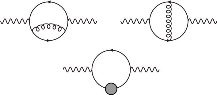
The photon emission from Compton and annihilation processes can be calculated from the imaginary parts of the first two diagrams in Fig. (2.3). Since these processes involve exchange of massless quarks in the channels the rate becomes infrared divergent. One then obtains the hard contribution by introducing a lower cut-off to render the integrals finite. In doing so, some part of the phase space is left out and the rate becomes cut-off dependent. The photon rate from this (soft) part of the phase space is then handled using HTL resummation technique. The application of HTL to hard photon emission rate was first performed in Refs. [55, 56]. For hard photon emission, one of the (soft) quark propagators in the photon self energy diagram should be replaced by effective quark propagators (third diagram in Fig. (2.3)), which consists of the bare propagator and the high temperature limit of one loop corrections [124, 125]. When the hard and the soft contributions are added, the emission rate becomes finite because of the Landau damping of the exchanged quark in the thermal bath and the cut-off scale is cancelled.
The rate of hard photon emission is then obtained as [55]
| (2.121) |
where is the strong coupling constant. Recently, the bremsstrahlung contribution to photon emission rate has been computed [57] by evaluating the photon self energy in two loop HTL approximation. The physical processes arising from two loop contribution (Fig. (2.4)) are the bremsstrahlung of quarks, antiquarks and quark anti-quark annihilation with scattering in the thermal bath. The rate of photon production due to bremsstrahlung process for a two-flavour thermal system with is given by [57]
| (2.122) |
and the rate due to annihilation with scattering in the thermal bath is given by,
| (2.123) |
where and . The most important implication of this work is that the magnitude of the two loop contribution comes out to be of the same order as those evaluated at one loop [55, 56] due to the larger size of the available phase space.
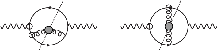
In case of soft thermal photon () emission, all the vertices and the propagators have to be replaced by the corresponding effective quantities. It has been shown [126, 127] that the result is divergent due to the exchange of massless quarks introduced through the HTL effective vertices itself. However, such collinear singularities for light-like external momentum could be removed with an improved action [119]. It is also shown that such infrared singularities could be removed through KLN (Kinoshita - Lee - Nauenberg) theorem [128, 129] by including appropriate diagrams and summing over all degenerate initial and final states [130, 131], but the rate is non-perturbative because it is sensitive to the scale [114].
The emission rate of hard photons is well under control within the framework of HTL resummation. However, there are important issues in hot gauge theories which cannot be addressed within the HTL resummation method [107, 132]. For example, (i) HTL resummation is based on the weak coupling limit () to distinguish between hard () and soft momentum scale () but such a limit may not be achievable in URHIC even for the highest energy to be available at the CERN LHC in the near future. Extrapolation of results obtained in HTL approximation to higher values of coupling constant will be demonstrated in Section 3.2 of Chapter 3 through the photon spectra. (ii) It cannot cure the infra-red divergence problem that arises in the damping rate of fast fermions, (iii) it cannot remove the mass shell singularities in the soft photon (real) emission rate, (iv) the next to leading order correction to the Debye mass diverges unless one includes magnetic screening, which is beyond the scope of HTL approximation and finally (v) HTL works for a system in equilibrium ; extension of the formalism to non-equilibrium processes is still in the early stages of development. Results from other methods such as ladder approximation [133], renormalization group equation [8] etc. will be very important in these cases.

We have studied soft (low transverse momentum) photon production due to parton bremsstrahlung in a thermal system within the soft photon approximation (SPA) [134]. These photons are produced from one of the external legs in a parton scattering diagram (Fig. (2.5)) i.e. due to processes like where is a quark or antiquark and can be a quark, antiquark or a gluon. These are hence processes compared to the processes described earlier. Naively, the soft photon approximation provides that the cross section for the process factorizes into a scattering part and a photon production part. The photon can be emitted from any of the external lines in Fig. (2.5). The emission of photons from the interior of the scattering vertex (the central blob in the figure) is neglected because in the limit of very low energy of the emitted photon its contribution is very small. The dependence of the photon momentum is neglected both in the strong part of the matrix element as well as in the phase space delta function. The latter is however taken care of through a correction factor. The matrix element is then written as
| (2.124) |
and the rate of production of soft thermal photons at temperature is given by
| (2.125) | |||||
where , and is the colour and spin degeneracy. The cross-section for the process is given by
| (2.126) |
with
| (2.127) |
Here is the real photon current and
| (2.128) |
where . The strong interaction differential cross-section and for scattering of quarks and gluons are obtained from semi-phenomenological expressions used earlier by several authors for this purpose.

The emission rates of hard and soft thermal photons are shown in Fig. (2.6). One observes that the 2-loop corrections to the photon rate namely, the bremsstrahlung contribution given by Eq. (2.122) (the long-dashed curve) and the contribution from annihilation with scattering as given by Eq. (2.123) (dot-dashed line) are of the same order as the 1-loop result (dotted line). Soft photons calculated in the SPA is plotted only up to 1 GeV for consistency [134] regarding the Landau-Pomeranchuk effect [135].
2.3.2 Hard QCD Photons
As remarked earlier, the large transverse momentum window for the photons will have a contribution due to partonic interactions which occur when nuclei start to interpenetrate at very high collision energy This contribution can be understood in terms of perturbative QCD, and can provide reliable information about the partonic distribution in the nuclei, as well as a means of providing near-absolute normalization of the photon measurements at larger transverse momenta. Since these photons are emitted at the very early stages of the collision with large momenta they are usually referred to as hard or prompt QCD photons. The cross section to leading order of perturbative QCD for the production of a photon in a hadronic collision, is obtained by convoluting the cross-section for the elementary processes e.g. Compton and annihilation with the gluon or quark contents of the participating hadrons [136]. Neglecting the correction due to neutron-proton asymmetry the nucleus-nucleus () collision is then built up as an incoherent sum of independent nucleon-nucleon () collisions. The cross section for the QCD Compton process at is given by
| (2.129) | |||||
where, and are the quark and gluon structure functions of the nucleon respectively and
For the annihilation process we have
| (2.130) | |||||
A large contribution to the prompt photons also comes from the fragmentation of partons in the final state in a parton-parton scattering, . These are bremsstrahlung processes and though of higher order () compared to Compton and annihilation ()), is found to contribute in the same order of magnitude at all values of the transverse momenta. Using an effective structure function the cross section for collisions is obtained as [136]
| (2.131) | |||||
where and
The strong coupling is given by
| (2.132) |
with , and GeV.
Neglecting the effects of shadowing, the photon distribution in a collision of nuclei and at an impact parameter due to hard scattering of partons is given by
| (2.133) |
where is the nuclear overlap integral. It is defined as
| (2.134) |
is the nuclear thickness function and is the nuclear number density normalized to the mass number . Also, is normalized such that
| (2.135) |
Let us now consider central () collisions of two identical nuclei of mass number . We will assume a constant nuclear number density , so that
and
Therefore,
Writing we obtain
| (2.136) |
In Fig. (2.7) we have plotted the photon yield due to the three processes described above using the MRSD- [137] set of structure functions. One observes that the yield from bremsstrahlung is of the same order as the sum of the Compton and annihilation processes. We have used in order to take into account the higher order QCD corrections.

2.3.3 Thermal Dilepton Emission Rates from QGP
The most dominant contribution to thermal dilepton production from QGP comes from quark anti-quark annihilation as shown if Fig. (2.2c). To obtain the differential number of lepton pairs emitted per unit four-volume we start from Eq. (2.115). Since quantum effects in the QGP is known to have a negligible effect we will use Boltzmann distribution for the quarks. The phase-space integrals are performed using the delta function to obtain
| (2.137) |
Integrating over we arrive at
| (2.138) |
and on integration over we get
| (2.139) |
The cross section for two light quark flavours can be evaluated using the diagram Fig. (2.2c) to obtain [22]
| (2.140) |
where is the lepton mass and is the quark mass. The thermal mass of the quarks will be used in the calculations. It is worth mentioning that the corrections to this rate comes from the Compton and annihilation diagrams i.e. the diagrams labelled and in Fig. (2.2) with a virtual photon in place of the real one [138]. One encounters mass (collinear) singularities in the evaluation of these processes which can be cured through the use of KLN theorem.
A significant contribution to the dilepton yield in the lower invariant mass region comes from soft (bremsstrahlung) processes. The rate of production of soft thermal dileptons can be evaluated analogously as the soft photons using the SPA. The photon emitted from the external lines in Fig. (2.5) in this case is a virtual one which eventually produces a lepton pair. The rate is given by [139]
| (2.141) | |||||
where
| (2.142) |
is as given in Eq. (2.127) with appropriately modified to account for virtual photon emission. The rates for thermal dilepton production from annihilation () is plotted in Fig. (2.8) along with the soft contributions discussed above.

2.3.4 Drell-Yan Dileptons
In the region of large invariant mass the dilepton yield is dominated by the Drell-Yan process and thus forms the principal background to dileptons emitted from the QGP. Here, a quark from one of the nucleons in nucleus annihilates an antiquark from one of the nucleons in the other nucleus to produce a virtual photon which subsequently decays into a lepton pair. The differential yield of such lepton pairs produced is collisions is obtained by an incoherent sum of the contributions from independent nucleon-nucleon collisions. For central collisions, the Drell-Yan yield is given by
| (2.143) |
where as in the case of prompt photons, and are the quark distribution functions of a nucleon. At , where is the square of the center of mass energy of the colliding nucleons.
2.3.5 Diphotons
We will briefly discuss the production of diphotons produced due to the annihilation of quarks and antiquarks. The importance of thermal diphoton emission lies in the fact that an experimental detection of large mass diphotons can possibly provide a valuable confirmation of the results obtained from the measurement of dileptons [140]. The diphoton cross section is given by:
| (2.144) | |||||
In the above , and is the charge of the quark and we have used . The emission rate is obtained by using this cross-section in Eq. (2.138) or Eq. (2.139). The rate of emission of thermal pairs from QGP at =200 MeV is shown in Fig. (2.8).

Diphotons with large invariant mass are also produced from the hard QCD annihilation of quarks and antiquarks in the colliding nuclei. The yield can be calculated analogously as the Drell-Yan pairs to get [140]
| (2.145) | |||||
At , . An arbitrary cut-off on the momentum transfer GeV) has been introduced so that perturbative QCD remains valid in this case. In Fig. (2.9) we have shown the dilepton yield due to the Drell-Yan process for Pb-Pb collisions at 200 A GeV. Also shown is an estimate of the diphoton yield in such a collision. As before we have used the MRSD- set of nucleon structure functions.
Chapter 3 Medium Effects and Emission Rates from Hot Hadronic Matter
In this Chapter we will consider photon and dilepton emission from a thermal system of interacting hadrons. We have seen that the photon and dilepton emission rates are related to the imaginary part of the photon self energy in the medium. As a result the rates will depend on the in-medium modifications of the hadrons appearing in the internal loop of the photon self energy diagram. Here the hadronic medium consists of mesons and baryons at a finite temperature. Due to the interactions with real and virtual excitations, the properties of these hadrons are expected to get modified. As a result the propagators appearing in the photon self energy undergo modifications. These are studied in the framework of Thermal Field Theory.
Many of the hadrons in a hot hadronic gas are electrically charged and hence couple to the electromagnetic field. Pions and mesons form the most important constituents of such a system. This is because pions are light and the mesons have large spin-isospin degeneracy. Lagrangian densities constructed with the , , , and fields have been used to calculate the amplitudes for photon production. Of these, the medium modifications of the and mesons are known to affect the photon and dilepton spectra significantly. Though we have included the presence of nucleons and antinucleons for the evaluation of the medium effects of vector mesons, we have neglected their contribution to the production of photons and dileptons. Also, we will assume the net baryon number to be zero. In Section 3.1 we will study the in-medium modifications of hadronic masses and decay widths using well known models. Thereafter, in Secs. 3.2 and 3.3 we shall discuss the emission rates of photons and dileptons where these medium modifications are taken into account.
3.1 Hadronic Properties at Finite Temperature
In this Section we will consider the in-medium modifications of the mass and decay widths of the and mesons. We will discuss the Quantum Hadrodynamic (QHD) model, the gauged linear and non-linear sigma models, and the hidden local symmetry approach. We will also show how the QCD sum rules can be used to constrain the spectral functions of the vector mesons in the medium.
The change in the hadronic mass in the medium can be understood from the following phenomenological arguments [141]. Let us consider the propagation of a vector meson in a nuclear medium. The attenuation of the amplitude at a distance , in a Fermi gas approximation, is given by , where is the density of nucleons and is the meson-nucleon interaction cross section. The optical theorem relates to the imaginary part of the forward scattering amplitude; . It then follows that the meson wave function , where the imaginary part of accounts for the attenuation and the real part modifies the dispersion relation of the propagating particle. In terms of an effective mass , the propagation can also be described by . Comparing the arguments of the exponential we get
| (3.1) |
This relation clearly shows that the enhancement or reduction of hadronic masses depends on the sign of .
3.1.1 Quantum Hadrodynamics
In the Quantum Hadrodynamic model [71, 72] of nuclear matter the vector meson properties are modified due to coupling with nucleonic excitations. The discussion has two parts. We will first study how the properties of nucleons are modified in matter at finite temperature. The nucleons interact through the exchange of scalar and the vector mesons and their mass is modified due to the scalar condensate. Thereafter, we will consider the changes in the and meson masses due to coupling with these modified nucleonic excitations.
a) The Nucleon Mass
The interaction in QHD is described by the Lagrangian
| (3.2) |
where , , and are the nucleon, , and meson fields respectively. The field couples to the scalar (vector) current of the nucleon with the coupling constant which will be specified later.
As discussed in the previous Chapter (Section 2.1), the free nucleon propagator at finite temperature and density in general has four components. The time-ordered i.e. the (11)-component is physically relevant for our purpose and we will denote this as where denotes the four-momentum of the nucleon. So we have
| (3.3) | |||||
where the first term () describes the free propagation of nucleon-antinucleon pairs and the second term () allows for the on-shell propagation of particle-hole pairs. in the above equation is the free nucleon mass.
The effective mass of the nucleon in matter at finite temperature in presence of the interaction described by Eq. (3.2) will appear as a pole of the effective nucleon propagator. In the Relativistic Hartree Approximation (RHA) [71, 72] one obtains the effective propagator by summing up scalar and vector tadpole diagrams self-consistently i.e. by using the interacting propagators to determine the self energy. The effective propagator referred to as the Hartree propagator is given by
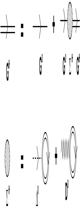
| (3.4) |
This is pictorially shown in Fig. (3.1). Here is the nucleon self energy which contains contributions from both scalar () and vector () tadpole diagrams [71, 72] and is given by
| (3.5) |
where
| (3.6) |
and
| (3.7) |
Here, is the mass of the neutral scalar (vector) meson. The solution of Eq. (3.4) now reads,
| (3.8) | |||||
One observes that the pole structure of the effective nucleon propagator in RHA resembles that of the non-interacting propagator with shifted mass and four-momentum i.e. and , is the effective mass. Using in place of the full Hartree propagator in Eqs. (3.6) and (3.7) defines the Mean Field Theory (MFT) values of the self energies. This is equivalent to solving the meson field equations with the replacement of the meson field operators by their expectation values which become classical fields i.e. and . This yields
| (3.9) |
which indicate that the nuclear ground state contains scalar and vector meson condensates generated by baryon sources. is the baryon density of the medium and is the (Lorentz) scalar density. The spatial part of the condensate vanishes due to rotational symmetry in infinite nuclear medium. These condensates are related to the scalar and vector self energies generated by summing tadpole diagrams in QHD as
| (3.10) |
The mean field approximation is thus to neglect the fluctuations in the meson fields which themselves are generated by the nucleons.
RHA is obtained when one includes the vacuum fluctuation corrections to the MFT results. This amounts to the inclusion of the Dirac part of the propagator in the calculation of the self energies. Summing over the vacuum tadpoles results in a sum over all occupied states in the negative energy sea of nucleons. Vacuum (or quantum) fluctuations, as these are called, form an essential ingredient in a relativistic theory of many particle systems. Since there are infinite number of negative energy states in the vacuum one expects that the vacuum contribution to the self energy is infinite.
Let us now find the Hartree self energy of the nucleon with the full nucleon propagator consisting of a medium as well as a vacuum part. The vector part of the self energy is obtained from Eq. (3.7) as
| (3.11) |
The first term of this equation appears to be divergent. The usual procedure is to regularize the integral in dimensions by dimensional regularization to render the integral finite. One can then shift the integration variable from to . The resulting integral vanishes by symmetric integration. The vector self energy then reduces to
| (3.12) |
and gives rise to a an effective chemical potential,
| (3.13) |
The scalar part of the self energy follows from Eq. (3.6):
| (3.14) | |||||
where
The baryon density of the medium is given by
| (3.16) |
The first term in Eq. (3.14), to be denoted by , represents the contribution to the scalar self energy from the filled Dirac sea and is ultraviolet divergent. We will now proceed to renormalize this divergent contribution. The first step is to isolate the divergent part through dimensional regularization. This gives
| (3.17) | |||||
since . The divergence in now appears as the pole of the -function for physical dimension . The counter terms needed to remove the divergent contributions from the loop corrections to the measurable amplitudes are
| (3.18) |
Including the contributions from the counter terms the renormalized self energy becomes
| (3.19) |
where
| (3.20) |
The coefficients () are fixed by defining a set of renormalization conditions. Since the scalar density (=) is not a conserved quantity the tadpole diagrams appear in the self energy. The tadpole contribution must vanish in normal vacuum (free space) i.e. . This is ensured by the term in . is the meson mass counter term which ensures that is the physical (measured) mass. Since the original Lagrangian of QHD [71] does not contain and terms, three and four point meson amplitudes must vanish at the tree level. The last two counter terms in Eq. (3.18) are chosen to maintain this condition at zero external momenta for the meson when nucleon loop corrections are included. We thus have
| (3.21) |
Consequently the effective nucleon mass reads
| (3.22) | |||||
The solution of this equation (with and MeV) gives the effective nucleon mass as a function of temperature and baryon density. At zero baryon density it can be parametrized as [142]
| (3.23) |
where is in GeV. We thus observe that in nuclear matter, scalar() and vector() mean fields induced by nucleon sources give back-reactions to the nucleon propagation itself and modify its self energy. This is the origin of in QHD.


In Fig. (3.2) we depict the variation of nucleon mass with temperature for a set of baryon densities. We observe that the nucleon mass falls steadily with density for a fixed temperature. However, the variation with temperature for given values of baryon densities shows interesting features. At zero baryon density the nucleon mass decreases monotonically as a function of temperature, but for finite densities it increases slightly before falling. This trend is similar to that obtained by Li et al [143], and may be attributed to the modification of the Fermi-sea at finite temperature and density. Our calculation shows a 35% reduction of the effective nucleon mass at = 160 MeV and two times normal nuclear matter density compared to its free mass. In order to highlight the effect of vacuum fluctuation corrections we compare the MFT results with those obtained using RHA. This is plotted in Fig. (3.3). We observe that the effect of vacuum fluctuation is substantial for higher values of the baryon density. The contribution of the antinucleons from the Dirac sea is responsible for such an effect.
b) The Vector Meson Mass
In a medium, meson properties get modified due to its coupling to nuclear excitations as shown in Fig. (3.4). This modification is contained in the meson self energy which appears in the Dyson-Schwinger equation for the effective propagator in the medium. The interaction vertices are provided by the Lagrangian
| (3.24) |
where , is the free nucleon mass, is the nucleon field and , being the Pauli matrices.

The lowest order contribution to the vector meson self energy is expressed in terms of the self-consistent nucleon propagator described in Eq. (3.8). This is given by
| (3.25) |
where represents the meson-nucleon vertex function obtained from Eq. (3.24) and is given by
| (3.26) |
where . The vector meson self energy can be written as a sum of two parts
| (3.27) |
where
| (3.28) | |||||
is the vacuum polarization. This is a bilinear function of and hence describes the correction to the meson propagators due to coupling to excitations. The pairs can be excited only if the four-momentum carried by the mesons is in the time-like region . Hence the shift in the mass of the vector mesons due to vacuum polarization is caused by processes like where represents nucleons in the modified Dirac sea having an effective mass , smaller than what it would be in free space. From Eqs. (3.28) and (3.8) we have
| (3.29) |
From naive power counting it can be seen that this part of the self energy is ultraviolet divergent and has to be renormalized. A few comments about renormalizability of the interaction given by Eq. (3.24) is in order here. At very large momenta the propagator for massless bosons , whereas for massive vector bosons it goes as . This poses severe problems to the renormalizability of the theory with massive vector bosons. However, in a gauge theory with spontaneous symmetry breaking the vector gauge bosons acquire mass in such a way that the renormalizability of the theory is always preserved. The theory which involves neutral massive vector bosons coupled to a conserved current is also renormalizable. This is because in a physical process the propagator appears between two conserved currents and and the offending term does not contribute because of current conservation , making the theory renormalizable. This is the case for the meson [144, 145] which we shall consider first. The counter term required in this case is
| (3.30) |
We use dimensional regularization to separate the divergent and the finite parts. The divergences now appear as a pole in the -function at the physical dimension . The renormalized vacuum polarization tensor for the is then given by
| (3.31) |
where
| (3.32) | |||||
in which the counter term contribution
| (3.33) |
has been included. is now determined by the renormalization condition
| (3.34) |
Finally, we arrive at
| (3.35) | |||||
Because of the tensor interaction in Eq. (3.24) the vacuum self energy for the meson is not renormalizable. We employ a phenomenological subtraction procedure [146, 147] to extract the finite part using the condition;
| (3.36) |
with ( 0,1,2,….). Using dimensional regularization and the above subtraction procedure we arrive at the following expressions:
| (3.37) |
where
| (3.38) |
| (3.39) |
The medium dependent part of the polarization, , describes the coupling of the vector mesons to particle-hole excitations. It contains at least one on-shell nucleon propagator which provides a natural ultraviolet cut-off in the loop momenta. This part of the self energy leads to an increased effective mass of the vector mesons in the medium.
We recall that in a hot and dense medium because of Lorentz invariance and current conservation the general structure of the polarization tensor takes the form
where the two Lorentz invariant functions and are obtained by contraction as
being the four velocity if the thermal bath.
In the case of a vector meson of four-momentum interacting with real particle-hole excitations in the nuclear medium these are obtained as
| (3.40) | |||||
with
| (3.41) | |||||
| (3.42) | |||||
and
| (3.43) | |||||
The longitudinal component of the polarization tensor is given by
| (3.44) |
with
| (3.45) | |||||
| (3.46) | |||||
and finally
| (3.47) | |||||
where and stands for Fermi-Dirac distribution functions for the nucleons. In the above the superscripts ‘’, ‘’ and ‘’ represent the vector-vector, vector-tensor and tensor-tensor components respectively arising from the product of vector and tensor terms in Eq. (3.26). The dispersion relation for the longitudinal (transverse) mode now reads
| (3.48) |

It is important to point out that the self-energy functions of the nucleon as well as that of the vector mesons calculated in this section are actually the 11-component of the 22 self-energy matrix in the real time formulation of thermal field theory. Since here we are concerned about the real(dispersive) part of the self-energy in our discussion on effective masses we do not make any distiction between these and the scalar self energy function following Eq. (2.34) of Chapter 2.
In Fig. (3.5) we plot the dispersion relations for and mesons at MeV and twice normal nuclear matter density. This is obtained by solving Eq. (3.48) for the and mesons. One observes a small difference between the longitudinal(L) and transverse(T) modes in case of the meson but in case of the this splitting is negligible (attributable to the smaller vector coupling constant). We have observed that the quantity along the dispersion curve remains almost constant which is defined as the value of at on the mass hyperbola. This means that a simple pole approximation of the and propagator at is good enough for our calculations. The splitting between the transverse and longitudinal components of the self energy of vector mesons with both vector and tensor interactions can be shown to be [148],
| (3.49) | |||||
where
The following values of the coupling constants and masses [144, 146] have been used in our calculations so as to reproduce the nuclear saturation density: , , MeV, MeV, , and .
Thus the physical mass is defined as the lowest zero of Eq. (3.48) in the limit . In this limit , and we have,
| (3.50) |
where
| (3.51) |
with
| (3.52) | |||||
and . The effective mass of the vector meson is then obtained by solving the equation:
| (3.53) |
The effective masses take the following parametrized forms [142]:
| (3.54) |

The effective mass of the meson has been estimated from that of the mass using Weinberg’s sum rule [149]. One finds reference to two other kinds of masses in the literature. The invariant mass is defined as the lowest order zero of Eq. (3.48) with neglected. Again, the screening mass of a vector meson is obtained from the pure imaginary zero of the quantity on the left hand side of the same equation with . These two masses are different because of the non-analyticity of the polarization tensor at the origin i.e. at ().

In Fig. (3.6) the effective mass of the meson is plotted against temperature for various values of baryon density. We observe that the variation of the mass follows qualitatively the same trend as that of the nucleon. In this case, the mass decreases by 45% at = 160 MeV and two times normal nuclear matter density compared to its free space value. This is due to the fact that the large decrease of the modified Dirac sea contribution to the self energy dominates over the in-medium contribution which is seen to increase with temperature. We then evaluate the effective mass with the values of the coupling constants mentioned above. The results are plotted in Fig. (3.7). The quantitative difference in the and meson masses is due to the different numerical values of the coupling constants e.g. the tensor interaction is absent in case of the meson and quite significant for the meson.
Before we proceed further a few comments on the QHD model calculations are in order. In this model the major contribution to the change in the masses of the and mesons arises from the nucleon-loop diagram. For the dressing of internal lines in matter we restrict ourselves to the Mean Field Theory (MFT) to avoid a plethora of diagrams and to maintain internal consistency. It has been shown [101, 105] that the change in the mass due to interaction is negligibly small at non-zero temperature and zero baryon density. Therefore the change in the meson mass due to interaction is neglected here. At finite baryon density, the dynamics is more involved due to the medium effects on the vertex, the pion propagator coupled with delta-hole excitation, and the coupling of the meson with -hole excitations [79, 150, 151, 152, 153, 154, 155, 156]. The effect of such medium modifications is to broaden the -peak as well as to produce complicated structure around the peak. Here we have restricted our calculations within the realm of MFT, i.e the internal nucleon loop in the and self energy is modified due to tadpole diagram only.
c) The Vector Meson Width

The physical decay width of an unstable particle is related to the imaginary part of its self energy. For a particle at rest the width is obtained from the relation
| (3.55) |
where is the energy of the decaying particle. There are various ways to calculate the imaginary part. The Cutkosky rules at finite temperature [84, 102, 103] provides a simple and systematic way to calculate the imaginary part of the self-energy. Again, use can be made of the fact that the self-energy function develops cuts along the real axis when the particles in the internal loop become on-mass shell. The discontinuity across these cuts is pure imaginary for real so that we have
| (3.56) |
Let us consider the meson width. The imaginary part of the self energy is totally dominated by the pion loop which is borne out by the fact that the two pion decay mode of the has a branching ratio of 100 %. In contrast, the real part of the self energy which is responsible for the mass modification has a negligible role to play as far as the pion loop is concerned. It is found to cause a small positive shift of the pole. The interaction is described by the Lagrangian
| (3.57) |
The 11-component of the self energy of the meson due to pion loop (Fig. (3.8))is given by
| (3.58) |
where the pion propagator is
After integration over , the imaginary part of the self-energy function is obtained as
| (3.59) | |||||
where use has been made of Eq. (2.35). Using the relations given in Eq. (2.44) the longitudinal and transverse components can now be worked out. The terms involving the thermal distribution functions in the above equation can be interpreted in terms of pion absorption from and emission into the medium. The first and second -functions correspond to time-like and space-like regions of respectively. Restricting to the time-like region, we define the spin-averaged quantity,
| (3.60) | |||||
where . In the rest frame of the () this reduces to
| (3.61) |
Using Eq. (3.55) the decay width is obtained as
| (3.62) |
with . It is interesting to note that the phase space factor when written in this form clearly shows that the in-medium width is actually the difference between the rates of decay and formation of the resonance.
In Fig. (3.9) we demonstrate the in-medium effect on the decay width of meson. The observed enhancement of the decay width with temperature at non-zero values of the baryon density is solely due to the stimulated emission of pions in the medium; a consequence of the terms in the decay width. This is just a manifestation of the well known Bose enhancement (BE) effect which is more clearly observed in Fig. (3.10).


The effect of the modifications in the mass and decay width of an unstable particle is conveniently illustrated through the dimensionless quantity which is basically the spectral function apart from some factors. It is defined as
| (3.63) |
where is the invariant mass of a lepton pair and . The spectral function , in units of is plotted in Fig. (3.11). The shifts in both the spectral functions towards the lower invariant mass region correspond to the reduction of their masses due to thermal interactions.
Let us now consider the meson. The vacuum width ( MeV) of the is known to be dominated by the mode. A substantial contribution to the width also comes from the process in a thermal bath [148, 157]. The Feynman diagrams are shown in Fig. (3.12).

We shall use the Gell-Mann Sharp Wagner (GSW) interaction [158] given by
| (3.64) |
for the vertex and the Lagrangian given by Eq. (3.57) for the vertex. The width is obtained as
| (3.65) |
where is the phase space factor, given by
and
The limits of integration are
and
where is the pion 3-momentum.

The amplitude for the process is
where
and
with
The contribution from the reaction to the decay width of the is calculated analogously.
In Fig. (3.13) we have shown how the decay width of the meson increases with temperature. The narrow peak of the in vacuum is broadened substantially due to interactions with the thermal pions. Both the modes discussed above are seen to contribute almost equally to a ten-fold broadening of the in the medium. This is also observed in the spectral function of the shown in Fig. (3.14) where and .

3.1.2 Models with Chiral Symmetry
In this Section we will discuss finite temperature effects on the vector meson properties considering a few models which respect chiral symmetry. The effects of in-medium properties of vector mesons on the electromagnetic probes will be presented in Section 3.2.
a) The Gauged Linear Sigma Model
The linear sigma model (LSM) is a convenient tool to describe the low energy dynamics of pions, because it shows explicitly how the spontaneous symmetry breaking (SSB) of global chiral symmetry (SU(2)SU(2)) by the isosinglet sigma field generates pions, the Nambu-Goldstone (NG) bosons. However, there are reservations about the description of the meson as a well-defined degree of freedom because of its large decay width which is comparable to its mass. But, it has been argued [44, 159] that in the limit of chiral symmetry restoration, the decay of into two pions should be disallowed as and become degenerate in mass in this limit. It has been explicitly shown that the width of due to decay vanishes as , where is the critical temperature for chiral transition. Though it is still not known whether or not the critical temperature for deconfinement and chiral transition are the same; presently we will make no distinction between them.
The simplest version of LSM contains isosinglet field and isotriplet pion field and respects the charge conjugation, parity and time reversal symmetry (CPT) [42]. The Lagrangian obeying these constraints is
| (3.66) |
where is defined as
| (3.67) |
with being the Pauli matrices. The non-zero value of ensures that the pions are massive and consequently PCAC (partially conserved axial current) relation is satisfied. Note that is chirally invariant. Elimination of the field by imposing the condition results in the Non-Linear Sigma Model, which will be discussed in the next Section.
In the gauged LSM [42, 66, 160] one introduces the vectors and their chiral partners (axial vector) through left and right handed fields as
| (3.68) |
| (3.69) |
where and are the chiral partners of the and mesons respectively and .
The inclusion of axial vector mesons will increase the number of possible couplings and hence the number of arbitrary parameters become large. In order to include vector mesons in LSM with minimal coupling to the matter fields and , one requires [161], that the Lagrangian and its chiral transformation properties are such that the current generated by the chiral transformation is proportional to the vector field itself. This leads to the field-current identities and eventually the idea of VMD [162]. The field-current identity is achieved by promoting the SU(2) global chiral symmetry of vector fields to a local gauge symmetry as was done by Yang and Mills [163] for the isospin symmetry. The Lagrangian for the vector field reads,
| (3.70) |
where . In the above Lagrangian the kinetic term for the gauge fields remains invariant under the transformation and the field-current identity is obtained through Gell-Mann Levy theorem from the mass term of the gauge fields as
| (3.71) |
We note that chiral symmetry is a global one in QCD. Therefore, the local symmetry has to be broken and this is achieved by the mass term of the vector fields in the Lagrangian. Next, one has to introduce the interaction of matter fields ( and ) and the gauge fields preserving the field-current identity. Noting that the ordinary derivatives occurring in Eq. (3.66) spoils the field-current identity, we introduce the required interactions consistent with the gauge principle i.e. by replacing the partial derivatives by covariant derivatives:
| (3.72) |
Finally the Lagrangian density for the gauged LSM is obtained from Eqs. (3.72), (3.66) and (3.70) as
| (3.73) |
Expanding the kinetic term for the matter field one finds
| (3.74) |
The above equation indicates that (i) a shift in the field () gives rise to mixing between and fields (a term arises from the second term of the r.h.s. of Eq. (3.74)), which has to be eliminated by an appropriate shift in the field, (ii)there is no interaction term involving , which can only be introduced through anomaly and (iii) the kinetic term for pion gets modified because of the shift in the field. Thus to get back the canonical form of this term one has to renormalize the pion field , where . gives the Kawarabayashi - Suzuki - Riazuddin- Fayyazuddin (KSRF) relation [164, 165]. After some algebra one gets [66],
| (3.75) |
Taking MeV, MeV, MeV and MeV, we get MeV, MeV)3, MeV and .
With these inputs the thermal masses of and mesons to lowest order in at low temperatures are obtained as [66]
| (3.76) |
| (3.77) |
In the chiral limit goes to zero and many of the couplings vanish. Assuming the validity of VMD in the medium Pisarski has showed that [166] and become degenerate with a mass value MeV (i.e. mass increases). On the other hand, if one adopts a scenario where vector meson dominance (VMD) is not valid in the medium then MeV ( mass decreases). However, it is important to mention at this point that chiral symmetry can also be realized via the Georgi limit [167] where the meson becomes massless. Pisarski [42] has argued that the results obtained by Georgi in the non-linear sigma model can be translated in terms of the gauged linear sigma model without the validity of VMD, for which there is no unique prediction for the behaviour of the mass at non-zero temperature. Thus the behaviour of in-medium depends on the validity of VMD in the medium.
b) The Gauged Non-Linear Sigma Model
It is well-known that the global symmetry of two-flavour QCD is expected to be spontaneously broken to the subgroup and the pions appear as the N-G bosons. The non-linear sigma model with is an effective theory of QCD for the description of pion dynamics. The in-medium properties of vector mesons have been studied by Song [67, 168] in the framework of gauged non-linear sigma model (NLSM) [61]. We will discuss this model briefly because it is very similar to the gauged LSM; the main difference is that the degree of freedom is eliminated in NLSM by the non-linear realization of chiral symmetry as mentioned in the previous Section. We start with the observation that a perfectly valid parametrization of the matter field could be
| (3.78) |
where is the pseudoscalar field and . The Lagrangian for the NLSM based on the manifold is given by
| (3.79) |
The vector and the axial vector fields can be introduced as the Yang-Mills gauge fields as before to minimize the number of arbitrary parameters in the model. The resulting Lagrangian is given by
| (3.80) | |||||
where , and denote vector and axial vector fields. To improve the phenomenology of the model, the following higher dimensional terms can be added to the Lagrangian [67, 169] without spoiling the symmetry under consideration
| (3.81) |
where is a constant determined form the decay of vector mesons [67]. The thermal shift of the -mass evaluated with pion loop, pion tadpole and pion- loop resulting from the interaction given by Eqs. (3.80) and (3.81) shows negligible change in the -mass from its vacuum value [67].
The effective masses of , and at non-zero temperature have also been evaluated [168] with a symmetric Lagrangian:
| (3.82) | |||||
where is defined as in Eq. (3.78) with the Pauli matrices replaced by the Gell-Mann matrices . The two higher dimensional terms with co-efficients and are added to improve the phenomenology. It may be noted that although these terms retain the gauge invariance of the model the renormalizability of the model is spoiled.
The dynamics of the meson is governed by the anomalous interaction, also known as Wess-Zumino interaction given by
| (3.83) |
This is very similar to the Gell-Mann Sharp Wagner [158] interaction already described before.
The following values of the parameters consistent with the vacuum properties of the vector and axial vector mesons have been considered [168]: and , referred to as set I and II respectively. The calculation of the thermal mass shift of the vector and axial vector mesons with these inputs reveal that: (i)for parameter set I and masses increase with different rate and mass decreases, (ii) for parameter set II the thermal mass shift of and is negligibly small but mass decreases slightly.
c) The Hidden Local Symmetry Approach
In case of the two chiral models described above the vector mesons are introduced as Yang-Mills field and the mass term for the gauge bosons are put in by hand which is not entirely satisfactory. In the hidden local symmetry (HLS) approach the meson is generated as a dynamical gauge boson of a hidden symmetry in the NLSM [170, 171]. It has been explicitly shown that, in general, any NLSM corresponding to the manifold is gauge equivalent to a “linear” model having symmetry. Accordingly, the Lagrangian of Eq. (3.79) can be written in a form that exhibits, besides global, a local symmetry - the hidden symmetry and the meson appears as a gauge boson corresponding to this symmetry. (The axial vector is not included in the minimal version of HLS Lagrangian.) To make it more explicit, one introduces two matrix-valued variables and with the transformation properties [170],
| (3.84) |
with
| (3.85) |
where and . is parametrized as
| (3.86) |
where and . The unwanted degrees of freedom , which have entered through Eqs. (3.85) and (3.86) are known as the “compensators”- the would be N-G bosons which have to be “eaten up” by the hidden gauge boson, . These extra degrees of freedom then reappear as the longitudinal polarization of the (massive) .
Now the covariant derivatives are defined as
| (3.87) |
where is the external field corresponding to the gauging of and is the gauge field corresponding to the symmetry . With these fields two types of invariants can be constructed [170, 171, 172] which are
| (3.88) |
A linear combination is equivalent to the original Lagrangian given in Eq. (3.79). By fixing the gauge and hence eliminating the unphysical degrees of freedom, ) one can show that while vanishes when the equation of motion for is used. So far, has been treated as an auxiliary field. It is assumed that the kinetic term for this field is generated by quantum effects or by QCD dynamics. The full Lagrangian with the kinetic term is
| (3.89) |
where is the non-abelian field tensor for the meson. The Lagrangian of Eq. (3.89) is then written as [170],
| (3.90) |
The above equation implies that the mass of the meson () is generated due to SSB via Higgs mechanism and the unphysical N-G modes (and not ) are “eaten-up” by the gauge boson i.e. the three extra degrees of freedom get converted to the three degrees of polarization appropriate for the massive gauge boson. For one recovers the KSRF relation. This value of also results in universal coupling of .
Harada et al [68] have evaluated the finite temperature effects on the -mass upto one loop order in the HLS approach due to the thermal pion and meson interactions. Their results reveal that at high temperature the reduction in mass due to pion loop is overwhelmed by the increase due to thermal loop contribution, although the net shift is rather small. The contribution of thermal pions to the self energy in this model is different from other calculations because in HLS approach there is no pion tadpole contribution.

In Fig. (3.15) the shift in the pole position of the -spectral function is depicted for the Linear Sigma Model (LSM), Non-Linear Sigma Model (NLSM), and Hiddden Local Symmetry (HLS) approach. For both the NLSM and HLS interactions the mass increases by an amount 90 MeV and 10 MeV respectively. Due to the enhancement of mass in the NLSM, a larger phase space is available for the decay process and consequently the appears to be broader in this case compared to HLS interaction. On the other hand, in the gauged LSM the mass reduces by about 45 MeV at MeV. It may be noted that mass decreases in gauged LSM for low temperatures and increases for temperatures in the vicinity of the chiral phase transition.
3.1.3 Spectral Constraints at Finite
We will now discuss the medium modifications of hadronic properties in the QCD sum rule (QSR) approach. We will briefly discuss the basic principles of QSR in vacuum [76, 173, 174, 175, 176, 177] and at finite temperature [178, 179, 180] and see how these ideas can be utilized to constrain the spectral function of the vector mesons and .
a) QCD Sum Rules at
Because of the complex infrared properties of QCD it is very difficult to extract information on hadronic spectra from the QCD Lagrangian. The idea of QSR formalism is to approach the bound state problem in QCD from the asymptotic freedom side i.e. to start at short distances and move to larger distances where confinement effects become important, asymptotic freedom starts to break down and resonances emerge as a reflection of the fact that quarks and gluons are permanently confined within hadrons. The breakdown of asymptotic freedom is signalled by the emergence of power corrections due to non-perturbative effects of the QCD vacuum and are known to be more important than higher order corrections [173]. These are introduced via non-vanishing expectation values of quark and gluon condensate operators such as, , etc. where is the quark field and is the gluon field tensor. In standard perturbation theory these matrix elements vanish after normal ordering. In the following we will discuss how the QCD sum rule approach connects the perturbative and non-perturbative domains and leads to the determination of hadronic resonance parameters like mass, coupling constant etc. in terms of the condensates.
The QCD sum rule approach starts with the Wilson operator product expansion (OPE) of a product of suitable currents. The gluon and quark condensates appear as higher dimensional operators in the expansion. The coefficients of this expansion contain the short distance part and the long range part is contained in the vacuum expectation values. The coefficients can be evaluated perturbatively in terms of the parameters ( and the quark masses) of the Lagrangian used. In our discussions on QSR in vacuum, we shall consider the time-ordered or causal current correlator
| (3.91) |
which has a tensor structure of the form
| (3.92) |
The source (electromagnetic) currents can be defined in terms of the quark fields (in units of );
| (3.93) |
Defining the current in the , and channels as
| (3.94) |
one can express the electromagnetic current in terms of , and fields as,
| (3.95) |
Presently, we will confine our discussions to the meson () only. The analytic structure of the correlator (), for spacelike , can be expressed through a dispersion relation:
| (3.96) |
The imaginary part of is proportional to the spectral density which can be modelled as consisting of a conspicuous resonance and a continuum with a sharp threshold ,
| (3.97) |
is the resonance strength and the pole position is at .
The theoretical side of the sum rule is derived from an operator product expansion for large (deep Euclidean region) where asymptotic freedom is realized. Thus we write
| (3.98) |
where is the identity operator, ’s are the Wilson coefficients, and ’s are the local gauge invariant operators constructed from the quark and gluon fields. The operators are ordered by their increasing dimensions and therefore, the coefficients fall off by corresponding powers of . On dimensional grounds one observes that the operators of dimension leads to power corrections. However, for large a fewer number of power corrections () is sufficient to converge the series. Taking the vacuum expectation value of Eq. (3.98) we obtain [173]
| (3.99) | |||||
The left hand side (l.h.s.) is the well known two point Greens function which can be expressed in terms of the phenomenological parameters characterizing the strong interaction processes via the dispersion relations, consistent with the current under consideration. The right hand side (r.h.s.) has been evaluated by using OPE in the short distance (asymptotic freedom) region. The vacuum expectation value of the higher dimensional operator appears as a power correction to the asymptotic contribution (the first logarithmic term in the r.h.s. of the above equation).
The sum rule therefore, becomes (modulo subtractions)
| (3.100) |
In Eq. (3.100) the r.h.s. corresponds to large or small distance scale with fewer power corrections and l.h.s should be saturated by the lowest resonance, which is a long distance phenomenon. Therefore, in order to get a balance between the two sides we would like to have a weight function which enhances the low contribution relative to the high one. This can be done by taking additional derivative with respect to , and then taking and the number of derivatives to infinity. This yields the Borel transformed sum rule. Borel transformation is equivalent to the following mathematical operation:
| (3.101) |
where
| (3.102) |
and is the Borel mass. Applying Eq. (3.101) on the l.h.s. of Eq. (3.100) and Eq. (3.102) on the r.h.s. and expressing vacuum expectation value of four fermion operators in terms of two fermions, we obtain [173]
| (3.103) | |||||
Substituting the various values of the matrix elements as given in Ref. [173] we obtain
| (3.104) |
Differentiating with respect to we obtain another sum rule:
| (3.105) |
In Eqs. (3.104) and (3.105) the terms and arise due to gluon and quark condensates respectively. Assuming that r.h.s. of Eq. (3.97) is saturated by the resonance we get from Eqs. (3.104) and (3.105)
| (3.106) |
The above expression still depends on the Borel mass and the continuum threshold . The value of can be inferred from the data of annihilation. The absolute value of mass is then obtained by looking for the stability plateau i.e. choosing such that . To determine the resonance strength for the meson we keep only the resonance in the sum of Eq. (3.97) and substitute it in Eq. (3.104) to obtain, after an elementary integration,
| (3.107) |
where .
b) QCD Sum Rules at Finite
As mentioned earlier, it is not the causal (time-ordered) but the retarded current correlator has the required analytic properties in a thermal system. QCD sum rules for vector mesons in medium [179, 180] start with the retarded current correlation function,
| (3.108) |
where is the four momentum and the currents are defined in Eq. (3.95). As discussed earlier there are two independent invariants in medium, the transverse () and the longitudinal () components of the polarization tensor both of which satisfy fixed dispersion relations. These are defined through
| (3.109) |
where and are defined by Eqs. (2.41) and (2.42) respectively. In the limit , as there is no spatial direction, we have
| (3.110) |
where the last relation follows from the trace of Eq. (3.109). In this limit,
| (3.111) |
can be calculated using perturbation theory with power corrections in the deep Euclidean region using OPE. For example, OPE for , which is the same as the OPE for the causal (Feynman) correlator , has a general form at ;
| (3.112) |
where is the renormalization point of the local operators which separates the hard scale and soft scales such as and . are the c-number Wilson coefficients which are independent. All the medium effects are contained in the thermal average of the local operators . Since with due to dimensional reasons, Eq. (3.112) is a valid asymptotic expansion as long as and . The local operators in the vector meson sum rule are essentially the same with those in the lepton-nucleon deep inelastic scattering (DIS) and can be characterized by their canonical dimension () and the twist (=dimension-spin). They are given in Ref. [180] up to dimension 6 operators and we will not recapitulate them here. For , Eq. (3.112) is an asymptotic series in or equivalently an expansion with respect to . The medium condensates may be evaluated by low energy theorems, the parton distribution of hadrons and lattice QCD simulations.
Matching the left and right hand sides of Eq. (3.111) in the asymptotic region is the essential part of QSR. This procedure gives constraints on the spectral integral and hence the hadronic properties in the medium as well as in the vacuum. There are two well-known procedures for this matching, namely the Borel sum rules (BSR) [177] and the finite energy sum rules (FESR) [181], which can be summarized as
Here is a hypothetical imaginary part of obtained from OPE and is the Borel mass.
We have seen in the previous Section that in QSR in the vacuum, the spectral function (i.e. in Eq. (3.111)) is usually modelled with a resonance pole and the continuum to extract the mass and decay constant of hadrons. In the medium, such a simple parametrization is not always justified because of the thermal broadening of the spectrum and also because of the new spectral structure due to Landau damping and the thermal mixing among mesons. Therefore, the model independent constraints obtained from QSR are only for the weighted spectral integral.
For example, the first three finite energy sum rules at finite read [180]
| (3.116) | |||||
| (3.117) | |||||
| (3.118) |
Similar sum rules hold for the axial vector channel (in the chiral limit) except that one has a different operator for . One can also generalize the above sum rules to finite [182, 183].
Explicit forms of have been calculated as [180]
| (3.119) | |||||
| (3.120) | |||||
| (3.121) |
Here we have neglected the terms proportional to the light quark masses and the quark-gluon mixed operators. is used to make the operators symmetric and traceless. At low , one may use the soft pion theorems and the parton distribution of the pion to estimate the r.h.s. of the above equations. When is close to , one has to look for a totally different way of estimation; the simplest approach is to assume a resonance gas to evaluate the r.h.s., while the direct lattice simulations will be the most reliable way in the future.
The sum rules can be used to check the validity of the calculations of the spectral functions using effective theories of QCD. This is in fact quite useful for the spectral function at finite baryon density. At finite , especially near the critical point, the behavior of the condensates with is not known precisely. Therefore, it is rather difficult to make a strong argument on the spectral constraints near at present. The future lattice simulations of these condensates are highly called for.
c) Parametrization of the Spectral Function
We will now introduce a parametrization of the correlator at finite . The parametrization should be consistent with the experimental data from . It should also be consistent with the high energy behaviour known from perturbative QCD at .
As the vector mesons appear as resonances in the electromagnetic correlator, using Eqs. (3.108) and (3.95) we can write
| (3.122) |
which shows that the contributions of and mesons to the electromagnetic probes are less by almost an order of magnitude compared to mesons. In the limit , we have from Eq. (3.110)
| (3.123) |
Our next task is to parametrize which is now a positive dimensionless quantity. We take a Breit-Wigner form with an energy-dependent width for the resonance along with a continuum:
| (3.124) |
where ‘’ indicates the in-medium values of the parameters. At , the above form reduces to a relativistic generalization of the parametrization used by Shuryak [75] to fit the experimental data of . Here is the imaginary part of the self-energy which should in principle contain all the channels which can destroy or create a in the thermal bath. Hence is the difference of the decay-width and the formation width and is given by . However, we have seen that for baryon free matter the most dominant contribution to comes from the pion-loop [148]. The quantity in Eq. (3.124) is the continuum threshold above which the asymptotic freedom is restored and is the coupling between the electromagnetic current and the field in vacuum;
| (3.125) |
Assuming vector dominance in the medium we obtain
| (3.126) |
In vacuum, the standard parameters for the spectral function are given by, GeV, GeV , GeV, , GeV, GeV and .
Let us now concentrate on the spectral function in the channel. We again take a Breit-Wigner form along with a continuum:
| (3.127) |
In vacuum is the coupling of the current with the meson defined as
| (3.128) |
Note that here is defined as factor 3 larger than Shuryak’s definition [75] . , which is the imaginary part of the self-energy is given by,
| (3.129) |
In vacuum the standard parameters for are as follows. GeV, GeV, GeV, GeV, GeV and .
Since not much is known about the critical behavior of the scalar and tensor condensates at finite in QCD sum rules we take a simple ansatz for in-medium quantities for their -dependence. A possible parametrization of -quantities at finite is
| (3.130) |
where is a sort of dynamical critical exponent and stands for vector mesons ( and ). It may be noted that there is no definite reason to believe that all the in-medium dynamical quantities are dictated by a single exponent . Since the numerical value of is not known precisely, we take two typical cases: (BR scaling) and (Nambu scaling) [77] with the following remarks:
(i) Eq. (3.130) for is not entirely consistent with the low temperature theorem [184], which says there should be no correction to the mass. Therefore, one cannot take the ansatz too seriously at low . For our purposes, however, MeV is not relevant in any way since it is below the freeze-out temperature (130 MeV) we have considered.
(ii) Local duality constraint in QCD sum rules implies that + (scattering (Landau damping) term) [180] which is slightly violated for as defined in Eq. (3.130).
(iii) The vector dominance assumption in the medium together with Eq. (3.130) simply leads to .
Under these reservations, we will use the parametrized spectral functions with the BR scaling and Nambu scaling ansatz in the calculation of the lepton and photon production in the following Section. The principal qualitative difference between the spectral function in QHD and that described in this Section is the existence of the continuum and its medium modification at finite .

In Fig. (3.16) we depict the variation of vector meson masses as a function of temperature in the BR and Nambu scaling scenarios. Results in the QHD model is also shown for the sake of comparison. The mass variation in the QHD model and BR scaling is slower than the Nambu scaling scenario. At higher temperature (near ) the QHD and the BR scaling results tend to converge. However, such a small difference in the mass variation in the above two scenarios may not be visible through photon spectra. We also note at this point that in QHD unlike the scaling scenarios the and masses show different rate of reduction [185] due to different values of their coupling constants with the nucleons. In Fig. (3.17) the spectral function ( times Eq. (3.124)) for the isovector () channel is plotted as a function of invariant mass at MeV and MeV.


We find that both the peak and the continuum threshold of the spectral function move towards lower invariant mass. In the case of Nambu scaling scenario the shift is more compared to BR scaling. In the Nambu scaling scenario the peak of the spectral function and the continuum are not well separated; a merging of the two would take place at . This could possibly indicate the onset of a deconfinement phase transition. Fig. (3.18) shows the spectral function at MeV and MeV. Due to a larger separation between and compared to the previous case the peaks in the spectral function in all the cases are well separated from the continuum. In Figs. (3.19) and (3.20) the spectral functions for the isoscalar () channel obtained by multiplying Eq. (3.127) by 8 are shown for =150 and 180 MeV respectively. In both cases the peaks in the spectral function corresponding to the BR and Nambu scalings is distinctly visible. The larger width in the isoscalar channel is due to the combined processes and as discussed before.


The spectral functions for the vector mesons both in the isoscalar and isovector channels are plotted in Fig. (3.21) at a temperature . As expected from the scaling law, the Breit-Wigner peak has vanished due to its overlap with the continuum (see Eqs. (3.124) and (3.127)). All the hadrons in the thermal bath have melted to their fundamental constituents - the quarks and gluons. Such a spectral function would indicate a transition from hot hadronic matter to QGP. This behaviour should, in principle, be reflected in the dilepton spectrum originating from these channels.

3.2 Photon Emission Rates from Hot Hadronic Matter
In the energy regime of our interest the most important sources of photon production from hadronic matter are the reactions , , , , and the decays and [55, 105, 185]. Apart from these we have also included those reactions which produce photons via the intermediary axial vector . A non-zero width of vector and axial vector mesons in the intermediate state has been taken into account.
The relevant vertices for the reactions and and the decay are obtained from the following Lagrangian:
| (3.131) |
where is the field tensor for electromagnetic field and is the hadronic part of the electromagnetic current given by
| (3.132) |
with . The coupling strength of the vertex, , is fixed from the observed decay .
Photon emission rates due to the reactions , and the decay have been evaluated using the following interaction [158]:
| (3.133) |
where is the totally antisymmetric Levi-Civita tensor. The second term is constructed analogously as the first term which is the familiar GSW Lagrangian. The last term is written down on the basis of Vector Meson Dominance (VMD) [162]. The values of and are fixed from the observed decays, and respectively [185]. The constant is determined from the decay, .
The importance of the role of as an intermediary meson in the process was emphasized in Refs. [186, 187]. Recently it has been shown [188] that this contribution is not so large. We use the following interaction Lagrangian for the and vertices [189, 190]:
| (3.134) | |||||
where corresponds to the field, is the renormalization constant for pion fields and MeV) is the pion decay constant. The interaction terms with coefficients and are introduced to improve the phenomenology of the model. The following values of the parameters, MeV, , , and [190, 189] are considered which reproduce the width of the meson in vacuum.

The invariant amplitude for all the reactions mentioned above are listed in the Appendix along with the corresponding Feynman diagrams. These are used in Eq. (2.113) to obtain the rates of photon production incorporating the effective masses and decay widths of the participating hadrons. While evaluating the photons from QGP we have considered both one loop and two loop contributions (as shown in Figs. (2.3) and (2.4)) to the photon self energy.
The total photon emission rate from QGP and hadronic matter at MeV is plotted in Fig. (3.22) as a function of the energy of the emitted photon for different values of strong charge in the QGP phase and for various mass variation scenarios in the hadronic sector.

The photon production rate from QGP has been evaluated in the HTL approximation, which is valid if the hard and soft scales are well separated, i.e. for (which corresponds to ). However, lattice QCD calculations [106] suggest that at the temperatures achievable in URHICs. We emphasize that the extrapolation of results obtained under HTL approximation to higher values of (or ) may be dubious. We have evaluated the photon spectra for two values of the strong coupling constants (thick squares) and (thick dots) to demonstrate the sensitivity of the photon spectra to the value of the strong charge and to show the uncertainties involved in the problem. In the hadronic sector the photon yield is seen to be enhanced in comparison to the case when the effects of the thermal interaction on the hadronic properties are neglected. This is true for almost the entire energy range of the emitted photon under consideration. As a result of the similar mass shift in QHD and BR scaling the photon spectra in these two scenarios (long-dashed and dotted lines respectively) have a negligible difference, whereas the enhancement in the spectrum due to hadronic mass shift according to Nambu scaling is clearly visible (solid line). In Fig. (3.23) we show the photon emission rate at MeV. Photon spectra from hadronic matter with mass variation according to the Nambu scaling scenario overshine the photons from QGP even for a larger value of ().
The photon spectra at 150 MeV with in-medium masses calculated in the framework of gauged LSM, NLSM and HLS approaches is shown in Fig. (3.24). An increase of mass in the NLSM reduces its number due to Boltzmann suppression which leads to a suppression in the photon emission rate (dotted line). The production rate is enhanced due to a reduction in the mass (solid line) in LSM. (We recollect that the mass decreases in gauged LSM for low temperature and increases for temperatures close to the chiral transition temperature . Therefore, for we will observe a reduction in photon emission rate and the net yield would be a superposition of all temperatures, from initial to freeze-out.) The change in the mass of is so small in the HLS approach (short-dashed line) that the production rate is almost indistinguishable from the spectra with vacuum masses of the hadrons. We have also demonstrated in Fig. (3.24) how the photon spectra is modified for a drastic change in the width of the meson ( MeV) without any appreciable change in the pole mass ( MeV). Such a large value of the width have been proposed in Refs. [78, 191]. We observe that the effects of such modifications in the properties of on the photon spectra is rather negligible (long-dashed line).

So, from the above discussions we can infer that the relative photon yields from QGP and hot hadron gas depends on: (i) the value of the strong coupling constant, (ii) the degree of hotness of the medium and (iii) how adversely the hadrons are affected in the medium.
We will now focus on a few other aspects that might affect the thermal photon emission from hot hadronic matter.
The first is concerned with the fact that most of the photon producing reactions which we have considered contain unstable particles ( and ) in the external lines. Now, we know that the density of a stable hadron of mass in a thermal bath is completely determined by the temperature, chemical potential and the statistics obeyed by the species through the distribution function
| (3.135) |
where is the degeneracy and is the energy of the particle in the rest frame of the thermal bath. To account for “particles” like the and mesons whose life-times are such that they can decay within the thermal system, the above expression is replaced by [185]
| (3.136) |
where is the spectral function of the species under consideration and is given by
| (3.137) |
[Note that reduces to the Dirac delta function in the limit .] The above exercise has been carried out wherever the or appears in the photon producing reactions in the external lines. In the case these particles appear in the internal lines, the propagators have been suitably modified, as discussed in the previous Section. The limits of the integration in the case of different reaction channels have been determined from kinematical considerations. The results for the reactions , , and have been shown in Fig. (3.25). The difference caused by the inclusion of the spectral function is observed to be a few percent. This is reflected in the total photon spectra as shown in Fig. (3.26). The effective mass and decay widths have been considered in QHD for the sake of illustration.


The second point to consider is that though we have been treating the hadrons (, etc.) as point particles, in reality they are composite objects and may need form factors at high momentum transfer. We have investigated how the inclusion of form factors influence the results. Using the reaction this has been demonstrated in Fig. (3.27). We have taken the same monopole form factor for both and vertices [55] to suppress the contribution from very high momentum region where the quark structure of the hadrons could be relevant. The Ward-Takahashi identity has been used to obtain the dressed propagator. The in-medium mass of the meson has been taken from QHD. The form factor effects for the above reaction reduces the photon production rate by about 10-15% at 180 MeV. Once the space-time evolution is carried out such an effect will turn out to be negligible. We have therefore neglected it in our discussions.

Decay Photons
Photons from and decays constitute almost the entire background to the spectra of thermal photons in the low transverse momentum region. We will briefly discuss how the transverse momentum spectra of decay photons can be estimated. One has to first obtain the spectra of the and mesons at the time of freeze-out. For the case of no transverse flow the hadronic spectra is given by
| (3.138) |
where, is the degeneracy of the particles, is the freeze-out time of the hadron and the plus and minus signs are for bosons and fermions respectively. Additionally, , where is mass of the hadron and is its transverse momentum. It is worthwhile to mention that the transverse expansion of the system may considerably enhance the transverse momentum of the the particles at the time of freeze-out. In any case, the decay photons have to be subtracted out by an invariant mass analysis, for the thermal photons to be identified. The decay photons from the process , for example are then obtained as [192],
| (3.139) |
where is the four-momentum of the , and is the momentum of the detected photon. After some algebra, this reduces to,
| (3.140) |
where,
| (3.141) |
3.3 Dilepton Emission Rates from Hot Hadronic Matter
In order to discuss dilepton emission from hadronic matter we will use Eq. (2.99) which expresses the emission rate in terms of the retarded current correlation function.
Putting this is written as
| (3.142) |
The parametrized form of the electromagnetic current correlation function in the and channels as discussed in Section 3.1.3c can be used in the above equation to obtain the dilepton emission rate from a thermal hadronic medium. However, instead of using the current correlation function directly in the above equation one can use vector meson dominance (VMD) to obtain the dilepton yield from which is known to be the most dominant source of dilepton production. In order to make a comparative study we state briefly how the dilepton emission rate from pion annihilation can be derived using Eq. (3.142). Recall that VMD relates the hadronic electromagnetic current to the vector meson field through the field current identity as
| (3.143) |
where, and stands for the bare masses. We shall keep only the meson in the following. The electromagnetic current correlator can then be expressed in terms of the propagator of the vector particle in the following way:
| (3.144) |
where
| (3.145) | |||||
The complete expression for the dilepton emission rate due to pion annihilation is then obtained from Eq. (3.142) as
The quantities can be obtained from Eq. (3.59). It is however found that the difference between the longitudinal and transverse polarizations is very small upto reasonably high temperatures [101] for the interaction considered here. We hence make the approximation , so that
| (3.147) |
Writing and neglecting the thermal factor in the width one obtains
| (3.148) |
in the Boltzmann approximation. is the modified Bessel function and is the cross-section for pion annihilation given by
| (3.149) |
with
| (3.150) |
which is known as the pion form factor. Apart from the thermal modification of the meson properties, the rate given by Eq. (3.148) is equivalently derivable from the kinetic theory result given by Eq. (2.114).
One should also add the contributions to the thermal dilepton yield coming from the decay of vector mesons. In a thermal medium the production of an off-shell vector meson () of four momentum (where ) and its subsequent decay into a lepton pair leads to the dilepton emission rate [193]
| (3.151) |
where is the projection operator as applicable for an unstable vector meson , and is the partial decay width for the process in vacuum. is the spectral function of the off-shell vector meson and is given by
| (3.152) |
in the approximation . Using the relation , we get the dilepton emission rate due to the decay of an unstable vector meson of spin as
| (3.153) |
Note that for a particle which does not decay in the collision volume i.e. for which the total width is small, the spectral function in the above equation becomes , as it should be for a stable particle. As discussed before, in a medium the width of particle should be calculated with all the processes involving the creation and annihilation of , i.e. [193].
Using similar approximations as in the case of pion annihilation, the invariant mass distribution of lepton pairs from the vector meson decays is obtained from Eq. (3.153) as,
| (3.154) | |||||
with
| (3.155) |
where is the mass of the lepton.
We will now discuss the results of static dilepton emission rates. The rates for BR and Nambu scaling scenarios are obtained by putting times Eqs. (3.124) and (3.127) in Eq. (3.122) which is then inserted in Eq. (3.142) using Eq. (3.123). The in-medium masses in this case is obtained from Eq. (3.130) with =1/6(1/2) for BR(Nambu) scaling. The dilepton rate in the QHD model is obtained by adding the contributions from pion annihilation (Eq. (3.148)) and from decay using Eq. (3.154). The effective masses of the and in this case are as given in Eq. (3.54). It may be mentioned here that since we are considering dilepton production from pion annihilation with a dominated form factor, adding the contribution from decay to lepton pairs (which also contains the width due to ) separately will induce a double counting.
In Fig. (3.28) we display the invariant mass distribution of pairs. The dilepton yield from annihilation is denoted by thick dots. The dotted line indicates the result obtained from the parametrization of the electromagnetic current correlation function in the ‘’ and ‘’ channels, when the medium effects are ignored. A large shift towards the lower invariant mass region of the peak is seen in the Nambu scaling (solid line) as compared to the BR scaling (dashed line) consistent with the relative shift in the spectral functions in the two cases as discussed before. In the QHD model calculations (dot-dash line) the two peaks corresponding to and masses are visible in the spectra [148, 157]. The separation between the two peaks is due to different mass shift of the and .

Measurement of such separation in hadronic masses () would signal the in-medium effects. The validity of such results could be tested in URHICs by the CERES [194, 195] collaboration in future. Similar shift at zero temperature but finite baryon density could be detected by HADES [196] and CEBAF [64]. Effects of the continuum contribution in the spectral function on the dilepton spectra is clearly visible for GeV since the value of the continuum threshold in vacuum is 1.3 GeV. Due to the continuum contribution the dilepton rates from hadronic matter and QGP shine equally brightly in the mass range 1 GeV. The lepton pair spectra at MeV is shown in Fig. (3.29). Since the effective mass of the in QHD and BR scaling scenario is almost same in this case (see Fig. (3.16)), the corresponding rates are very similar near the peak.

The dilepton invariant mass distribution at is shown in Fig. (3.30). All the peaks in the spectrum have disappeared as expected. The rates obtained from the electromagnetic current correlator is close to the rate from annihilation, indicating that the interaction in the vector channel has become very weak i.e. signalling the onset of deconfinement [197, 198].


In Fig. (3.31) we compare the dilepton emission rate at MeV for vacuum mass of with the rates in which the effective masses are obtained in the framework of gauged LSM, NLSM and HLS approach. The positive shift of mass in NLSM is reflected in the peak position of the spectra towards larger value of (dotted line). A very small change in the mass in HLS approach does not cause any visible change in the invariant mass distribution of dileptons. The long-dashed line indicates lepton pair distribution for MeV and MeV. The large width of leads to the disappearance of the peak from the spectra, indicating that ceases to exist as a quasi-particle. However, as mentioned before, it is interesting to note that the photon spectra is insensitive to such drastic broadening of the meson.
Chapter 4 Electromagnetic Spectra with Space-Time Evolution
Matter produced in highly relativistic collisions of heavy ions can be either in the form of a hot hadronic gas or a quark gluon plasma. So far we have discussed the rate of photon and dilepton emission per unit time from unit volume from a thermal system made up of quark matter or hadronic matter at a fixed temperature. However, the highly excited state of matter produced at a high temperature will expand and cool emitting photons and dileptons in the process. This process will continue as long as the mean free paths of the constituents become comparable to the size of the system and freeze-out occurs. So, in order to compare the yield with experiments we must integrate the static rates over the space time volume of the collision from formation till freeze-out. The total yield is hence
| (4.1) |
where stands for invariant phase space elements: for photons and for dileptons. is the local temperature, assuming that the produced matter is in local thermal equilibrium. is the space-time coordinate and where is the three-volume. Since we are dealing with relativistic situations one must account for the fact that the thermal rates are evaluated in the rest frame of the emitting matter and hence the momenta of the emitted photons or dileptons are expressed in that frame. Therefore, the invariant rate is a function of , the energy of the photon or lepton pair in the rest frame of the emitting matter which in this case is the fluid element. In a fixed frame like the laboratory or the centre of mass frame, where the 4-momentum of the photon or lepton pair is and the emitting matter element moves with a velocity , we have . As is evident from Eq. (4.1) the key ingredients that we now need in order to carry through our program are firstly, the initial conditions viz. the initial time and the initial temperature, and secondly, the temperature as a function of space-time or, in other words the equation of state (EOS). These are handled by the relativistic hydrodynamic equations which are basically the equations of conservation of energy-momentum and particle current. We have seen in Chapter 3 that the hadrons redress themselves in the thermal medium thereby changing their vacuum masses. This feature is taken into account in the evolution dynamics through the EOS. As a result the cooling law in the hadronic sector will be quite different from the QGP which is made up of weakly interacting quarks and gluons which are essentially massless. We will discuss these aspects in Secs. 4.1 and 4.2. We then go on to evaluate the photon and dilepton yield in typical collision scenarios at the CERN SPS and BNL RHIC energies in Section 4.3. Our principal contention in the whole exercise is to comment on the initial probable state of matter, QGP or hadronic matter on the basis of our calculations in comparison with available data. We will compare the results of our evaluation of the thermal photon spectra with the data from the WA80 and WA98 experiments. The dilepton data will be compared with the results of the CERES experiment.
4.1 Relativistic Hydrodynamics
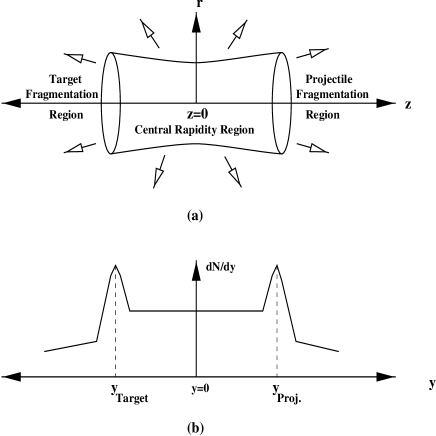
A basic ingredient of the hydrodynamic description of the collision volume is the existence of a strong interaction time scale,
| (4.2) |
In any hadronic collision the produced fragments can only interact after a proper time has elapsed after their collisions. Thus, there is another time scale in the problem, the so called transit time , which is defined as
| (4.3) |
is the nuclear radius, is the Lorentz factor. If the value of (which is a function of the collision energy) is such that then most of the secondaries are formed after the nuclei pass through each other. Consequently these secondaries will not contribute to the energy density of the fluid in the central region (see Fig. (4.1a)). Such a scenario may be realized in the highly relativistic collisions of heavy ions. This particular feature has been taken into account in Bjorken’s hydrodynamic model [29].
It has been observed experimentally that the particle spectra for the secondaries produced in collisions exhibit a central plateau in the rapidity space. This kind of behaviour is due to the frame independence symmetry of the hydrodynamic expansion of the system [28]. Bjorken assumed that the same kind of plateau will also be observed in nucleus-nucleus collisions [29]. In terms of the initial condition this means that the energy density, pressure etc. (all the thermodynamic quantities) will be a function of the initial thermalization (proper) time only and will not depend on the space time rapidity (defined later). This initial symmetry of the thermodynamic quantities is preserved throughout the evolution scenario. If the particle rapidity density is flat or invariant under Lorentz boosts then the entropy density () will be independent of the rapidity.
The evolution of the fluid is governed by the energy-momentum conservation equation
| (4.4) |
where
| (4.5) |
is the energy-momentum tensor for ideal fluid; and are the energy density and pressure of the fluid element. For an isentropic flow the entropy conservation reads
| (4.6) |
where is the entropy current. Considering fluid motion along the (beam) direction, where the fluid rapidity is given by
| (4.7) |
being the fluid velocity. Let us consider the situation in a two dimensional sub-space ( plane). We will make a change of variables from () to () where
| (4.8) |
being the space-time rapidity. As a result Eqs. (4.4) and (4.6) become
| (4.9) |
| (4.10) |
In order to solve these equations we need to know how the fluid velocity depends on the space-time coordinates, i.e. we need as a function of . We will make use of the observation that the amount of particle production is intimately connected with the stopping of the colliding nuclei. At high collision energies the nuclei would slow down considerably, but due to the large rapidity gap between the colliding nuclei, the produced matter will still span a large rapidity interval as seen in Fig. (4.1b). The rapidity distribution of secondaries is likely to exhibit a plateau-like structure in the central region as conjectured by Bjorken. In this situation it is reasonable to assume that in the central rapidity region the longitudinal velocity of produced matter exhibits scaling behaviour,
| (4.11) |
We then have and becomes the proper time of the fluid frame which is related to the centre of mass frame by a Lorentz transformation along the -axis with velocity . Putting in Eqs. (4.9) and (4.10) we get
| (4.12) |
and
| (4.13) |
Equation (4.13) implies that is independent of and so are all the thermodynamic quantities; they depend only on . This gives rise to the frame independence or boost-invariant expansion. From Eq. (4.12) we have
| (4.14) |
which is the Bjorken’s scaling solution. The resulting space-time picture of the collision is shown in Fig. (1.2) of Chapter 1. It may be noted that the above results were obtained without any specific input from the equation of state. It is thus a general result that one dimensional similarity flow is necessarily isentropic even if there is a phase transition. For a relativistic massless gas with statistical degeneracy , and are related through the equation of state:
| (4.15) |
Putting this expression for entropy density in the Bjorken scaling solution we get the cooling law
| (4.16) |
which is routinely used to evaluate the signals of QGP. The initial temperature of the system is determined by observing that the variation of temperature from its initial value to final value (freeze-out temperature) with proper time () is governed by the entropy conservation (Eq. (4.12))
| (4.17) |
The entropy density is then expressed in terms of the observed particle (pion) multiplicity. Using Eqs. (4.15) and (4.17) one gets the initial temperature as
| (4.18) |
where is the total pion multiplicity, is the radius of the system, is the initial thermalization time, and is the Reimann zeta function. is the degeneracy of the produced system and stands for either QGP or a hot hadronic gas. The rapidity density for the secondaries is obtained as [199],
| (4.19) |
where is known as the rescattering parameter. can be parametrized to fit the experimental data in the central region as
| (4.20) |
The assumption of a central plateau in the rapidity distribution is not experimentally observed in nucleus-nucleus collisions at the presently available energies. Hence the boost invariant hydrodynamics may not be a valid concept at these energies. The concept of complete stopping in Landau model [200] is not valid either at these energies. The physical situation may be in-between the boost invariant model of Bjorken and the Landau model of complete stopping, which means that there may be an overlap between the formation zone and the collision zone. However, for its simplicities the Bjorken model will be used to describe the space time evolution of matter formed in URHICs. Appropriate generalization has been made to take into account the temperature dependent hadronic masses in the evolution.
It is worth mentioning that though significant stopping of baryons have been observed in relativistic collisions of heavy ions in the recently concluded experiments at the CERN SPS we will assume the central region in rapidity space to be approximately free of baryons. With strong stopping the net baryon density in the central region can be appreciable but the matter is still not baryon rich because strong stopping also causes large secondary particle production and baryons form only a small fraction of all particles. In other words, the ratio of the baryon chemical potential to the temperature is small. However, at RHIC and LHC the net baryon number can certainly be neglected in the central rapidity region.
4.2 Initial Conditions and Equation of State
The set of hydrodynamic equations is not closed by itself; the number of unknown variables exceeds the number of equations by one. One thus needs to postulate a functional relation between any two variables so that the system becomes deterministic. The most natural course is to look for such a relation between the pressure and the energy density . Under the assumption of local thermal equilibrium, this functional relation between and is the EOS. Obviously, different EOS’s will govern the hydrodynamic flow quite differently [201] and as far as the search for QGP is concerned, the goal is to look for distinctions in the observables due to the different EOS’s (corresponding to the novel state of QGP vis-a-vis that for the usual hadronic matter). It is thus imperative to understand in what respects the two EOS’s differ and how they affect the evolution in space and time. Recently, the sensitivity of the photon emission rate on various evolution scenarios has been studied in Ref. [202].
A physically intuitive way of understanding the role of the EOS in governing the hydrodynamic flow lies in the fact that the velocity of sound sets an intrinsic scale in the hydrodynamic evolution. One can thus write a simple parametric form for the EOS: . For an ideal gas of massless constituents . Inclusion of interactions, however, may drastically alter the value of [203]. In our calculation we assume the MIT bag model equation of state for the QGP where the energy density and pressure are given by
| (4.21) |
and
| (4.22) |
The effective degrees of freedom in QGP, for two flavours. The entropy density is given by . Putting the initial temperature for a system produced as QGP can be determined from Eq. (4.18).
In the hadronic phase we have to be more careful about the presence of heavier particles and the change in their masses due to finite temperature effects. The ideal limit of treating the hot hadronic matter as a gas of pions originated from the expectation that in the framework of local thermalization the system would be dominated by the lowest mass hadrons while the higher mass resonances would be Boltzmann suppressed. Indirect justification of this assumption comes from the experimental observation in high energy collisions that most of the secondaries are pions. Nevertheless, the temperature of the system is higher than during a major part of the evolution and at these temperatures the suppression of the higher mass resonances may not be complete. It may therefore be more realistic to include higher mass resonances in the hadronic sector, their relative abundances being governed by the condition of (assumed) thermodynamic equilibrium. The hadronic phase is taken to consist of , , , , mesons and nucleons. The nucleons and heavier mesons may play an important role in the EOS in a scenario where mass of the hadrons decreases with temperature.
The energy density and pressure for such a system of mesons and nucleons are given by
| (4.23) |
and
| (4.24) |
where the sum is over all the mesons under consideration and stands for nucleons and . The entropy density is then
| (4.25) |
where is the effective statistical degeneracy. Thus, we can visualize the finite mass of the hadrons having an effective degeneracy . Because of the temperature dependence of the effective degeneracy Eq. (4.18) has to be solved self-consistently in order to calculate the initial temperature of the system initially produced as a hot hadronic gas. We thus solve the equation
| (4.26) |
where . The change in the expansion dynamics as well as the value of the initial temperature due to medium effects enters the calculation of the photon emission rate through the effective statistical degeneracy.
If the energy/entropy density in the fireball immediately after the so-called “formation time” is sufficiently high, then the matter exists in the form of a QGP. As the hydrodynamic expansion starts, the system begins to cool until the critical temperature is reached at a time . At this instant, the phase transition to the hadronic matter starts. Assuming that the phase transition is a first order one, the released latent heat maintains the temperature of the system at the critical temperature , even though the system continues to expand; the cooling due to expansion is compensated by the latent heat liberated during the process. Together with the possible explosive events, we are neglecting the scenarios of supercooling or superheating. This process continues until all the matter has converted to the hadronic phase at a time , still at ; from then on, the system continues to expand, governed by the EOS of the hot hadronic matter till the freeze-out temperature is reached at the proper time . Thus the appearance of the so called mixed phase at , when QGP and hadronic matter co-exist, is a direct consequence of the first order phase transition. The possibility of the mixed phase affects the bulk features of the evolution process and plays an important role in QGP diagnostics.
In the mixed phase, the relative proportion of QGP and hadronic matter must be a function of time; initially the system consists entirely of QGP and at the end, entirely of hot hadronic matter. If we denote the fraction of the QGP by then the hadronic fraction in the mixed phase is so that and . Then the entropy density in the mixed phase is given by
| (4.27) |
where () denotes the entropy density of QGP (hadronic) phase at . The life-time of the mixed phase is given by
| (4.28) |
The scaling law governing the variation of with must continue to hold also in the mixed phase; substituting Eq. (4.27) in Eq. (4.12) we obtain for ,
| (4.29) |
where () is the ratio of the degeneracy of QGP phase and the effective degeneracy in the hadronic phase. In the above equation we have used the relation , valid for () dimensional isentropic expansion.
Since the entropy density in any phase can be expressed as in Eq. (4.27) with suitable values of , the volume fractions can also be expressed as
| (4.30) |
If , i.e. if the system is formed in the mixed phase with a fraction of the QGP phase then
| (4.31) |
The mixed phase in this case ends at a proper time . For , the value of is always unity.
Now that we have all the necessary requisites, we will evaluate the photon and dilepton yield in heavy ion collisions at the SPS and RHIC. We will consider two possibilities:
A +A (QGP)(Mixed Phase)Hadronic Phase
or
A + A Hadronic Phase.
The former (latter) case where the initial state is formed in QGP (hadronic) phase will be called the ‘QGP scenario’ (‘no phase transition scenario’). For the QGP sector we use a simple bag model equation of state (EOS) with two flavour degrees of freedom. The temperature in the QGP phase evolves according to Bjorken scaling law . The cooling law in the hadronic sector is quite different from that of the QGP because of the presence of massive hadrons. These hadrons redress themselves in the medium thereby changing their vacuum masses. This is accounted for by introducing temperature dependence in the statistical degeneracy which takes care of the mass varying with temperature. In Table 1 we quote the values of the initial temperatures obtained by assuming various mass variation scenarios. The value of initial thermalization time has been assumed as 1 fm/c both for SPS and RHIC energies. The multiplicity density() in the two cases are given as 600 and 1735 respectively. For a two-flavour QGP the effective degeneracy is 37. The freezeout time is taken as 130 MeV [143] in all the calculations. and dictate the variation of temperature with proper time for the hadronic matter according to the cooling law . The values of indicates a slower cooling in the hadronic phase as compared to that of QGP phase where .
| =600 =1 fm | =1735 =1 fm | ||||||
|---|---|---|---|---|---|---|---|
| hadronic gas | QGP + Mix + Had | QGP + Mix + Had | |||||
| initial state | =185 MeV =1.6 fm | =265 MeV =4.6 fm | |||||
| (MeV) | (fm) | (fm) | |||||
| bare masses | 270 | 10.8 | 0.267 | 0.215 | 31.9 | 0.337 | 0.215 |
| QHD | 220 | 9.4 | 0.247 | 0.194 | 27.6 | 0.305 | 0.194 |
| BR | 195 | 8.2 | 0.236 | 0.184 | 23.9 | 0.288 | 0.185 |
| Nambu | 195 | 4.7 | 0.203 | 0.151 | 13.9 | 0.239 | 0.152 |
Table 1 : Values of initial temperatures and evolution parameters for SPS and RHIC.
In Fig. (4.2) we depict the variation of effective degeneracy as a function of temperature with and without medium effects on the hadronic masses for various scenarios. We observe that for MeV the effective degeneracy becomes larger due to the reduction in temperature dependent masses compared to the free hadronic masses.

Physically this means that the number of hadrons in a thermal bath at a temperature is more when in-medium mass reduction is taken into account. Eq. (4.26) implies that for a given pion multiplicity the initial temperature of the system will be lower (higher) when medium effects on hadronic masses are considered (ignored). This is clearly demonstrated in Fig. (4.3) where we show the variation of temperature with proper time for different initial conditions. The thick dots indicate the yield when QGP is formed initially at MeV and cools down according to Bjorken law up to a temperature at proper time , at which a phase transition takes place; it remains constant at up to a time fm/c after which the temperature decreases as (when medium effects are taken from QHD) to a temperature . If the system is considered to be formed in the hadronic phase then the initial temperature is obtained as MeV (270 MeV) when in-medium effects on the hadronic masses from the QHD model is taken into account (ignored). The corresponding cooling laws are displayed in Fig. (4.3). The above parametrizations of the cooling law in the hadronic phase have been obtained by solving Eq. (4.17) self-consistently. An initial state with the vanishing meson masses at MeV ( fm/c) could be realized in the case of BR and Nambu scaling scenarios with pion multiplicity .

At RHIC a scenario of a pure hot hadronic system within the format of the model used here, appears to be unrealistic. The initial temperature considering bare hadronic masses turns out to be 340 MeV whereas for the other extreme case of massless hadrons it is 290 MeV. With temperature dependent masses the initial temperature will lie somewhere between these two values. For such high temperatures, clearly a hot dense hadronic system cannot be a reality, the hadrons would have melted away even for lower temperatures. Thus, for RHIC we have treated the case of a QGP initial state only. The temperature profile for RHIC is depicted in Fig. (4.4) where we observe that the length of the plateau, which indicates the life time of the mixed phase , depends on the masses of the hadrons in the hadronic phase. The effective degeneracy plays an important role here. At the transition point there is a large decrease in the entropy density. This decrease has to be compensated by the expansion (increasing the volume) to keep the total entropy constant. Since we are considering (1+1) dimensional isentropic expansion, this change in the entropy density will be compensated by increasing which is a measure of the volume, so that the total entropy remains constant. We have seen earlier (Fig. 4.2) that the effective degeneracy in the hadronic phase is the largest for the Nambu scaling and smallest for the bare mass scenario, resulting in smallest (largest) discontinuity in the entropy density for the former (latter) case. Consequently the time taken for the system to compensate the decrease of the entropy density in the Nambu scaling scenario is smaller compared to the case where bare masses are considered. Hence the life time of the mixed phase for the Nambu scaling case is smaller than all other cases.

4.3 Electromagnetic Spectra in URHICs
Our ultimate goal in URHICs is to distinguish between the two possibilities described above, that of a hot hadronic gas initial state or a QGP which undergoes a phase transition to hadronic matter via a mixed phase of coexisting quark and hadronic matter. In the following we will compare the photon and dilepton spectra originating from these two scenarios. As discussed before, the experimentally observed photon and dilepton spectra originating from an expanding QGP or hadronic matter is obtained by convoluting the static (fixed temperature) rate with expansion dynamics. In a first order phase transition scenario the photon and dilepton spectra from a dimensionally expanding system is obtained as
| (4.32) | |||||
where is the radius of the nuclei and functions are introduced to get the contribution from the QGP, mixed and hadronic gas (HG) phases. For (1+1) dimensional expansion, . In the case of photons stands for ; and being the transverse momentum and rapidity of the emitted photon. For dileptons, where, , and are the invariant mass, the transverse momentum and rapidity of the lepton pair respectively.
4.3.1 Photon Spectra at SPS
The thermal photon spectra at SPS energies is shown in Fig. (4.5). In order to interpret the spectra corresponding to the different scenarios let us recall that the effective degeneracy in the hadronic phase is obtained as a function of by solving Eq.(4.25). A smaller (larger) value of is obtained in the free (effective) mass scenario. As a result we get a larger (smaller) initial temperature by solving Eq.(4.26) in the free (dropping) mass scenario for a given multiplicity. Naively we expect that at a given temperature if a meson mass drops its Boltzmann factor will be enhanced and more of those mesons will be produced leading to more photons [105, 204]. However, a larger drop in the hadronic masses results in smaller initial temperature, implying that the space time integrated spectra crucially depends on these two competitive factors. Therefore, with (without) medium effects one integrates an enhanced (depleted) static rate over smaller (larger) temperature range for a fixed freeze-out temperature ( MeV). In the present calculation the enhancement in the photon emission due to the higher initial temperature in the free mass scenario (where static rate is smaller) overwhelms the enhancement of the rate due to negative shift in the vector meson masses (where the initial temperature is smaller). Accordingly, in the case of bare mass ( Nambu scaling) scenario the photon yield is the highest (lowest). In case of the QHD model, the photon yield lies between the above two limits. In the ‘QGP scenario’ the photon yield with in-medium mass is lower than the case where bare masses of hadrons are considered. However, the difference is considerably less than the ‘no phase transition scenario’. This is because, in this case the initial temperature is determined by the quark and gluon degrees of freedom and the only difference between the bare and effective mass scenarios is due to the different lifetimes of the mixed phase. In Fig. (4.5), the photon spectra in the ‘no phase transition scenario’ overshines the ones from the ‘QGP scenario’.


We now compare the above set of curves to the preliminary single photon data obtained by the WA98 Collaboration [205] in Fig. (4.6). We find that for the entire range of the photon spectra in the ‘no phase transition scenario’ with medium effects evaluated in the QHD as well as Nambu scaling scenario explain the data reasonably well. However, the yield with the QHD model parameters seems to overpredict in the low region by a small amount. A QGP initial state as well as a hadronic gas initial state with vacuum properties of hadrons seem to be improbable. The thermal photon spectra for Pb-Pb collisions at SPS have also been evaluated in Ref. [202] for a variety of evolution scenarios without introducing medium effects.
We have also compared the thermal photon spectra evaluated [142] in the QGP and hadronic gas scenarios with the data obtained by the WA80 [206] collaboration. This is shown in Fig. (4.7). The experimental data in this case is the upper bound of the thermal photons in S-Au collisions at 200 A GeV at the CERN SPS. The pion multiplicity is given as 225. Our conclusions are very similar to the Pb-Pb case. The photons evaluated in the hadronic gas scenario with bare masses (short-dashed line) can be ruled out.
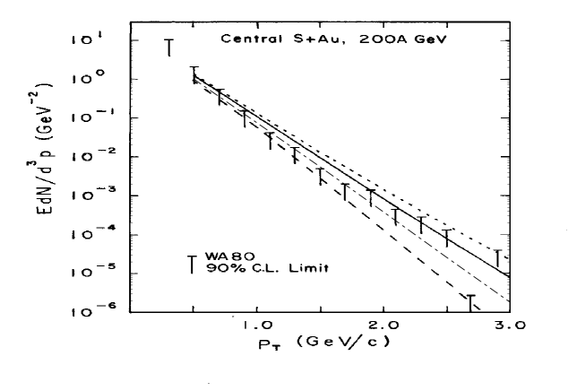
Also, in such a scenario when medium effects from QHD are incorporated, the yield (solid line) just crosses the upper bound. However, thermal photons in the ‘no phase transition scenario’ with medium effects according to Nambu scaling (dot-dashed line) turns out to be a viable description. Quite a few attempts have been made to explain the WA80 upper bound using various models. Using relativistic hadron transport model Li et al [207] have shown that the photon spectra with either free or in-medium meson masses in dense matter do not exceed the upper limit. With in-medium modifications of mesons calculated in the hidden local symmetry approach, Halasz et al [188] have reached similar conclusions. However, using (3+1) dimensional expansion as well as various probable equation of states Sollfrank et al [208] does not claim evidence for a phase transition. The WA80 data have also been explained by Hui et al [209] in a hadron and string cascade model. These results are in sharp contrast to the calculations performed by Srivastava and Sinha [210], Shuryak et al [211, 212], Dumitru et al [213], Arbex et al [214], Neumann et al [215] and Song [204] who have concluded that the WA80 upper limits are satisfied only if a QGP is assumed to have been formed in the initial stages.
4.3.2 Dilepton Spectra at SPS
The space time integrated dilepton spectra for the ‘QGP scenario’ and ‘no phase transition scenario’ with different models of mass variation are shown in Fig. (4.8). The shifts in the invariant mass distribution of the spectra due to the reduction in the hadronic masses, particularly the meson mass, according to the different models are distinctly visible. Their is no appreciable difference between the QGP and ‘no phase transition’ scenarios which is expected because one is looking at low values of the invariant mass where the dominant contribution in either case will be from hadronic matter. Dileptons originating from the high temperature QGP phase will show up at higher values of .
Let us now make a comparison of our predictions with the dielectron spectrum in Pb-Au collisions at 158 A GeV as measured by the CERES Experiment [216]. In this case one has to incorporate [208] the kinematical cuts in the momenta of the electron and the positron relevant for the CERES detector. In Fig. (4.9) we have plotted the dilepton yield normalized to within the rapidity interval 2.1 to 2.65 in the ‘no phase transition scenario’ with the spectral functions in the QHD and Nambu scaling scenarios. We observe that dileptons from an evolving hot hadronic gas with medium modifications calculated in the Nambu scaling scenario clearly fits the data beyond 500 MeV. The QHD model calculations under similar conditions overshoots the data in the region of the shifted peak between 500 and 700 MeV.


Though not a direct signal of QGP, the observed enhancement of low-mass dileptons compared to the yield from hadronic decays at freeze-out (shown by the dotted curve in Fig. (4.9)) has triggered a host of theoretical activity. Though the pion annihilation channel via the meson accounts for a large fraction of this enhancement, it turns out that a quantitative explanation of the data requires the incorporation of medium modifications of the vector mesons. Li, Ko and Brown [143] were the first to achieve an excellent agreement with the CERES data using a decreased mass in the dense fireball. Rapp et al [78] have used a large broadening of the meson line shape and hence a shorter life time due to scattering off baryons in order to explain the data. However, both approaches rely on a high baryon density for the dropping mass or the enlarged width of the meson but the role of baryons is still a debatable issue. It is worth mentioning that we have assumed zero baryon density in our calculations. Koch [217] also finds very little effect due to baryons and are able to obtain a reasonable explanation of the data. It is worth emphasizing here that as yet it has not been possible to explain [208, 218] the observed low-mass enhancements of dileptons measured in the Pb-Au collisions as well as in the S-Au collisions at the CERN SPS in a scenario which does not incorporate medium induced dropping of the vector meson mass, the meson mass in particular [212].
4.3.3 Photon and Dilepton Spectra at RHIC

Finally we study the electromagnetic probes for RHIC energies. As discussed earlier, in this case a scenario of a pure hot hadronic system appears to be unrealistic. So we have treated the case of a QGP initial state only. The baryonic chemical potential has been taken to be zero, which in this case is certainly a valid assumption as far as the central rapidity region is concerned. The thermal photon yield for RHIC is displayed in Fig. (4.10). The solid line represents the total thermal photon yield originating from initial QGP state, mixed phase and the pure hadronic phase. The short dash line indicates photons from quark matter (QM) (= pure QGP phase + QGP part of the mixed phase) and the long dash line represents photons from hadronic matter (HM) (= hadronic part of the mixed phase + pure hadronic phase). In all these cases the effective masses of the hadrons have been taken from Nambu scaling. For GeV photons from QM overshines those from HM since most of these high photons originate from the high temperature QGP phase. The dotted and the dot-dash lines indicate photon yields from QM and HM respectively with bare masses in the hadronic sector. The HM contribution for the bare mass is larger than the effective mass (Nambu) scenario because of the larger value of the life time of the mixed phase in the earlier case (see Table 1). It is important to note that for GeV, the difference in the QM and HM contribution in the effective mass scenario is more that the bare mass scenario.

Thermal dilepton yield at RHIC energies for QGP initial state for different mass variation scenarios are shown in Fig. (4.11). The shape of the peak in the dilepton spectra in case of QHD is slightly different (broader) from the other cases because of the larger mass separation between and mesons in this case (see Fig. (3.16)). The dilepton yield beyond the vector meson peak is larger in the bare mass scenario because of larger initial temperature as seen in Table 1.
Chapter 5 Summary and Discussions
As emphasized in Chapter 1, electromagnetic signals are the only direct probes of evolving strongly interacting systems and hence the study of their spectra is of tremendous importance as far as the detection of QGP in URHICs is concerned. In this thesis we have studied photon and dilepton production from a thermal source composed of strongly interacting matter, QGP or a hot hadronic gas, likely to be produced in the ultra-relativistic collisions of heavy ions.
In Chapter 2 we have reviewed the formulation of photon and lepton pair production from a thermal medium in the framework of Thermal Field Theory. We have seen that the production rate per unit time per unit volume is proportional to the electromagnetic current correlation function or, more generally, to the spectral function of the photon in the medium. Neglecting the possible reinteractions of the virtual photon on its way out of the medium, the emission rate is found to be proportional to the retarded self energy of the photon. In Chapter 2 we have also reviewed how Hard Thermal Loop (HTL) resummation technique has been used to cancel the infra-red divergences so as to obtain finite rates of photon emission due to quark and gluon interactions in the QGP.
As mentioned in the introduction, our main emphasis has been to study the effect of the medium modifications of hadronic properties, particularly of the and mesons, on the spectra of photons and dileptons obtained in URHICs. In Chapter 3 we have made a detailed study of the static (fixed temperature) rates of photon and dilepton emission from hadronic matter incorporating medium modifications of the masses and decay widths of vector mesons evaluated within various well-known models. In the Quantum Hadrodynamic (QHD) model the and masses are found to decrease differently. The disentanglement of the and peaks in the dilepton spectrum resulting from URHICs would be an excellent evidence of in-medium mass shift of vector mesons [194] and/or the validity of such model calculations for the situation under consideration. We have studied the modification of the spectral functions of the and mesons using QCD sum rules at finite temperature. Here, the hadronic spectral function in vacuum have been parametrized using the experimental data on in terms of a resonance and a continuum. Due to the lack of our understanding of the critical behaviour of scalar and tensor condensates the vector meson masses and continuum threshold as a function of temperature were taken to vary according to Brown-Rho and Nambu scaling. The interesting possibility of the disappearance of the and peaks in the dilepton spectra due to temperature induced lowering of the continuum threshold was investigated. We have also made a brief study of the mass modifications within the gauged linear and non-linear sigma models and the hidden local symmetry approach. The changes in these models are observed to be small. The static rates of photon and dilepton production from interacting hadronic matter have been evaluated. It is observed that the in-medium effects on the dilepton and the photon spectra are prominently visible for QHD model and Brown-Rho and Nambu scaling scenarios. It is interesting to note that the dilepton spectra spectra is affected by both the changes in the decay width as well as in the mass of the vector mesons whereas the photon spectra is affected only by the change in the mass of the vector mesons and is rather insensitive to the change in width. The effects of the continuum on the dilepton spectra are seen to be substantial.
In Chapter 4 the photon and dilepton yield from a longitudinally expanding system likely to be produced in URHICs at the SPS was contrasted between a QGP initial state and a hot hadronic gas initial state scenarios. It was observed that the incorporation of medium modifications resulted in substantial changes in the evaluation of the initial temperature as well as the cooling profile. When compared with the preliminary Pb-Pb data obtained by the WA98 Collaboration we find that the photon yield in the hot hadronic gas scenario with medium effects calculated from QHD as well as Nambu scaling scenarios explain the data reasonably well. Similar conclusions were reached when we compared the thermal photon yield in S-Au collisions at 200 AGeV to the upper limits obtained by the WA80 Collaboration. The thermal photon spectra from a hadronic gas with spectral modifications evaluated in the Nambu scaling scenario falls within the experimental upper limits. The corresponding QHD model calculations does not seem to qualify as a viable possibility in this case.
We have also compared the results of the dielectron yield to the Pb-Au data obtained by the CERES Collaboration. Here again the hot hadronic gas scenario with medium effects in the Nambu scaling scenario seem to fit the data fairly well. This is certainly due to the increased production of low mass electron pairs originating mainly from the decay of mesons with decreased mass and enhanced width in the medium. This is however not a direct signal of QGP because the contribution from the QGP phase is very small in the low invariant mass region.
It is interesting to note that so far the observed low mass enhancement in the dilepton data could not be explained without the consideration of mesons with a depleted mass. In this connection it is worth mentioning that CERES is planning to substantially improve the mass resolution to values of the order of the natural line width of the meson (8.5 MeV). It should then be possible to directly measure the yield of the vector mesons , and even (=4.5 MeV) including any possible changes in their mass or decay width [195]. Also, the mass shifts of vector mesons at zero temperature but finite baryon density could be detected by HADES [196] and CEBAF [64].
In the following we will discuss some general aspects regarding photon and dilepton emission from evolving matter with reference to the calculations presented in this thesis:
The photon production from QGP has been evaluated using HTL resummation based on the assumption , which is impossible to meet in URHICs even at the highest energy to be available at the CERN LHC in future. The strong coupling constant is likely to attain a value 2 at RHIC/LHC. Evaluation of the photon emission rates at such high values of the strong coupling is a formidable task. In this respect the development of methods suitable for addressing non-perturbative effects near and above the QCD phase transition point is of paramount importance. Extension of the self-consistent resummation scheme developed in theory [219] to non-abelian gauge theory [220, 221] would be a very important step towards the understanding of the phenomena near the QCD phase transition.
The exact value of the critical temperature () for deconfinement phase transition is still uncertain. However, recent lattice simulation [13] for two flavour QCD indicates a value of for chiral transition MeV. We have taken MeV, although it is not known whether the values of for the chiral and deconfinement transition are the same or not. The value of the initial thermalization time is unfortunately also an unknown quantity. We take fm/c as a canonical value following Bjorken [29]. A similar value of has been considered in the literature [51, 204, 208]. The freeze-out temperature is another parameter which is not precisely known. This is important because the yield from the hadronic phase depends substantially on the value of . We have also considered a baryon-free system based on the assumption that the ratio of the baryon chemical potential to the temperature is reasonably small. This might not be totally justified at SPS energies, but at RHIC a baryon-free central region is certainly a possibility.
We have assumed thermodynamic equilibrium in our calculations. Such a situation may not be realized practically [31, 32, 222, 223, 224, 225]. Also, emissions from the pre-equilibrium era may pollute the kinematical domains where one looks for signals of QGP [32]. Unfortunately, although considerable progress has been made [226, 227, 228], the general techniques for solving non-equilibrium quantum field theoretical problems is still in the early stages of development [229].
We have assumed that the produced system behaves as an ideal, non-dissipative fluid. Incorporation of viscosity breaks the time-reversality of the evolution. The ensuing generation of entropy during the temporal evolution invalidates the role of as a handy constant of motion and consequently affects the estimation of the initial temperature [230].
In this thesis we have neglected transverse expansion of the evolving matter. Incorporation of medium modifications in a 3+1 dimensionally expanding system is a non-trivial task. We intend to take up this project in the near future.
We conclude with a few comments based on the experimental results from URHICs at the CERN SPS. From the measured hadron yields and momentum spectra including transverse and directed flow effects there is a strong evidence of production of a collectively behaving strongly interacting matter with a large volume and finite lifetime. The thermal photon spectra as well as the pattern of low-mass enhancement of pairs observed in S-Au, Pb-Pb and Pb-Au collisions also lend support to the picture of a collective thermal system of hadrons. On the other hand, the observation of a significant enhancement in multistrange baryon production as well as the anomalous suppression of in Pb-Pb collisions cannot be explained without invoking partonic degrees of freedom and deconfined matter. At this critical and interesting juncture we look forward to the experiments at RHIC where larger and hotter systems are likely to be produced. Along with quantitative gains in all the signals there is a distinct possibility of direct detection of electromagnetic radiation from the QGP phase which will pave the way for an unambiguous conclusion regarding the formation of this novel form of matter.
Appendix
Invariant Amplitudes for Photon Production
We list the invariant amplitudes for photon production from hadronic matter consisting of , , , and mesons which have been considered in the evaluation of the photon yield from hot hadronic matter. The medium modifications of the and mesons have been taken into account in the respective propagators.
(1)

| (A.1) |
| (A.2) |
(2)
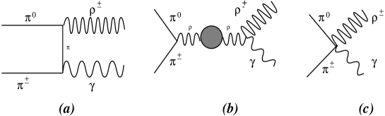
| (A.3) |
| (A.4) |
(3)

| (A.5) |
| (A.6) |
(4)
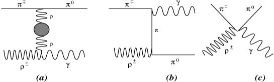
| (A.7) |
| (A.8) |
(5)
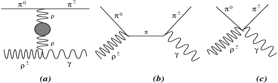
| (A.9) |
| (A.10) |
(6)

| (A.11) |
(7)
| (A.12) |
The coupling constant is evaluated from the following relations:
and keV.
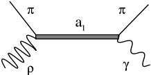
(8)
| (A.13) |
where
and
=5.04 (from decay)
=-0.12, , GeV, GeV, (from decay)
(9) ,
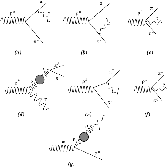
| (A.14) |
| (A.15) |
| (A.16) |
| (A.17) |
| (A.18) |
Bibliography
- [1] D. Gross and F. Wilczek, Phys. Rev. Lett. 30 (1973) 1343; Phys. Rev D8 (1973) 3633.
- [2] H. D. Politzer, Phys. Rev. Lett. 30 (1973) 1346.
- [3] G. t’ Hooft, Under the Spell of Gauge Theory, (Advanced Series in Mathematical Physics, Vol. 19), World Scientific, 1984.
- [4] G. t’ Hooft, Nucl. Phys. B138 (1978) 1; Nucl. Phys. B190 (1981) 455.
- [5] K. G. Wilson, Phys. Rev. D10 (1974) 2445.
- [6] R. Dashen, Phys. Rev. 183 (1969) 1291.
- [7] J. C. Collins and M. J. Perry, Phys. Rev. Lett. 34 (1975) 1353.
- [8] M. Kisslinger and P. Morley, Phys. Rev. D10 (1976) 2765, 2771.
- [9] E. V. Shuryak, Phys. Rep. 61 (1980) 71; Phys. Rep. 115 (1984) 151.
- [10] H. Satz, Ann. Rev. Nucl. Part. Sc. 35 (1985) 245.
- [11] L. McLerran, Rev. Mod. Phys. 58 (1986) 1021.
- [12] J. B. Kogut, Phys. Rep. 67 (1980) 67.
- [13] A. Ukawa, Nucl. Phys. A638 (1998) 339c.
- [14] D. Bailin and A. Love, Nucl. Phys. B205(1982) 119; Phys. Rep. 107 (1984) 325.
- [15] M. Iwasaki and T. Iwado, Phys. Lett. B350 (1995) 163; Prog. Theor. Phys. 94 (1995)1073; M. Iwasaki, Prog. Theor. Phys. 96 (1996)1043; ibid. 98 (1998) 461; ibid. 101 (1999) 19.
- [16] M. Alford, K. Rajagopal and F. Wilczek, Phys. Lett. B422 (1998) 247; R. Rapp, T. Schafer, E. V. Shuryak and M. Velovsky, Phys. Rev. Lett. 81 (1998) 53; N. Evans, S. D. H. Hsu and M. Schwetz, Phys. Lett. B449 (1999) 281; D. T. Son, Phys. Rev. D59 (1999) 094019.
- [17] S. Bonometto and O. Pantano, Phys. Rep. 228 (1993) 175.
- [18] E. Witten, Phys. Rev. D30 (1984) 272.
- [19] A. Bhattacharyya, J. Alam, S. Sarkar, P. Roy, B. Sinha, S. Raha and P. Bhattacharjee, Proc. Quark Matter ’99; Nucl. Phys A661 (1999) 629c; Phys. Rev. D (in press).
- [20] B. Müller, The Physics of Quark Gluon Plasma, Springer, Heidelberg, 1985.
- [21] R. C. Hwa (Ed.), Quark Gluon Plasma 1 and 2, World Scientific, Singapore, 1990, 1995.
- [22] C. Y. Wong, Introduction to High Energy Heavy Ion Collisions, World Scientific, Singapore, 1994.
- [23] K. Werner, Phys. Rep. 232 (1993) 87.
- [24] B. Anderson, G. Gustafsson and B. Nilsson-Almquist, Nucl. Phys. B181 (1987) 289.
- [25] M. Sorge, H. Stöcker, and W. Greiner, Nucl. Phys. A498 (1989) 567c; Ann. Phys. 192 (1989) 266.
- [26] K. Geiger, Phys. Rep. 258 (1995) 237.
- [27] H. von Gersdorff, L. McLerran, M. Kataja, and P. V. Ruuskanen, Phys. Rev. D34 (1986) 794; M. Kataja, P. V. Ruuskanen, L. McLerran, and H. von Gersdorff, Phys. Rev. D34 (1986) 3755.
- [28] C. B. Chiu, E. C. G. Sudarshan and K. H. Wang, Phys. Rev. D12, (1975) 902.
- [29] J. D. Bjorken, Phys. Rev. D27, (1983) 140.
- [30] S. Sarkar, D. K. Srivastava and B. Sinha, Phys. Rev. D51 (1995) 318.
- [31] J. Alam, P. Roy, S. Sarkar, S. Raha and B. Sinha, Int. J. Mod. Phys. A12 (1997) 5151.
- [32] P. Roy, J. Alam, S. Sarkar, B. Sinha and S. Raha, Nucl. Phys. A 624 (1997) 687.
- [33] L. van Hove, Phys. Lett. B118 (1982) 138; Z. Phys, C21 (1983) 93.
- [34] J.-Y. Ollitrault, Proc. Quark Matter ’97; Nucl. Phys. A638 (1998) 195c.
- [35] U. Heinz, Proc. Quark Matter ’96; Nucl. Phys. A610 (1996) 264c.
- [36] S. Pratt, Proc. Quark Matter ’97; Nucl. Phys. A638 (1998) 125c.
- [37] J. Rafelski and B. Müller, Phys. Rev. Lett. 48 (1982) 1066; (1986) 2334(E).
- [38] G. J. Odyniec, Proc. Quark Matter ’97; Nucl. Phys. A638 (1998) 135c.
- [39] F. Antinori et al, Proc. Quark Matter ’99; Nucl. Phys. A661 (1999) 130c.
- [40] A. A. Anselm and M. G. Ryskin, Phys. Lett. B266 (1989) 482.
- [41] R. D. Pisarski, Phys. Lett. B 110 (1982) 155.
- [42] R. D. Pisarski, hep-ph/9503330.
- [43] T. Hatsuda and T. Kunihiro, Phys. Rev. Lett. 55 (1985) 158.
- [44] T. Hatsuda and T. Kunihiro, Phys. Lett. 185B, (1987) 304.
- [45] T. Hatsuda and T. Kunihiro, Phys. Rep. 247 (1994) 221.
- [46] T. Matsui and H. Satz, Phys. Lett B178 (1986) 416.
- [47] J.-P. Blaizot, Proc. Quark Matter ’97; Nucl. Phys. A638 (1998) 373c.
- [48] M. H. Thoma and M. Gyulassy, Nucl. Phys. B351 (1991) 491; E. Braaten and M. H. Thoma, Phys. Rev. D44 (1991) R2625.
- [49] J. D. Bjorken, Fermilab preprint 82/59 -THY.
- [50] L. McLerran and T. Toimela, Phys. Rev. D31 (1985) 545.
- [51] J. Alam, S. Raha and B. Sinha, Phys. Rep. 273 (1996) 243.
- [52] W. Cassing and E. L. Bratkovskaya, Phys. Rep. 308 (1999) 65.
- [53] P. V. Ruuskanen, Nucl. Phys. A 544 (1992) 169c.
- [54] J. I. Kapusta, Nucl. Phys. A 566 (1994) 45c.
- [55] J. I. Kapusta, P. Lichard, and D. Seibert, Phys. Rev. D44 (1991) 2774.
- [56] R. Baier, H. Nakkagawa, A. Niegawa and K. Redlich, Z. Phys. C53 (1992) 433.
- [57] P. Aurenche, F. Gelis, H. Zaraket and R. Kobes, Phys. Rev. D 58 (1998) 085003.
- [58] E. Braaten and R. Pisarski, Nucl. Phys. B 337 (1990) 569; Nucl. Phys. B339 (1990) 310.
- [59] J. Frenkel and J. C. Taylor, Nucl. Phys. B334 (1990) 199.
- [60] P. V. Ruuskanen, Lecture Notes (unpublished).
- [61] U. Meissner, Phys. Rep. 161 (1988) 213.
- [62] M. A. Nowak, M. Rho and I. Zahed, Chiral Nuclear Dynamics, World Scientific, Singapore, 1996.
- [63] B. R. Holstein, Com. Nucl. Part. Phys. 19 (1990) 221.
- [64] J. D. Walecka, Theoretical Nuclear and Subnuclear Physics, Oxford University Press, NY, 1995.
- [65] G. E. Brown and M. Rho, Phys. Rev. Lett. 66 (1991) 2720.
- [66] R. D. Pisarski, Phys. Rev. D 52 (1995) R3773; Nucl. Phys. A 590 (1995) 553c.
- [67] C. Song, Phys. Rev. D 53 (1996) 3962.
- [68] M. Harada and A. Shibata, Phys. Rev. D 55 (1997) 6716.
- [69] E. Shuryak and V. Thorsson, Nucl. Phys. A 536 (1992) 739.
- [70] V. L. Eletsky, B. L. Ioffe and J. I. Kapusta, Nucl. Phys. A 642 (1998) 155c.
- [71] B. D. Serot and J. D. Walecka, Advances in Nuclear Physics Vol. 16, Plenum Press, New York 1986.
- [72] S. A. Chin, Ann. Phys. 108 (1977) 301.
- [73] C. Song, P. W. Xia and C. M. Ko, Phys. Rev. C52 (1995) 408.
- [74] T. Hatsuda, Nucl. Phys. A544 (1992) 27c.
- [75] E. Shuryak, Rev. Mod. Phys. 65 (1993) 1.
- [76] M. A. Shifman, Prog. Th. Phys. (Suppl.) 131 (1998)1; hep-ph/9802214.
- [77] G. E. Brown and M. Rho, Phys. Rep. 269 (1996) 333.
- [78] R. Rapp, G. Canfray and J. Wambach, Nucl. Phys. A 617 (1997) 472; Phys. Rev. Lett. 76 (1996) 368.
- [79] F. Klingl, N. Kaiser and W. Weise, Nucl. Phys. A624 (1997) 527.
- [80] E. L. Feinberg, Nuovo Cim. 34A (1976) 39.
- [81] P. V. Ruuskanen in Particle Production in Highly Excited Matter, Eds. H. H. Gutbrod and J. Rafelski, (Plenum Press, New York, 1993)
- [82] M. Le Bellac, Thermal Field Theory, Cambridge University Press, 1996.
- [83] H. A. Weldon, Phys. Rev. D42 (1990) 2384.
- [84] A. Das, Finite Temperature Field Theory, World Scientific, Singapore, 1997.
- [85] J. I. Kapusta, Finite Temperature Field Theory, Cambridge University Press, 1993.
- [86] N. P. Landsman and Ch. G. van Weert, Phys. Rep. 145 (1987) 141.
- [87] J. F. Nieves, Phys. Rev. D 42 (1990) 4123.
- [88] P. V. Landshoff, hep-ph/9808362.
- [89] R. Kubo, J. Phys. Soc. Japan, 12 (1957) 570; P. Martin and J. Schwinger, Phys. Rev. 115 (1959) 1342.
- [90] M. H. Thoma, hep-ph/9503400.
- [91] H. Weldon, Phys. Rev. D26 (1982) 1394.
- [92] P. Aurenche and T. Becharrawy, Nucl. Phys. B379 (1992) 259.
- [93] A. A. Abrikosov, L. P. Gorkov and I. E. Dzyaloshinski, Sov. Phys. JETP 9 (1959) 636.
- [94] E. S. Fradkin, Sov. Phys. JETP 9 (1959) 912.
- [95] R. D. Pisarski, Nucl. Phys. B309 (1988) 476.
- [96] H. A. Weldon, Phys. Rev. D 28 (1983) 2007.
- [97] L. Dolan and R. Jackiw, Phys. Rev. D9 (1974) 3320.
- [98] L. S. Brown, Quantum Field Theory, Cambridge University Press, 1995.
- [99] H. A. Weldon, Phys. Rev. Lett. 66 (1991) 293.
- [100] V. B. Berestetskii, E. M. Lifshitz and L. P. Pitaevskii, Quantum Electrodynamics, Pergamon Press, 1982.
- [101] C. Gale and J. I. Kapusta, Nucl. Phys. B357, (1991) 65.
- [102] R. Kobes and G. Semenoff, Nucl Phys. B260 (1985) 714; B272, (1986) 329.
- [103] F. Gelis, Nucl. Phys. B508, (1997) 483.
- [104] C. Gale and J. I. Kapusta, Phys. Rev. C35, (1987) 2107.
- [105] S. Sarkar, J. Alam, P. Roy, A. K. Dutt-Mazumder, B. Dutta-Roy, B. Sinha, Nucl. Phys. A634, (1998) 206.
- [106] F. Karsch, Z. Phys. C38 (1988) 147.
- [107] R. Kobes, hep-ph/9511208.
- [108] R. D. Pisarski Nucl. Phys. A525 (1991) 175.
- [109] D. J. Gross, R. D. Pisarski and L. G. Yaffe, Rev. Mod. Phys. 53 (1981) 43.
- [110] V. P. Nair, hep-th/9809086.
- [111] J. P. Blaizot and E. Iancu, hep-ph/9903389.
- [112] A. V. Smilga, hep-ph/9604367.
- [113] A. Linde, Phys. Lett. B 96 (1980)289.
- [114] P. Aurenche, F. Gelis and H. Zaraket, hep-ph/9911367.
- [115] J. C. Taylor and S. M. Wong, Nucl. Phys. B 355 (1990) 115.
- [116] E. Braaten and R. D. Pisarski, Phys. Rev. D 45 (1992) R1827.
- [117] R. Efraty and V. P. Nair, Phys. Rev. Lett. 68 (1992) 2891.
- [118] V. P. Nair, Phys. Rev. D 50 (1994) 4201.
- [119] F. Flechsig and A. K. Rebhan, Nucl. Phys. B464 (1996) 279.
- [120] J. P. Blaizot and E. Iancu, Phys. Rev. Lett. 70 (1993) 3376.
- [121] P. F. Kelly, Q. Liu, C. Lucchesi and C. Manuel, Phys. Rev. Lett. 72 (1994) 3461.
- [122] V. P. Nair, Phys. Rev. D 48 (1993) R3432.
- [123] P. Aurenche, F. Gelis, H. Zaraket and R. Kobes, hep-ph/9903307.
- [124] V. V. Klimov, Sov. J. Nucl. Phys. 33 (1981) 934.
- [125] H. A. Weldon, Phys. Rev. D 26 (1981) 2789; Phys. Rev. D 40 (1989) 2410.
- [126] R. Baier, S. Peigne and D. Schiff, Z. Phys. C62 (1994) 337.
- [127] P. Aurenche, F. Gelis, R. Kobes and E. Petitgirard, Phys. Rev. D54 (1996) 5274.
- [128] T. Kinoshita, J. Math. Phys. 3 (1962) 650.
- [129] T. D. Lee and M. Nauenberg, Phys. Rev. 133 (1964) 1549.
- [130] A. Niegawa, Mod. Phys. Lett. A 10 (1995) 379.
- [131] A. Niegawa, Phys. Rev. Lett. 71 (1993) 3055.
- [132] R Baier, hep-ph/9311343.
- [133] J. M. Cornwall and W. S. Hou, Phys. Lett. B 153 (1985) 173.
- [134] P. Roy, D. Pal, S. Sarkar, D. K. Srivastava and B. Sinha, Phys. Rev. D 53 (1996) 2364.
- [135] L. Landau and I. Pomeranchuk, Dokl. Acad. Nauk. SSSR 92 (1953) 535; ibid 735; A. B. Migdal, Phys. Rev. 103 (1956) 429.
- [136] J. F. Owens, Rev. Mod. Phys. 59 (1987) 465; R. C. Hwa and K. Kajantie, Phys. Rev. D32 (1985) 1109; B. Combridge and C. Maxwell, Nucl. Phys. B239 (1984) 429; R. Gandhi, F. Halzen and F. Herzog, Phys. Lett. 152B (1985) 261..
- [137] A. D. Martin, R. G. Roberts and W. J. Stirling, Phys. Lett. B 306 (1993) 147; 309 (1993) 492 (E).
- [138] T. Altherr and P. V. Ruuskanen, Nucl. Phys. B380 (1992) 377.
- [139] D. Pal, P. Roy, S. Sarkar, D. K. Srivastava and B. Sinha, Phys. Rev. D 55 (1997) 1467.
- [140] S. Sarkar, D. K. Srivastava, B. Sinha, P. Roy, S. Chattopadhyay and D. Pal, Phys. Lett. B 402 (1997) 13.
- [141] V. L. Eletsky and B. L. Ioffe, Phys. Rev. Lett. 78 (1997) 1010.
- [142] S. Sarkar, P. Roy, J. Alam and B. Sinha, Phys. Rev. C60 (1999) 054907.
- [143] G. Q. Li, C. M. Ko and G. E. Brown, Nucl. Phys. A606 (1996) 568.
- [144] H. C. Jean, J. Piekarewicz and A. G. Williams, Phys. Rev. C49, (1994) 1981.
- [145] J. C. Caillon and J. Labarsouque, Phys. Lett. B311 (1993) 19.
- [146] H. Shiomi and T. Hatsuda, Phys. Lett. B334 (1994) 281.
- [147] T. Hatsuda, H. Shiomi and H. Kuwabara, Prog. Th. Phys. 95 (1996) 1009.
- [148] J. Alam, S. Sarkar, P. Roy, B. Dutta-Roy and B. Sinha, Phys. Rev. C 59 (1999) 905.
- [149] S. Weinberg, Phys. Rev. Lett. 18 (1967) 507.
- [150] M. Asakawa, C. M. Ko, P. Levai and X. J. Qiu Phys. Rev. C46 (1992) R1159.
- [151] M. Herrmann, B. L. Friman and W. Nörenberg, Nucl. Phys. A560 (1993) 411.
- [152] G. Chanfray and P. Shuck, Nucl. Phys. A555 (1993) 329.
- [153] B. Friman and H. J. Pirner, Nucl. Phys. A617 (1997) 496.
- [154] R. Rapp, M. Urban, M. Bubballa and J. Wambach, Phys. Lett. B417 (1998) 1.
- [155] W. Peters, M. Post, H. Lenske, S. Leupold and U. Mosel, Nucl. Phys. A632 (1998) 109.
- [156] G. E. Brown, G. Q. Li, R. Rapp, M. Rho and J. Wambach, Acta Phys. Polon. B29 (1998) 2309.
- [157] P. Roy, S. Sarkar, J. Alam, B. Dutta-Roy and B. Sinha, Phys. Rev. C 59 (1999) 2778.
- [158] M. Gell-Mann, D. Sharp and W. D. Wagner, Phys. Rev. Lett. 8 (1962) 261.
- [159] K. Rajagopal and F. Wilczek, Nucl. Phys. B 399 (1993) 395; Nucl. Phys. B 404 (1993) 577.
- [160] S. Gasiorwicz and D. A. Geffen, Rev. Mod. Phys. 41, (1969) 531.
- [161] N. Kroll, T. D. Lee and B. Zumino, Phys. Rev. 157 (1967) 1376.
- [162] J. J. Sakurai, Currents and Mesons, The University of Chicago Press, Chicago, 1969.
- [163] C. N. Yang and R. L. Mills, Phys. Rev. 96 (1954) 191.
- [164] K. Kawarabayashi and M. Suzuki, Phys. Rev. Lett. 16 (1966) 255.
- [165] Riazzuddin and Fayazuddin, Phys. Rev. 147 (1967) 1071.
- [166] R. D. Pisarski, hep-ph/9505257.
- [167] H. Georgi, Nucl. Phys. B 331 (1990) 311.
- [168] C. Song, Phys. Rev. D 48 (1993) 1375.
- [169] B. R. Holstein, Phys. Rev. D 33 (1986) 3316.
- [170] M. Bando, T. Kugo, S. Uehara, K. Yamawaki and Y. Yanagida, Phys. Rev. Lett. 54 (1985) 1215.
- [171] M. Bando, T. Kugo and K. Yamawaki, Phys. Rep. 164 (1988) 217.
- [172] T. Fujiwara, T. Kugo, H. Terao, S. Uehara and K. Yamawaki, Prog. Th. Phys. 73 (1985) 926.
- [173] L. J. Reinders, H. Rubinstein and S. Yazaki, Phys. Rep. 127 (1985) 1.
- [174] B. L. Ioffe, Acta Phys. Polon. B16 (1985) 543.
- [175] M. Shifman (Ed.), Vacuum Structure and QCD Sum Rules, North Holland, Amsterdam, 1992.
- [176] S. Narison, QCD Spectral Sum Rules, World Scientific, Singapore, 1989.
- [177] M. Shifman, A. Vainshtein and V. Zakharov, Nucl. Phys. B147 (1979) 385.
- [178] A. I. Bochkarev and M. E. Shaposhnikov, Nucl, Phys. B268 (1986) 220.
- [179] T. Hatsuda and S. H. Lee, Phys. Rev. C46 (1992) R34.
- [180] T. Hatsuda, Y. Koike and S. H. Lee, Nucl. Phys. B394 (1993) 221.
- [181] N. V. Krasnikov, A. A. Pivovarov and N. N. Tavkhelidze, Z. Phys. C19 (1983) 301.
- [182] J. I. Kapusta and E. Shuryak, Phys. Rev. D49 (1994) 4694.
- [183] S. H. Lee, Phys. Rev. C 57 (1998) 927; hep-ph/9904007.
- [184] M. Dey, V. L. Eletsky and B. L. Ioffe, Phys. Lett. B252 (1990) 620.
- [185] P. Roy, S. Sarkar, J. Alam and B. Sinha, Nucl. Phys. A 653 (1999) 277.
- [186] L. Xiong, E. V. Shuryak and G. E. Brown, Phys. Rev. D46 (1992) 3798.
- [187] C. Song, Phys. Rev.C47 (1993) 2861.
- [188] M. A. Halasz, J. V. Steel, G. Q. Li and G. E. Brown, Phys. Rev. C 58 (1998) 365.
- [189] J. K. Kim, P. Ko, K. Y. Lee and S. Rudaz, Phys. Rev. D53 (1996) 4787.
- [190] P. Ko and S. Rudaz, Phys. Rev. D 50 (1994) 6877.
- [191] V. L. Eletsky and J. I. Kapusta, Phys. Rev. C 59 (1999) 2757.
- [192] R. N. Cahn, Phys. Rev. D7 (1973) 247.
- [193] H. A. Weldon, Ann. Phys. 228 (1993) 43.
- [194] I. Ravinovich, Nucl. Phys. A638 (1998) 159c.
- [195] I. Tserruya, nucl-ex/9912003.
- [196] http://piggy.physik.uni-giessen.de/hades/
- [197] E. V. Shuryak, hep-ph/9906443.
- [198] R. Rapp, hep-ph/9907342.
- [199] U. Heinz, P. Koch and B. Friman, Proc. Large Hadron Collider Workshop, Aachen (1990), CERN-90-10, Vol. II, p.1079.
- [200] D. ter Haar (Ed.), Collected papers of L. D. Landau, Gordon and Breach, London, 1965.
- [201] P. Huovinen, P. V. Ruuskanen and J. Sollfrank, Nucl. Phys. A650 (1999) 227.
- [202] D. Yu. Peressounko and Yu. E. Pokrovsky, hep-ph/9906325.
- [203] M. Asakawa and T. Hatsuda, Phys. Rev. D55 (1998) 4488.
- [204] C. Song and G. Fai, Phys. Rev. C58 (1998) 1689.
- [205] WA98 collaboration, private communication.
- [206] R. Albrecht et al Phys. Rev. Lett. 76 (1996) 3506.
- [207] G. Q. Li, G. E. Brown, C. Gale, and C. M. Ko, nucl-th/9712048.
- [208] J. Sollfrank, P. Huovinen, M. Kataja, P. V. Ruuskanen, M. Prakash and R. Venugopalan, Phys. Rev. C55 (1997) 392.
- [209] W. Hui, S. Ben-Hao, T. An, and S. Zu-Xun, nucl-th/9904035.
- [210] D. K. Srivastava and B. Sinha, Phys. Rev. Lett. 73 (1994) 2421.
- [211] E. V. Shuryak and L. Xiong, Phys. Lett. B333 (1994) 316.
- [212] C. M. Hung and E. V. Shuryak, Phys. Rev. C56 (1997) 453.
- [213] A. Dumitru, U Katscher, J. A. Mahrun, H. Stöcker, W. Greiner, and D. H. Rischke, Phys. Rev. C51 (1995) 2166.
- [214] N. Arbex, U. Ornik, M. Plumer, A. Timmermann, and R. Weiner, Phys. Lett. B345 (1995) 307.
- [215] J. J. Neumann, D. Siebert and G. Fai, Phys. Rev. C51 (1995) 1460.
- [216] B. Lenkeit, Proc. Quark Matter ’99; Nucl. Phys. A661 (1999) 23c.
- [217] V. Koch, nucl-th/9903008; V. Koch and C. Song, Phys. Rev C54 (1996) 1903.
- [218] D. K. Srivastava, B. Sinha, and C. Gale, Phys. Rev. C53 (1996) R567.
- [219] S. Chiku and T. Hatsuda, Phys. Rev. D 57 (1998) R6; Phys. Rev. D 58 (1998) 076001.
- [220] J. O. Anderson, E Braaten and M. Strickland, hep-ph/9905337.
- [221] J. P. Blaizot, E. Iancu and A. Rebhan, hep-ph/9906340.
- [222] K. Geiger, Phys. Rep. 258 (1995) 237.
- [223] X. N. Wang, , Phys. Rep. 280 (1997) 287.
- [224] J. Alam, S. Raha and B. Sinha, Phys. Rev. Lett. 73, (1994) 1895.
- [225] H. Sorge, H. Stöcker and W. Greiner, Nucl. Phys. A 498 (1989) 567c.
- [226] A. Niegawa, Prog. Theor. Phys. 102 (1999) 1.
- [227] M. Thoma, hep-ph/9808359.
- [228] M. Burgess, hep-ph/9808116.
- [229] K. Kajantie, Nucl. Phys. A 610 (1996) 26c.
- [230] S. Sarkar, P. Roy, J. Alam, S. Raha and B. Sinha, J. Phys. G23 (1997) 469.