Nucleon Properties in the Covariant
Quark-Diquark Model

Abstract

In the covariant quark-diquark model the effective Bethe-Salpeter (BS) equations for the nucleon and the $\Delta$ are solved including scalar and axialvector diquark correlations. Their quark substructure is effectively taken into account in both, the interaction kernel of the BS equations and the currents employed to calculate nucleon observables. Electromagnetic current conservation is maintained. The electric form factors of proton and neutron match the data. Their magnetic moments improve considerably by including axialvector diquarks and photon induced scalar-axialvector transitions. The isoscalar magnetic moment can be reproduced, the isovector contribution is about 15% too small. The ratio $\mu\,G_{E}/G_{M}$ and the axial and strong couplings $g_{A}$, $g_{\pi NN}$, provide an upper bound on the relative importance of axialvector diquarks confirming that scalar diquarks nevertheless describe the dominant 2-quark correlations inside nucleons.

1 Introduction

High-precision data on nucleon properties in the medium-energy range are available by now or will be in near future. This is especially the case for their electromagnetic form factors. From a theoretical point of view the behavior of the form factors indicates the necessity of a relativistic description of the nucleon. Non-relativistic constituent models generally fail beyond a momentum transfer of a few hundred MeV.

From relativistic quantum mechanics of three constituent quarks models employing effective Hamiltonian descriptions were deduced. However, the necessity for the effective Hamiltonian to comply with the Poincaré algebra and, at the same time, with the covariance properties of the wave functions leads to fairly complicated constraints to ensure the covariance of current operators Leu78 . While some phenomenological studies relax these constraints and allow for covariance violations of one-body currents Szc95 , others put emphasis on the consistent transformation of those components of one-body currents that are relevant in light-front Hamiltonian dynamics Chu91 ; Kap95 ; Sal95 . The inclusion of two-body currents was considered within a semi-relativistic chiral quark model in the study of ref. Bof99 . Generally, in order to describe the phenomenological dipole shape of the electric form factor of the proton, additional form factors for the constituent quarks need to be introduced in a phenomenological way in these quantum mechanical models Sal95 ; Bof99 .

Models based on the quantum field theoretic bound state equations for baryons on the other hand have proved capable of describing the electric form factors of both nucleons quite successfully without such additional assumptions Hel97 ; Blo99 ; Oet99 . Parameterizations of covariant Faddeev amplitudes of the nucleons for calculating various form factors were explored in refs. Blo99 employing impulse approximate currents, the field theoretic analog of using one-body currents. While the covariance of the corresponding nucleon amplitudes is of course manifest in the quantum field theoretic models, current conservation requires one to go beyond the impulse approximation, however, also in these studies Oet99 ; Bla99 ; Ish00 . Furthermore, the invariance under (4-dimensional) translations ramifies into certain properties of the baryonic bound state amplitudes which are generally not reflected by the parameterizations but result only for solutions to their quantum field theoretic bound state equations such as those obtained in ref. Oet99 .

The axial structure of the nucleon is known far less precisely than the electromagnetic one. The theoretical studies have mainly been focused on the soft point limit. Even though precise experimental data on the pion-nucleon and the axial form factor for finite $Q^{2}$ are difficult to obtain, and thus practically unavailable, it would be very helpful to compare the various theoretical results (see, e.g., refs. Hel97 and Blo99 ) to such data.

In this paper, we investigate the structure of the nucleon within the covariant quark-diquark model. In previous applications of this model, including calculations of quark distribution functions Kus97 and of various nucleon form factors in the impulse approximation Hel97 , pointlike scalar diquark correlations were employed. The octet and decuplet baryon spectrum is described in ref. Oet98 maintaining pointlike scalar and axialvector diquarks. A correct description of the nucleons’ electric form factors and radii was obtained in ref. Oet99 by introducing diquark substructure. We extend this latter calculation to non-pointlike axialvector diquarks which allows us to include the $\Delta$-resonance in the calculations. The model is fully relativistic, reflects gauge invariance in the presence of an electromagnetic field, and it allows a direct comparison with the semi-relativistic treatment obtained from the Salpeter approximation (to the relativistic Bethe-Salpeter equation employed herein). This comparison was done in ref. Oet00 showing that both, the static observables (magnetic moments, pion-nucleon coupling constant and axial coupling constant) and the behaviour of the neutron electric form factor (or its charge radius, which is particularly sensitive to the specific assumptions of any nucleon model), in such a treatment deviate considerably from the fully relativistic one. These results indicate that further studies of the quantum field theoretic bound state equations for nucleons are worth pursuing.

In the next section, we briefly review the basic notions of the quark-diquark model. In Section 3 the model expressions for the electromagnetic, the pion-nucleon and the weak-axial form factors are derived. Starting from the quark vertices and their respective currents we construct effective diquark vertices and fix their strengths by resolving the quark-loop structure of the diquarks. We employ two parameter sets in our calculations. One set is chosen to fit nucleon properties alone whereas the other one includes the mass of the delta resonance. While the electric form factors are essentially identical for both sets, differences occur in the magnetic form factors. We present our results and discuss their implications in section 4. The electromagnetic form factors are thereby compared to experimental data. In conclusion we comment on future perspectives within this framework.

2 The Quark-Diquark Model

Nucleon and delta are modelled as bound states of three constituent quarks. In order to make the relativistic three-body problem tractable, we neglect any 3-particle irreducible interactions between the quarks and assume separable correlations in the two-quark channel. The latter assumption introduces non-pointlike diquark correlations. The first assumption allows to derive a relativistic Faddeev equation for the 6-point quark function and the assumed separability reduces it to an effective quark-diquark Bethe-Salpeter (BS) equation. In the following, we work in Euclidean space.

In this article we restrict ourselves to scalar and axialvector diquarks which are introduced, as stated above, via the separability assumption for the connected and truncated 4-point quark function:

$$G_{\alpha\gamma,\beta\delta}^{\hbox{\tiny sep}}(p,q,P)\, := \chi_{\gamma\alpha}(p)\,D(P)\,\bar{\chi}_{\beta\delta}(q)\;+\;$$ (1)

$$\hskip 28.45274pt\chi_{\gamma\alpha}^{\mu}(p)\,D^{\mu\nu}(P)\bar{\chi}_{\beta\delta}^{\nu}(q)\;.$$

$P$ is the total momentum of the incoming and the outgoing quark pair, $p$ and $q$ are the relative momenta between the quarks in the two channels. The propagators of scalar and axialvector diquark in eq. (1) are those of free spin-0 and spin-1 particles,

$$D(P) = -\frac{1}{P^{2}+m_{sc}^{2}}\;,$$ (2)

$$D^{\mu\nu}(P) = -\frac{1}{P^{2}+m_{ax}^{2}}\left(\delta^{\mu\nu}+\frac{P^{\mu}P^{\nu}}{m_{ax}^{2}}\right)\;.$$ (3)

Correspondingly, $\chi_{\alpha\beta}(p)$ and $\chi_{\alpha\beta}^{\mu}(p)$ are the respective quark-diquark vertex functions. Here, we maintain only their dominant Dirac structures which are multiplied by an invariant function $P(p^{2})$ of the relative momentum $p$ between the quarks to parameterize the quark substructure of the diquarks. The Pauli principle then fixes this relative momentum to be antisymmetric in the quark momenta $p_{\alpha}$ and $p_{\beta}$ Oet99 , i.e., $p=\frac{1}{2}(p_{\alpha}-p_{\beta})$. Besides the structure of the vertex functions in Dirac space, they belong to the anti-triplet representation in color space, i.e. they are proportional to $\epsilon_{ABD}$ with color indices $A,B$ for the quarks and $D$ labelling the color of the diquark. Furthermore, the scalar diquark is an antisymmetric flavor singlet represented by $(\tau_{2})_{ab}$, and the axialvector diquark is a symmetric flavor triplet which can be represented by $(\tau_{2}\tau_{k})_{ab}$. Here, $a$ and $b$ label the quark flavors and $k$ the flavor of the axialvector diquark. Thus, with all these indices made explicit, the vertex functions read

$$\chi_{\alpha\beta}(p) = g_{s}(\gamma^{5}C)_{\alpha\beta}\;P(p)\;\;\frac{(\tau_{2})_{ab}}{\sqrt{2}}\,\frac{\epsilon_{ABD}}{\sqrt{2}},$$ (4)

$$\chi_{\alpha\beta}^{\mu}(p) = g_{a}(\gamma^{\mu}C)_{\alpha\beta}\;P(p)\;\;\frac{(\tau_{2}\tau_{k})_{ab}}{\sqrt{2}}\,\frac{\epsilon_{ABD}}{\sqrt{2}}.$$ (5)

Here, $C$ denotes the charge conjugation matrix; $g_{a}$ and $g_{s}$ are effective coupling constants of two quarks to scalar and axialvector diquarks, respectively.

For the scalar function $P(p)$, we employ a simple dipole form with an effective width $\lambda$ which has proven very successful in describing the phenomenological dipole form of the electric form factor of the proton in ref. Oet99 ,

$$P(p)=\left(\frac{\lambda^{2}}{\lambda^{2}+p^{2}}\right)^{2}.$$ (6)

This models the non-pointlike nature of the diquarks. It furthermore provides for the natural ultraviolet regularity of the interaction kernel in the nucleon and delta BS equations to be derived below.

We can compute the coupling constants $g_{s}$ and $g_{a}$ by putting the diquarks on-shell and evaluating the canonical normalization condition by using that the vertex functions $\chi_{\alpha\beta}(p)$ and $\chi_{\alpha\beta}^{\mu}(p)$ can be viewed as diquark amplitudes with truncated quark legs:

$$\frac{1}{4}\int\!\frac{d^{4}p}{(2\pi)^{4}}\;\bar{\chi}_{\alpha\beta}\;P^{\mu}\frac{\partial}{\partial P^{\mu}}G^{(0-)}_{\alpha\gamma,\beta\delta}\;\chi_{\gamma\delta} \stackrel{{\scriptstyle!}}{{=}} 2m_{sc}^{2},$$ (7)

$$\frac{1}{4}\int\!\frac{d^{4}p}{(2\pi)^{4}}\;\left(\bar{\chi}^{\nu}_{\alpha\beta}\right)^{T}\;P^{\mu}\frac{\partial}{\partial P^{\mu}}G^{(0+)}_{\alpha\gamma,\beta\delta}\;\left(\chi^{\nu}_{\gamma\delta}\right)^{T} \stackrel{{\scriptstyle!}}{{=}} 6m_{ax}^{2}.$$ (8)

Hereby $G^{(0\pm)}_{\alpha\gamma,\beta\delta}$ is the free propagator for two quarks, symmetrized (+) for the axialvector diquark and antisymmetrized ($-$) for the scalar diquark Oet99 . Furthermore, $\left(\chi^{\nu}\right)^{T}=\chi^{\nu}-\hat{P}^{\nu}(\hat{P}^{\mu}\chi^{\mu})$ is the transverse part of the vertex function $\chi^{\nu}$ (note that the pole contribution of the axialvector diquark is transverse to its total momentum, and the sum over the three polarization states provides an extra factor of 3 on the r.h.s. of eq. (8). as compared to eq. (7)). With normalizations as chosen in eqs. (4,5) the traces over the color and flavor parts yield no additional factors.

2.1 Nucleon Amplitudes

The nucleon BS amplitudes (or wave functions) can be described by an effective multi-spinor characterizing the scalar and axialvector correlations,

$$\Psi(p,P)u(P,s)\equiv\begin{pmatrix}\Psi^{5}(p,P)\\ \Psi^{\mu}(p,P)\end{pmatrix}u(P,s).$$ (9)

$u(P,s)$ is a positive-energy Dirac spinor (of spin $s$), $p$ and $P$ are the relative and total momenta of the quark-diquark pair, respectively. The vertex functions are defined by truncation of the legs,

$$\begin{pmatrix}\Phi^{5}\\ \Phi^{\mu}\end{pmatrix}=S^{-1}\begin{pmatrix}D^{-1}&0\\ 0&(D^{\mu\nu})^{-1}\end{pmatrix}\begin{pmatrix}\Psi^{5}\\ \Psi^{\nu}\end{pmatrix}.$$ (10)

The diquark propagators $D$ and $D^{\mu\nu}$ are defined in eqs. (2,3) and $S^{-1}$ denotes the inverse quark propagator in eq. (10). In the present study we employ that of a free constituent quark with mass $m_{q}$,

$$S^{-1}\!(p)=-ip/\hskip 1.34995pt-m_{q}\;.$$ (11)

The coupled system of BS equations for the nucleon amplitudes or their vertex functions can be written in the following compact form,

$$\int\!\frac{d^{4}p^{\prime}}{(2\pi)^{4}}G^{-1}(p,p^{\prime},P)\begin{pmatrix}\Psi^{5}\\ \Psi^{\mu^{\prime}}\end{pmatrix}(p^{\prime},P)=0\;,$$ (12)

in which $G^{-1}(p,p^{\prime},P)$ is the inverse of the full quark-diquark 4-point function. It is the sum of the disconnected part and the interaction kernel.

Here, the interaction kernel results from the reduction of the Faddeev equation for separable 2-quark correlations. It describes the exchange of the quark with one of those in the diquark which is necessary to implement Pauli’s principle in the baryon. Thus,

$$G^{-1}(p,p^{\prime},P) =$$ (13)

$$\hskip-34.14322pt(2\pi)^{4}\;\delta^{4}(p-p^{\prime})\;S^{-1}(p_{q})\;\begin{pmatrix}D^{-1}\!(p_{d})&0\\ 0&(D^{\mu^{\prime}\mu})^{-1}\!(p_{d})\end{pmatrix}-$$

$$\mbox{\hskip-51.21504pt}\frac{1}{2}\begin{pmatrix}-\chi{\scriptstyle(p_{2}^{2})}\;S^{T}{\scriptstyle(q)}\;\bar{\chi}{\scriptstyle(p_{1}^{2})}&\sqrt{3}\;\chi^{\mu^{\prime}}{\scriptstyle(p_{2}^{2})}\;S^{T}{\scriptstyle(q)}\;\bar{\chi}{\scriptstyle(p_{1}^{2})}\\ \sqrt{3}\;\chi{\scriptstyle(p_{2}^{2})}\;S^{T}{\scriptstyle(q)}\;\bar{\chi}^{\mu}{\scriptstyle(p_{1}^{2})}&\chi^{\mu^{\prime}}{\scriptstyle(p_{2}^{2})}\;S^{T}{\scriptstyle(q)}\;\bar{\chi}^{\mu}{\scriptstyle(p_{1}^{2})}\end{pmatrix}\;.$$

Herein, the flavor and color factors have been taken into account explicitly, and $\chi,\,\chi^{\mu}$ stand for the Dirac structures of the diquark-quark vertices (multiplied by the invariant function $P(p_{1,[2]}^{2})$, see eq. (6)). The freedom to partition the total momentum between quark and diquark introduces the parameter $\eta\in[0,1]$ with $p_{q}=\eta P+p$ and $p_{d}=(1-\eta)P-p$. The momentum of the exchanged quark is then given by $q=-p-p^{\prime}+(1-2\eta)P$. The relative momenta of the quarks in the diquark vertices $\chi$ and $\bar{\chi}$ are $p_{2}=p+p^{\prime}/2-(1-3\eta)P/2$ and $p_{1}=p/2+p^{\prime}-(1-3\eta)P/2$, respectively. Invariance under (4-dimensional) translations implies that for every solution $\Phi(p,P;\eta_{1})$ of the BS equation there exists a family of solutions of the form $\Phi(p+(\eta_{2}-\eta_{1})P,P;\eta_{2})$.

Using the positive energy projector with nucleon bound-state mass $M_{n}$,

$$\Lambda^{+}=\frac{1}{2}\left(1+\frac{P/\hskip 1.34995pt}{iM_{n}}\right),$$ (14)

the vertex functions can be decomposed into their most general Dirac structures,

$$\Phi^{5}(p,P) = (S_{1}+\frac{i}{M_{n}}p/\hskip 1.34995ptS_{2})\Lambda^{+},\qquad$$ (15)

$$\Phi^{\mu}(p,P) = \frac{P^{\mu}}{iM_{n}}(A_{1}+\frac{i}{M_{n}}p/\hskip 1.34995ptA_{2})\gamma_{5}\Lambda^{+}+$$

$$\gamma^{\mu}(B_{1}+\frac{i}{M_{n}}p/\hskip 1.34995ptB_{2})\gamma_{5}\Lambda^{+}+$$

$$\frac{p^{\mu}}{iM_{n}}(C_{1}+\frac{i}{M_{n}}p/\hskip 1.34995ptC_{2})\gamma_{5}\Lambda^{+}\;.$$

In the rest frame of the nucleon, $P=(\vec{0},iM_{n})$, the unknown scalar functions $S_{i}$ and $A_{i}$ are functions of $p^{2}=p^{\mu}p^{\mu}$ and of the angle variable $z=\hat{P}\cdot\hat{p}$, the cosine of the (4-dimensional) azimuthal angle of $p^{\mu}$. Certain linear combinations of these eight covariant components then lead to a full partial wave decomposition, see ref. Oet98 for more details and for examples of decomposed amplitudes assuming pointlike diquarks. These nucleon amplitudes have in general a considerably broader extension in momentum space than those obtained herein with including the quark substructure of diquarks, however.

The BS solutions are normalized by the canonical condition

$$M_{n}\Lambda^{+}\; \stackrel{{\scriptstyle!}}{{=}} -\int\frac{d^{4}\,p}{(2\pi)^{4}}\int\frac{d^{4}\,p^{\prime}}{(2\pi)^{4}}$$

$$\bar{\Psi}(p^{\prime},P_{n})\left[P^{\mu}\frac{\partial}{\partial P^{\mu}}G^{-1}(p^{\prime},p,P)\right]_{P=P_{n}}\hskip-14.22636pt\Psi(p,P_{n})\;.$$

2.2 Delta Amplitudes

The effective multi-spinor for the delta baryon representing the BS wave function can be characterized as $\Psi_{\Delta}^{\mu\nu}(p,P)u^{\nu}(P)$ where $u^{\nu}(P)$ is a Rarita-Schwinger spinor. The momenta are defined analogously to the nucleon case. As the delta state is flavor symmetric, only the axialvector diquark contributes and, accordingly, the corresponding BS equation reads,

$$\int\!\frac{d^{4}p^{\prime}}{(2\pi)^{4}}G^{-1}_{\Delta}(p,p^{\prime},P)\Psi_{\Delta}^{\mu^{\prime}\nu}(p^{\prime},P)=0\;,$$ (18)

where the inverse quark-diquark propagator $G^{-1}_{\Delta}$ in the $\Delta$-channel is given by

$$G^{-1}_{\Delta}(p,p^{\prime},P) = (2\pi)^{4}\delta^{4}(p-p^{\prime})\;S^{-1}(p_{q})\;(D^{\mu\mu^{\prime}})^{-1}(p_{d})+$$ (19)

$$\chi^{\mu^{\prime}}(p_{2}^{2})\;S^{T}(q)\;\bar{\chi}^{\mu}(p_{1}^{2}).$$

The general decomposition of the corresponding vertex function $\Phi^{\mu\nu}_{\Delta}$, obtained as in eq. (10) by truncating the quark and diquark legs of the BS wave function $\Psi_{\Delta}^{\mu\nu}$, reads

$$\Phi^{\mu\nu}_{\Delta}(p,P) = (D_{1}+\frac{i}{M_{\Delta}}p/\hskip 1.34995ptD_{2})\ \Lambda^{\mu\nu}+$$

$$\frac{P^{\mu}}{iM_{\Delta}}(E_{1}+\frac{i}{M_{\Delta}}p/\hskip 1.34995ptE_{2})\frac{p^{\lambda T}}{iM_{\Delta}}\Lambda^{\lambda\nu}+$$

$$\gamma^{\mu}(E_{3}+\frac{i}{M_{\Delta}}p/\hskip 1.34995ptE_{4})\frac{p^{\lambda T}}{iM_{\Delta}}\Lambda^{\lambda\nu}+$$

$$\frac{p^{\mu}}{iM_{\Delta}}(E_{5}+\frac{i}{M_{\Delta}}p/\hskip 1.34995ptE_{6})\frac{p^{\lambda T}}{iM_{\Delta}}\Lambda^{\lambda\nu}\;.$$

Here, $\Lambda^{\mu\nu}$ is the Rarita-Schwinger projector,

$$\Lambda^{\mu\nu}\!=\Lambda^{+}\left(\delta^{\mu\nu}-\frac{1}{3}\gamma^{\mu}\gamma^{\nu}+\frac{2}{3}\frac{P^{\mu}P^{\nu}}{M_{\Delta}^{2}}-\frac{i}{3}\frac{P^{\mu}\gamma^{\nu}-P^{\nu}\gamma^{\mu}}{M_{\Delta}}\right)$$ (21)

which obeys the constraints

$$P^{\mu}\Lambda^{\mu\nu}=\gamma^{\mu}\Lambda^{\mu\nu}=0.$$ (22)

Therefore, the only non-zero components arise from the contraction with the transverse relative momentum $p^{\mu T}=p^{\mu}-\hat{P}^{\mu}(p\cdot\hat{P})$. The invariant functions $D_{i}$ and $E_{i}$ in eq. (2) again depend on $p^{2}$ and $\hat{p}\cdot\hat{P}$. The partial wave decomposition in the rest frame is given in ref. Oet98 , and again, the $\Delta$-amplitudes from pointlike diquarks of Oet98 are wider in $p^{2}$ than those obtained herein.

2.3 Solutions for BS Amplitudes of Nucleons and $\Delta$

The nucleon and $\Delta$ BS equations are solved in the baryon rest frame by expanding the unknown scalar functions in terms of Chebyshev polynomials Oet98 ; Oet99 . Iterating the integral equations yields a certain eigenvalue which by readjusting the parameters of the model is tuned to one. Altogether there are four parameters, the quark mass $m_{q}$, the diquark masses $m_{sc}$ and $m_{ax}$ and the diquark width $\lambda$.

		Set I	Set II
$m_{q}$	[GeV]	0.360	0.425
$m_{sc}$	[GeV]	0.625	0.598
$m_{ax}$	[GeV]	0.684	0.831
$\lambda$	[GeV]	0.95	0.53
$g_{s}$		9.29	22.10
$g_{a}$		6.97	6.37
$M_{\Delta}$	[GeV]	1.007	1.232
$M_{n}$	[GeV]	0.939	0.939

Table 1: The two parameter sets employed in the calculations herein together with the values of couplings and bound state masses obtained with these sets.

In the calculations presented herein we shall illustrate the consequences of our present model assumptions with two different parameter sets as examples which emphasize slightly different aspects. For Set I, we employ a constituent quark mass of $m_{q}=0.36$ GeV which is close to the values commonly used by non- or semi-relativistic constituent quark models. Due to the free-particle poles in the bare quark and diquark propagators used presently in the model, the axialvector diquark mass is below 0.72 GeV and the delta mass below 1.08 GeV. On the other hand, nucleon and delta masses are fitted by Set II, i.e., the parameter space is constrained by these two masses. In particular, this implies $m_{q}>0.41$ GeV. Both parameter sets together with the corresponding values resulting for the effective diquark couplings and baryon masses are given in table 1.

Two differences between the two sets are important in the following: The strength of the axialvector correlations within the nucleon is rather weak for Set II, since the scalar diquark contributes 92% to the norm integral of eq. (2) while the axialvector correlations and scalar-axialvector transition terms together give rise only to the remaining 8% for this set. For Set I, the fraction of the scalar correlations is reduced to 66%, the axialvector correlations are therefore expected to influence nucleon properties more strongly for Set I than for Set II. Secondly, the different constituent quark masses affect the magnetic moments. We recall that in non-relativistic quark models the magnetic moment is roughly proportional to $M_{n}/m_{q}$ and that most of these models thus employ constituent masses around 0.33 GeV.

3 Observables

3.1 Electromagnetic Form Factors

Figure 1: Impulse approximate contributions to the electromagnetic current. For the scalar-axialvector transition, a diagram analogous to the third one (with initial and final nucleon states interchanged) has to be computed.

The Sachs form factors $G_{E}$ and $G_{M}$ can be extracted from the solutions of the BS equations using the relations

$$G_{E}=\frac{M_{n}}{2P^{2}}\;\mbox{Tr}\langle J^{\mu}\rangle P^{\mu},\quad G_{M}=\frac{iM_{n}^{2}}{Q^{2}}\;\mbox{Tr}\langle J^{\mu}\rangle\gamma^{\mu}_{T}\;,$$ (23)

where $P=(P_{i}+P_{f})/2$, $\gamma^{\mu}_{T}=\gamma^{\mu}-\hat{P}^{\mu}\hat{P}/\hskip 1.34995pt$, and the spin-summed matrix element $\langle J^{\mu}\rangle$ is given by

$$\langle J^{\mu}\rangle \equiv \langle P_{f},s_{f}|J^{\mu}|P_{i},s_{i}\rangle\,\sum_{s_{f},s_{i}}u(P_{f},s_{f})\bar{u}(P_{i},s_{i})$$ (24)

$$= \int\!\frac{d^{4}p_{f}}{(2\pi)^{4}}\int\!\frac{d^{4}p_{i}}{(2\pi)^{4}}\bar{\Psi}(P_{f},p_{f})\;J^{\mu}\;\Psi(P_{i},p_{i}).$$

The current $J^{\mu}$ herein is obtained as in ref. Oet99 . It represents a sum of all possible couplings of the photon to the inverse quark-diquark propagator $G^{-1}$ given in eq. (13). This construction which ensures current conservation can be systematically derived from the general “gauging technique” employed in refs. Bla99 ; Ish00 .

The two contributions to the current that arise from coupling the photon to the disconnected part of $G^{-1}$, the first term in eq. (13), yield the impulse approximate couplings to quark and diquark. They are graphically represented by the middle and the upper diagram in figure 1. The corresponding kernels, to be multiplied by the charge of the respective quark or diquark upon insertion into the r.h.s. of eq. (24), read,

$$J^{\mu}_{q} = (2\pi)^{4}\,\delta^{4}(p_{f}-p_{i}-\eta Q)\Gamma^{\mu}_{q}\,\tilde{D}^{-1}(k_{d}),$$ (25)

$$J^{\mu}_{sc[ax]} = (2\pi)^{4}\,\delta^{4}(p_{f}-p_{i}+(1-\eta)Q)\Gamma^{\mu,[\alpha\beta]}_{sc[ax]}\,S^{-1}(k_{q}).$$ (26)

Here, the inverse diquark propagator $\tilde{D}^{-1}$ comprises both, scalar and axialvector components. The vertices in eqs. (25) and (26) are the ones for a free quark, a spin-0 and a spin-1 particle, respectively,

$$\Gamma^{\mu}_{q}\! = \!-i\gamma^{\mu},\qquad\Gamma^{\mu}_{sc}\;=\;-(p_{d}+k_{d})^{\mu},\qquad\mbox{and}$$ (27)

$$\Gamma^{\mu,\alpha\beta}_{ax}\! = \!-(p_{d}+k_{d})^{\mu}\;\delta^{\alpha\beta}+p_{d}^{\alpha}\;\delta^{\mu\beta}+k_{d}^{\beta}\;\delta^{\mu\alpha}+$$ (28)

$$\kappa\;(Q^{\beta}\;\delta^{\mu\alpha}-Q^{\alpha}\;\delta^{\mu\beta}).$$

The Dirac indices $\alpha,\beta$ in (28) refer to the vector indices of the final and initial state wave function, respectively. The axialvector diquark can have an anomalous magnetic moment $\kappa$. We obtain its value from a calculation for vanishing momentum transfer ($Q^{2}=0$) in which the quark substructure of the diquarks is resolved, i.e., in which a (soft) photon couples to the quarks within the diquarks. The corresponding contributions are represented by the upper and the right diagram in figure 2. The calculation of $\kappa$ is provided in Appendix A. The values obtained from the two parameter sets are both very close to $\kappa=1$ (see table 6). This might seem understandable from nonrelativistic intuition: the magnetic moments of two quarks with charges $q_{1}$ and $q_{2}$ add up to $(q_{1}+q_{2})/m_{q}$, the magnetic moment of the axialvector diquark is $(1+\kappa)(q_{1}+q_{2})/m_{ax}$ and if the axialvector diquark is weakly bound, $m_{ax}\backsimeq 2m_{q}$, then $\kappa\backsimeq 1$. In the following we use $\kappa=1$.

The vertices in eqs. (27) and (28) satisfy their respective Ward-Takahashi identities, i.e. those for free quark and diquark propagators (c.f., eqs. (2,3) and (11)), and thus describe the minimal coupling of the photon to quark and diquark.

We furthermore take into account impulse approximate contributions describing the photon-induced transitions between scalar and axialvector diquarks as represented by the lower diagram in figure 1. These yield purely transverse currents and do thus not affect current conservation. The tensor structure of these contributions resembles that of the triangle anomaly. In particular, the structure of the vertex describing the transition from axialvector (with index $\beta$) to scalar diquark is given by

$$\Gamma^{\mu\beta}_{sa}=-i\frac{\kappa_{sa}}{2M_{n}}\,\epsilon^{\mu\beta\rho\lambda}(p_{d}+k_{d})^{\rho}Q^{\lambda},$$ (29)

and that for the reverse transition from an scalar to axialvector (index $\alpha$) by,

$$\Gamma^{\mu\alpha}_{as}=i\frac{\kappa_{sa}}{2M_{n}}\,\epsilon^{\mu\alpha\rho\lambda}(p_{d}+k_{d})^{\rho}Q^{\lambda}.$$ (30)

The tensor structure of these anomalous diagrams (for $Q\to 0$) is derived by resolving the diquarks in Appendix A in a way as represented by the lower diagram in figure 2. The explicit factor $1/M_{n}$ was introduced to isolate a dimensionless constant $\kappa_{sa}$. Its value is obtained roughly as $\kappa_{sa}\simeq 2.1$ (with the next digit depending on the parameter set, c.f. table 6).

Figure 2: Resolved vertices: photon-scalar diquark, photon-axialvector diquark and anomalous scalar-axialvector diquark transition.

Upon performing the flavor algebra for the current matrix elements of the impulse approximation, one obtains the following explicit forms for proton and neutron,

$$\langle J^{\mu}\rangle^{\rm imp}_{p} = \frac{2}{3}\langle J^{\mu}_{q}\rangle^{\rm sc-sc}+\frac{1}{3}\langle J^{\mu}_{sc}\rangle^{\rm sc-sc}+\langle J^{\mu}_{ax}\rangle^{\rm ax-ax}+$$ (31)

$$\frac{\sqrt{3}}{3}\left(\langle J^{\mu}_{sa}\rangle^{\rm sc-ax}+\langle J^{\mu}_{as}\rangle^{\rm ax-sc}\right)\;,$$

$$\langle J^{\mu}\rangle^{\rm imp}_{n} = -\frac{1}{3}\left(\langle J^{\mu}_{q}\rangle^{\rm sc-sc}-\langle J^{\mu}_{q}\rangle^{\rm ax-ax}-\langle J^{\mu}_{sc}\rangle^{\rm sc-sc}+\right.$$ (32)

$$\left.\langle J^{\mu}_{ax}\rangle^{\rm ax-ax}\right)-\frac{\sqrt{3}}{3}\left(\langle J^{\mu}_{sa}\rangle^{\rm sc-ax}+\langle J^{\mu}_{as}\rangle^{\rm ax-sc}\right)\;.$$

The superscript ‘sc-sc’ indicates that the current operator is to be sandwiched between scalar nucleon amplitudes for both the final and the initial state in eq. (24). Likewise ‘sc-ax’ denotes current operators that are sandwiched between scalar amplitudes in the final and axialvector amplitudes in the initial state, etc.. We note that the axialvector amplitudes contribute to the proton current only in combination with diquark current couplings.

Current conservation requires that the photon also be coupled to the interaction kernel in the BS equation, i.e., to the second term in the inverse quark-diquark propagator $G^{-1}$ of eq. (13). The corresponding contributions were derived in Oet99 . They are represented by the diagrams in figure 3. In particular, in Oet99 it was shown that, in addition to the photon coupling with the exchange-quark (with vertex $\Gamma^{\mu}_{q}$), irreducible (seagull) interactions of the photon with the diquark substructure have to be taken into account. The structure and functional form of these diquark-quark-photon vertices is constrained by Ward identities. The explicit construction of ref. Oet99 yields seagull couplings of the following form (with $M^{\mu}$ denoting that for the scalar diquark and $M^{\mu,\beta}$ that for the axialvector with Lorentz index $\beta$):

$$M^{\mu[,\beta]} = q_{q}\frac{(4p_{1}-Q)^{\mu}}{4p_{1}\cdot Q-Q^{2}}\left[\chi^{[\beta]}(p_{1}-Q/2)-\chi^{[\beta]}(p_{1})\right]+$$ (33)

$$q_{ex}\frac{(4p_{1}+Q)^{\mu}}{4p_{1}\cdot Q+Q^{2}}\left[\chi^{[\beta]}(p_{1}+Q/2)-\chi^{[\beta]}(p_{1})\right]\;.$$

Here, $q_{q}$ denotes the charge of the quark with momentum $p_{q}$, $q_{ex}$ the charge of the exchanged quark with momentum $q^{\prime}$, and $p_{1}$ is the relative momentum of the two, $p_{1}=(p_{q}-q^{\prime})/2$ (see figure 3). The conjugate vertices $\bar{M}^{\mu[,\alpha]}$ are obtained from the conjugation of the diquark amplitudes $\chi^{[\beta]}$ in eq. (33) together with the replacement $p_{1}\to p_{2}=(q-k_{q})/2$ (c.f., ref. Oet99 ).

Figure 3: Exchange quark and seagull diagrams.

Regarding the numerical evaluation of the diagrams we remark that in the case of the impulse approximation diagrams we use the covariant decomposition of the vertex function $\Phi$ given in eqs. (15,2) together with the numerical solution for the scalar functions $S_{i},\,A_{i},\,B_{i},\,C_{i}$. The continuation of these functions from the nucleon rest frame to the Breit frame is described in detail in ref. Oet99 . For finite momentum transfer, care is needed in treating the singularities of the quark and diquark propagators that appear in the single terms of eq. (24). In ref. Oet99 it was shown that for some kinematical situations explicit residues have to be taken into account in the calculation of the impulse approximation diagrams. This applies also to the calculations presented here.

The computation of the diagrams given in figure 3 involves two four-dimensional integrations. As the singularity structure of these diagrams becomes quite intricate, we resorted to an expansion of the wave function $\Psi$ analogously to the expansion of $\Phi$. The corresponding scalar functions that have been computed in the rest frame as well show a much weaker convergence in terms of the Chebyshev polynomials than the scalar functions related to the expansion of the vertex function Oet99 . As a result, the numerical uncertainty (for these diagrams only) exceeded the level of a few percent beyond momentum transfers of 2.5 GeV². Due to this limitation (which could be avoided by increasing simply the used computer time) the form factor results presented in section 4 are restricted to the region of momentum transfers below 2.5 GeV².

These remarks concerning the numerical method apply also to the computation of the strong form factor $g_{\pi NN}$ and the weak form factor $g_{A}$ which will be discussed in the following subsection.

3.2 The Strong Form Factor $g_{\pi NN}$ and the Weak Form

Factor $g_{A}$

The coupling of the pion to the nucleon, described by a pseudoscalar operator, and the pseudovector currents of weak processes such as the neutron $\beta$-decay are connected to each other in the soft limit by the Goldberger-Treiman relation.

The (spin-summed) matrix element of the pseudoscalar density $J_{5}^{a}$ can be parameterized as

$$\langle J^{a}_{5}\rangle=\Lambda^{+}(P_{f})\,\tau^{a}\gamma_{5}g_{\pi NN}(Q^{2})\,\Lambda^{+}(P_{i}).$$ (34)

Straightforward Dirac algebra allows to extract form factor as the following trace,

$$g_{\pi NN}(Q^{2})=-\frac{2M_{n}^{2}}{Q^{2}}\text{Tr}\langle J^{a}_{5}\rangle\gamma_{5}\frac{\tau^{a}}{2}.$$ (35)

To compute the form factors we first specify a suitable quark-pion vertex, evaluate an impulse approximate contribution corresponding to the upper diagram of figure 1, and an exchange contribution analogous to the upper diagram of figure 3. The structures and strengths (for $Q\to 0$) for the couplings of the diquarks to the pion and the axialvector current (the remaining two impulse approximation diagrams in figure 1) are obtained from resolving the diquarks in a way similar to their electromagnetic couplings in Appendix A.

The structure of the inverse quark propagator, given by $S^{-1}(p)=-ip/\hskip 1.34995ptA(p^{2})-B(p^{2})$, suggests that we use for the pion-quark vertex

$$\Gamma_{5}=-\gamma_{5}\frac{B}{f_{\pi}}\tau^{a},$$ (36)

and discard the three additionally possible Dirac structures ($f_{\pi}$ is the pion decay constant). The reason is that in the chiral limit eq. (36) is the exact pion BS amplitude for equal quark and antiquark momenta, since the Dyson-Schwinger equation for the scalar function $B$ agrees with the BS equation for a pion of zero momentum in this limit. Of course, the subdominant amplitudes should in principle be included for physical pions (with momentum $-P^{2}=m_{\pi}^{2}$), when solving the Dyson-Schwinger equation for $A$ and $B$ and the BS equation for the pion in mutually consistent truncations Ben96 ; Mar97a ; Mar97b . Herein we employ $A(p^{2})=1$ and $B(p^{2})=m_{q}$.

The matrix elements of the pseudovector current are parameterized by the form factor $g_{A}(Q^{2})$ and the induced pseudoscalar form factor $g_{P}(Q^{2})$,

$$\langle J^{a,\mu}_{5}\rangle=\Lambda^{+}(P_{f})\,\frac{\tau^{a}}{2}\left[i\gamma^{\mu}\gamma_{5}g_{A}(Q^{2})+Q^{\mu}\gamma_{5}g_{P}(Q^{2})\right]\,\Lambda^{+}(P_{i}).$$ (37)

For $Q^{2}\to 0$ the Goldberger-Treiman relation,

$$g_{A}(0)=f_{\pi}g_{\pi NN}(0)/{M_{n}}\;,$$ (38)

then follows from current conservation and the observation that only the induced pseudoscalar form factor $g_{P}(Q^{2})$ has a pole on the pion mass-shell.

By definition, $g_{A}$ describes the regular part of the pseudovector current and $g_{P}$ the induced pseudoscalar form factor. They can be extracted from eq. (37) as follows:

$$g_{A}(Q^{2}) = -\frac{i}{4\left(1+\frac{Q^{2}}{4M_{n}^{2}}\right)}\text{Tr}\langle J^{a,\mu}_{5}\rangle\left(\gamma_{5}\gamma^{\mu}-i\gamma_{5}\frac{2M_{n}}{Q^{2}}Q^{\mu}\right)\tau^{a}\;,$$

$$g_{P}(Q^{2}) = \frac{2M_{n}}{Q^{2}}\left(g_{A}(Q^{2})-\frac{M_{n}}{Q^{2}}\text{Tr}\langle J^{a,\mu}_{5}\rangle Q^{\mu}\gamma_{5}\;\tau^{a}\right)\;.$$ (40)

We again use chiral symmetry constraints to construct the pseudovector-quark vertex. In the chiral limit, the Ward-Takahashi identity for this vertex reads,

$$Q^{\mu}\Gamma^{\mu,a}_{5}=\frac{\tau^{a}}{2}\left(S^{-1}(k)\gamma_{5}+\gamma_{5}S^{-1}(p)\right)\;,\quad(Q=k-p).$$ (41)

To satisfy this constraint we use the form of the vertex proposed in ref. Del79 ,

$$\Gamma^{\mu,a}_{5}=-i\gamma^{\mu}\gamma_{5}\frac{\tau^{a}}{2}+\frac{Q^{\mu}}{Q^{2}}f_{\pi}\Gamma_{5}^{a}.$$ (42)

The second term which contains the massless pion pole does not contribute to $g_{A}$ as can be seen from eq. (3). From these quark contributions to the pion coupling and the pseudovector current alone, eqs. (42) and (35) would thus yield,

$$\lim_{Q^{2}\rightarrow 0}\frac{Q^{2}}{2M_{n}}g_{P}(Q^{2})=\frac{f_{\pi}}{M_{n}}g_{\pi NN}(0).$$ (43)

Here, the Goldberger-Treiman relation followed if the pseudovector current was conserved or, off the chiral limit, from PCAC.

Current conservation is a non-trivial requirement in the relativistic bound state description of nucleons, however. First, we ignored the pion and pseudovector couplings to the diquarks in the simple argument above. For scalar diquarks alone which themselves do not couple to either of the two, pseudovector current conservation could in principle be maintained by including the couplings to the interaction kernel of the nucleon BS equation in much the same way as was done for the electromagnetic current.

Unfortunately, when axialvector diquarks are included, even this will not suffice to maintain current conservation. As observed recently in ref. Ish00 , a doublet of axialvector and vector diquarks has to be introduced, in order to comply with chiral Ward identities in general. The reason essentially is that vector and axialvector diquarks mix under a chiral transformation whereas this is not the case for scalar and pseudoscalar diquarks. Since vector diquarks on the one hand introduce six additional components to the nucleon wave function, but are on the other hand not expected to influence the binding strongly, here we prefer to neglect vector diquark correlations and to investigate the axial form factor without them.

The pion and the pseudovector current can couple to the diquarks by an intermediate quark loop. As for the anomalous contributions to the electromagnetic current, we derive the Lorentz structure of the diquark vertices and calculate their effective strengths from this quark substructure of the diquarks in Appendix A.

As mentioned above, no such couplings arise for the scalar diquark. The axialvector diquark and the pion couple by an anomalous vertex. Its Lorentz structure is similar to that for the photon-induced scalar-to-axialvector transition in eq. (29):

$$\Gamma^{\rho\lambda,abc}_{5,ax} = \frac{\kappa^{5}_{ax}}{2M_{n}}\frac{m_{q}}{f_{\pi}}\epsilon^{\rho\lambda\mu\nu}(p_{d}+k_{d})^{\mu}Q^{\nu}\,(1-2\delta^{a2})i\epsilon^{abc}.$$ (44)

Here, $a$ is the flavor index of the pion or, below, of the pseudovector current, while $b$ and $c$ are those of the outgoing and the incoming axialvector diquarks (with Lorentz indices $\rho$ and $\lambda$) according to eq. (5), respectively. The factor $m_{q}/f_{\pi}$ comes from quark-pion vertex (36) in the quark-loop (see Appendix A), and the nucleon mass was introduced to isolate a dimensionless constant $\kappa^{5}_{ax}$.

The pseudovector current and the axialvector diquark are also coupled by anomalous terms. As before, we denote with $\rho$ and $\lambda$ the Lorentz indices of outgoing and incoming diquark, respectively, and with $\mu$ the pseudovector index. Out of three possible Lorentz structures for the regular part of the vertex, $p_{d}^{\mu}\;\epsilon^{\rho\lambda\alpha\beta}p_{d}^{\alpha}Q^{\beta}$, $\epsilon^{\mu\rho\lambda\alpha}Q^{\alpha}$ and $\epsilon^{\mu\rho\lambda\alpha}(p_{d}+k_{d})^{\alpha}$, in the limit $Q\rightarrow 0$ only the last term contributes to $g_{A}$. We furthermore verified numerically that the first two terms yield negligible contributions to the form factor also for finite $Q$. Again, the pion pole contributes proportional to $Q^{\mu}$, and our ansatz for the vertex thus reads

$$\Gamma^{\mu\rho\lambda,abc}_{5,ax} = \frac{\kappa^{5}_{\mu,ax}}{2}\epsilon^{\mu\rho\lambda\nu}(p_{d}+k_{d})^{\nu}\;\frac{1}{2}(1-2\delta^{a2})i\epsilon^{abc}+$$ (45)

$$\frac{Q^{\mu}}{Q^{2}}f_{\pi}\Gamma^{\rho\lambda,abc}_{5,ax}.$$

For both strengths we roughly obtain $\kappa^{5}_{ax}\simeq\kappa^{5}_{\mu,ax}\simeq 4.5$ slightly dependent on the parameter set, see table 7 (in Appendix A).

Scalar-to-axialvector transitions are also possible by the pion and the pseudovector current. An effective vertex for the pion-mediated transition has one free Lorentz index to be contracted with the axialvector diquark. Therefore, two types of structures exist, one with the pion momentum $Q$, and the other with any combination of the diquark momenta $p_{d}$ and $k_{d}$. If we considered this transition as being described by an interaction Lagrangian of scalar, axialvector and pseudoscalar fields, terms of the latter structure were proportional to the divergence of the axialvector field which is a constraint that can be set to zero. We therefore adopt the following form for the transition vertex,

$$\Gamma^{\rho,ab}_{5,sa}=-i\kappa^{5}_{sa}\frac{m_{q}}{f_{\pi}}Q^{\rho}\;(2\delta^{a2}-1)\delta^{ab}.$$ (46)

The flavor and Dirac indices of the axialvector diquark are $b$ and $\rho$. This vertex corresponds to a derivative coupling of the pion to scalar and axialvector diquark.

The pseudovector-induced transition vertex has two Lorentz indices, denoted by $\mu$ for the pseudovector current and $\rho$ for the axialvector diquark. From the momentum transfer $Q^{\mu}$ and one of the diquark momenta, altogether five independent tensors can be constructed: $\delta^{\mu\rho},\;Q^{\mu}Q^{\rho},\;Q^{\mu}p_{d}^{\rho},\;p_{d}^{\mu}Q^{\rho}$ and $p_{d}^{\mu}p_{d}^{\rho}$ (the totally antisymmetric tensor has the wrong parity). We assume as before, that all terms proportional to $Q^{\mu}$ are contained in the pion part (and do not contribute to $g_{A}$). From the diquark loop calculation in Appendix A we find that the terms proportional to $p_{d}^{\mu}Q^{\rho}$ and $p_{d}^{\mu}p_{d}^{\rho}$ can again be neglected with an error on the level of one per cent. Therefore, we use a vertex of the form,

$$\Gamma^{\mu\rho,ab}_{5,sa}=iM_{n}\kappa^{5}_{\mu,sa}\;\delta^{\mu\rho}\;\frac{1}{2}(2\delta^{a2}-1)\delta^{ab}+\frac{Q^{\mu}}{Q^{2}}f_{\pi}\Gamma^{\rho,ab}_{5,sa}.$$ (47)

For the strengths of these two transition vertices we obtain $\kappa^{5}_{sa}\simeq 3.9$ and (on average) $\kappa^{5}_{\mu,sa}\simeq 2.1$, see table 7 in Appendix A.

We conclude this section with the observation that eq. (43) remains valid with all contributions from quarks and diquarks included in the pseudoscalar density (34) and the pseudovector current (37) of the nucleon. The extension of this statement to include the diquark couplings follows from the fact that their vertices for the pseudovector current, eqs. (45) and (47), contain the pion pole in the form entailed by their Ward identities. Eq. (43) is then obtained straightforwardly by inserting $g_{\pi NN}$ from eq. (35) term by term into the corresponding equation (40) for $g_{P}$ and expanding to leading order in $Q^{2}$.

4 Results

Figure 4: Electric form factors of both nucleons for the parameter sets of table 1. Experimental data for the proton is taken from Hoe76 . The older neutron data analysis Pla90 contains more systematic uncertainties (due to specific nucleon-nucleon potentials) than the more recent data from Pas99 ; Ost99 .

4.1 Electromagnetic Form Factors

The results for the electric form factors are shown in figure 4. The phenomenological dipole behavior of the proton $G_{E}$ is well reproduced by both parameter sets. The electric radius (see table 2) is predominantly sensitive to the width of the BS wave function. This is different for the neutron. Here, stronger axialvector correlations tend to suppress the electric form factor as compared to the calculation of ref. Oet99 where only scalar diquarks were maintained. A smaller binding energy compensates this effect, so that the results for $G_{E}$ are basically the same for both parameter sets, see figure 4.

		Set I	Set II	expt.
$(r_{p})_{\rm el}$	[fm]	0.88	0.81	$0.836\pm 0.013$
$(r^{2}_{n})_{\rm el}$	[fm2]	$-$0.12	$-$0.10	$-0.113\pm 0.007$
$(r_{p})_{\rm mag}$	[fm]	0.84	0.83	$0.843\pm 0.013$
$(r_{n})_{\rm mag}$	[fm]	0.84	0.83	$0.840\pm 0.042$

Table 2: Nucleon electric and magnetic radii for the two parameter sets compared to the experimental values from Kop95 (for $(r^{2}_{n})_{\rm el}$) and Hoe76 (for the remaining radii).

For the magnetic moments summarized in table 3 two parameters are important. First, in contrast to non-relativistic constituent models, the dependence of the proton magnetic moment on the ratio $M_{n}/m_{q}$ is stronger than linear. As a result, the quark impulse contribution to $\mu_{p}$ with the scalar diquark being spectator, which is the dominant one, yields about the same for both sets, even though the corresponding nucleon amplitudes of Set I contribute about 25% less to the norm than those of Set II. Secondly, the scalar-axialvector transitions contribute equally strong (Set I) or stronger (Set II) than the spin flip of the axialvector diquark itself. While for Set II (with weaker axialvector diquark correlations) the magnetic moments are about 30% too small, the stronger diquark correlations of Set I yield an isovector contribution which is only 15% below and an isoscalar magnetic moment slightly above the phenomenological value.

		Set I	Set II	expt.
	Sc-q	1.35	1.33
	Ax-dq	0.44	0.08
$\mu_{p}$	Sc-Ax	0.43	0.24
	Ex-q	0.25	0.22
	SUM	2.48	1.92	2.79
$\mu_{n}$	SUM	-1.53	-1.35	-1.91
$\mu_{p}+\mu_{n}$	isoscalar	0.95	0.57	0.88
$\mu_{p}-\mu_{n}$	isovector	4.01	3.27	4.70

Table 3: Magnetic moments of proton and neutron. For the proton we list the following contributions separately: from the impulse quark-coupling with scalar nucleon amplitudes ’Sc-q’, from the axialvector diquark ’Ax-dq’, from the scalar-axialvector transition ’Sc-Ax’, and from the exchange quark ’Ex-q’. Seagull and scalar diquark contributions are small.

Stronger axialvector diquark correlations are favorable for larger values of the magnetic moments as expected. If the isoscalar magnetic moment is taken as an indication that those of Set I are somewhat too strong, however, a certain mismatch with the isovector contribution remains, also with axialvector diquarks included.

Recent data from ref. Jon99 for the ratio $\mu_{p}\,G_{E}/G_{M}$ is compared to our results in figure 5. The ratio obtained from Set II with weak axialvector correlations lies above the experimental data, and that for Set I below. The experimental observation that this ratio decreases significantly with increasing $Q^{2}$ (about 40% from $Q^{2}=0$ to $3.5$ GeV²), can be well reproduced with axialvector diquark correlations of a certain strength included. The reason for this is the following: The impulse approximate photon-diquark couplings yield contributions that tend to fall off slower with increasing $Q^{2}$ than those of the quark. This is the case for both, the electric and the magnetic form factor. If no axialvector diquark correlations inside the nucleon are maintained, however, the only diquark contribution to the electromagnetic current arises from $\langle J^{\mu}_{sc}\rangle^{\rm sc-sc}$, see eqs. (31,32). Although this term does provide for a substantial contribution to $G_{E}$, its respective contribution to $G_{M}$ is of the order of 10^-3. This reflects the fact that an on-shell scalar diquark would have no magnetic moment at all, and the small contribution to $G_{M}$ may be interpreted as an off-shell effect. Consequently, too large a ratio $\mu_{p}\,G_{E}/G_{M}$ results, if only scalar diquarks are maintained Oet99 . For Set II (with weak axialvector correlations), this effect is still visible, although the scalar-to-axialvector transitions already bend the ratio towards lower values at larger $Q^{2}$. These transitions almost exclusively contribute to $G_{M}$, and it thus follows that the stronger axialvector correlations of Set I enhance this effect. Just as for the isoscalar magnetic moment, the axialvector diquark correlations of Set I tend to be somewhat too strong here again, however. To summarize, the ratio $\mu_{p}\,G_{E}/G_{M}$ imposes an upper limit on the relative importance of the axialvector correlations of estimated 30% (to the BS norm of the nucleons). This finding will be confirmed once more in our analysis of the pion-nucleon and the axial coupling constant below.

	Set I		Set II
	$g_{\pi NN}(0)$	$g_{A}(0)$	$g_{\pi NN}(0)$	$g_{A}(0)$
Sc-q	7.96	0.76	9.25	0.86
Ax-q	0.50	0.04	0.10	0.01
Ax-dq	1.44	0.18	0.34	0.04
Sc-Ax	5.66	0.39	3.79	0.22
Ex-q	1.69	0.12	2.70	0.22
SUM	17.25	1.49	16.18	1.35
expt.	$g_{\pi NN}:$ $13.14\pm 0.07$ Arn94		$g_{a}:$ $1.267\pm 0.0035$ Rev98
	$13.38\pm 0.12$ Rah98

Table 4: Various contributions to $g_{\pi NN}(0)$ and $g_{A}(0)$, labelled as in table 3 (with ’Ax-q’ for the impulse quark-coupling with axialvector amplitudes).

4.2 $g_{\pi NN}$ and $g_{A}$

Examining $g_{\pi NN}(0)$ which is assumed to be close to the physical pion-nucleon coupling at $Q^{2}=-m_{\pi}^{2}$ (within 10% by PCAC), and the axial coupling constant $g_{A}(0)$, we find large contributions to both of these arising from the scalar-axialvector transitions, see table 4. As mentioned in the previous section, the various diquark contributions violate the Goldberger-Treiman relation. Some compensations occur between the small contributions from the axialvector diquark impulse-coupling and the comparatively large ones from scalar-axialvector transitions which provide for the dominant effect to yield $g_{A}(0)>1$.

		Set I	Set II	expt.
$r_{\scriptstyle\pi NN}$	[fm]	0.83	0.81
$r_{A}$	[fm]	0.82	0.81	0.70$\pm$0.09

Table 5: Strong radius $r_{\scriptstyle\pi NN}$ and weak radius $r_{A}$, the experimental value of the latter is taken from Kit90 .

Summing all these contributions, the Goldberger-Treiman discrepancy,

$$\Delta_{GT}\equiv\frac{g_{\pi NN}(0)}{g_{A}(0)}\,\frac{f_{\pi}}{M_{n}}-1$$ (48)

amounts to 0.14 for Set I and 0.18 for Set II. The larger discrepancy for Set II (with weaker axialvector correlations) is due to the larger violation of the Goldberger-Treiman relation from the exchange quark contribution in this case. This contribution is dominated by the scalar amplitudes, and its Goldberger-Treiman violation should therefore be compensated by appropriate chiral seagulls. These discrepancies, and the overestimate of the pion-nucleon coupling, indicate that axialvector diquarks inside nucleons are likely to represent quite subdominant correlations.

Figure 5: The ratio $(\mu_{p}\;G_{E})/G_{M}$ compared to the data from ref. Jon99 .

The strong and weak radii are presented in table 5 and the corresponding form factors in figure 6. The axial form factor is experimentally known much less precisely than the electromagnetic form factors. In the right panel of figure 6 the experimental situation is summarized by a band of dipole parameterizations of $g_{A}$ that are consistent with a wide-band neutrino experiment Kit90 . Besides the slightly too large values obtained for $Q^{2}\to 0$ which are likely to be due to the PCAC violations of axialvector diquarks as discussed in the previous section (and which are thus less significant for the weaker axialvector correlations of Set II), our results yield quite compelling agreement with the experimental bounds.

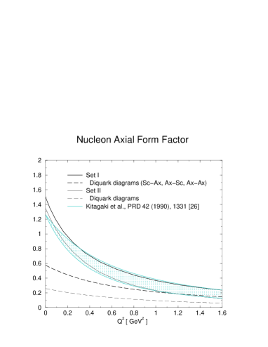
Figure 6: The pion-nucleon form factor $g_{\pi NN}(Q^{2})$ and the axial form factor $g_{A}(Q^{2})$. ’Diquark diagrams’ labels the sum of the impulse approximate axialvector contributions and scalar-axialvector transitions. The shaded region in the right panel represents the uncertainty in $g_{A}$ as determined from quasi-elastic neutrino scattering when a dipole form is fitted to both, the vector and the axial form factor Kit90 .

5 Summary and Conclusions

The description of baryons as fully relativistic bound states of quark and glue reduces to an effective Bethe-Salpeter (BS) equation with quark-exchange interaction when irreducible 3-quark interactions are neglected and separable 2-quark (diquark) correlations are assumed. By including axialvector diquark correlations with non-trivial quark substructure, we solved the BS equations of this covariant quark-diquark model for nucleons and the $\Delta$-resonance. While the $\Delta$ cannot be described without axialvector diquarks, the nucleon-$\Delta$ mass splitting imposes an upper bound on their relative importance inside nucleons, as compared to the scalar diquark correlations. At present, this bound seems somewhat too strong for a simultaneous description of octet and decuplet baryons in a fully satisfactory manner.

We furthermore extended previous studies of nucleon properties within the covariant quark-diquark model. In this way we assess the influence of the axialvector diquark correlations with non-trivial quark substructure. Electromagnetic form factors, the weak form factor $g_{A}$ and the strong form factor $g_{\pi NN}$ have been computed. Structures and strengths of the otherwise unknown axialvector diquark couplings, and of scalar-axialvector transitions, have thereby been obtained by resolving the quark-loop substructure of the diquarks at vanishing momentum transfer ($Q^{2}\to 0$).

An excellent description is obtained for the electric form factors of both nucleons. The ratio of the proton electric and magnetic moment, $\mu_{p}\,G_{E}/G_{M}$ as recently measured at TJNAF Jon99 , is well described with axialvector diquark correlations of moderate strength. Our results clearly indicate that axialvector diquarks are necessary to reproduce the qualitative behavior of the experimental data for this ratio. At the same time, an upper bound on the relative importance of axialvector diquarks and scalar-axialvector transitions (together of estimated 30% to the BS norm of the nucleons) can be inferred.

For axialvector correlations of such a strength, the phenomenological value for the isoscalar magnetic moment of the nucleons is well reproduced. The isovector contribution results around 15% too small. While the axialvector diquarks lead to a considerable improvement, both magnetic moments tend to be around 50% too small with scalar diquarks alone Oet99 , this remaining 15% mismatch in the isovector magnetic moment seems to be due to other effects. One possibility might be provided by vector diquarks. While their contributions to the binding energy of the nucleons are expected to be negligible, the photon couplings with vector diquarks could be strong enough to compensate this and thus lead to sizeable effects, in particular, in the magnetic moments.

For the pion-nucleon and the axial coupling constant, we found moderate violations of PCAC and the Goldberger-Treiman relation. For scalar diquarks alone, this is attributed to some violations of the (partial) conservation of the simplified axial current neglecting exchange quark couplings and chiral seagulls. Maintaining axialvector diquarks, additional PCAC violations can arise from missing vector diquarks which mix with the axialvectors under chiral transformations as pointed out in ref. Ish00 . This explains why the weaker axialvector correlations lead to better values for $g_{A}(0)$ and $g_{\pi NN}(0)$. Nevertheless, these violations are reasonably small and occur only at small momentum transfers $Q^{2}$. The axial form factor $g_{A}(Q^{2})$ is otherwise in good agreement with the experimental bounds from quasi-elastic neutrino scattering in Kit90 .

It should be noted that qualitatively the scalar-axialvector transitions are of particular importance to obtain values for $g_{A}>1$. These transitions thus solve a problem that previous applications of the covariant quark-diquark model shared with many chiral nucleon models. Their quantitative effect is somewhat too large, as discussed above.

The conclusions from our present study can be summarized as follows: While selected observables, sensitive to axialvector diquark correlations, can be improved considerably by their inclusion, other observables (and the nucleon-$\Delta$ mass splitting) provide upper bounds on their relative importance as compared to scalar diquarks. These bounds confirm that scalar diquarks provide for the dynamically dominant 2-quark correlations inside nucleons. Deviations of the order of 15% remain in the isovector part of the magnetic moment (too small), in $g_{A}(0)$ (too large) and in the Goldberger-Treiman relation. While these cannot be fully accounted for by including the axialvector diquark correlations, overall, however, the quark-diquark model was demonstrated to describe nucleon properties quite successfully.

Appendix A Resolving Diquarks

A.1  Electromagnetic Vertices

Here we adopt an impulse approximation to couple the photon directly to the quarks inside the diquarks obtaining the scalar, axialvector and the photon-induced scalar-axialvector diquark transition couplings as represented by the 3 diagrams in figure 2. For on-shell diquarks these yield diquark form factors and, under some mild assumptions on the quark-quark interaction kernel Oet99 , current conservation followed for amplitudes which solve a diquark BS equation. Due to the quark-exchange antisymmetry of the diquark amplitudes it suffices to calculate one diagram for each of the three contributions, i.e., those of figure 2 in which the photon couples to the “upper” quark line. The color trace yields one as in the normalization integrals, eqs. (7) and (8). The traces over the diquark flavor matrices with the charge matrix will be included implicitly in those over the Dirac structures in the resolved vertices which read (with the minus sign for fermion loops),

$$\tilde{\Gamma}^{\mu}_{sc} =-\text{Tr}\int\!\frac{d^{4}q}{(2\pi)^{4}} \bar{\chi}\left(\frac{\scriptstyle p_{2}-p_{3}}{\scriptstyle 2}\right)S(p_{2})(-i\gamma^{\mu})S(p_{1})\;\times$$ (49)

$$\chi\left(\frac{\scriptstyle p_{1}-p_{3}}{\scriptstyle 2}\right)S^{T}(p_{3})\;,$$

$$\tilde{\Gamma}^{\mu,\alpha\beta}_{ax} =-\text{Tr}\int\!\frac{d^{4}q}{(2\pi)^{4}} \bar{\chi}^{\alpha}\left(\frac{\scriptstyle p_{2}-p_{3}}{\scriptstyle 2}\right)S(p_{2})(-i\gamma^{\mu})S(p_{1})\;\times$$ (50)

$$\chi^{\beta}\left(\frac{\scriptstyle p_{1}-p_{3}}{\scriptstyle 2}\right)S^{T}(p_{3})\;,$$

$$\tilde{\Gamma}^{\mu,\beta}_{sa} =-\text{Tr}\int\!\frac{d^{4}q}{(2\pi)^{4}} \bar{\chi}\left(\frac{\scriptstyle p_{2}-p_{3}}{\scriptstyle 2}\right)S(p_{2})(-i\gamma^{\mu})S(p_{1})\;\times$$ (51)

$$\chi^{\beta}\left(\frac{\scriptstyle p_{1}-p_{3}}{\scriptstyle 2}\right)S^{T}(p_{3})$$

$$=2im_{q}\epsilon^{\mu\beta\rho\lambda} (p_{d}+k_{d})^{\rho}Q^{\lambda}\;\times$$

$$\int\!\frac{d^{4}q}{(2\pi)^{4}}\frac{g_{s}g_{a}\;P(q-Q/4)P(q+Q/4)}{(p_{1}^{2}+m_{q}^{2})(p_{2}^{2}+m_{q}^{2})(p_{3}^{2}+m_{q}^{2})}\;.$$

The quark momenta herein are,

$$p_{1} = \frac{p_{d}+k_{d}}{4}-\frac{Q}{2}+q\;,\quad p_{2}=\frac{p_{d}+k_{d}}{4}+\frac{Q}{2}+q\;,\quad$$

$$p_{3} = \frac{p_{d}+k_{d}}{4}-q\;.$$ (53)

Even though current conservation can be maintained with these vertices on-shell, off-shell $\tilde{\Gamma}^{\mu}_{sc}$ and $\tilde{\Gamma}^{\mu,\alpha\beta}_{ax}$ do not satisfy the Ward-Takahashi identities for the free propagators in eqs. (2,3). They can thus not directly be employed to couple the photon to the diquarks inside the nucleon without violating gauge invariance. For $Q=0$, however, they can be used to estimate the anomalous magnetic moment $\kappa$ of the axialvector diquark and the strength of the scalar-axialvector transition, denoted by $\kappa_{sa}$ in (29), as follows:

First we calculate the contributions of the scalar and axialvector diquark to the proton charge, i.e. the second diagram in figure 1 to $G_{E}(0)$, with replacing the vertices $\Gamma^{\mu}_{sc}$ and $\Gamma^{\mu,\alpha\beta}_{ax}$ given in eqs. (27) and (28) by the resolved ones, $\tilde{\Gamma}^{\mu}_{sc}$ and $\tilde{\Gamma}^{\mu,\alpha\beta}_{ax}$ in eqs. (49) and (50). Since the bare vertices on the other hand satisfy the Ward-Takahashi identities, and since current conservation is maintained in the calculation of the electromagnetic form factors, the correct charges of both nucleons are guaranteed to result from the contributions to $G_{E}(0)$ obtained with these bare vertices, $\Gamma^{\mu}_{sc}$ and $\Gamma^{\mu,\alpha\beta}_{ax}$ of eqs. (27) and (28). In order to reproduce the these correct contributions, we then adjust the values for the diquark couplings, $g_{s}$ and $g_{a}$, to be used in connection with the resolved vertices of eqs. (49) and (50). This yields couplings $g_{s}^{resc}$ and $g^{resc}_{a}$, slightly rescaled (by a factor of the order of one, see table 6). Once these are fixed we can continue and calculate the contributions to the magnetic moment of the proton that arise from the resolved axialvector and transition couplings, $\tilde{\Gamma}^{\mu,\alpha\beta}_{ax}$ and $\tilde{\Gamma}^{\mu,\beta}_{sa}$, respectively. These contributions determine the values of the constants $\kappa$ and $\kappa_{sa}$ for the couplings in eqs. (28) and (29), (30).

The results are given in table 6. As can be seen, the values obtained for $\kappa$ and $\kappa_{sa}$ by this procedure are insensitive to the parameter sets for the nucleon amplitudes. In the calculations of observables we use $\kappa=1.0$ and $\kappa_{sa}=2.1$.

	$g_{s}^{resc}/g_{s}$	$g_{a}^{resc}/g_{a}$	$\kappa$	$\kappa_{sa}$
Set I	0.943	1.421	1.01	2.09
Set II	0.907	3.342	1.04	2.14

Table 6: Rescaled diquark normalizations and constants of photon-diquark couplings.

A.2 Pseudoscalar and Pseudovector Vertices

The pion and the pseudovector current do not couple to the scalar diquark. Therefore, in both cases only those two contributions have to be computed which are obtained from the middle and lower diagrams in figure 2 with replacing the photon-quark vertex by the pion-quark vertex of eq. (36), and by the pseudovector-quark vertex of eq. (42), respectively. For Dirac part of the vertex describing the pion coupling to the axialvector diquark this yields,

$$\tilde{\Gamma}^{\rho\lambda}_{5,ax} =- 2\frac{m_{q}^{2}}{f_{\pi}}\epsilon^{\rho\lambda\mu\nu}(p_{d}+k_{d})^{\mu}Q^{\nu}\;\times$$

$$\int\!\frac{d^{4}q}{(2\pi)^{4}}\frac{g_{a}^{2}\;P(q-Q/4)P(q+Q/4)}{(p_{1}^{2}+m_{q}^{2})(p_{2}^{2}+m_{q}^{2})(p_{3}^{2}+m_{q}^{2})}\;,$$

and fixes its strength (at $Q^{2}=0$) to $\kappa_{ax}^{5}\approx 4.5$, see table 7.

For the effective pseudovector-axialvector diquark vertex in eq. (45) it is sufficient to consider the regular part, since its pion pole contribution is fully determined by eq. (A) already. The regular part reads,

$$\tilde{\Gamma}^{\mu\rho\lambda}_{5,ax} = \int\!\frac{d^{4}q}{(2\pi)^{4}}\frac{g_{a}^{2}\;P(q-Q/4)P(q+Q/4)}{(p_{1}^{2}+m_{q}^{2})(p_{2}^{2}+m_{q}^{2})(p_{3}^{2}+m_{q}^{2})}\;\times$$

$$\left[-4m_{q}^{2}\epsilon^{\mu\rho\lambda\nu}\;(p_{1}+p_{2}+p_{3})^{\nu}-\text{Tr}\gamma_{5}\gamma^{\rho}p/\hskip 1.34995pt_{2}\gamma^{\mu}p/\hskip 1.34995pt_{1}\gamma^{\lambda}p/\hskip 1.34995pt_{3}\right].$$

Although after the $q$-integration, the terms in brackets yield the four independent Lorentz structures discussed in the paragraph above eq. (45), only the first term contributes to $g_{A}(0)$ (with $p_{1}+p_{2}+p_{3}=(3/4)(p_{d}+k_{d})+q$).

The scalar-axialvector transition induced by the pion is described by the vertex

$$\tilde{\Gamma}^{\rho}_{5,sa} = 4i\frac{m_{q}}{f_{\pi}}\int\!\frac{d^{4}q}{(2\pi)^{4}}g_{s}g_{a}\;P(q-Q/4)P(q+Q/4)\;\times$$

$$\qquad\frac{(p_{2}p_{3})p_{1}^{\rho}-(p_{3}p_{1})p_{2}^{\rho}+(p_{1}p_{2})p_{3}^{\rho}}{(p_{1}^{2}+m_{q}^{2})(p_{2}^{2}+m_{q}^{2})(p_{3}^{2}+m_{q}^{2})},$$

and the reverse (axialvector-scalar) transition is obtained by substituting $Q\rightarrow-Q$ (or $p_{1}\leftrightarrow p_{2}$) in (A). The corresponding vertex for the pseudovector current reads

$$\tilde{\Gamma}^{\mu\rho}_{5,sa} =-4im_{q} \int\!\frac{d^{4}q}{(2\pi)^{4}}\frac{g_{s}g_{a}\;P(q-Q/4)P(q+Q/4)}{(p_{1}^{2}+m_{q}^{2})(p_{2}^{2}+m_{q}^{2})(p_{3}^{2}+m_{q}^{2})}\times$$

$$\left[\delta^{\mu\rho}(m_{q}^{2}-p_{1}p_{2}-p_{2}p_{3}-p_{3}p_{1})\;+\right.$$

$$\left.\;\{p_{1}p_{2}\}_{+}^{\mu\rho}+\{p_{1}p_{3}\}_{+}^{\mu\rho}-\{p_{2}p_{3}\}_{-}^{\mu\rho}\right].$$

The short-hand notation for a(n) (anti)symmetric product used herein is defined as $\{p_{1}p_{2}\}_{\pm}^{\mu\nu}=p_{1}^{\mu}p_{2}^{\nu}\pm p_{1}^{\nu}p_{2}^{\mu}$. The reverse transition is obtained from $Q\rightarrow-Q$ together with an overall sign change in (A). As already mentioned in the main text, the term proportional to $\delta^{\mu\nu}$ provides 99 per cent of the value for $g_{A}$ as obtained with the full vertex. It therefore clearly represents the dominant tensor structure.

	$\kappa^{5}_{ax}$	$\kappa^{5}_{\mu,ax}$	$\kappa^{5}_{sa}$	$\kappa^{5}_{\mu,sa}$
Set I	4.53	4.41	3.97	1.97
Set II	4.55	4.47	3.84	2.13

Table 7: Strengths for pion– and pseudovector-diquark couplings.

As explained for the electromagnetic couplings of diquarks, we use these resolved vertices in connection with the rescaled couplings $g_{s}^{resc}$ and $g_{a}^{resc}$ to compute $g_{\pi NN}$ and $g_{A}$ in the limit $Q\rightarrow 0$. In this way the otherwise unknown constants that occur in the (pointlike) vertices of eqs. (44–47) are determined.

As seen from the results in table 7, the values obtained for these effective coupling constants are only slightly dependent on the parameter set (the only exception being $\kappa^{5}_{\mu,sa}$ where the two values differ by 8%). For the form factor calculations presented in Sec. 3 we employ $\kappa^{5}_{ax}=4.5$, $\kappa^{5}_{\mu,ax}=4.4$, $\kappa^{5}_{sa}=3.9$ and $\kappa^{5}_{\mu,sa}=2.1$.

References

- (1)
- (2) H. Leutwyler and J. Stern, Annals Phys. 112 (1978) 94.
- (3) A. Szczepaniak, C. R. Ji and S. R. Cotanch, Phys. Rev. C52 (1995) 2738.
- (4) P. L. Chung and F. Coester, Phys. Rev. D44 (1991) 229.
- (5) S. Capstick and B. Keister, Phys. Rev. D51 (1995) 3598.
- (6) F. Cardarelli, E. Pace, G. Salme and S. Simula, Phys. Lett. B357 (1995) 267.
- (7) S. Boffi, P. Demetriou, M. Radici and R. F. Wagenbrunn, Phys. Rev. C60 (1999) 025206.
- (8) G. Hellstern, R. Alkofer, M. Oettel and H. Reinhardt, Nucl. Phys. A627 (1997) 679.
-
(9)
J. C. Bloch et al.,
Phys. Rev. C60 (1999) 062201;
J. C. Bloch, C. D. Roberts and S. M. Schmidt, Phys. Rev. C61 (2000) 065207;
M. B. Hecht, C. D. Roberts and S. M. Schmidt, nucl-th/0005067. - (10) M. Oettel, M. A. Pichowsky and L. von Smekal, nucl-th/9909082, Eur. Phys. J. A8 (2000) in press.
- (11) A. N. Kvinikhidze and B. Blankleider, Phys. Rev. C60 (1999) 044003; ibid. 044004.
- (12) N. Ishii, e-print, nucl-th/0004063.
- (13) K. Kusaka, G. Piller, A. W. Thomas and A. G. Williams, Phys. Rev. D55 (1997) 5299.
- (14) M. Oettel, G. Hellstern, R. Alkofer and H. Reinhardt, Phys. Rev. C58 (1998) 2459.
- (15) M. Oettel and R. Alkofer, Phys. Lett. B484 (2000) 243.
- (16) A. Bender, C. D. Roberts and L. v. Smekal, Phys. Lett. B380 (1996) 7.
- (17) P. Maris, C. D. Roberts and P. C. Tandy, Phys. Lett. B420 (1998) 267.
- (18) P. Maris and C. D. Roberts, Phys. Rev. C56 (1997) 3369.
- (19) R. Delbourgo and M. D. Scadron, J. Phys. G5 (1979) 1621.
- (20) S. Kopecky, P. Riehs, J. A. Harvey and N. W. Hill, Phys. Rev. Lett. 74 (1995) 2427.
- (21) G. Hoehler et al., Nucl. Phys. B114 (1976) 505.
- (22) S. Platchkov et al., Nucl. Phys. A510 (1990) 740.
- (23) I. Passchier et al., Phys. Rev. Lett. 82 (1999) 4988.
- (24) M. Ostrick et al., Phys. Rev. Lett. 83 (1999) 276.
- (25) M. K. Jones et al. [Jefferson Lab Hall A Collaboration], Phys. Rev. Lett. 84 (2000) 1398.
- (26) R. A. Arndt, R. L. Workman and M. M. Pavan, Phys. Rev. C49 (1994) 2729.
- (27) J. Rahm et al., Phys. Rev. C57 (1998) 1077.
- (28) C. Caso et al., Review of Particle Physics, Eur. Phys. J. C3 (1998) 1.
- (29) T. Kitagaki et al., Phys. Rev. D42 (1990) 1331.