MKPH-T-00-08
Analysis of the low-energy $\eta$NN-dynamics within a three-body formalism

Abstract

The interaction of an $\eta$-meson with two nucleons is studied within a three-body approach. The major features of the $\eta NN$-system in the low-energy region are accounted for by using a $s$-wave separable ansatz for the two-body $\eta N$- and $NN$-amplitudes. The calculation is confined to the $(J^{\pi};T)=(0^{-};1)$ and $(1^{-};0)$ configurations which are assumed to be the most promising candidates for virtual or resonant $\eta NN$-states. The eigenvalue three-body equation is continued analytically into the nonphysical sheets by contour deformation. The position of the poles of the three-body scattering matrix as a function of the $\eta N$-interaction strength is investigated. The corresponding trajectory, starting on the physical sheet, moves around the $\eta NN$ three-body threshold and continues away from the physical area giving rise to virtual $\eta NN$-states. The search for poles on the nonphysical sheets adjacent directly to the upper rim of the real energy axis gives a negative result. Thus no low-lying $s$-wave $\eta NN$-resonances were found. The possible influence of virtual poles on the low-energy $\eta NN$-scattering is discussed.

PACS numbers: 13.60.Le, 21.45.+v, 25.20.Lj

I Introduction

The low-energy interaction of $\eta$-mesons with few-nucleon systems has recently become the subject of vigorous investigations. A great deal of attention has been devoted to the search for possible bound or resonance states in these systems. After an experimental study at Brookhaven [1], which casts some doubt upon the possibility of observing $\eta$-nuclei with relatively large mass numbers A$\geq$12, the attention was redirected to the interaction of $\eta$-mesons with light nuclei [2, 3, 4, 5, 6, 7]. Recent theoretical investigations have mainly been stimulated by the precise measurements of the photoproduction and hadronic reactions with $\eta$-mesons in final states. The obtained results are often interpreted as strong experimental hints that correlated states for light $\eta$-nuclear systems might exist (see e.g. [8]). The case in point is the strong energy dependence of the experimental cross sections observed near the $\eta$-production threshold [9, 10].

In the present work we deal primarily with the dynamical properties of the $\eta NN$-system. The understanding of these properties is important for the following reasons. Firstly, the $\eta NN$-system is interesting in itself. It is the simplest $\eta$-nuclear system which admits an exact solution within the three-body formalism. Furthermore, it may be regarded as an example of a three-body system in which the pairwise driving forces are attractive and which may in principle develop a bound (or virtual) state, or a low-energy three-particle resonance near zero energy. Secondly, the study of $\eta NN$-scattering may serve as a promising tool for the investigation of the corresponding processes in complex nuclei. The possible existence of such correlated objects would point to the crucial significance of two-nucleon mechanisms in the $\eta$-interaction with nuclei. This fact in turn would require the revision of the simple first order approximation to the $\eta$-nuclear optical potential adopted by the currently available models [11, 12, 13].

The main features of the $\eta NN$-dynamics in a quasideuteron state of spin, parity and isospin $(J^{\pi};T)=(1^{-};0)$ are already elucidated in the literature. Ueda was the first to carry out an extensive calculation of $\eta d$-scattering within a three-body approach [2] and found that the $\eta d$-system can form a quasi-bound state with a mass of 2430 MeV and a rather small width of about 10-20 MeV. Other calculations, also looking for bound or resonant $\eta d$-states within the Faddeev theory, have recently been reported by Shevchenko et al. [4] as well as by Garcilazo and Peña [5]. The authors of Ref.[4] confirmed qualitatively the results of [2] and fixed the values of the $\eta N$-scattering length for which the previously bound $\eta d$-state becomes a low-lying $s$-wave resonance. In Ref.[5] the possible existence of $\eta d$ bound states within the different $\eta N$- and $NN$-interaction models is also studied. As for the experimental investigations, we would like to mention the measurements presented in [10] for the reaction $np\to\eta d$ where a visible increase of the $\eta$-meson yield over the mere phase-space calculation was observed near threshold. Recently, Metag et al. [9] have reported new results for the cross section $\gamma d\to\eta X$. These authors also note a strong enhancement of events in the energy region of a few MeV above threshold. Such a feature cannot be explained within the truncated multiple scattering approach developed in [14], where only single $\eta N$- and $NN$-rescatterings were included in the calculation as the most important corrections to the impulse approximation. This discrepancy is not surprising, since the validity of the latter approach is associated with the short range nature of the $\eta N$- and $NN$-interactions in relation to the characteristic internucleon distance in the deuteron. In this situation, when thinking about the whole picture of the $\eta NN$ dynamics, one may assume that, when the attractive forces pull all particles together so that the two-body potentials overlap, qualitatively new features of the resulting $\eta NN$-interaction may be expected.

In this paper we will study the question whether the dynamical properties of the $\eta NN$-system allow the existence of a bound (or virtual) state or a three-body resonances in the low-energy region. Although this question has already been covered partially in the above mentioned works [2, 4, 5] we would like to reinvestigate it using a fundamentally different method, based on a search for poles of the scattering matrix in the complex energy plane. It possesses several important advantages over the conventional procedure of solving the on-shell Faddeev equation. Besides being more convenient for determining the exact position of $S$-matrix poles, the method provides additional insights into the source of appearance of these poles close to the physical domain. Furthermore, this approach allows us to investigate the $(J^{\pi};T)=(0^{-};1)$ state which is not touched upon in the literature to the best of our knowledge. As was established in [14], this configuration plays the dominant role in the final state of the $\gamma d\to\eta X$ reaction near threshold. Therefore, if one attributes the anomalous behaviour of the $\gamma d\to\eta X$ cross section reported in [9] to a near lying $S$-matrix pole, one has to search it in the $(J^{\pi};T)=(0^{-};1)$ state. Broadly speaking, in view of the exclusive character of the measurements [9], the marked enhancement of the near threshold yield can be assigned to the $\eta d$ final state. But the simple estimation shows that in order to explain the observed results one would need an enhancement factor of about 30 what in our opinion seems unlikely. In this context, large attention is focussed on the $(J^{\pi};T)=(0^{-};1)$ configuration in this paper.

Our principal tool is the three-body approach realized within the Alt-Grassberger-Sandhas formalism [15]. Since the search for the $S$-matrix poles requires the analytical continuation of the dynamical equation into the nonphysical sheets of the Riemann surface, the analytical form for the driving two-body interactions is needed. For this reason, we use a simple separable potential of rank one and restrict our consideration to only $s$-waves in the two-body subsystems. This approach is well justified by the empirically established $s$-wave dominance of the low-energy $\eta N$- and $NN$- scattering. There exist strong experimental and theoretical evidences that the low-energy $\eta N$-interaction is dominated by the formation of the $S_{11}$(1535) resonance. Analogously, the ${}^{1}S_{0}$ and ${}^{3}S_{1}$ poles determine to a large extent the nucleon-nucleon low-energy interaction. Thus the $s$-wave isobars in the $\eta N$ and $NN$ two-body channels are expected to be the main source of the $\eta NN$-forces. Therefore we hope that our separable model, though being quite simple, will reproduce the major features of the $\eta NN$-dynamics.

In Sect. II we briefly describe the three-body scattering formalism pertinent to the present problem. Some details connected with the driving two-body interactions as well as the main calculational formulas are given in Sect. III. In Sect. IV the procedure of analytical continuation of the scattering equation into nonphysical energy sheets is described and the strategy for the search of the $S$-matrix poles is presented. The discussion of our main results and the conclusions are presented in the last two sections.

II General formalism

In this section we will briefly review the properties of the three-body equation which will concern us in the remainder of this paper. Our starting point is the conventional three-body scattering theory in AGS form [15]. The three channels comprising two interacting particles and one spectator are labeled according to the number of the spectator. As already mentioned in the introduction, we take for each channel as the off-shell two-body $t$-matrix a rank-one ansatz

$$t_{k}(E)=|f_{k}\rangle\tau_{k}(E)\langle f_{k}|\,,$$ (1)

and we will call such an interacting pair in the following “isobar”. Here $|f_{k}\rangle$ is the vertex function, and the isobar propagator $\tau_{k}$ is defined as

$$\tau_{k}(E)=\frac{\gamma_{k}}{1-\gamma_{k}\langle f_{k}|G_{k}^{(2)}(E)|f_{k}\rangle}\,,$$ (2)

where $G_{k}^{(2)}(E)$ denotes the free two-body Green’s function with $E$ as total c.m. energy of the two-particle system. The separable form (1) enables one to reduce the three-body problem to a set of coupled effective two-body equations for the transition amplitudes $X_{ij}$

$$X_{ij}(W)=(1-\delta_{ij})Z_{ij}(W)+\sum\limits_{k=1}^{3}(1-\delta_{ik})Z_{ik}(W)\tau_{k}(E_{k})X_{kj}(W)\,,\quad(i,j=1,2,3)\,,$$ (3)

where $W$ denotes the total three-body energy while the isobar propagator $\tau_{k}$ depends explicitly on the invariant energy $E_{k}$ of the two-body subsystem, which is a function of $W$ and the kinetic energy of the spectator. The energy dependent driving terms are

$$Z_{ij}(W)=\langle f_{i}|G(W)|f_{j}\rangle\,,$$ (4)

with $G(W)$ being the free three-body Green’s function. When evaluating equation (4) in momentum space and making a partial wave decomposition, it becomes a set of one-dimensional integral equations of Fredholm type. It is known that for an inhomogeneous Fredholm equation to be singular, in which case the transition matrix $X_{ij}$ has a pole, it is necessary and sufficient for the corresponding homogeneous equation

$$F_{ij}(W)=\sum\limits_{k=1}^{3}(1-\delta_{ik})Z_{ik}(W)\tau_{k}(E_{k})F_{kj}(W)\,,\quad(i,j=1,2,3)\,$$ (5)

to have a nonzero solution for the same value of the parameter $W$. Thus the problem of searching for poles of the scattering matrix reduces to that of finding those values $W$ for which the Fredholm determinant $D(W)$ of (3) vanishes

$$D(W)=0\,.$$ (6)

We now turn to the $\eta NN$-system for which we adopt the labeling $k=1,2$ for a nucleon spectator and $k=3$ for the $\eta$ spectator, and furthermore change the channel notation as

$$\begin{array}[]{cl}1=2\rightarrow N^{*}&\mbox{ for the }\eta N\mbox{-isobar plus spectator nucleon}\,,\cr 3\rightarrow d&\mbox{ for the $NN$-isobar plus spectator meson}.\cr\end{array}$$ (7)

The identity of the channels 1 and 2 reduces the 3$\times$3 system (5) to a 2$\times$2 system which has the following operator form in our new notation

$$F_{dd}=2Z_{dN^{*}}\tau_{N^{*}}F_{N^{*}d}\,,$$ (8)

$$F_{N^{*}d}=Z_{N^{*}d}\tau_{d}F_{dd}+Z_{N^{*}N^{*}}\tau_{N^{*}}F_{N^{*}d}\,,$$ (9)

$$F_{dN^{*}}=2Z_{dN^{*}}\tau_{N^{*}}F_{N^{*}N^{*}}\,,$$ (10)

$$F_{N^{*}N^{*}}=Z_{N^{*}d}\tau_{d}F_{dN^{*}}+Z_{N^{*}N^{*}}\tau_{N^{*}}F_{N^{*}N^{*}}\,.$$ (11)

A close examination of (8) through (11) reveals that we have two decoupled sets of coupled equations sharing the identical integration kernel. Indeed, the coupled equations (8) and (9) are transformed into (10) and (11) by the substitutions $F_{dd}\rightarrow F_{dN^{*}}$ and $F_{N^{*}d}\rightarrow F_{N^{*}N^{*}}$. Therefore, it is sufficient to consider only one set for which we choose the second one. After inserting (10) into (11) the former equation may be written in the closed form

$$F_{N^{*}N^{*}}=(Z_{N^{*}N^{*}}+2Z_{N^{*}d}\tau_{d}Z_{dN^{*}})\,\tau_{N^{*}}F_{N^{*}N^{*}}.\\$$ (12)

It is diagrammatically presented in Fig. 1. In analogy to a homogeneous Lippmann-Schwinger equation, we see that the driving term $Z_{N^{*}N^{*}}$ plays the role of a meson exchange $NN^{*}$-potential while the second term in brackets gives the mechanism associated with intermediate $NN$-interaction where the $\eta$ acts as a spectator.

III Two-body ingredients

Now we will specify the separable $\eta N$ and $NN$ scattering matrices which determine the driving two-body forces in our model. Since we restrict the pair-interaction to $s$-waves only, the vertex functions have a simple structure determined by two parameters, the coupling constant $g_{k}$ and the cut-off $\beta_{k}$

$$\langle\vec{p}\,|f_{k}\rangle=f_{k}(p)=g_{k}\,F_{k}(p)\,\mbox{ with }\,F_{k}(p)=\frac{\beta_{k}^{2}}{\beta_{k}^{2}+p^{2}}\,,$$ (13)

where $\vec{p}$ denotes the relative momentum of the interacting pair.

For the $s$-wave $t$-matrix of the $NN=d$ isobar

$$t_{d}(p,p^{\prime},E_{d})=f_{d}(p)\tau_{d}(E_{d})f_{d}(p^{\prime})\,,$$ (14)

the following parametrization has been used

$$g_{d}^{2}=\frac{16\pi a}{a\beta_{d}-2}\,,\quad\gamma_{d}=-\frac{1}{2M_{N}}\,,$$ (15)

where $a$ is the $NN$-scattering length. For the propagator $\tau_{d}$ one then obtains

$$\tau_{d}(E_{d})=-\frac{1}{2M_{N}}\,\Big{[}1+\frac{g_{d}^{2}\beta_{d}^{3}}{16\pi\left(i\beta_{d}+\sqrt{M_{N}(E_{d}-2M_{N})}\right)^{2}}\Big{]}^{-1}\,.$$ (16)

The $NN$-interaction parameters were taken from the low-energy $np$-scattering fit of Yamaguchi [16]

$$\beta_{d}=1.4488\,\mbox{fm}^{-1},\quad a=\left\{\begin{array}[]{rl}5.378\,\mbox{fm}&\mbox{for the ${}^{3}S_{1}$-state,}\cr-23.690\,\mbox{fm}&\mbox{for the ${}^{1}S_{0}$-state.}\cr\end{array}\right.$$ (17)

Analogously, we use for the $\eta N$=$N^{*}$ $t$-matrix the following ansatz

$$t_{N^{*}}(p,p^{\prime},E_{N^{*}})=f^{(\eta)}_{N^{*}}(p)\tau_{N^{*}}(E_{N^{*}})f^{(\eta)}_{N^{*}}(p^{\prime})\,.$$ (18)

Here the $N^{*}$-propagator is given in the form

$$\tau_{N^{*}}(E_{N^{*}})=\Big{(}E_{N^{*}}-M_{0}-\Sigma_{\pi}(E_{N^{*}})-\Sigma_{\eta}(E_{N^{*}})\Big{)}^{-1}\,,$$ (19)

where $M_{0}$ denotes the bare mass of the $S_{11}$(1535)-resonance. The resonance self energies associated with the couplings to the $\pi N$ and $\eta N$ channels are determined by

$$\Sigma_{j}(E_{N^{*}})=\frac{1}{2\pi^{2}}\int\limits_{0}^{\infty}\frac{f^{(j)2}_{N^{*}}(p)}{E_{N^{*}}-E_{N}(p)-\omega_{j}(p)+i\epsilon}\ \frac{p^{2}\,dp}{2\,\omega_{j}(p)}\,,$$ (20)

where $\omega_{j}(p)=\sqrt{m_{j}^{2}+p^{2}}$ denotes the energy of meson “$j$” and $E_{N}(p)=M_{N}+p^{2}/2M_{N}$ is the nonrelativistic total nucleon energy. The meson-$N^{*}$ vertices are defined by $(j=\pi,\eta)$

$$f^{(j)}_{N^{*}}(p)=g^{(j)}_{N^{*}}\,F_{N^{*}}^{(j)}(p)\,,\quad\mbox{with}\quad F_{N^{*}}^{(j)}(p)=\frac{\beta_{N^{*}}^{(j)2}}{\beta_{N^{*}}^{(j)2}+p^{2}}\,.$$ (21)

The $N^{*}$ parameters were chosen in such a way that the main ratios of the hadronic decays of the $S_{11}$(1535) resonance are reproduced. We have taken

$$g_{N^{*}}^{(\eta)}=2.0\,,\ g_{N^{*}}^{(\pi)}=1.5\,,\ \beta_{N^{*}}^{(\eta)}=6.5\,\mbox{fm}^{-1},\ \beta_{N^{*}}^{(\pi)}=4.5\,\mbox{fm}^{-1}.$$ (22)

The bare $S_{11}$ mass $M_{0}$ was determined by the condition

$$M_{0}+\Re e\Big{(}\Sigma_{\pi}(M^{*})+\Sigma_{\eta}(M^{*})\Big{)}=M^{*}\,,$$ (23)

where $M^{*}=1535$ MeV is the mass of the dressed isobar. The choice (22) gives for the total and partial decay widths at the resonance position

$$\Gamma=150\,\mbox{MeV},\quad\frac{\Gamma_{\eta N}}{\Gamma}=\frac{\Gamma_{\pi N}}{\Gamma}=0.5\,,$$ (24)

which is reasonably consistent with the values given in the 1998 Particle Data Group listings [17].

For the actual evaluation of (12) we use a natural representation in which the total angular momentum $J$ and the total isospin $T$ are diagonal. The $\eta NN$ wave function is expanded into a complete set of the following basis states

$$|\vec{q}\,;\,JM_{J}\,TM_{T}\rangle = |\{(\tau_{i}\tau_{j})t_{k}\tau_{k}\}TM_{T}\rangle\,\sum\limits_{LM_{L}}\sum\limits_{SM_{S}}C_{LM_{L}\,SM_{S}}^{JM_{J}}\,|\{(\sigma_{i}\sigma_{j})s_{k}\sigma_{k}\}SM_{S}\rangle\,|q;\,LM_{L}\rangle\,Y_{LM_{L}}(\hat{q})\,.$$ (25)

Here $\sigma_{i}$ and $\tau_{i}$ denote the spin and isospin of the individual particles forming the isobar with the corresponding quantum numbers $s_{i}$ and $t_{i}$. The partial waves are normalized as

$$\langle q;\,LM_{L}|q^{\prime};\,L^{\prime}M^{\prime}_{L}\rangle=\frac{1}{q^{2}}\delta(q-q^{\prime})\delta_{L^{\prime}L}\delta_{M^{\prime}_{L}M_{L}}\,.$$ (26)

In (25) we have already taken into account that the two-particle forces act only in $l=0$ states. The momentum $\vec{q}$ characterizes the relative motion of the correlated $(ij)$-pair and a spectator particle. It is projected onto the partial waves specified by the total orbital momentum $L$ with projection $M_{L}$. Taking into account the parametrization adopted for the two-body vertices, the expansion (25) turns the operator equation (12) into a set of one-dimensional integral equations for the partial waves $|q;\,LM_{L}\rangle$. In the following we consider only states with total orbital angular momentum $L=0$. Then the two allowed configurations are $(J^{\pi};T)=(0^{-};1)$ and $(1^{-};0)$. Consequently, only the ${}^{1}S_{0}$ $NN$-state contributes to the three-body state $(0^{-};1)$, and correspondingly the ${}^{3}S_{1}$ $NN$-state to $(1^{-};0)$.

In order to apply the representation (25) to Eq. (12), we only need the spin-isospin recoupling coefficients between the states $j$ and $k$ for which one has

$$\langle\{(\sigma_{i}\sigma_{j})s_{k}\sigma_{k}\}SM_{S}|\{(\sigma_{k}\sigma_{i})s_{j}\sigma_{j}\}S^{\prime}M^{\prime}_{S}\rangle = \delta_{S^{\prime}S}\delta_{M^{\prime}_{S}M_{S}}\sqrt{(2s_{j}+1)(2s_{i}+1)}W(\sigma_{i}\sigma_{k}\sigma_{j}S;\,s_{j}s_{k})\,,$$ (27)

$$\langle\{(\tau_{i}\tau_{j})t_{k}\tau_{k}\}TM_{T}|\{(\tau_{k}\tau_{i})t_{j}\tau_{j}\}T^{\prime}M^{\prime}_{T}\rangle = \delta_{T^{\prime}T}\delta_{M^{\prime}_{T}M_{T}}\sqrt{(2t_{j}+1)(2t_{i}+1)}W(\tau_{i}\tau_{k}\tau_{j}T;\,t_{j}t_{k})\,,$$ (28)

where $W(j_{1}\,j_{2}\,j_{3}\,j_{4}\,;\,j_{5}\,j_{6})$ denotes the standard Racah coefficient.

Taking the actual quantum numbers of the participating particles, we obtain the following explicit form of the driving terms appearing in (12)

$$\langle\vec{p};\,JT|Z_{N^{*}N^{*}}|\vec{p}\,^{\prime};\,JT\rangle=V_{\eta}(p,p^{\prime},W)+\chi V_{\pi}(p,p^{\prime},W)\,.$$ (29)

Here the spin-isospin coefficients are $\chi=-1/3$ for $(0^{-};1)$ and $\chi=1$ for $(1^{-};0)$. The meson-exchange potential acting in the $L=0$ wave reads

$$V_{j}(p,p^{\prime},W)=\frac{g_{N^{*}}^{(j)2}}{8\pi}\int\limits_{-1}^{+1}\frac{F_{N^{*}}^{(j)}\Big{(}\vec{p}\,^{\prime}+\frac{M_{N}}{M_{N}+m_{j}}\vec{p}\Big{)}F_{N^{*}}^{(j)}\Big{(}\vec{p}+\frac{M_{N}}{M_{N}+m_{j}}\vec{p}\,^{\prime}\Big{)}}{2\omega_{j}(|\vec{p}+\vec{p}\,^{\prime}|)\,\Big{(}W-E_{N}(p)-E_{N}(p^{\prime})-\omega_{j}(|\vec{p}+\vec{p}\,^{\prime}|)\Big{)}}\,d(\hat{p}\cdot\hat{p}^{\prime})\,,$$ (30)

with $(j=\pi,\eta)$. For simplicity we use the nonrelativistic relative meson-nucleon momenta in the arguments of the regularization vertex form factors. The driving term associated with the intermediate $NN$-interaction has the form, using $E_{d}=W-\omega_{\eta}(q)-q^{2}/4M_{N}$ as the total c.m. energy of the interacting $NN$-pair,

$$\langle\vec{p}\,;\,JT|Z_{N^{*}d}\tau_{d}Z_{dN^{*}}|\vec{p}\,^{\prime};\,JT\rangle = V_{d}(p,p^{\prime},W)$$ (31)

$$= \frac{2}{\pi}\int\limits_{0}^{\infty}\frac{q^{2}\,dq}{2\omega_{\eta}(q)}\,V_{N}(p,q,W)\,\tau_{d}\Big{(}W-\omega_{\eta}(q)-q^{2}/4M_{N}\Big{)}\,V_{N}(p^{\prime},q,W)\,,$$ (32)

where the nucleon-exchange potential is given by

$$V_{N}(p,p^{\prime},W)=\frac{g_{N^{*}}^{(\eta)}g_{d}}{8\pi}\int\limits_{-1}^{+1}\frac{F_{N^{*}}^{(\eta)}\Big{(}\vec{p}\,^{\prime}+\frac{m_{\eta}}{M_{N}+m_{\eta}}\vec{p}\Big{)}\,F_{d}\Big{(}\vec{p}+\frac{\vec{p}\,^{\prime}}{2}\Big{)}}{W-E_{N}(p)-\omega_{\eta}(p^{\prime})-E_{N}(|\vec{p}+\vec{p}\,^{\prime}|)}\,d(\hat{p}\cdot\hat{p}^{\prime})\,.$$ (33)

The integrals in (30) and (33) can be evaluated analytically. The corresponding expressions, being rather cumbersome, are listed in the appendix. Finally, we present the partial wave representation of our basic homogeneous equation (12)

$$F_{N^{*}N^{*}}(p,W)=\frac{2}{\pi}\int\limits_{0}^{\infty}V_{N^{*}N^{*}}(p,p^{\prime},W)\,\tau_{N^{*}}(W-E_{N}(p^{\prime})-p^{\prime\,2}/2M^{*})\,F_{N^{*}N^{*}}(p^{\prime},W)\,p^{\prime}\,{}^{2}dp^{\prime}\,,$$ (34)

where the notation

$$V_{N^{*}N^{*}}(p,p^{\prime},W)=2V_{d}(p,p^{\prime},W)+V_{\eta}(p,p^{\prime},W)+\chi\,V_{\pi}(p,p^{\prime},W)$$ (35)

is introduced, and the invariant mass of the $N^{*}$-isobar in (35) was evaluated as $E_{N^{*}}=W-E_{N}(p^{\prime})-p^{\prime 2}/2M^{*}$. Anticipating a later result, we note that the contribution from the pion exchange potential $V_{\pi}$ in (35) is practically insignificant, and almost the whole attraction in the $\eta NN$-system comes from the first two terms with approximately equal strengths.

The method for searching the zeros of the Fredholm determinant $D(W)$ is to approximate the integral in Eq. (34) by a finite sum, transforming it into an ordinary matrix equation. Then (6) may be written as an algebraic equation

$$\det\Big{|}\delta_{ij}-\frac{2}{\pi}p_{j}^{2}C_{j}V_{N^{*}N^{*}}(p_{i},p_{j},W)\tau_{N^{*}}\Big{(}W-E_{N}(p_{j})-\frac{p_{j}^{2}}{2M^{*}}\Big{)}\Big{|}=0\,.$$ (36)

Here $C_{j}$ are the weights for the chosen quadrature (in the present calculation we have chosen the Gauss quadrature).

IV Structure of the Riemann surface and continuation into nonphysical sheets

Our main concern is to find the zeros of the Fredholm determinant in the complex energy plane resulting in poles of the scattering matrix. The structure of the manifold Riemann surface for the $\eta NN$-system in $(J^{\pi};T)=(1^{-};0)$ channel is presented in Fig. 2. Shown are the physical sheet $\Pi_{1}$ and the nearest nonphysical sheets $\Pi_{2}$, $\Pi_{3}$ directly adjacent to $\Pi_{1}$. The sheet $\Pi_{1}$ has a conventional analytical structure. Namely, it may have poles corresponding to a possible formation of three-body bound states, and the unitarity right-hand cuts. The former stem from the Cauchy type integrals inherent in the integration kernel in (34). There are two main cuts which determine the structure of the Riemann surface for the three-body problem in the energy region of interest:

(i) A two-particle cut, beginning at the two-body threshold $W_{\eta d}=2M_{N}+m_{\eta}+\epsilon_{d}$ where $\epsilon_{d}<0$ is the deuteron binding energy. The cut arises from the propagator $\tau_{d}(E_{d})$ which has a pole when $E_{d}-2M_{N}=\epsilon_{d}$. This pole is associated with the elastic $\eta$-deuteron scattering and gives the well known two-body contribution to the common three-body unitarity relations. The corresponding square-root branch point $W=W_{\eta d}$ develops the two-sheet structure $\{\Pi_{1},\,\Pi_{2}\}$ typical for conventional two-body scattering.

(ii) A three-body cut, starting at the three-body threshold $W_{\eta NN}=2M_{N}+m_{\eta}$. This cut is induced by the two-body right-hand cut in $\tau_{d}$ corresponding to the $d\to NN$ break-up and by the similar cut in $\tau_{N^{*}}$ associated with the decay $N^{*}\to\eta N$. The corresponding nonphysical sheet is denoted as $\Pi_{3}$ in Fig. 2. Furthermore, the driving terms $V_{\pi}$, $V_{\eta}$, and $V_{N}$ in (30) through (33) contain the well known logarithmic singularities which are analogous to the dynamical (left-hand) singularities of the nucleon-nucleon OBE potential and correspond to the exchange of a real particle which becomes possible when $W\geq W_{\eta NN}$. For some values of $p$ and $p^{\prime}$ these singularities pinch the real axis producing the additional three-body cut beginning at the branch point $W=W_{\eta NN}$. In the partial wave representation, this point is of logarithmic type and gives rise to an infinite number of sheets at $W=W_{\eta NN}$. The structure of the Riemann surface associated with the logarithmic singularities is in itself of no physical interest and is therefore not presented in Fig. 2.

All sheets are connected as depicted in Fig. 2. The sheet $\Pi_{2}$ may contain the poles which show-up as correlated two-body $\eta d$ states (virtual or resonant). The analogous states which may be observed in the three particle scattering processes are located on the sheet $\Pi_{3}$. In the absence of an actual three-body scattering experiment, these states may occur as final states in reactions with, e.g., deuteron break-up, such as $\gamma d\to\eta np$. Following the terminology accepted in the literature we call $\Pi_{2}$ and $\Pi_{3}$ as two-body and three-body sheets, respectively.

The singularity structure outlined above arises from the free three-body propagators and the poles associated with the bound states of two-body subsystems. It is also presented in detail in Refs. [18, 19, 20, 21, 22] in relation to the three-nucleon problem. The Riemann surface for the $\eta NN$ scattering matrix is formally more complicated due to the following reasons:

(i) Since there is a rather strong coupling between the $\eta N$ and $\pi N$ channels in the energy region of the $S_{11}$(1535) resonance, all sheets depicted in Fig. 2 have an additional cut beginning at $\pi NN$ threshold. The typical structure of the Riemann surface associated with the $\eta N\leftrightarrow\pi N$ coupling is presented in Fig. 3.

(ii) The three-body sheet $\Pi_{3}$ has an additional square-root branch point associated with the quasi-two-body $NN^{*}$-threshold. Treating the bare $N^{*}$ mass as noted in Sect. IV (see Eq. (23)), we keep the corresponding complex cut well away from the relevant energy region and, therefore, will ignore it in the following considerations.

The structure of the Riemann sheet for the $\eta NN$ scattering matrix in the $(J^{\pi};T)=(0^{-};1)$ state is different from that for $(J^{\pi};\,T)=(1^{-};\,0)$. Namely, due to the virtual character of the ${}^{1}S_{0}$ pole, the corresponding two-body sheet $\Pi_{2}$ is ”glued” not directly to $\Pi_{1}$ as previously but to the three-body sheet $\Pi_{3}$.

From ordinary potential scattering theory it is known that the poles of the scattering matrix corresponding to virtual or resonant states are located in the nonphysical energy domain. The continuation into this area may be performed by going around the branch point at threshold in order to get the virtual pole or directly from the upper half complex energy plane by crossing the real positive axis to reach the resonance pole. This continuation may clearly be done if the analytical expression for the scattering matrix is available. Otherwise, one has to use the dynamical equation written in terms of the real energies in order to continue it into the nonphysical area. In the former case, several recipes may be used (for a review of the methods see, e.g. [18]).

Turning to the three-body problem we would like to mention the method of analytical continuation based on a contour deformation technique. This method, developed in [19, 20], was previously applied to the three-neutron problem and later to the study of the $\Sigma^{-}nn$- and $\Lambda nn$-interaction [23]. In this paper we extend this technique to the $\eta NN$-interaction including the inelastic $\pi NN$-channel. Firstly, we would like to review briefly the basic details of the method. Let us consider the following Fredholm equation

$$F(p,W)=\int\limits_{0}^{\infty}\frac{f(p^{\prime},W)}{2mW-p^{2}-p^{\prime 2}-(\vec{p}+\vec{p}^{\,\prime})^{2}}F(p^{\prime},W)dp^{\prime}\,,$$ (37)

where the function $f(p^{\prime},W)$ does not have any singularity in the relevant energy domain. For simplicity we consider three particles having equal masses $m$ and use nonrelativistic kinematics. The energy $W$ is the total kinetic energy. The physical region is determined in the usual fashion: $\Re e\,W>0$, $\Im m\,W=\varepsilon\to+0$. Because of the singularities of the kernel for real $W$ one can not directly continue the equation down through the cut $0\leq W<\infty$. In this case, shifting the integration path for $p^{\prime}$ to the position $C$ in Fig. 4 (the angle $\theta$ is arbitrarily taken to be $\pi/4$) we can cross the real energy axis and enter the area on the nonphysical sheet. Here the variable $p$ is also taken on the contour $C$. The parabolic borderline separates the analytical domain from the forbidden area where the denominator in (37) may vanish for some values of $p$ and $p^{\prime}$. If one uses relativistic kinematics the permissible area slightly narrows. The continuation procedure is of course justified when the contour being deformed does not hit any singularities of the integration kernel. It must be noted that the method allows one to uncover only the certain part of the nonphysical sheet. However, varying suitably the contour parameters $(a,\theta)$, one can get the major part of the nonphysical domain. We note also that in the present calculation the procedure described above was applied directly to Eq. (36), since all singularities of the kernel are contained in the Fredholm determinant $D(W)$.

A Continuation into the lower half of the sheet $\Pi_{1}$

From the diagrams shown in Fig. 3 it is clear that the lower half-plane of the sheet $\Pi_{1}$ in Fig. 2 is at once the lower half of the three-body nonphysical sheet for the $\pi NN$ channel reached from above by crossing the cut between $\pi NN$ and $\eta d$ thresholds. This area is indicated as (II) in Fig. 3. Therefore, when continuing into this domain, the logarithmic singularities of the three-body propagator in $V_{\pi}(p,p^{\prime},W)$ present an obstacle. A slight shift of the integration path (analogously to the pattern in Fig. 4) into the fourth quadrant allows one to reach the area shown in Fig. 5. Some calculational problems within this method may occur when the energy $W$ approaches the real axis above the $\eta NN$ three-particle threshold since the analyticity domain degenerates into part of a straight line. In this limit one has to handle the numerics with greater accuracy.

B Continuation into the sheet $\Pi_{2}$

In order to continue Eq. (36) into the sheet $\Pi_{2}$, we adopt the following procedure. Entering into this sheet is accompanied by the movement of the pole $p_{0}$ of the propagator $\tau_{d}$ into the fourth quadrant of $p^{\prime}$. This requires the contour deformation as is shown on Fig. 6. In restoring the integration path to its original position, we pick up the new term in the potential $V_{d}(p,p^{\prime},W)$ corresponding to the residue of the integrand in (31) at $q=p_{0}$

$$V_{d}(p,p^{\prime},W) = \frac{2}{\pi}\int\limits_{0}^{\infty}\frac{q^{2}\,dq}{2\omega_{\eta}(q)}V_{N}(p,q,W)\,\tau_{d}\Big{(}W-\omega_{\eta}(q)-q^{2}/4M_{N}\Big{)}\,V_{N}(p^{\prime},q,W)$$ (39)

$$+i\,\frac{g_{d}\,\beta_{d}^{3/2}}{2\,\sqrt{\pi}}\,\frac{p_{0}\sqrt{\frac{|\epsilon_{d}|}{M_{N}}}}{\omega_{\eta}(p_{0})+2M_{N}}\,V_{N}(p,p_{0},W)\,V_{N}(p^{\prime},p_{0},W)\,,$$

where

$$p_{0}=2\,\sqrt{M_{N}}\,\Big{\{}W+|\epsilon_{d}|-\sqrt{m_{\eta}^{2}+4M_{N}(W+|\epsilon_{d}|-M_{N})}\Big{\}}^{1/2}\,,$$ (40)

(compare with (31)). In this manner we may cross the two-body cut in the interval $W_{\eta d}<W<W_{\eta NN}$ and enter into the lower half-plane of the sheet $\Pi_{2}$ (transition $2\to 2^{\prime}$ in the notation of Fig. 2). The new domain of analyticity is shown in Fig. 6.

Continuation into the upper half-plane of the sheet $\Pi_{2}$ (transition $1\to 1^{\prime}$) may be performed in a like manner. In this case, the pole $p_{0}$ crosses the integration contour when moving from below into the first quadrant of the $p^{\prime}$-plane.

C Continuation into the sheet $\Pi_{3}$

For the continuation into the sheet $\Pi_{3}$ from the region above the segment $W_{\eta NN}\leq W<\infty$ of the real energy axis, we use the same technique as was outlined in the case A. In order to reach the domain below the $\eta NN$ threshold it is necessary to take $\theta>\pi/4$. In this case, however, one has to avoid the singularities on the imaginary $p^{\prime}$-axis which come from the regularization form factors as well as from the factors of the type $1/\sqrt{2\omega_{j}(p)}$ in the integrands in (30). Therefore, the rotation angle $\theta$ must be restricted to values less than $\pi/2$. Thereby, we also do not encounter any problem with the poles of $\tau_{d}$ and $\tau_{N^{*}}$. Choosing the mesh points from the deformed contour $C$, the three-body energy $W$ can be taken to pass above the three-body threshold $W_{\eta NN}$ and down through the cut into the lower half-plane of the sheet $\Pi_{3}$ as is shown in Fig. 7 (transition $4\to 4^{\prime}$ in Fig. 2).

The analytical continuation into the upper half-plane of the sheet $\Pi_{3}$ is easily possible if the pion-exchange potential is ignored. Otherwise the logarithmic singularities from $V_{\pi}$ bar the continuation path. For this reason, when entering this area from the lower half-plane of $\Pi_{1}$, we will switch off the pion-exchange forces. In this case, in order to make the transition $3\to 3^{\prime}$ in the notation of Fig. 2, one just has to shift the contour into the first quadrant of the integration variable. Taking into account the smallness of the contribution from $V_{\pi}$ as denoted above, we believe that neglection of the pion-exchange potential does not spoil significantly the quality of our results.

V Results and discussion

In order to obtain a better insight into the $\eta NN$ low-energy dynamics, we have investigated the trajectories drawn by the $S$-matrix poles on the Riemann surface when varying the interaction parameters. In doing this, we are guided by the following consideration. We presume that the pole trajectory, on which one expects to find a resonance or virtual three-body state closest to threshold, will also contain the deepest bound state eigenvalue. In this regard, we artificially enhanced the strength of the $\eta NN$-forces until the first bound state (i.e., the pole on the sheet $\Pi_{1}$) appears. Then we have approached the actual physical situation by weakening the interaction strength to the value determined by the parameters given in Sect. III. Following this variation, the pole moves on the Riemann surface and finally arrives at several positions, developing in this way the bound (virtual) or resonant three-body state. Clearly, it may also appear on a Riemann sheet far removed from the physical region and thus will not influence the real scattering processes.

Turning back to the $\eta NN$-system, we take as a varying parameter the coupling constant $g_{N^{*}}^{(\eta)}$. As its physical value we consider that presented in (22). We will start with the $(1^{-};0)$ channel, the quasideuteron case. Before proceeding further, in order to see how the pole may behave when approaching the threshold region, we will ignore for the moment being the $\pi NN$-channel by setting $g_{N^{*}}^{(\pi)}$=0. Then we took $g_{N^{*}}^{(\eta)}$=4 and found the bound state pole at $W_{pol}=W_{\eta NN}-8.08$ MeV. As expected, the weakening of $g^{(\eta)}_{N^{*}}$ implies the motion of the pole towards the threshold region. At $g^{(\eta)}_{N^{*}}$=2.5 it overtakes the $\eta d$ two-body threshold and passes into the two-body sheet $\Pi_{2}$ producing a virtual $\eta d$ state. Further weakening of the $\eta N$-attraction pulls the pole back along the negative real axis away from the physical region. We would like to note that this shape of the trajectory is what we can expect naively from ordinary two-body potential scattering. Owing to the absence of the centrifugal barrier, the $s$-wave pole develops a virtual state and not a resonance when passing into the nonphysical sheet (here we do not touch upon exotic cases like the multitude of $s$-wave resonances in a deep square well [24]). We may expect to encounter the same pole behaviour in a three-body case since our physical situation is in effect the two-particle interaction with one being complex.

Now including again the $\pi NN$ channel, we see that its effect is to shift the starting position of the pole downwards from the real axis and thus to transform the real $\eta NN$ bound state into the $\pi NN$ resonance (or, what amounts to the same, the $\eta NN$ bound state with a finite lifetime). Then decreasing $g_{N^{*}}^{(\eta)}$ and allowing the eigenvalue $W_{pol}$ to pass the $\eta NN$ threshold, we reach the situation illustrated in Fig. 8, where some pole trajectories corresponding to the different values of $g^{(\pi)}_{N^{*}}$ are shown. One can see that the widths of the hypothetical $\eta NN$ bound states are sufficiently less than that of the $S_{11}$(1535) resonance in this energy region. This is due partially to the fact that $\eta NN$-system spends a large fraction of time in the $\eta(NN)$ state (not in $N(N^{*})$), which in this region has no direct coupling with any configuration in the continuum. This effect explains also the anomalous decrease of the $\pi NN$ resonance width when approaching the $\eta$-production threshold. As one can see from Fig. 8, with increasing $g^{(\pi)}_{N^{*}}$ the trajectories are shifted downwards and the point where the pole meets the real energy axis moves to the right. For the physical value $g^{(\pi)}_{N^{*}}$=1.5 this point is located at $W\approx W_{\eta NN}$+1.51 MeV. The trajectory crosses the real axis above the three-body threshold and passes to the three-body sheet $\Pi_{3}$ (dashed curve with open triangles in Fig. 8). If one go around the three-body threshold $W_{\eta NN}$ and enters the upper half plane of the two-body sheet $\Pi_{2}$ (dotted line in Fig. 8), one finds the extension of the trajectory also into this sheet (solid curve with filled circles). We recall that we neglected the pion-exchange potential when calculating the trajectory passing into the sheet $\Pi_{3}$ (see Sect. IV C). For this reason the parts of the last two trajectories lying on the sheet $\Pi_{1}$ are not identical. We see however that the difference is not significant. The pole positions corresponding to $g^{(\eta)}_{N^{*}}$=2.0 are $W_{pol}=W_{\eta NN}-(3.00-i13.67)$ MeV on the sheet $\Pi_{3}$ and $W_{pol}=W_{\eta d}-(4.39-i7.22)$ MeV on the sheet $\Pi_{2}$.

After these findings we have carried out a careful search for poles on the lower half-plane of the sheets $\Pi_{2}$ and $\Pi_{3}$. Of course, we were interested primarily in the energy area just beyond the real axis where possible resonant states may occur. Our conclusion is that no poles appear in the physically interesting domain at least for reasonable values of the interaction parameters. As for the presence of a possible resonance pole on the three-body sheet $\Pi_{3}$, one can assume that it may be found beyond the complex unitarity cut generated by the $NN^{*}$ break-up singularity in $\tau_{N^{*}}$. In any case, this pole, if it exists, is far removed from the relevant energy region and will hardly influence the near threshold $\eta NN$ interaction. Thus within our model, the $S$-matrix poles nearest to the physical region are situated on the upper half plane of the sheets $\Pi_{2}$ and $\Pi_{3}$ and produce virtual rather than resonant states in the $\eta NN$-system.

Now we will consider the $(J^{\pi};T)=(0^{-};1)$ channel. We make the same variation of the $N^{*}$ coupling constants and obtain the trajectories depicted in Fig. 9. Switching off the $\pi NN$ channel, we found the corresponding trajectory moving around the $\eta NN$ threshold and ending in the third quadrant of the variable $W-W_{\eta NN}$ on the sheet $\Pi_{3}$. The similar pole behaviour was noted also for the $\Sigma^{-}nn$ and $\Lambda nn$ $s$-wave configurations in Ref. [23]. Increasing $g_{N^{*}}^{(\pi)}$ and varying $g_{N^{*}}^{(\eta)}$ from 4 to 2, we find the general picture to be qualitatively the same as in the quasideuteron case. One notes a visible shift of the trajectories towards the higher energies, which is most likely explained by the weakening of the $NN$-interaction in the singlet ${}^{1}S_{0}$ state in relation to the more attractive ${}^{3}S_{1}$ state. The trajectory corresponding to $g_{N^{*}}^{(\pi)}$=1.5 brings the final position of the pole to the point $W_{pol}=W_{\eta NN}+(14.06+i17.19)$ MeV.

What are the physical consequences that we can extract from the results above? First, as we just have shown, it is unlikely that a low-energy resonance will be found in the $(0^{-};1)$ or $(1^{-};0)$ channels. On the other hand, the virtual poles on the sheets $\Pi_{2}$ and $\Pi_{3}$ may influence the value of the scattering amplitudes through its proximity to the threshold region. Thus the next logical step in this direction would be to calculate, e.g., the $\eta d$-scattering near threshold. This problem, when treated within a three-body approach, is rather complex in itself and is beyond the scope of the present paper. The corresponding investigations for the elastic and inelastic $\eta d$-scattering will be presented elsewhere (see also [4, 5]). Here we adopt the approximate formula for the $s$-wave elastic two-body scattering, when the amplitude has a virtual pole near zero energy (see e.g. [25])

$$\sigma_{\eta d}=\frac{4\pi}{|p_{pol}-p|^{2}}\,,$$ (41)

where $p$ denotes the c.m. $\eta d$ momentum and $p_{pol}$ its pole position, determined as

$$p_{pol}=\sqrt{\frac{2M_{d}m_{\eta}}{M_{d}+m_{\eta}}\,(W_{pol}-M_{d}-m_{\eta})}\,,\quad\Im m\,p_{pol}<0\,,$$ (42)

with $M_{d}$ being the deuteron mass. In Fig. 10 we show the result obtained for $W_{pol}=W_{\eta d}-(4.39-i7.22)$ MeV. One sees a strong enhancement of the cross section as we approach the threshold energy, an effect which is typical when the system possesses a weak virtual state. Therefore we conclude that in the region of a few MeV above threshold an anomalous resonance-like behaviour can in general be expected in the cross section of reactions with $\eta NN$-channels in the final state.

Finally we must note that our results are in contrast to those of Shevchenko et al. [4] who claimed the existence of $s$-wave $\eta d$-resonances. They used the on-shell solution of the nonrelativistic three-body equation and found the counterclockwise rotation of the $\eta d$ scattering amplitude in the Argand plot. The reason for this disagreement is not completely clear to us. On the other hand, we would like to mention the qualitative agreement of our results with those presented in [5] where a similar behaviour of the $\eta d$-scattering cross section in the low-energy region was found.

VI Summary and conclusion

In order to answer the question whether there might exist a low-energy resonance or virtual $\eta NN$-state, we have studied the typical pole trajectories $W_{pol}(g_{N^{*}}^{(\eta)})$ for the $\eta NN$-system in $L=0$ states. Decreasing the $\eta N$-interaction parameter $g_{N^{*}}^{(\eta)}$, the pole overtakes the three-body threshold and moves into the upper half plane of the sheets $\Pi_{2}$ and $\Pi_{3}$ adjacent to the lower rim of the two- and three-body unitarity cuts on the physical sheet $\Pi_{1}$. Since these areas are not directly connected with the physical one, we have to conclude that no three-body resonances can occupy these trajectories. Moreover, we can assume that the very pattern of the pole trajectories forbids a low-energy $\eta NN$ resonance independent of the actual values of interaction parameters. We expect this feature to be valid in general for ($L=0$)-$\eta NN$ configurations, at least within the model of a type presented here. On the other hand, our results point to a possible explanation of the strong enhancement of the $\eta$-production cross section near threshold. This effect may be assigned not to a resonance but to virtual $\eta NN$-states, indeed generated by the poles on the sheets $\Pi_{2}$ and $\Pi_{3}$.

We would like to emphasize that our conclusion is based essentially on the model of a pure $s$-wave interaction. The typical feature of an $s$-wave interaction known from the familiar two-body problem is to develop a virtual rather than a resonance state. In this context, it will be of interest to enrich the present study by including $p$-waves in the partial wave decomposition (25). It must, however, be kept in mind that $p$-waves are energetically far less favourable in a low-energy regime. Therefore, we think that even though a pole may come sufficiently close to threshold, quite a strong enhancement factor from a $p$-wave contribution would be needed in order to make a possible $p$-wave resonance visible in the cross section.

Another aspect, left out in the present work, is the so-called direct $NN^{*}$-interaction which is not automatically accounted for in the conventional three-body approach. Due to the short-range character of this interaction, associated with its static nature, the corresponding terms are expected to give only a small contribution when compared to the full scattering amplitude (with respect to the role of these terms in $\Delta N$-interaction see e.g. [26]). However, it should be remembered, that three-body low-energy dynamics is known to be rather sensitive to the model variation. Thus even a small perturbation may change some of the present results.

Appendix

For the driving terms in (30) and (33) one finds the following analytic expressions:

(a) meson exchange potential $(j=\pi,\eta)$:

$$V_{j}(p,p^{\prime},W)= \frac{g_{N^{*}}^{(j)2}\beta_{N^{*}}^{(j)4}}{16\pi}\Big{(}\frac{M_{N}+m_{j}}{M_{N}}\Big{)}^{2}\frac{1}{p\,p^{\prime}\,(\alpha_{1}^{2}+c^{2})(\alpha_{2}^{2}+c^{2})}$$ (A2)

$$\times\Big{\{}\ln{\frac{c-a_{-}}{c-a_{+}}}-\Big{[}\frac{\alpha_{2}^{2}+c^{2}}{2\,(\alpha_{1}^{2}-\alpha_{2}^{2})}\,\Big{(}2\,\ln{\frac{|A_{1}^{+}|}{|A_{1}^{-}|}}-i\,\frac{c}{\alpha_{1}}\,\ln{\frac{A_{1}^{+}\,A_{1}^{-}}{(A_{1}^{+}\,A_{1}^{-})^{*}}}\Big{)}+(1\leftrightarrow 2)\Big{]}\Big{\}}\,,$$

where

$$c = W-E_{N}(p)-E_{N}(p^{\prime})\,,$$ (A3)

$$a_{\pm}^{2} = m_{j}^{2}+(p\pm p^{\prime\,})^{2}\,,$$ (A4)

$$\alpha_{1}^{2} = \frac{M_{N}+m_{j}}{M_{N}}\beta_{N^{*}}^{(j)2}-m_{j}^{2}+\frac{m_{j}}{M_{N}}p^{\prime\,2}-\frac{m_{j}}{M_{N}+m_{j}}p^{2}\,,$$ (A5)

$$\alpha_{2}^{2} = \frac{M_{N}+m_{j}}{M_{N}}\beta_{N^{*}}^{(j)2}-m_{j}^{2}+\frac{m_{j}}{M_{N}}p^{2}-\frac{m_{j}}{M_{N}+m_{j}}p^{\prime\,2}\,,$$ (A6)

and $A_{k}^{\pm}=\alpha_{k}\pm i\,a_{\pm}$ for $k=1,2$. If $\alpha_{1}=\alpha_{2}=\alpha$, then with $A^{\pm}=\alpha\pm i\,a_{\pm}$

$$V_{j}(p,p^{\prime},W) = \frac{g_{N^{*}}^{(j)2}\beta_{N^{*}}^{(j)4}}{16\pi}\left(\frac{M_{N}+m_{j}}{M_{N}}\right)^{2}\frac{1}{pp^{\prime}(\alpha_{1}^{2}+c^{2})^{2}}$$ (A8)

$$\times\Big{\{}\ln\Big{(}\frac{c-a_{-}}{c-a_{+}}\,\frac{|A_{1}^{+}|}{|A_{1}^{-}|}\Big{)}+i\,c\,\frac{3\alpha^{2}+c^{2}}{4\alpha^{3}}\,\ln{\frac{A^{+}\,A^{-}}{(A^{+}\,A^{-})^{*}}}+2\,\Re e\Big{[}\Big{(}i+\frac{c}{\alpha}\Big{)}\frac{a_{-}-a_{+}}{A^{+}\,A^{-\,*}}\Big{]}\Big{\}}\,.$$

(b) nucleon exchange potential:

$$V_{N}(p,p^{\prime},W) = \frac{g_{N^{*}}^{(\eta)}g_{d}\beta_{N^{*}}^{(\eta)2}\beta_{d}^{2}}{16\pi\,pp^{\prime}}\frac{M_{N}(M_{N}+m_{\eta})}{m_{\eta}}\frac{1}{(a_{2}-a_{1})(a_{2}+c)(a_{1}+c)}$$ (A10)

$$\times\left\{(a_{2}+c)\,\ln\frac{a_{1}+pp^{\prime}}{a_{1}-pp^{\prime}}-(a_{1}+c)\,\ln\frac{a_{2}+pp^{\prime}}{a_{2}-pp^{\prime}}-(a_{1}-a_{2})\,\ln\frac{c+pp^{\prime}}{c-pp^{\prime}}\right\}\,,$$

where

$$a_{1} = \frac{M_{N}+m_{\eta}}{2m_{\eta}}\left(\beta^{(\eta)2}_{N^{*}}+p^{\prime\,2}\right)+\frac{m_{\eta}}{2(M_{N}+m_{\eta})}p^{2}\,,$$ (A11)

$$a_{2} = \beta_{d}^{2}+p^{2}+p^{\prime\,2}/4\,,$$ (A12)

$$c = M_{N}(W-E_{N}(p)-\omega_{\eta}(p^{\prime})-M_{N})-(p^{2}+p^{\prime\,2})/2\,.$$ (A13)

FIG. 1.: Graphical representation of the homogeneous equation (12) for the $\eta NN$ three-body eigenvalue problem.

FIG. 2.: Structure of the Riemann surface for the $\eta NN$ scattering matrix in the $(1^{-};0)$ channel in the near threshold region. Shown are the physical sheet $\Pi_{1}$ and the adjacent nonphysical sheets $\Pi_{2}$, and $\Pi_{3}$. Two vertical dashed lines pass through the two-body ($W_{\eta d}$) and three-body ($W_{\eta NN}$) thresholds. The numbers $i$ and $i^{\prime}$ indicate the identified rims of the associated two- and three-body unitary cuts.

FIG. 3.: Relationship of the four sheets for a two-channel $\eta NN$-$\pi NN$ problem. The point moving around the $\eta NN$ threshold passes successively all four sheets denoted here by the roman numerals.

FIG. 4.: Analytical continuation of the integral equation (37) within the contour deformation method. The left-hand panel shows the new integration path $C$, determined by the length of a finite straight line $a$ and a rotation angle $\theta$ (here $\theta=\pi/4$). On the right-hand panel, the new domain of analyticity in the lower half-plane of the nonphysical sheet is shown. The energy, corresponding to the corner point $A$, may be evaluated as $W_{A}=0-ia^{2}/m$.

FIG. 5.: The energy domain of the sheet $\Pi_{1}$ available for the analytical continuation. The parameters of the integration path $C$ having the form shown in Fig. 4 are: $a$=200 MeV/c, $\theta=15^{\circ}$.

FIG. 6.: Continuation into the two-body sheet $\Pi_{2}$. On the left-hand panel we show the pole $p_{0}$ of the propagator $\tau_{d}$ moving across the integration path when the energy $W$ passes through the two-body cut on the interval $W_{\eta d}<W<W_{\eta NN}$. The parameters of the new contour are the same as in Fig. 5. The energy domain reached on the sheet $\Pi_{2}$ is shown on the right-hand panel.

FIG. 7.: The same as in Figs. 5 and 6 for the sheet $\Pi_{3}$. The parameters of the shifted contour are $a$=200 MeV/c, $\theta=80^{\circ}$.

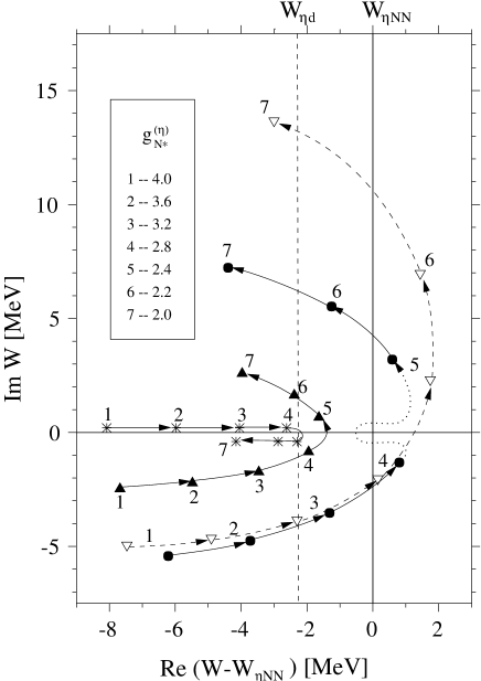
FIG. 8.: The pole trajectories of the $\eta NN$ scattering matrix for the $(J^{\pi};T)=(1^{-};0)$ state. Three trajectories correspond to the different choices of the $\pi NN^{*}$ coupling constant: $g_{N^{*}}^{(\pi)}$=0 (stars), $g_{N^{*}}^{(\pi)}$=1 (filled triangles), and $g_{N^{*}}^{(\pi)}$=1.5 (filled circles). The legend shows the values of the $\eta NN^{*}$ coupling constant $g_{N^{*}}^{(\eta)}$ being varied along the individual trajectory. The trajectory shown by the dashed curve is continued into the three-body sheet $\Pi_{3}$. The other trajectories pass into the two-body sheet $\Pi_{2}$ (see the text).

FIG. 9.: The pole trajectories of the $\eta NN$ scattering matrix for the $(J^{\pi};T)=(0^{-};1)$ state. Notation as in Fig. 8.

FIG. 10.: Elastic $\eta d$ cross section evaluated according to the approximate formula (41).

REFERENCES

- [1] R.E. Crien, et al., Phys. Rev. Lett. 60, 2595 (1988)
- [2] T. Ueda, Phys. Rev. Lett. 66, 297 (1991)
- [3] V.A. Tryasuchev, Phys. Atom. Nucl. 60, 186 (1997)
- [4] N.V. Shevchenko, V.B. Belyaev, S.A. Rakityansky, S.A. Sofianos, W. Sandhas, nucl-th/9908035
- [5] H. Garcilazo, M.T. Peña, nucl-th/0002056
- [6] S.A. Rakityansky, S.A. Sofianos, V.B. Belyaev, W. Sandhas, Phys. Rev. C 58, R2043 (1998)
- [7] A.M. Green, S. Wycech, Phys. Rev. C 55, R2167 (1997)
- [8] C. Wilkin, nucl-th/9810047
- [9] V. Metag, in Proceedings of the 8th International Conference on the Structure of Baryons, Bonn, 1998, edited by D.M. Menze and B. Metsch (World Scientific, Singapore 1999), p. 683
- [10] H. Cálen, et al., Phys. Rev. Lett. 80, 2069 (1998)
- [11] C. Bennhold, H. Tanabe, Nucl. Phys. A 530, 625 (1991)
- [12] V.A. Tryasuchev, A.I. Fiks, Phys. Atom. Nucl. 58, 1168 (1995)
- [13] L.J. Abu-Raddad, J. Piekarewicz, A.J. Sarty, M. Benmerrouche, Phys. Rev. C 57, 2053 (1998)
- [14] A. Fix, H. Arenhövel, Z. Phys. A 359, 427 (1997)
- [15] E.O. Alt, P. Grassberger, W. Sandhas, Nucl. Phys. B 2, 167 (1967)
- [16] Y. Yamaguchi, Phys. Rev. 95, 1628 (1954)
- [17] Particle Data Group, Review of Particle Physics, Eur. Phys. J. C 3, 1 (1998)
- [18] K. Möller, Yu.V. Orlov, Fiz. Elem. Chast. Atom. Yadra 20, 1341 (1989)
- [19] W. Glöckle, Phys. Rev. C 18, 564 (1978)
- [20] K. Möller, Czech. J. Phys. 32, 291 (1982)
- [21] E.A. Kolganova, A.K. Motovilov, Phys. Atom. Nucl. 60, 177 (1997), nucl-th/9602001
- [22] V.B. Belyaev, K. Möller, Z. Phys. A 279, 47 (1976)
- [23] A. Matsuyama, K. Yazaki, Nucl. Phys. A 534, 620 (1991)
- [24] J.R. Taylor, Scattering Theory (John Wiley Sons, New York 1972)
- [25] L.D. Landau, E.M. Lifshitz, Quantum Mechanics, Nonrelativistic Theory (Pergamon Press, Oxford, 1962)
- [26] H. Arenhövel, Nucl. Phys. A 247, 473 (1975)