Mean field theory for global binding systematics
Abstract
We review some possible improvements of mean field theory for application to nuclear binding systematics. Up to now, microscopic theory has been less successful than models starting from the liquid drop in describing accurately the global binding systematics. We believe that there are good prospects to develop a better global theory, using modern forms of energy density functionals and treating correlation energies systematically by the RPA.
I Introduction
An important goal of nuclear theory is to predict nuclear binding energies. While mean field theory offers the most fundamental basis to understand nuclear structure, paradoxically it has not been as successful than other approaches in making a global fit to nuclear binding energies. The most accurate theory of nuclear binding systematics [1] starts from the liquid drop model, and treats shell effects perturbatively. It fits the binding energies with an RMS deviation of 0.67 MeV, taking 15 free parameters and a similar number of fixed parameters to achieve the fit. No such systematic study with so many parameters has been attempted in a purely microscopic approach, but there are a number of partial studies beginning with the pioneering work of Vautherin and Brink[2] using an energy functional based on the Skyrme interaction. Noteworthy recent papers using Skyrme interactions are by Patyk et al. [3] and by Brown [4]. Patyk et al. find that Skyrme interactions taken from the literature give RMS errors greater than 2 MeV. This level is also found for the Gogny interaction, which unlike the Skyrme is finite range. Brown recently made a new Skyrme fit to closed shell nuclei, including radii and spectroscopic properties in the fitting [4]. He found an RMS deviation of 0.8 MeV for the 10 nuclei he considered, encouraging the hope that deviations below 1 MeV might be reached microscopically. Of course, open shell nuclei have significant correlation energies that must be included. We discuss how this might be done in Sect. 3 below. The other problem is the choice of energy density functional, and there may be reason to use other forms than the Skyrme or finite-range generalizations. This is discussed in the next section.
II New forms for the energy functional
Some perspective on the energy functional can be obtained from the analogous problem in condensed matter physics. Correlation effects are rather mild in the many-electron problem, and the mean field approach is very successful. The energy functional analogous to the Skyrme is called the local density approximation (LDA), and it is widely used to calculate structures of many-atom systems. Its accuracy for chemical purposes is inadequate, however. For example, in a comparison of different functionals Perdew et al. [5] noted that the LDA had a mean absolute error of 1.4 eV in a sample of small molecules with binding energies in the range 5-20 eV*** It should be mentioned, however, that the LDA energy functional is constructed ab initio without fitting binding data.. Two refinements of the energy functional, going beyond the LDA, make a dramatic improvement in the quality of agreement. The first refinement is to include a term in the energy functional that depends on the gradient of the density. Gradient terms are already present in the Skyrme interaction, but in the electron system improvement only appears with a nonlinear functional form of the gradient term,
| (1) |
The mean absolute error decreases by a factor of 4, to 0.35 eV, when this term is added†††Again, no free parameters are added with this term; the functional form and dependencies on and are constructed to simulate the nonlocality of the exchange.. The other improvement is to allow the functional to depend on the kinetic energy density and well as on the local density . This also is a familiar feature of the Skyrme interaction, but for the electron case the is combined with the dependence in eq. (1). The resulting mean absolute error is reduced by almost a factor of three to give a final mean absolute error of 0.13 eV.
The nuclear problem is different from the electronic is one important respect. In the electronic problem, much of the loss of accuracy is due to the exchange potential, which is intrinsically nonlocal but must be treated in a nearly local approximation for computational reasons. In contrast, in the nuclear problem the strong interaction is short-ranged, implying that the exchange is short-range as well and thus suited to local approximations. Nevertheless, it might be that more complicated functional forms such as eq. (1) could be useful in the nuclear problem. Indeed, this kind of generalization has be examined by Fayans [6]. He used such terms in an energy functional that was fit to 100 spherical nuclei. He obtained an RMS binding error of 1.2 MeV, a factor of two better than the Gogny or the published Skyrme functionals.
III Correlation energy
As mentioned earlier, in open shell nuclei the correlation energy associated with nearly degenerate configurations can be of the order of several MeV, so the single-configuration mean field approximation is not accurate enough for global energy systematics.
We believe that the following correlations should be considered
explicitly in the theory:
center-of-mass delocalization
quadrupole deformations
pairing.
These are the obvious correlations associated with symmetry breaking
in the mean field Hamiltonian.
Translational invariance is always broken in finite systems and rotational
invariance is often broken as well.
Pairing treated by BCS theory violates particle number conservation.
How important are these correlations to the energetics? For the center of mass, the correlation energy can be estimated in the harmonic oscillator model (but see below) as MeV. The resulting magnitude of several MeV is certainly much larger than the allowable error in a global mass theory. However, the energy varies very smoothly and one could question whether it needs to be treated explicitly as a correlation energy or whether its effect can be subsumed into the parameters of the mean-field energy functional. This might not be the case because the mean field functional determines most directly the leading terms in the liquid drop expansion, varying as and . One should not ask it to simulate a completely different -dependence. This argument, and some mean-field calculations to support, was given recently by Bender et al. [7].
The correlation energy associated with the deformations may be thought of as the energy gained by projecting the states of good angular momentum out of the deformed intrinsic state which contains many angular momenta. Its magnitude can be quite large on our accuracy scale of hundreds of keV. For example, the nucleus 20Ne has a Hartree-Fock ground state close in structure to the [8,0] SU(3) state of the harmonic oscillator. Combining probabilities of the different angular states with the energies of the states derived from the experimental spectrum, one can easily show that the energy gained by the projection is of the order of 4 MeV. A similar number was obtained recently in the projected mean-field calculations of 24Mg by ref. [8]. Thus this correlation energy should be included to accuracy of 10% or better to achieve the desired accuracy of the mass theory.
The situation with pairing is less severe. It is certainly necessary to including pairing in a theory of masses, just to get realistic odd-even mass differences, but the need to include correlation effects beyond the Hartree-Fock-Bogoliubov theory is less clear. With certain simplified pairing interactions the pairing Hamiltonian can be solved exactly, without making the BCS approximation [9]. The error in the BCS energy due to the number nonconservation is of the order of 0.5 MeV [10], Table 11.1. This might be significant in the global mass theory and we shall include it in our discussion.
There are many ways that correlation energies can be calculated. Most popular seems to be the obvious method in which the eigenstates of the symmetry are projected out of the mean-field wave function. If the energy minimization is carried out after the projection, this method is rather costly to use and probably not suitable for a global mass theory. For a global theory it is important that the method be simple computationally and also that it be systematic, applicable in principle to all possible mean field solutions. Particularly important is that it does not introduce a discontinuity when the mean field solution changes its character. In the systematic development of many-particle perturbation theory, the leading term beyond the mean-field approximation gave the correlation energy as an integral over the RPA excitation modes. In a finite system, the RPA correlation formula is given by[10, 11]
| (2) |
where is the (positive) frequency of the RPA phonon and is the matrix in the RPA equations. This approach was first proposed by Friedrich and Reinhard [12]. It seems to us that this formula is well-suited to the requirements we need for a systematic mass theory. We shall first argue that the formula is adequate in principle, and then take up the issue of computational feasibility. In the next section we summarize experience with simple model Hamiltonians that show that eq. (2) is more accurate than commonly used projection techniques, or is easier to calculate. In the section following we examine specific algorithms for calculating nuclear binding energies efficiently.
IV Experience from simple models
A Center-of-mass localization
The Hamiltonian of two particles interacting through a quadratic potential is solvable exactly and also has an analytic mean-field approximate solution. One might guess that the RPA correlation energy might give the correction exactly, because one can derive the RPA by considering quadratic approximations in a path integral formulation of the problem. This is indeed the case[13]. The RPA spectrum has two states, a zero-frequency mode and a finite frequency mode. Putting these frequencies in eq. (2), one finds that the correction to the mean-field energy is just what is needed to give the exact energy for the total, .
It is interesting to compare the RPA approach with other ways of dealing with correlation energies associated with broken symmetries. In the case of center-of-mass motion, a recipe that is often used is to subtract the expectation value of the center of mass operator from the mean field energy (e.g. in ref. [7]). With our Hamiltonian, this prescription gives
| (3) |
The total is not exact, although it is close to the exact energy, . This study shows that for this first kind of correlation the RPA formula provides a better method to calculate the associated energy.
B Deformations
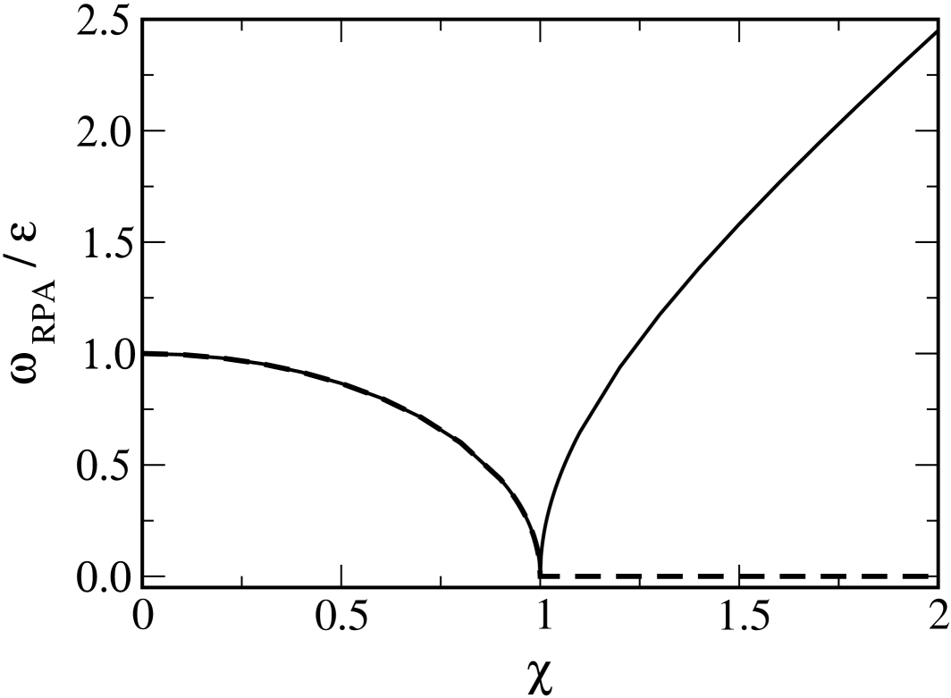
When the mean field solution is deformed, a continuous symmetry is broken. As in the above example, a signature of the broken continuous symmetry is a zero-frequency RPA mode. A model to test theories of the correlation energy should thus have a corresponding continuous symmetry. We constructed a model with those properties in ref. [13], making a generalization of the Lipkin model. In the original Lipkin model that has been studied for 40 years, one considers many distinguishable particles each of which can be in one of two states. For that model, the ground-state correlation was studied by Parikh and Rowe [14]. They compared various methods of treating the correlation energy, finding that the RPA formula worked best. In ref. [13], we extended the Lipkin model to a three-state wave function to get sufficient degrees of freedom for a continuously broken symmetry. The symmetry is imposed on the Hamiltonian by requiring it to be invariant under transformations within two of the three states. The two degenerate upper states could be thought of as the first excited states of a two-dimensional harmonic oscillator, thus allowing deformed wave functions in two dimensions. As expected, when the mean field solutions and its RPA excitations are calculated, ones sees a zero-frequency when the mean field solution is deformed. There is also another mode at finite frequency. In this case, the first mode corresponds to rotational motion perpendicular to the symmetry axis, while the second mode corresponds to the beta vibration. In the “spherical” phase, the RPA frequencies for the modes are identical and have finite frequency. Figure 1 shows the RPA frequencies as a function of for the particle number , where and are the strength of the interaction and the single-particle energy, respectively. One can clearly see the discontinuity at the critical point .
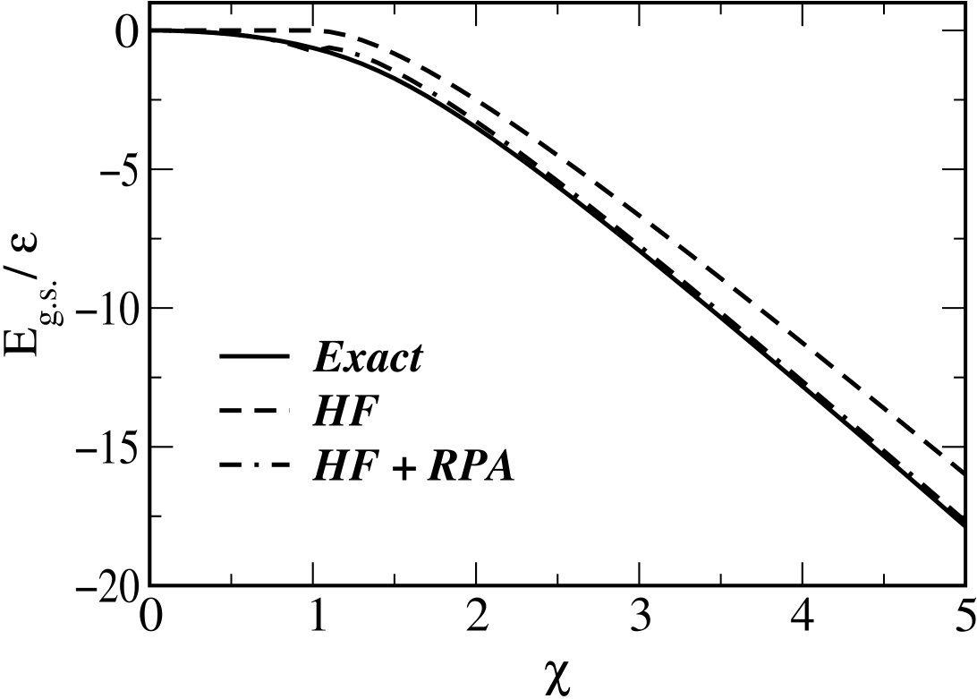
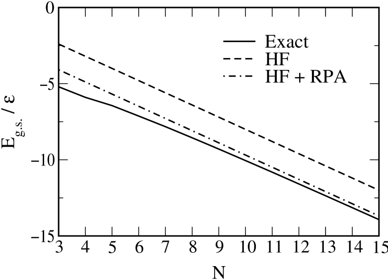
Figure 2 compares the ground state energy as a function of obtained by several methods. The number of particle is set to be 20. The solid line is the exact solution obtained by numerically diagonalizing the Hamiltonian. The dashed line is the ground state energy in the Hartree-Fock approximation. It considerably deviates from the exact solution through the entire range of shown in the figure. The dot-dashed line takes into account the RPA correlation energy in addition to the HF energy. Clearly the RPA significantly improves the results. The corresponding energy as a function of the number of particles is shown in Fig. 3. One sees that the RPA correlation energy is reliable for large , but may be problematic when there are only a few valence particles. That situation is further complicated by the pairing interaction, which may dominate the mean field solution for .
C Pairing
Pairing is the final example of a long-range correlation that significantly affects the energy. The mean field approach leads to the BCS theory, whose ground state has indefinite particle number. An early study by Bang and Krumlinde [15] showed that the RPA formula reproduces the exact correlation energy rather well in a schematic model. The RPA method has in fact been used in realistic models of deformed nuclei[16]. The RPA correlation in the normal phase was studied in ref. [17] using the self-consistent version of RPA.
Kyotoku et al. [18] derived the analytic solution for a model first proposed in ref. [19], fermions in a space of two nondegenerate j-shells interacting with a pairing Hamiltonian. They were able to solve the model exactly, and then compare the energy with several approximate methods to calculate the correlation corrections to the BCS energy. They found that the ground state energy in the BCS + quasi-particle RPA (QRPA) coincides with the exact solution at the leading order of an expansion in 1/, the number of particles in the system. None of the other methods obtained the correct coefficient of the leading order contribution. For example, the well-known method of Lipkin and Nogami [20] gave a result that is only correct in the limit of a strong pairing force (see Table I in ref. [18]).
In ref. [21], we specifically compared the RPA with the computationally attractive alternative methods, testing the behavior across shell closures and considering both even- and odd- systems. Taking as a test case the two-level problem with a level degeneracy of = 8 and a Fermi energy half way between the levels, the RPA was much superior to the Lipkin-Nogami method over most of the range of pairing strengths. This behavior is consistent with the result of ref.[18] as we discussed above. However, right at the phase transition point the two methods had comparable errors of opposite sign.
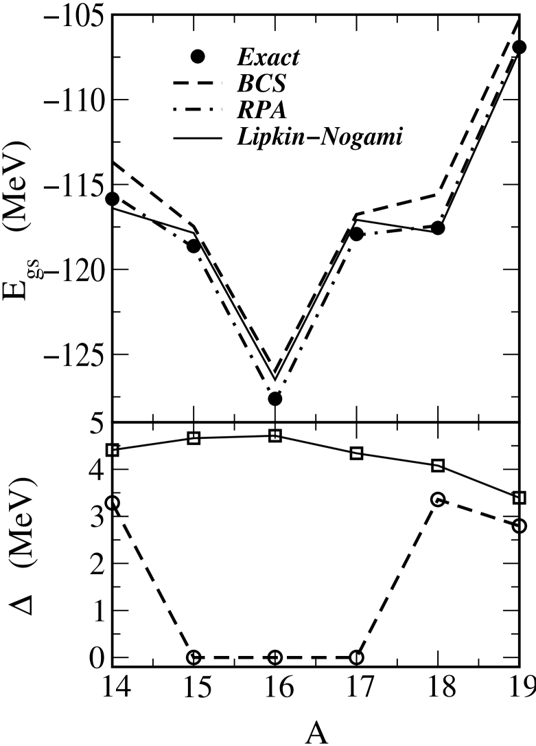
We therefore also looked at a more realistic situation, varying the particle number rather than the interaction strength . We consider the pairing energy in oxygen isotopes, taking the neutron 1p and 2s-1d shells as the lower and higher levels of the two-level model. The pair degeneracy thus reads and , for the lower and the upper levels, respectively. The number of particle in a system is given by for the AO nucleus. We assume that the energy difference between the two levels is given by and the pairing strength . The upper panel of Fig. 4 shows the ground state energy as a function of . In order to match with the experimental data for the 16O nucleus, we have added a constant MeV to the Hamiltonian for all the isotopes. The exact solutions are denoted by the filled circles. The deviation from the BCS approximation (the dashed line) is around 2 MeV for even systems and it is around 1.2 MeV for odd systems. This value varies within about 0.5 MeV along the isotopes and shows relatively strong dependence. One can notice that the RPA approach (the dot-dashed line) reproduces quite well the exact solutions. In contrast, the Lipkin-Nogami approach (the thin solid line) is much less satisfactory and shows a different dependence from the exact results. The pairing gap in the BCS approximation and in the Lipkin-Nogami method is shown separately in the lower panel of Fig. 4. For the Lipkin-Nogami method, we show , which are to be compared with experimental data [20]. The closed shell nucleus 16O and its neighbor nuclei 15,17O have a zero pairing gap in the BCS approximation, and the Lipkin-Nogami method does not work well for these nuclei. On the other hand, the RPA approach reproduces the correct dependence of the binding energy. Evidently, the RPA formula provides a better method to compute correlation energies than the Lipkin-Nogami method, especially for shell closures.
V Is RPA computationally feasible?
We now discuss the practicality of using eq. (2) to calculate the correlation energy. In general, the RPA is computationally more demanding than the mean field minimization for the ground state by an order of magnitude or more. One must diagonalize an RPA matrix whose dimension is , where is the number of particle-hole configurations. This number can be huge if one is interested in deformed nuclei or heavy spherical nuclei. A widely used way around this is to take a residual interaction has a separable form. Then the matrix equation to be solved has the dimension of the rank of the separable interaction; with a single term it is just the well-known algebraic dispersion relation.
Given a separable interaction, there are several efficient ways to the RPA correlation energy (2) without explicitly calculating all the roots of the dispersion relation. One method was recently proposed by Dönau et al.[22] and also by Shimizu et al. [23]. Instead of directly calculating the RPA correlation energy according to eq. (2), one carries out an integration of a function which depends on a free response function and its first derivative in a complex energy plane. An advantage of this method is that one can choose the integration path so that the integrand is smooth enough and thus the mesh of the numerical integration along such path can be much larger than the actual energy intervals of RPA solutions . This method is useful particularly when a separable interaction is used so that the free response function and its first derivative are analytically evaluated.
Alternatively, one can also use the Lanczos-type method proposed in ref. [24] to evaluate the RPA correlation energy. As we show below, this method quickly converges when the interaction is separable. The idea is to define at the outset a characteristic operator associated with each kind of correlation. That operator applied to the mean-field ground state gives an excited state, which is taken as the the first vector in a space built up by applications of the Hamiltonian to existing states. Eq. (2) is then evaluated in the restricted spaces, and the method would be computational feasible if the convergence is rapid enough.
Suppose and matrices in the RPA equation are given by
| (4) | |||||
| (5) |
where and label particle-hole configurations and is normalized as . For such an interaction, the collective operator can be chosen as . Notice that is an eigen-vector of the matrix with eigen-value and also that for any vector which is orthogonal to . Starting from the initial vectors and , the Lanczos manipulation [24] transforms the and matrices into the form of
| (6) |
The Lanczos basis for backward scattering amplitude remain all zero in the manipulation, and thus the transformed matrix has only one element which is not equal to zero. This is not in general the case for non-separable interaction. Note that the matrix measures the degree of correlation in the transformed space. Since it has a very simple form, the correlation energy evaluated in the restricted space converges very rapidly.
We have tested the method with RPA matrices given by eq. (5) with . The method works very well when there is a gap in the particle-hole spectrum. For example, taking a model with =20 particle-hole states and other parameters , , and , the RPA spectrum has a collective state at . The correlation energy from eq. (2) with all eigenvalues, is . The single-state approximation starting from the state is only off by 20%. The two-state approximation has an accuracy of 1%. The calculational effort to get this numbers is essentially that of three applications of the Hamiltonian to the ground-state single-particle wave function, much less than the effort to get the converged wave functions in the Hartree-Fock minimization. See Table I.
From our point of view, the problem is then to define a reliable separable interaction that can be used globally in RPA calculations. For particle-hole residual interactions, there have been proposed a few possible ways based on the self-consistency argument to construct a separable interaction [25, 26, 27, 28, 29]. The basic argument is that the collective motions primarily result in the displacement of the nuclear surface; thus the transition potential is can be generated by displacing the self-consistency potential associated with the ground state density. In equations, the transition density has a form locally given by the gradient of the static density, and the transition potential is the corresponding gradient of the static potential:
| (8) | |||||
where is an angle given the direction to an element of the nuclear surface. The separable residual interaction then has the shape of eq. (8) and the required magnitude to satisfied eq. (8). Thus
| (9) |
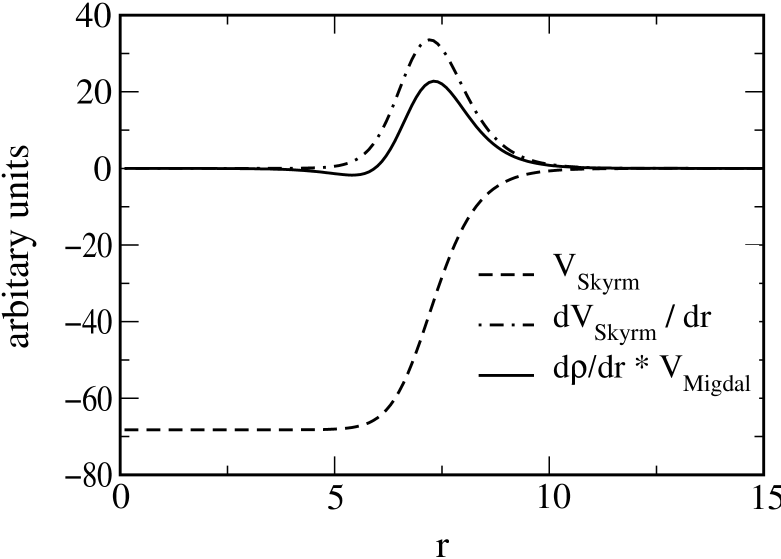
It is amusing to compare the above self-consistent definition with the microscopic particle-hole interaction proposed by Migdal [30]. For the above transition density, his transition potential would be given by
| (10) |
The two transition potentials for 208Pb are compared in Fig. 5. We generate the static potential using the velocity-independent part of the Skyrme interaction with SIII parametrisation and we use a Fermi distribution for a static density . The parameters of the Migdal interaction are given in ref. [31]. We see both the transition potentials have a similar surface-peaked radial dependence.
The above self-consistency argument can be applied very easily to the translation mode, where for translations in the -direction. For the rotational degrees of freedom, we would use the displacement fields associated with the 5 components of the quadrupole operator, i.e. . Note that the RPA correlations are to be evaluated for spherical as well as deformed nuclei; a major point of the approach is that the theory applies to all cases.
It is not so simple to construct a global, separable pairing interaction. The commonly used forms for the pairing interaction give divergent results without a cutoff in space of states included in the BCS calculation. Here we propose a non-local surface-peaked separable form,
| (11) |
The pairing matrix element of this interaction are to be evaluated as
| (12) |
This form is inspired by recent observations that the pairing is essentially a surface phenomenon [32, 33, 34]. A similar surface-peaked separable interaction was used for the particle-hole channel in ref. [35]. We have tested the surface-peaked separable pairing interactions (11) by comparing it with the density-dependent delta interaction proposed in ref. [36]. The problem of the cutoff is much less severe with this interaction than with a contact interaction, because the smoothness of cuts off the radial integrals. Our preliminary calculations show that the separable pairing interaction can reproduce results of the density-dependent pairing interaction reasonably well once the strength is adjusted. For the purpose of the global binding systematics, the -dependence of the strength has yet to be sorted out.
VI Summary
Our goal is to develop a better microscopic theory for the nuclear binding systematics. In this paper, we argued that the RPA approach provides a promising and computationally tractable way to include correlation effects in a global model, going beyond the mean-field approximation. We have shown that the HF + RPA approach works indeed well using simple Hamiltonian models for correlation associated with broken mean-field symmetries, namely the center-of-mass localization, rotation, and pairing. The RPA equation can be easily solved for a separable residual interaction. For example, the Lanczos method is quite efficient to solve the RPA equation for a separable interaction. This contrasts to other popular computational methods such as the generator coordinate method and the variation-with-projection method, which are rather complicated to apply. A work is now in progress to tackle the nuclear masses using the HF+RPA approach discussed in this paper.
Acknowledgment
We thank P.-G. Reinhard, W. Nazarewicz, B.A. Brown, and A. Bulgac for discussions. This work was supported by the U.S. Department of Energy under Grant no. DE-FG03-00-ER41132.
REFERENCES
- [1] P. Möller, J.R. Nix, W.D. Myers, W.J. Swiatecki, Atomic Data and Nuclear Data Tables 59, 185 (1995).
- [2] D. Vautherin and D.M. Brink, Phys. Rev. C5, 626 (1972).
- [3] Z. Patyk, A. Baran, J.F. Berger, J. Decharge, J. Dobaczewski, P. Ring, and A. Sobiczewski, Phys. Rev. C59, 704 (1999).
- [4] B.A. Brown, Phys. Rev. C58, 220 (1998).
- [5] J.P. Perdew, K. Burke, and M. Ernzerhof, Phys. Rev. Lett. 77, 3865 (1996); J.P. Perdew, S. Kurth, A. Zupan, and P. Blaha, Phys. Rev. Lett. 82, 2544 (1999).
- [6] S.A. Fayans, JETP Letters 68, 169 (1998).
- [7] M. Bender, K. Rutz, P.-G. Reinhard, and J.A. Maruhn, Euro. Phys. J. A7, 467 (2000).
- [8] A. Valor, P.-H. Heenen, and P. Bonche, Nucl. Phys. A671, 145 (2000).
- [9] R.W. Richardson and N. Sherman, Nucl. Phys. 52 221 (1964).
- [10] P. Ring and P. Schuck, The Nuclear Many Body Problem (Springer-Verlag, New York, 1980).
- [11] D.J. Rowe, Phys. Rev. 175, 1283 (1968).
- [12] J. Friedrich and P.-G. Reinhard, Phys. Rev. C33, 335 (1986).
- [13] K. Hagino and G.F. Bertsch, Phys. Rev. C61, 024307 (2000).
- [14] J.C. Parikh and D.J. Rowe, Phys. Rev. 175, 1293 (1968).
- [15] J. Bang and J. Krumlinde, Nucl. Phys. A141 (1970) 18.
- [16] Y.R. Shimizu, J.D. Garrett, R.A. Broglia, M. Gallardo, and E. Vigezzi, Rev. Mod. Phys. 61 (1989) 131.
- [17] J. Dukelsky, G. Röpke, and P. Schuck, Nucl. Phys. A628 (1998) 17; J. Dukelsky and P. Schuck, Phys. Lett. B464, 164 (1999).
- [18] M. Kyotoku, C.L. Lima, and Hsi-Tseng Chen, Phys. Rev. C53, 2243 (1996).
- [19] J. Högaasen-Feldman, Nucl. Phys. 28 (1961) 258.
- [20] H.J. Lipkin, Ann. Phys. (N.Y.) 9 (1960) 272; Y. Nogami, Phys. Rev. 134 (1964) B313; H.C. Pradhan, Y. Nogami, and J. Law, Nucl. Phys. A201 (1973) 357.
- [21] K. Hagino and G.F. Bertsch, nucl-th/0003016, Nucl. Phys. A, in press.
- [22] F. Dönau, D. Almehed, and R.G. Nazmitdinov, Phys. Rev. Lett. 83 (1999) 280.
- [23] Y.R. Shimizu, P. Donati, and R.A. Broglia, nucl-th/9911039.
- [24] C.W. Johnson, G.F. Bertsch, and W.D. Hazelton, Comp. Phys. Comm. 120 (1999) 155.
- [25] A. Bohr and B.R. Mottelson, Nuclear Structure (Benjamin, New York, 1975), vol. 2.
- [26] J. Babst and P.-G. Reinhard, Z. Phys. D42, 209 (1997).
- [27] V.O. Nesterenko, W. Kleinig, V.V. Gudkov, N. Lo Iudice, and J. Kvasil, Phys. Rev. A56, 607 (1997).
- [28] V.O. Nesterenko, W. Kleinig, V.V. Gudkov, and J. Kvasil, Phys. Rev. C53, 1632 (1996).
- [29] T. Suzuki and H. Sagawa, Prog. Theo. Phys. 65, 565 (1981).
- [30] A.B. Migdal, Theory of Finite Fermi Systems and Applications to Atomic Nuclei, (Wiley Interscience, New York, 1967).
- [31] P. Ring and J. Speth, Nucl. Phys. A235 (1974) 315.
- [32] F. Barranco, R.A. Broglia, G. Gori, E. Vigezzi, P.F. Bortignon, and J. Terasaki, Phys. Rev. Lett. 83, 2147 (1999).
- [33] M. Baldo, U. Lombardo, E. Saperstein, and M. Zverev, Phys. Lett. B459, 437 (1999).
- [34] M. Farine and P. Schuck, Phys. Lett. B459, 444 (1999).
- [35] Y. Alhassid, G.F. Bertsch, D.J. Dean, and S.E. Koonin, Phys. Rev. Lett. 77, 1444 (1996).
- [36] G.F. Bertsch and H. Esbensen, Ann. Phys. (N.Y.) 209, 327 (1991); H. Esbensen, G.F. Bertsch, and K. Hencken, Phys. Rev. C56, 3054 (1997).
| iteration number | ||
|---|---|---|
| 1 | 0.3326 | |
| 2 | 0.1539 | |
| 3 | 0.1454 | |
| exact | 0.1451 |