Dense Nuclear Matter:
Landau Fermi-Liquid Theory
and
Chiral Lagrangian with Scaling

Abstract

The relation between the effective chiral Lagrangian whose parameters scale according to Brown and Rho scaling(“BR scaling”) and Landau Fermi-liquid theory for hadronic matter is discussed in order to make a basis to describe the fluctuations under the extreme condition relevant to neutron stars. It is suggested that BR scaling gives the background around which the fluctuations are weak. A simple model with BR-scaled parameters is constructed and reproduces the properties of the nuclear ground state at normal nuclear matter density successfully. It shows that the tree level in the model Lagrangian is enough to describe the fluctuations around BR-scaled background. The model Lagrangian is consistent thermodynamically and reproduces relativistic Landau Fermi-liquid properties. Such points are important for dealing with hadronic matter under extreme condition. On the other hand it is shown that the vector current obtained from the chiral Lagrangian is the same as that obtained from Landau-Migdal approach. We can determine the Landau parameter in terms of BR-scaled parameter. However these two approaches provide different results, when applied to the axial charge. The numerical difference is small. It shows that the axial response is not included properly in the Landau-Migdal approach.

1 Introduction

Although QCD which deals with quarks and gluons is believed to be the fundamental theory for strong interactions, it is generally accepted that the appropriate theory at very low energy is the effective quantum field theory which incorporates the observed degrees of freedom in low-energy nuclear process, i.e., pions, nucleons and other low-mass hadrons [1, 2, 3, 4, 5, 6, 7]. The effective Lagrangian in matter-free or dilute space is governed by QCD symmetries with its parameters to be determined from experiments in free space. The energy scale of the experiments in which one is interested determines which hadrons play an important role in the theory. For example, it is shown [7] that one can integrate out even the pions for the two nucleon systems at very low energy. According to the results of [7], the deuteron and low-energy nucleon-nucleon scattering properties can be described very accurately by an effective theory given in terms of the nuclonic degrees of freedom only with a cutoff around the natural scale of the theory which for low energy is the pion mass.

Since there is currently growing interplay between the physics of hadrons and the physics of compact objects in astrophysics through the properties of hot and dense environments, we want to extend such successful strategy of effective field theories to a dense medium. First of all, our main goal is to understand the properties of dense hadronic medium which can be tested in various heavy ion collisions. Recent dilepton experiments (CERES and HELIOS-3) gave us very important information on the properties of hadrons in dense medium, which we will detail later. Understanding the properties of dense hadronic medium through heavy ion collision experiments is essential for understanding the properties of neutron stars which are believed to be formed in the center of supernovae at the time of explosions. Especially the determination of the maximum neutron star mass is one of the most important issues in astrophysics in explaining controversies between the observations and theoretical estimations, and it will give some hints for the detectibility of the gravitational wave detectors. A dense matter makes the probed energy scale larger than that in free space. Therefore we have to introduce more massive degrees of freedom which are usually vector meson and/or higher order operators in the nucleon fields. We must also consider a new energy scale, Fermi energy of nucleons in bound system.

The standard strategy to attack the dense hadronic matter is to obtain the ground state of matter and compute the excitations around it, based on an effective Lagrangian whose parameters are obtained in free space. Although such an approach can give satisfactory results with a sufficient number of parameters, it is not obvious whether we can extend the results for the different density. When the extension does not work, we usually face with very complicated loop diagrams which may lead to the impasse.

Another strategy is to start from the in-medium Lagrangian which is built on the reasonable assumptions, instead of deriving the hadronic matter properties from the matter-free effective Lagrangian defined in free space. In this approach one regards its mean field solution as a solution of the Wilsonian effective action in which the high energy modes are integrated out into the coefficient. We can compare it with the well-known Landau Fermi-liquid theory, which works at low energy excitation in strongly correlated Fermi system. Landau Fermi-liquid theory is described by quasiparticles, which are the low energy excitations in Fermi liquid, and their interactions under the assumption of one-to-one correspondence between the quasiparticle in the liquid and the particle in a non-interacting gas. It is a fixed point theory [8, 9] under Wilsonian renormalization to the Fermi surface [10] with $\Lambda/k_{F}\rightarrow 0$ if Bardeen-Cooper-Schrieffer(BCS) instability does not exist, where $\Lambda$ is the cutoff of the theory relative to the Fermi surface and $k_{F}$ is Fermi momentum. Since the result after the repeated renormalization does not depend on $k_{F}$, the argument for Fermi liquid holds as long as there is no phase transition. A famous example of such a Lagrangian is Walecka model. Its extension and justification were studied recently by Furnstahl et al. [11, 12, 13]. Their Lagrangian is constrainted by QCD symmetry and by Georgi’s naturalness condition and the coupling constants in it are tuned in order to describe nuclear ground state. Bulk properties of nuclei are described by it very successfully. But it is somewhat unclear to know how to approach the fluctuation on the ground state.

In this review we will approach the nuclear matter in a different way. We wish to apply the strategy of the effective field theory to the in-medium theory. We assume that the in-medium effective Lagrangian has the same structure as in free space according to the symmetry constraint of the fundamental theory QCD but that its parameters are modified in medium. It means that the effect of embedding a hadron in matter appears mainly in the change of the “vacuum,” i.e., quark and gluon condensate in QCD variables and the parameters in an effective theory. In this strategy the density-dependent parameters include many-body correlations.

Brown-Rho(BR) scaling [14] is one specific way to define such in-medium parameters. Brown-Rho scaling is the scaling of the dynamically generated masses of hadrons which consist of chiral quarks, i.e., $u$ and $d$ quarks. Brown and Rho phrased the scaling with the large $N_{c}$ Lagrangian, i.e., Skyrmion, under the assumption that the chiral symmetry and the scale symmetry of QCD are relevant. Their Lagrangian is implemented with scale anomaly of QCD, too. The masses and pion decay constant of this QCD effective theory scale universally:

$$\Phi(\rho)\approx\frac{f^{\star}_{\pi}(\rho)}{f_{\pi}}\approx\frac{m_{v}^{\star}(\rho)}{m_{v}}\approx\frac{m^{\star}_{\sigma}(\rho)}{m_{\sigma}}\approx\frac{M^{\star}(\rho)}{M}.$$ (1)

The star represents in-medium quantities here. $v$ is vector meson degree of freedom and $s$ an isoscalar scalar meson which has a mass $\sim$ 500 MeV in nuclear matter. $M$ represents a free nucleon mass and $M^{\star}$ a scaled nucleon mass which is somewhat different from the Landau effective mass discussed in Section 6.1.

It is known that BR scaling describes that the light-quark vector meson property in the extreme condition very successfully. One can make the extreme condition through relativistic heavy ion collisions. Specially the dileptons provide a good probe of the earlier dense and hot stage of relativistic heavy ion collision since the interaction of leptons is not subject to the strong interactions of the final state. CERES(Cherenkov Ring Electron Spectrometer) collaboration observed in heavy ion collision (S$+$Au) that the dilepton production with invariant masses from 250 MeV to about 500 MeV is enhanced much more than the predicted from the superposition of $pp$ collision [15]. And HELIOS-3(CERN Super Proton Synchrotron detector) [16] also observed the dilepton enhancement in S$+$W. It is shown by Li, Ko, and Brown [17] that a chiral Lagrangian with BR-scaled meson masses describes most economically and beautifully the enhancement, which is found to come from the dropping vector meson masses in dense matter. Furthermore the excitation into the kaonic direction above the given ground state seems to describe the properties of kaons in medium [18, 19] with scaled parameters [20].

Since BR scaling gives the universal scaling mass relation among hadrons, it must work for the baryon properties in medium. In recent works [21, 22, 23, 24, 25] it has been discussed how the BR scaling, which is applied to meson properties successfully, can be applied to the baryon property in dense medium and how it can be extrapolated to a hadronic matter under extreme conditions from the known normal nuclear matter. The construction of such bridges will be necessary to understand the various phenomena in relativistic heavy ion collisions and in compact stars in the universe. For those purposes we develop arguments for mapping the effective chiral Lagrangian whose parameters are governed by BR scaling to Landau Fermi-liquid theory. We will relate the meson mass scaling with baryon mass scaling and also relate matter properties with BR scaling parameter, which implies the vacuum structure characterized by quark condensate, via Landau parameter. Fermi liquid theory may work up to chiral phase transition, though the relevant degrees of freedom are changed to quasiquarks from quasihadrons.

In this review we approach the aim in two ways. The first is to obtain the ground state with BR scaling. How the Fermi surface is obtained in BR scaling framework is not yet understood clearly. So people usually assume that the ground state of hadronic matter is determined by the conventional matter from a standard many-body theory and use density-dependent effective chiral Lagrangians to compute mesonic fluctuations above the ground state. Though various fluctuation phenomena can be described successfully in this way, such a treatment gives no constraints for consistency between the excitations and the ground state. Though BR scaling is applied very successfully to describe meson properties in medium [17, 26], the way to deal with the matter properties is disconnected from BR scaling. Such a procedure is not satisfactory in going to the higher density region from the normal nuclear matter density. We can take the kaon condensation in neutron star as an example. In dealing with it, we come across a change of the ground state from that of a non-strange matter to a strange matter. The works up to date [27, 28] treated $KN$ interaction and the ground state separately. This is not satisfactory. Ground state properties might effect the condensation. For example, the effect of the four-Fermi interactions which play an important role in determining ground state, suppresses a pion condensation [29]. So we must deal with the whole bulk involving the ground state and excitations on top of it on the same footing. We assume that the ground state is given by the same effective Lagrangian that is supposed to include higher order corrections as the mean field of the BR-scaled chiral Lagrangian. We want to make an initial step for dealing with the ground state and the fluctuation on top of it on the same basis. We bridge these two properties by constructing a simple model whose parameters scale in the manner of BR and which describes nuclear matter properties well. It is shown that the model can be mapped to Landau Fermi-liquid theory.

The next step to achieve our aim is to identify the parameters of the BR-scaled effective Lagrangian with the fixed point quantities in Landau Fermi-liquid theory, given a hadronic matter with a Fermi surface. With this identification, certain mean field quantities of heavy meson (e.g. $\rho$, $\omega$) can be related to BR scaling through the Landau parameters. We show how such arguments work for the electromagnetic currents in nuclear matter. We can link a set of BR-scaled parameters at nuclear matter density with the orbital gyromagnetic ratio in terms of the Landau parameter $F_{1}^{\omega}$ which comes from integrated-out isoscalar vector degree of freedom in the effective Lagrangian. Then we will try to derive the corresponding formulas for the axial current in a similar way.

This review is organized as follows. In Section 2 Landau Fermi-liquid theory and its interpretation in terms of renormalization group language are summarized briefly. And we show how thermodynamic observables are related to the relativistic Landau parameters. In Section 3 the strategy of an effective field theory and how it is applied to a dense matter are explained. We proceed to discuss how nuclear matter described by an in-medium effective Lagrangian can be identified with Landau Fermi liquid. The model of Furnstahl, Serot and Tang [11] (referred to FTS1) which imposes the symmetries of QCD is examined as an example of the application of a general strategy of an effective chiral theory to a medium. In Section 4 Brown-Rho scaling is derived with QCD-oriented effective Lagrangian. A model where BR scaling governs the parameters of a chiral Lagrangian and determines the background at a given density is constructed in Section 5 in order to describe in weak coupling the same physics as FTS1 which has strong coupling in the form of a large anomalous dimension of a dilaton. It describes well normal nuclear matter properties and has thermodynamic consistency and Fermi-liquid structure needed for the extrapolation to higher density region. In Section 6 vector current and axial charge transition matrix elements for a nucleon above the given Fermi sea in Landau-Migdal theory and in chiral effective Lagrangian are calculated and compared. A summary and comments on some unsolved problems are given in Section 7 and Section 8 respectively. Appendix A shows how sensitive the equation of state is to the many-body correlation parameters for $\rho>\rho_{0}$. Appendix B shows how to compute relativistically the pionic contribution to Landau parameter $F_{1}$ by means of Fierz transformation. And the vector-mesonic contribution to $F_{1}$ and to electromagnetic convection current is calculated in Appendix C relativistically with random phase approximation.

2 Landau Fermi-liquid theory

We discuss briefly Landau Fermi-liquid theory in this section, before presenting the relation between the chiral effective theory for nuclear matter and Landau Fermi-liquid theory. A mini-primer on Landau Fermi-liquid theory is given in the first subsection to define the quantities involved. In the second subsection, it is discussed that Landau Fermi-liquid theory is considered as an effective theory and is shown to be a fixed point theory in renormalization group(RG) language. And we will show how the thermodynamic quantities are related to relativistic Landau parameters in Section 2.3.

2.1 A mini-primer

Landau’s Fermi-liquid theory is a semi-phenomenological approach to strongly interacting normal Fermi systems at small excitation energies. The elementary excitations of the Fermi-liquid, which correspond to single particle degrees of freedom of the Fermi gas, are called quasiparticles in Landau Fermi-liquid theory. It is assumed that a one-to-one correspondence exists between the low-energy excitations of the Fermi liquid near Fermi surface, i.e., quasiparticles, and those of a non-interacting Fermi gas. A quasiparticle state of the interacting liquid is obtained by turning on the interaction adiabatically at the corresponding state of non-interacting Fermi gas. The quasiparticle properties, e.g. the mass, in general differ from those of free particles due to interaction effects. In addition there is a residual quasiparticle interaction, which is parameterized in terms of the so called Landau parameters.

The adiabatic process described above is possible in the vicinity of the Fermi surface only. Let us see the Fermi liquid at $T=0$. Since Pauli exclusion principle makes the states below the Fermi surface filled, quasiparticle with energy $\varepsilon$ loses energy less than $\varepsilon-\varepsilon_{F}$ when colliding the background particles. It means that the quasiparticles which can interact with the quasiparticle are those with an energy within $|\varepsilon-\varepsilon_{F}|$ of the Fermi surface. And the final state momenta are also restricted by $\varepsilon^{\prime}<\varepsilon$. Pauli exclusion principle and the corresponding rarity of final states make the quasiparticle life time proportional to $|\varepsilon-\varepsilon_{F}|^{-2}$ at $T=0$ case.

Fermi-liquid theory is a prototype effective theory, which works because there is a separation of scales. The theory is applicable to low-energy phenomena, while the parameters of the theory are determined by interactions at higher energies. The separation of scales is due to the Pauli principle and the finite range of the interaction. Pauli principle makes the low energy quasiparticle physics possible near the Fermi surface and the finite range of interaction makes a few quasiparticles around Fermi surface, who appear by the small change of the energy in low energy physics, form a gas. Fermi-liquid theory has proven very useful [30] for describing the properties of e.g. liquid ³He and provides a theoretical foundation for the nuclear shell model [31] as well as nuclear dynamics of low-energy excitations [32, 33].

The interaction between two quasiparticles ${\mbox{\boldmath$p$}_{1}}$ and ${\mbox{\boldmath$p$}_{2}}$ at the Fermi surface of symmetric nuclear matter can be written in terms of a few spin and isospin invariants [34]

$${f}_{\mbox{\boldmath$p$}_{1}\sigma_{1}\tau_{1},\mbox{\boldmath$p$}_{2}\sigma_{2}\tau_{2}} = \frac{1}{N(0)}\left[F(\cos\theta_{12})+F^{\prime}(\cos\theta_{12})\mbox{\boldmath$\tau$}_{1}\cdot\mbox{\boldmath$\tau$}_{2}+G(\cos\theta_{12})\mbox{\boldmath$\sigma$}_{1}\cdot\mbox{\boldmath$\sigma$}_{2}\phantom{\frac{\mbox{\boldmath$q$}^{\,2}}{k_{F}^{2}}}\right.$$ (2)

$$+ \left.G^{\prime}(\cos\theta_{12})\mbox{\boldmath$\sigma$}_{1}\cdot\mbox{\boldmath$\sigma$}_{2}\mbox{\boldmath$\tau$}_{1}\cdot\mbox{\boldmath$\tau$}_{2}+\frac{\mbox{\boldmath$q$}^{\,2}}{k_{F}^{2}}H(\cos\theta_{12})S_{12}(\mbox{\boldmath$\hat{q}$})\right.$$

$$+ \left.\frac{\mbox{\boldmath$q$}^{\,2}}{k_{F}^{2}}H^{\prime}(\cos\theta_{12})S_{12}(\mbox{\boldmath$\hat{q}$})\mbox{\boldmath$\tau$}_{1}\cdot\mbox{\boldmath$\tau$}_{2}\right]$$

where $\theta_{12}$ is the angle between ${\mbox{\boldmath$p$}_{1}}$ and ${\mbox{\boldmath$p$}_{2}}$ and $N(0)=\frac{\gamma k_{F}^{2}}{(2\pi^{2})}\left(\frac{dp}{d\varepsilon}\right)_{F}$ is the density of states at the Fermi surface. In this review natural units where $\hbar=1$ are used. The spin and isospin degeneracy factor $\gamma$ is equal to 4 in symmetric nuclear matter. Furthermore, $\mbox{\boldmath$q$}=\mbox{\boldmath$p$}_{1}-\mbox{\boldmath$p$}_{2}$ and

$$S_{12}(\mbox{\boldmath$\hat{q}$})=3\mbox{\boldmath$\sigma$}_{1}\cdot\mbox{\boldmath$\hat{q}$}\mbox{\boldmath$\sigma$}_{2}\cdot\mbox{\boldmath$\hat{q}$}-\mbox{\boldmath$\sigma$}_{1}\cdot\mbox{\boldmath$\sigma$}_{2},$$ (3)

where $\mbox{\boldmath$\hat{q}$}=\mbox{\boldmath$q$}/|\mbox{\boldmath$q$}|$. The tensor interactions $H$ and $H^{\prime}$ turn out to be important for the axial charge [34] The functions $F,F^{\prime},\dots$ are expanded in Legendre polynomials,

$$F(\cos\theta_{12})=\sum_{\ell}F_{\ell}P_{\ell}(\cos\theta_{12}),$$ (4)

with analogous expansion for the spin- and isospin-dependent interactions. The energy of a quasiparticle with momentum $p=|{\mbox{\boldmath$p$}}|$, spin $\sigma$ and isospin $\tau$ is denoted by $\epsilon_{p,\sigma,\tau}$ and the corresponding quasiparticle number distribution by $n_{p,\sigma,\tau}$. From now on the spin and isospin indices $\sigma$ and $\tau$ will be omitted from the formulas to avoid overcrowding, except where needed to avoid ambiguities.

$$n_{p}(\mbox{\boldmath$r$},t) = n_{p}^{0}(\varepsilon^{0}_{p})+\delta n_{P}(\mbox{\boldmath$r$},t)$$ (5)

$$\varepsilon_{p}(\mbox{\boldmath$r$},t) = \varepsilon_{p}^{0}+\sum_{\sigma^{\prime},\tau^{\prime}}\int\frac{d^{3}p^{\prime}}{(2\pi)^{3}}f_{pp^{\prime}}\delta n_{p^{\prime}}(\mbox{\boldmath$r$},t)$$ (6)

where $\delta n_{p}(\mbox{\boldmath$r$},t)$ is the long wave length excitations from the ground state $n_{p}^{0}(\varepsilon^{0})$ in the vicinity of Fermi surface. The space and time dependence of the quantities will also be omitted, e.g., $\varepsilon\equiv\varepsilon({\mbox{\boldmath$r$}},t)$. The Landau effective mass and velocity of a quasiparticle on the Fermi surface is defined by

$$\left.\frac{d\varepsilon_{p}}{dp}\right|_{p=k_{F}}=\frac{k_{F}}{m_{L}^{\star}}\equiv v_{F}^{\star}.$$ (7)

We must note that the total current is not

$$\mbox{\boldmath$J$}_{locQP}=\sum_{\sigma,\tau}\int\frac{d^{3}p}{(2\pi)^{3}}\mbox{\boldmath$v$}_{F}^{\star}\delta n_{p}$$ (8)

in Landau Fermi-liquid theory. The quasiparticle distribution $n_{p}(\mbox{\boldmath$r$},t)$ obeys

$$\frac{\partial n_{p}}{\partial t}+\frac{d\mbox{\boldmath$r$}}{dt}\cdot\mbox{\boldmath$\nabla$}_{r}n_{p}+\frac{d\mbox{\boldmath$p$}}{dt}\cdot\mbox{\boldmath$\nabla$}_{p}n_{p}=0.$$ (9)

The key assumption of Landau Fermi-liquid kinetic theory is that $\varepsilon_{p}(\mbox{\boldmath$r$},t)$ plays the role of the quasiparticle Hamiltonian;

$$\frac{d\mbox{\boldmath$p$}}{dt} = -\mbox{\boldmath$\nabla$}_{r}\varepsilon_{p}$$ (10)

$$\frac{d\mbox{\boldmath$r$}}{dt} = \mbox{\boldmath$\nabla$}_{p}\varepsilon_{p}.$$ (11)

The kinetic equation is

$$\frac{\partial n_{p}}{\partial t}+\mbox{\boldmath$\nabla$}_{r}n_{p}\cdot\mbox{\boldmath$\nabla$}_{p}\varepsilon_{p}-\mbox{\boldmath$\nabla$}_{p}n_{p}\cdot\mbox{\boldmath$\nabla$}_{r}\varepsilon_{p}=I[n_{p^{\prime}}]$$ (12)

where $I[n_{p^{\prime}}]$ is an internal collision integral which represents the sudden change of quasiparticle momenta. We consider the system without external forces. Integrating over $p$, that cancels the effect of the internal collision under the assumption that the quasiparticle energy, momentum and number are locally conserved, (12) becomes (to order $\delta n_{p}(\mbox{\boldmath$r$},t)$), by integration by part,

$$\sum_{\sigma,\tau}\int\frac{d^{3}p}{(2\pi)^{3}}\frac{\partial\delta n_{p}}{\partial t}+\mbox{\boldmath$\nabla$}_{r}\cdot(n_{p}\mbox{\boldmath$\nabla$}_{p}\varepsilon_{p}) = \frac{\partial\delta\rho}{\partial t}+\sum_{\sigma,\tau}\mbox{\boldmath$\nabla$}_{r}\cdot\int\frac{d^{3}p}{(2\pi)^{3}}\delta n_{p}\mbox{\boldmath$\nabla$}_{p}\varepsilon_{p}+\delta\varepsilon_{p}\mbox{\boldmath$\nabla$}_{p}n_{p}^{0}$$ (13)

$$= 0$$

where $\delta\rho$ is the total particle (or quasiparticle) density fluctuation. We can easily see that the conserved current is

$$J = \sum_{\sigma,\tau}\int\frac{d^{3}p}{(2\pi)^{3}}n_{p}\mbox{\boldmath$\nabla$}_{p}\varepsilon_{p}$$ (14)

$$= \sum_{\sigma,\tau}\int\frac{d^{3}p}{(2\pi)^{3}}\mbox{\boldmath$v$}_{F}^{\star}\delta n_{p}^{loc}$$

with the excitation from the local equilibrium $n_{p}^{0}(\varepsilon(\mbox{\boldmath$r$},t))$;

$$n_{p}(\mbox{\boldmath$r$},t)=n_{p}^{0}(\varepsilon(\mbox{\boldmath$r$},t))+\delta n_{p}^{loc}(\mbox{\boldmath$r$},t).$$ (15)

Comparing (15) with (5) and (6), we obtain

$$\delta n_{p}^{loc}=\delta n_{p}+\frac{\partial n_{p}^{0}}{\partial\varepsilon}\sum_{\sigma^{\prime},\tau^{\prime}}\frac{d^{3}p^{\prime}}{(2\pi)^{3}}f_{pp^{\prime}}\delta n_{p}^{\prime}.$$ (16)

The modification $\mbox{\boldmath$J$}_{locQP}-\mbox{\boldmath$J$}$ can be interpreted as the effect of the return flow of the surrounding matter to the localized wave packet carrying $J$ and is called back-flow current.

2.2 Renormlization group approach

Landau Fermi-liquid theory was based on Landau’s reasonable intuition. After his work, his theory was derived and justified microscopically [35]. Recent development of Wilsonian RG method in medium [10] provides us a new understanding of Fermi liquid theory. Landau Fermi-liquid theory is a fixed point theory described by marginal coupling, i.e. ${\mathcal{F}}$, $m_{L}^{\star}$ [8]. In this section we will review the RG arguments for Fermi liquid theory.

To do this we consider a nonrelativistic system of spinless fermions whose Fermi surface is spherical characterized by $k_{F}$ for simplicity. Then non-interacting one particle Hamiltonian near Fermi surface is

$$H=\frac{\mbox{\boldmath$K$}^{2}}{2m}-\frac{k_{F}^{2}}{2m}\approx\frac{k}{m}k_{F}\equiv v_{F}k$$ (17)

with $k=|\mbox{\boldmath$K$}|-k_{F}$. The free fermion field action

$$S_{0}=\int_{\Lambda}\bar{\psi}(\omega k\Omega)(i\omega-vk)\psi(\omega k\Omega)$$ (18)

in momentum space where

$$\int_{\Lambda}:=\int\frac{d\Omega}{(2\pi)^{2}}\int_{-\Lambda}^{\Lambda}\frac{dk}{(2\pi)}\int_{-\infty}^{\infty}\frac{d\omega}{(2\pi)}.$$ (19)

$\bar{\psi}$ and $\psi$ are Grassmannian eigenvalue with fermion operator $\hat{\Psi}$; $\hat{\Psi}|\psi\rangle=\psi|\psi\rangle$ and $\langle\bar{\psi}|\hat{\Psi}^{\dagger}=\langle\bar{\psi}|\bar{\psi}$. Note that a shell of thickness $\Lambda$ on either side of the Fermi surface is taken for low energy physics as seen in Fig. 1.

Figure 1: Our interest lies in the spherical shell which is of the thickness of $\Lambda$ on either side of Fermi sphere. In RG transformation we eliminate the mode within the two thick-lined shells whose thickness is $d\Lambda$.

Pauli exclusion principle lets only small deviations from the Fermi surface, not from the origin, be important in low energy physics of fermion matter. This defines the starting point of an in-medium renormalization group procedure.

The first step for the renormalization is decimation; to integrate out the high energy mode whose momentum is larger than $\Lambda/s$ and to reduce the cutoff from $\Lambda$ to $\Lambda/s$. For example, the free action (18) becomes

$$S_{0}^{eff}=\int\frac{d\Omega}{(2\pi)^{2}}\int_{-\Lambda/s}^{\Lambda/s}\frac{dk}{(2\pi)}\int_{-\infty}^{\infty}\frac{d\omega}{(2\pi)}\bar{\psi}(\omega k\Omega)(i\omega-vk)\psi(\omega k\Omega).$$ (20)

Next we rescale the momenta in order to compare the old and the new;

$$(\omega,\mbox{\boldmath$k$})\rightarrow(s\omega,s\mbox{\boldmath$k$}).$$ (21)

The last step is to absorb the uninteresting multiplicative constant by

$$\psi\rightarrow s^{-3/2}\psi.$$ (22)

The RG transformation consists of these three steps. After such RG transformation, the free action (18) returns to the old. When a coupling is turned on, the coupling is called relevant if it increases after RG transformation. If it decreases, it is called irrelevant and if it remains fixed like the free action, it is called marginal.

Now let us turn on four-Fermi interaction. The appropriate action is

$$S = \int_{\Lambda}\bar{\psi}[i\omega-v_{F}^{\star}k]\psi+\delta\mu^{\star}\int_{\Lambda}\bar{\psi}\psi$$ (23)

$$+\frac{1}{2!2!}\int_{\Lambda_{4}}u(4,3,2,1)\bar{\psi}(4)\bar{\psi}(3)\psi(2)\psi(1)$$

where $(i)$ represents $(\omega_{i},k_{i},\Omega_{i})$ and

$$\int_{\Lambda_{4}}:=\prod_{i}\int\frac{d\Omega}{(2\pi)^{2}}\int_{-\Lambda}^{\Lambda}\frac{dk}{(2\pi)^{2}}\int_{-\infty}^{\infty}\frac{d\omega}{(2\pi)}\Theta(\Lambda-|\mbox{\boldmath$k$}_{4}|).$$ (24)

with a cutoff function for $k_{4}$, $\Theta(\Lambda-|\mbox{\boldmath$k$}_{4}|)$, which is needed to make all the momenta lie within the band of width $2\Lambda$ around the Fermi surface. Here $v_{F}^{\star}=k_{F}/m^{\star}$ and

$$m^{\star}=\frac{1}{Z(1+\frac{m}{k_{F}}\frac{\partial\Sigma}{\partial k})}$$ (25)

is the effective mass of the nucleon which will be equal to the Landau mass $m_{L}^{\star}$ as will be elaborated on later. $\Sigma(\omega,k)$ is self-energy and $1/Z=1+i\frac{\partial\Sigma}{\partial\omega}$. The effective mass arises because the eliminated mode contributes to $i\omega\bar{\psi}\psi$ and $k\bar{\psi}\psi$ differently. By defining $\psi^{\prime}=s^{-3/2}Z^{-1/2}\psi$ we fix the coefficient of $i\omega\bar{\psi}\psi$ and define the effective mass. The term with $\delta\mu^{\star}$ is a counter term added to assure that the Fermi momentum is fixed (that is, the density is fixed). What this term does is to cancel loop contributions involving the four-Fermi interaction to the nucleon self-energy (i.e., the tadpole) which contributes marginally so that the $v_{F}^{\star}$ is at the fixed point. Since other contributions which can be written as $-\Sigma\bar{\psi}\psi$ are irrelevant, $m$ moves to $m^{\star}$ in earlier stage of renormalization but becomes a fixed point characterized by some $m^{\star}$. This means that the counter term essentially assures that the effective mass $m^{\star}$ be at the fixed point. Without this procedure, the term quadratic in the fermion field would be “relevant” and hence would be unnatural [8].

Let us see the quartic coupling $u$ at tree level. The cutoff function $\Theta(\Lambda-|\mbox{\boldmath$k$}_{4}|)$ in (24) makes the coupling depend on angles on the Fermi surface. Since all the momenta are on the thin spherical shell near $k_{F}$, momentum conservation makes the new quartic coupling $u^{\prime}(\omega^{\prime},k^{\prime},\Omega^{\prime})$ decay after the RG transformation at tree level except for the two cases. One is that $\mbox{\boldmath$K$}_{3}$ and $\mbox{\boldmath$K$}_{4}$ are the rotation of $\mbox{\boldmath$K$}_{1}$ and $\mbox{\boldmath$K$}_{2}$ around the $\mbox{\boldmath$K$}_{1}+\mbox{\boldmath$K$}_{2}$ as seen in Fig. 2.

Figure 2: Momentum conservation and the physics near Fermi surface force the angle between $\mbox{\boldmath$K$}_{3}$ and $\mbox{\boldmath$K$}_{4}$ to be the same as that between $\mbox{\boldmath$K$}_{1}$ and $\mbox{\boldmath$K$}_{2}$ unless $\mbox{\boldmath$K$}_{2}=-\mbox{\boldmath$K$}_{1}$.

In that case, the opening angle $\cos^{-1}(\mbox{\boldmath$\hat{u}$}_{1}\cdot\mbox{\boldmath$\hat{u}$}_{2})$ is fixed where $\mbox{\boldmath$\hat{u}$}_{i}$ is a unit vector in the direction of $\mbox{\boldmath$K$}_{i}$. The other, so-called BCS coupling, is that $\mbox{\boldmath$\hat{u}$}_{1}=-\mbox{\boldmath$\hat{u}$}_{2}$ and $\mbox{\boldmath$\hat{u}$}_{3}=-\mbox{\boldmath$\hat{u}$}_{4}$. These cases are represented by functions;

$$u(\theta_{12}=\theta_{34}) = {\mathcal{F}}(\theta_{12},\vartheta)$$ (26)

$$u(\theta_{13}=\theta_{24}) = {\mathcal{V}}(\theta_{13})$$

where $\theta_{ij}=\mbox{\boldmath$\hat{u}$}_{i}\cdot\mbox{\boldmath$\hat{u}$}_{j}$ and $\vartheta$ is the angle between the planes containing $(\mbox{\boldmath$K$}_{1},\mbox{\boldmath$K$}_{2})$ and $(\mbox{\boldmath$K$}_{3},\mbox{\boldmath$K$}_{4})$ respectively. ${\mathcal{F}}$ and ${\mathcal{V}}$ are marginal at tree level.

Then the next question is how ${\mathcal{F}}$ and ${\mathcal{V}}$ evolve at one loop level. Figure 3 shows the one loop diagrams for the evolution.

Figure 3: One loop diagrams for the renormalization of the marginal quartic couplings ${\mathcal{F}}$ and ${\mathcal{V}}$.

Integrating out the momentum shell of thickness $d\Lambda$ at $k=\pm\Lambda$ and sending $\Lambda/k_{F}\rightarrow 0$, all the diagrams in Fig. 3 do not contribute to ${\mathcal{F}}$. So ${\mathcal{F}}$ is left marginal to the one loop order. In the case of ${\mathcal{V}}$, the third diagram in Fig. 3 makes a flow. When we expand ${\mathcal{V}}$ in terms of angular momentum eigenfunction, ${\mathcal{V}}$ becomes irrelevant only if all the ${\mathcal{V}}_{l}$’s are repulsive. However, if any ${\mathcal{V}}_{l}$ is attractive, it becomes relevant and causes BCS instability. We call it BCS channel. Since Landau theory assures that there is no phase transition for one-to-one correspondence between particles and quasiparticles, BCS channel destabilizes in Landau Fermi-liquid theory.

If we divide the angular part of the shell integration in the action (18) into the cells of size $\Delta\Omega\sim\Lambda/k_{F}$, the shell is split into $\sim k_{F}/\Lambda$ cells. By analogy with large $N$ theory each cell corresponds to one species, i.e., $N\sim k_{F}/\Lambda$. $1/N$ expansion tells that all higher loop corrections except for the bubbles of the first diagram in Fig. 3 are down by powers of $1/N=\Lambda/k_{F}$. And the contributions of bubbles of the first diagram survive but are irrelevant to the $\beta$ function. Only one loop contributions to $\beta$ function survive in the large $N$ limit. So the four-Fermi interactions in the phonon channel ${\mathcal{F}}$ are also at the fixed points in addition to the Fermi surface fixed point with the effective mass $m^{\star}$. Note that only forward scattering ${\mathcal{F}}(\vartheta=0)$ is important for responses to soft probes, since nonforward amplitudes in loop calculations are also suppressed by $1/N$. Six-Fermi and higher-Fermi interactions are irrelevant and contribute at most screening of the fixed-point constants. The Landau parameter $F$ can be identified with forward scattering $\gamma\frac{m^{\star}}{2\pi^{2}k_{F}}{\mathcal{F}}(\vartheta=0)$ easily [8]. We arrive at the Fermi-liquid fixed point theory in the absence of BCS interactions.

Chen, Fröhlich, and Seifert [9] obtain the same result in the $1/N$ expansion where their $N$ is taken to be $N\sim\lambda$ with $1/\lambda$ being the width of the effective wave vector space around the Fermi sea which can be considered as the ratio of the microscopic scale to the mesoscopic scale. More specifically if one rescales the four-Fermi interaction such that one defines the dimensionless constant $g\sim u_{0}/k_{F}^{2}$ where $u_{0}$ is the leading term (i.e., constant term) in the Taylor series of the quantity $u$ in (23), then the fermion wave function renormalization $Z$, the Fermi velocity $v_{F}$ and the constant $g$ are found not to flow up to order ${{\mathcal{O}}}(g^{2}/N)$. Thus in the large $N$ limit, the system flows to Landau fixed point theory to all orders of loop corrections. This result is correct provided there are no long-range interactions and if the BCS channel is turned off.

2.3 Relations for relativistic Fermi-liquid

In this section we briefly summarize the relations of physical properties of the relativistic Landau Fermi-liquid. The extension of Landau Fermi-liquid theory to relativistic region for high density matter is found in [36]. It should be pointed out that one can use all the standard Landau Fermi-liquid relations established below in our calculations once fixed point quantities are identified in the chiral Lagrangian.

2.3.1 Compression modulus and $F_{0}$

The density of states at Fermi surface is

$$N(0) = \left(\frac{\partial\rho}{\partial\varepsilon}\right)_{k_{F}}=\frac{\gamma k_{F}m_{L}^{\star}}{2\pi^{2}}.$$ (27)

Note that $m_{L}^{\star}=\sqrt{m_{N}^{2}+k_{F}^{2}}$ for relativistic non-interacting Fermi gas. $m_{L}^{\star}$ defined by (7) includes the kinetic energy for relativistic Fermi liquid. The chemical potential is defined by

$$\mu\equiv\frac{\partial{\mathcal{E}}}{\partial\rho}=\varepsilon_{F}$$ (28)

where ${\mathcal{E}}$ represents the energy per volume. Using (27) and (28) one can derive the relativistic relation between compression modulus which represents the change of volume with pressure and $F_{0}$ in the same way as the nonrelativistic one:

$$K = 9\rho\frac{\partial\mu}{\partial\rho}=9\rho\frac{\partial}{\partial\rho}\left(\varepsilon^{0}_{p}+\int d\tau^{\prime}f_{pp^{\prime}}n_{p^{\prime}}\right)$$ (29)

$$= \frac{3k_{F}^{2}}{m_{L}^{\star}}(1+F_{0})$$

Here $\rho$ is the baryon number density and $n_{p}$ is the Fermi distribution function for the state of momentum $p$.

2.3.2 Landau effective mass

In deriving the Landau mass formula, we shall compare the rest frame and the boosted frame with very small velocity $u$ and check Lorentz symmetry. Since $u\equiv|\mbox{\boldmath$u$}|$ is small we neglect the order of $u^{2}$ in the process of the derivation. (Note that $\gamma_{u}=(1-u^{2})^{-1/2}\approx 1$ in that order. )

Let us first derive the relativistic relation between the Landau effective mass and the velocity dependence of the quasiparticle interaction. When we add a particle (or equivalently quasiparticle) of momentum $p$ in the rest frame to the system, the energy and the momentum of the system increases by $p$ and $\varepsilon_{p}(0)$ respectively. In a moving frame with velocity $-\mbox{\boldmath$u$}$, the momentum and energy increase by

$$\mbox{\boldmath$p$}^{\prime} = \mbox{\boldmath$p$}-\mbox{\boldmath$\hat{u}$}(\mbox{\boldmath$\hat{u}$}\cdot\mbox{\boldmath$p$})(1-\gamma_{u})+\varepsilon_{p}(0)\mbox{\boldmath$u$}\gamma_{u}$$ (30)

$$\approx \mbox{\boldmath$p$}+\varepsilon_{p}(0)\mbox{\boldmath$u$}$$

$$\varepsilon_{p^{\prime}}(u) = (\varepsilon_{p}(0)+\mbox{\boldmath$p$}\cdot\mbox{\boldmath$u$})\gamma_{u}$$ (31)

$$\approx \varepsilon_{p}(0)+\mbox{\boldmath$p$}\cdot\mbox{\boldmath$u$}.$$

From $\varepsilon_{p}(u)$. (30) and (31), we have

$$\varepsilon_{p}(u)=\varepsilon_{p-\varepsilon_{p}(0)u}(0)+\mbox{\boldmath$p$}\cdot\mbox{\boldmath$u$}=\varepsilon_{p}(0)-\varepsilon_{p}(0)\mbox{\boldmath$u$}\cdot\mbox{\boldmath$\nabla$}_{p}\varepsilon_{p}(0)+\mbox{\boldmath$p$}\cdot\mbox{\boldmath$u$}.$$ (32)

and

$$\varepsilon_{p}(u)=\varepsilon_{p}(0)+\int d\bar{\tau}f_{p\bar{p}}(n_{\bar{p}}(u)-n_{\bar{p}}(0)).$$ (33)

Since $n_{p^{\prime}}(u)=n_{p}(0)$, we can obtain

$$n_{\bar{p}}(u)\approx n_{\bar{p}-\varepsilon_{\bar{p}}u}(0)=n_{\bar{p}}(0)-e_{\bar{p}}(0)\mbox{\boldmath$u$}\cdot\mbox{\boldmath$\nabla$}_{\bar{p}}n_{\bar{p}}(0)$$ (34)

using (30) and (31). Then (33) becomes

$$\varepsilon_{p}(u)=\varepsilon_{p}(0)-\int d\bar{\tau}f_{p\bar{p}}\varepsilon_{\bar{p}}(0)\mbox{\boldmath$u$}\cdot\mbox{\boldmath$\nabla$}_{\bar{p}}n_{\bar{p}}(0).$$ (35)

Comparing it with (32)

$$\mbox{\boldmath$p$}=\varepsilon_{p}(0)\mbox{\boldmath$\nabla$}_{p}\varepsilon_{p}(0)-\int d\bar{\tau}f_{p\bar{p}}\varepsilon_{\bar{p}}(0)\mbox{\boldmath$\nabla$}_{\bar{p}}n_{\bar{p}}(0).$$ (36)

In the ground state

$$\mbox{\boldmath$\nabla$}_{\bar{p}}n_{\bar{p}}(0)=-\delta(\varepsilon_{\bar{p}}-\mu)\frac{\partial\varepsilon_{\bar{p}}}{\partial\bar{p}}\mbox{\boldmath$\hat{\bar{p}}$}$$ (37)

gives

$$p=\varepsilon_{p}\frac{\partial\varepsilon_{p}}{\partial p}+\int d\bar{\tau}\delta(\varepsilon_{\bar{p}}-\mu)\varepsilon_{\bar{p}}f_{p\bar{p}}\mbox{\boldmath$\hat{p}$}\cdot\mbox{\boldmath$\hat{\bar{p}}$}\frac{\partial\varepsilon_{\bar{p}}}{\partial\bar{p}}.$$ (38)

The chemical potential $\mu$ is $\varepsilon_{p_{F}}$. Thus (36) becomes on the Fermi surface

$$\mu\left(\frac{\partial\varepsilon_{p}}{\partial p}\right)_{p_{F}}=p_{F}-\mu\frac{\gamma p_{F}^{2}}{2\pi^{2}}\frac{f_{1}}{3}.$$ (39)

Using (27), one obtains

$$\frac{m_{L}^{\star}}{\mu}=1+\frac{F_{1}}{3}.$$ (40)

This is the relativistically extended relation of the famous Landau mass formula

$$\frac{m_{L}^{\star}}{M}=1+\frac{F_{1}}{3},$$ (41)

that follows from Galilean invariance in the same way [30].

2.3.3 First sound velocity

The first sound is a density oscillation mode under the circumstances where there are many quasiparticle collisions during the time of interest. The sufficiently often collisions produce the required local equilibrium in the time scale of the period of motion.

When first sound wave gives small change in density of a static homogeneous relativistic fluid in a comoving frame without changing entropy, the continuity equation requires

$$\frac{\partial}{\partial t}\delta\rho=-\rho\mbox{\boldmath$\nabla$}\cdot\mbox{\boldmath$v$}.$$ (42)

Under the condition of the fixed entropy

$$kds=\frac{1}{T}(p\delta v+\delta\varepsilon)=\frac{1}{\rho^{2}T}\{\rho\delta\varepsilon-(p+{\mathcal{E}})\delta\rho\}=0$$ (43)

with the entropy per particle $ks$, the volume per particle $v=1/\rho$, and the energy per particle $\varepsilon={\mathcal{E}}/\rho$, the relatvistic equation of motion becomes

$$\frac{\partial\mbox{\boldmath$v$}}{\partial t}=-\frac{1}{p+{\mathcal{E}}}\mbox{\boldmath$\nabla$}\delta p=-\frac{\delta p}{\rho\delta{\mathcal{E}}}\mbox{\boldmath$\nabla$}\delta\rho.$$ (44)

Applying (44) to (42), we obtain

$$\frac{\partial^{2}}{\partial t^{2}}\delta\rho=\left(\frac{\partial p}{\partial{\mathcal{E}}}\right)\mbox{\boldmath$\nabla$}^{2}\delta\rho.$$ (45)

Thus the first sound velocity of the relativistic Landau Fermi-liquid is

$$c_{1}^{2} \equiv \frac{\partial p}{\partial{\mathcal{E}}}$$

$$= \frac{\partial\rho}{\partial{\mathcal{E}}}\frac{\partial}{\partial\rho}\left(\rho^{2}\frac{\partial{\mathcal{E}}/\rho}{\partial\rho}\right)$$

$$= \frac{K}{9\mu}$$

$$= \frac{k_{F}^{2}}{3\mu^{2}}\frac{1+F_{0}}{1+F_{1}/3}$$

from the above results.

3 Chiral effective Lagrangian for nuclei

In this section we come to hadron/nuclear phenomena. We simply explain the basic theory of strong interaction, QCD, and how successfully low energy phenomena can be described by its effective theory. Then it is discussed how the effective theory can be applied to the nuclear/hadronic matter ground state. FTS1 model will be studied as an example.

3.1 QCD: basis of strong interactions

Quantum Chromodynamics is believed to be the fundamental theory for the strong interaction. It is a nonabelian gauge description of the strong interaction and its building blocks are quarks and gluons. The QCD Lagrangian is

$${\mathcal{L}}_{QCD}=-\frac{1}{2}{\rm Tr}\,G_{\mu\nu}G^{\mu\nu}+\bar{q}(i{\hbox to0.0pt{$\partial$\hss}\thinspace/}-g{\hbox to0.0pt{$G$\hss}\thinspace/}-m_{q})q$$ (47)

with $q=(u,d,...)^{T}$ and $m_{q}=$diag$[m_{u},m_{d},...]$ in flavor space. In this section ${\rm Tr}\,$ represents the trace over flavor indices. The gauge field strength tensor is

$$G_{\mu\nu}=\partial_{\mu}G_{\nu}-\partial_{\nu}G_{\mu}-ig[G_{\mu},G_{\nu}]$$ (48)

where $G_{\mu}=G_{\mu}^{a}\frac{\lambda^{a}}{2}$. $\lambda^{a}$ is the well-known Gell-Mann’s $3\times 3$ traceless hermitian matrix with color indices $a=1,2,...,8$.

Quantum Chromodynamics conserves its relevant symmetries; Lorentz symmetry, parity, charge conjugation, time reversal and color SU(3) gauge symmetry. In addition, it has approximate symmetries. Isospin symmetry is a good one because of small difference between $u$ and $d$ masses.

There is another well-known and important QCD approximate symmetry, chiral symmetry. It is based on the fact that the mass of light quarks $u$ and $d$ are much smaller than chiral symmetry breaking scale $\Lambda_{\chi}\sim 4\pi f_{\pi}\sim 1$ GeV. We can consider the massless limit, i.e. $m_{q}\rightarrow 0$ when dealing with light quark physics. It means that chiral symmetry becomes relevant. With projection operator

$$P_{\pm}=\frac{1\mp\gamma_{5}}{2}$$ (49)

we can decompose the spinor into the eigenstates of helicity $\mbox{\boldmath$\sigma$}\cdot\mbox{\boldmath$\hat{k}$}$,

$$\mbox{\boldmath$\sigma$}\cdot\mbox{\boldmath$\hat{k}$}q=\pm q_{\pm}.$$ (50)

with $q_{\pm}\equiv P_{\pm}q$. Without quark mass term, $q_{+}$ and $q_{-}$ are decoupled each other

$${\mathcal{L}}_{QCD}\rightarrow-\frac{1}{2}{\rm Tr}\,G_{\mu\nu}G^{\mu\nu}+\bar{q}_{+}(i{\hbox to0.0pt{$\partial$\hss}\thinspace/}-g{\hbox to0.0pt{$G$\hss}\thinspace/})q_{+}-\bar{q}_{-}(i{\hbox to0.0pt{$\partial$\hss}\thinspace/}-g{\hbox to0.0pt{$G$\hss}\thinspace/})q_{-}$$ (51)

So the separate transformations

$$q_{\pm}\rightarrow e^{-i\epsilon_{\pm}}q_{\pm}$$ (52)

and

$$q_{\pm}\rightarrow e^{-i\mbox{\boldmath$\theta$}_{\pm}\cdot\mbox{\boldmath$t$}}q_{\pm}$$ (53)

with real parameters $\epsilon_{\pm}$ and $\mbox{\boldmath$\theta$}_{p}m$ leave the massless QCD Lagrangian invariant, where $t$ is the general SU(2) generators. We can construct SU(2) and U(1) vector transformations as

$$q\rightarrow e^{-i\mbox{\boldmath$\theta$}_{V}\cdot\mbox{\boldmath$t$}}q,\ \ \ q\rightarrow e^{-i\epsilon_{V}}q$$ (54)

and axial ones as

$$q\rightarrow e^{-i\mbox{\boldmath$\theta$}_{A}\cdot\mbox{\boldmath$t$}\gamma_{5}}q,\ \ \ q\rightarrow e^{-i\epsilon_{A}\gamma_{5}}q$$ (55)

with $\mbox{\boldmath$\theta$}_{\pm}=\mbox{\boldmath$\theta$}_{V}\pm\mbox{\boldmath$\theta$}_{A}$ and $\epsilon_{\pm}=\epsilon_{V}\pm\epsilon_{A}$. The corresponding currents are

$$\mbox{\boldmath$V$}^{\mu} = \bar{q}\gamma^{\mu}\mbox{\boldmath$t$}q,\ \ \ V_{s}^{\mu}=\bar{q}\gamma^{\mu}q,$$ (56)

$$\mbox{\boldmath$A$}^{\mu} = \bar{q}\gamma^{\mu}\gamma_{5}\mbox{\boldmath$t$}q,\ \ \ A_{s}^{\mu}=\bar{q}\gamma^{\mu}\gamma_{5}q.$$ (57)

Although massless QCD Lagrangian is invariant under these transformations, its U(1) axial current of QCD is not conserved due to anomaly even if the quark mass $m_{q}\rightarrow 0$;

$$\partial_{\mu}A_{s}^{\mu}=\frac{N_{F}g^{2}}{16\pi^{2}}{\rm Tr}\,G_{\mu\nu}\tilde{G}^{\mu\nu}+2i\bar{q}m_{q}\gamma_{5}q$$ (58)

with $\tilde{G}^{\mu\nu}=\varepsilon^{\mu\nu\alpha\beta}G_{\alpha\beta}$. So the massless QCD has chiral symmetry (SU(2)${}_{R}\times$SU(2)_L) and fermion number symmetry (U(1)_V). Chiral symmetry does not appear in hadron spectrum. So it is generally assumed that the chiral symmetry is dynamically broken into SU(2)_V in hadron physics and the light pseudoscalar mesons are regarded as Goldstone bosons.

Since the massless QCD Lagrangian contains no dimensional parameters, massless QCD action is invariant under scale transformation;

$$x^{\prime}=ax,\ q(x^{\prime})=a^{-3/2}q(x),\ G_{\mu}(x^{\prime})=a^{-1}G_{\mu}(x).$$ (59)

Thus massless QCD seems to have another approximate symmetry, scale symmetry. However, the renormalization prescriptions which have the running coupling constant break the scale symmetry. It means that we need to introduce a dimensional scale in order to specify the value of running coupling constant. Such specification of a scale breaks the scale invariance of QCD;

$$\partial_{\mu}D^{\mu}=\theta^{\mu}_{\mu}=\frac{\beta}{g}{\rm Tr}\,G_{\mu\nu}G^{\mu\nu}+\bar{q}(1+\gamma_{q})m_{q}q$$ (60)

with the anomalous dimension of quarks $\gamma_{q}=$diag$[\gamma_{u},\gamma_{d},...]$ even if quark masses are zero. $D^{\mu}$ is dilatation current, $\theta^{\mu}_{\nu}$ is the improved energy-momentum tensor [37] and

$$\beta\equiv\mu\frac{\partial g}{\partial\mu}=(\frac{2}{3}N_{F}-11)\frac{g^{3}}{16\pi^{2}}+{\mathcal{O}}(g^{5})$$ (61)

with the scale of renormalization $\mu$. Contrary to the axial anomaly which includes only one-loop contributions, scale anomaly includes multi-loop contributions in $\beta$. Scale anomaly which plays a major role in breaking scale invariance of light quark QCD gives a basis of BR scaling argument which will appear in Section 4.2.

3.2 Effective field theories

We know that the particles which appear in nuclear physics, e. g. pions, nucleons, etc., are not elementary particles. In the framework of QCD, they are known to consist of quarks and gluons which give non-perturbative contributions in low energy processes. In addition, QCD is a part of the Standard Model which is also an effective theory, not a fundamental theory.

In order to deal with low energy hadrons, one can construct an effective field theory that is appropriate to the probed energy scale $Q$. The relevant degrees of freedom in such effective field theory are the low-energy particles which appear at the energy scale of the observed experiments. The particles with energies higher than the relevant energy scale are integrated out and absorbed into the couplings among the relevant degrees of freedom;

$$\int[{\mathcal{D}}q][{\mathcal{D}}\bar{q}][{\mathcal{D}}g]e^{i\int d^{4}x{\mathcal{L}}_{fund}[q,\bar{q},g,\eta,\bar{\eta},j]}$$ (62)

$$= \int[{\mathcal{D}}B][{\mathcal{D}}\bar{B}][{\mathcal{D}}M]e^{i\int d^{4}x{\mathcal{L}}_{eff}[B,\bar{B},M,\eta,\bar{\eta},j]}$$

where $\eta$, $\bar{\eta}$, and $j$ are the external sources of elementary fermions $q$(quarks), anti-fermions $\bar{q}$(anti-quarks), and bosons $g$(gluons) respectively in fundamental theory(QCD) and $B$, $\bar{B}$, and $M$ represent fermions(baryons), anti-fermions(anti-baryons), and bosons(mesons) respectively in effective field theory. Although one can in principle calculate the couplings in effective theory for strong interactions from the fundamental QCD from equation (62), it seems an impossible mission because we do not know how to perform such a highly non-perturbative calculation. However, we do not have to deal with, nor to know exactly, the fundamental theory.

The strategy to build an effective theory is simple. It consists of writing down the most general Lagrangian which conserves all the relevant symmetries that figure at a given energy scale, and satisfy the basic principles(e.g. quantum mechanics, cluster decomposition) of the theory. Then any theory under the same constraints looks like his/hers at sufficiently low energy scale though he/she cannot insist that the right theory necessarily leads only to his/hers. (This is called “folk theorem” by Weinberg [38] though he used it to explain the usefulness of quantum field theory.) By imposing the relevant symmetries of the QCD or of a more fundamental theory, e.g., chiral symmetry, and the basic principles we can build an effective field theory for low-energy nuclear processes where the composite hadrons are taken as elementary.

The number of terms in the effective Lagrangian which are consistent with fundamental or assumed symmetries may be infinite, but one can manage to describe the probed physical processes by expanding the terms in $Q/\Lambda$, where $\Lambda$ is s suitable cut-off scale and $Q$ the scale probed ($Q<<\Lambda$). So only a few leading terms are relevant for low-energy processes. And the couplings can be determined from available experiments.

Such effective field theories with chiral symmetry so designed work very well in matter-free or dilute space. They are used to calculate soft-pion processes firstly [1], and recently extended to the process in light nuclei though nucleons are not soft [2, 3, 4, 5, 6, 7]. Park et al.’s work for two-nucleon systems at very low energies [7] is one of the best and newest examples of the success. Setting the cutoff near one pion mass, they integrate out all mesonic degrees of freedom, even the pions. Since the deuteron bound state is dilute, the parameters of the theory can be determined by free space experiments. The results in [7] confirm that the strategy of the effective field theory works remarkably well. When the pion field is included in addition, it provides a new degree of freedom and improves the theory even further allowing one to go higher in energy scale [7].

But in heavier nuclei, the energy scales of the system will be higher since the interactions between nucleons in such systems sample all length scales and hence other degrees of freedom than nucleonic and pionic need be introduced. It means that the irrelevant and neglected terms in the computation for the light nuclei become more relevant. We need to consider more and more terms as the density of the system becomes higher and higher. The power of effective field theory whose parameters are determined from the matter-free experiments gets weakened in dense system. How can we proceed as density increases beyond the ordinary matter density for which there are practically no experimental data?

3.3 Effective Lagrangian in medium and Landau theory

Recently Lynn made a progress to give a good hint to answer the above questions [39]. He proposed that the ground-state matter is “chiral liquid” which arises as a non-topological soliton. Fluctuation around this ground state should give an accurate description of the observables that we are dealing with. We shall here extend this argument further and make contact with Landau’s Fermi-liquid theory of nuclear matter. This will allow us to understand the nuclear/hadron matter description in terms of chiral Lagrangians and Fermi-liquid fixed point theory thereby giving a unified picture of ordinary nuclear matter and extreme state of matter probed in heavy-ion collisions. This is the attempt to connect the physics of the two vastly different regimes.

The basic assumption we start with is that the chiral liquid arises from a quantum effective action resulting from integrating out the degrees of freedom lying above the chiral scale $\Lambda_{\chi}\sim 4\pi f_{\pi}\sim 1$ GeV.

$$\int[d\phi_{<}]e^{iS_{\chi}(\phi_{<})}=\int[d\phi_{<}][d\phi_{>}]e^{iS(\phi_{<},\phi_{>})}$$ (63)

where the subscript $<$($>$) represents the sector $\omega<\Lambda_{\chi}$($\omega>\Lambda_{\chi}$) of the given set of fields $\phi$. As explained in Sec. 3.2,

$$S_{\chi}=\sum_{i}g_{i}\hat{O}_{i}$$ (64)

is the sum of all possible terms consistent with symmetries of QCD. This corresponds to the first stage of “decimation” [9] in our scheme. The mean field solution of this action is then supposed to yield the ground state of nuclear matter with the Fermi surface characterized by the Fermi momentum $k_{F}$. The effective Lagrangian was given in terms of the baryon, pion, quarkonium scalar and vector fields. The gluonium scalars are integrated out. Instead of treating the scalar and vector fields explicitly, we will consider here integrating them out further from the effective Lagrangian. This will lead to four-Fermi, six-Fermi, etc. , interactions in the Lagrangian with various powers of derivatives acting on the Fermi field. The resulting effective Lagrangian will then consist of the baryons and pions coupled bilinearly in the baryon field and four-Fermi and higher-Fermi interactions with various powers of derivatives, all consistent with chiral symmetry. A minimum version of such Lagrangian in mean field can be shown to lead to the original (naive) Walecka model [5].

The next step is to decimate successively the degrees of freedom present in the excitations with the scale $E<\Lambda_{\chi}$ [9]. To do this, we consider excitations near the Fermi surface, which we take to be spherical for convenience characterized by $k_{F}$. First we integrate out the excitations with momentum $p\geq\pm\Lambda$ (where $p=|\mbox{\boldmath$p$}|$ and $\Lambda<\Lambda_{\chi}$) measured relative to the Fermi surface (corresponding to the particle-hole excitations with momentum greater than $2\Lambda$). We are thus restricting ourselves to the physics of excitations whose momenta lie below $2\Lambda$ as in Section 2.2. Leaving out the pion for the moment and formulated non-relativistically, the appropriate action to consider can be written in a simplified and schematic form as Eq. (23).

In nuclear matter, the spin and isospin degrees of freedom need to be taken into account into the four-Fermi interaction. All these can be written symbolically in the action (23). The function $u$ in the four-Fermi interaction term therefore contains spin and isospin factors as well as space dependence that takes into account non-locality and derivatives. For simplicity we will consider it to be a constant depending in general on spin and isospin factors. Non-constant terms will be “irrelevant.” In our discussions, the BCS channel that corresponds to a particle-particle channel does not figure and hence will not be considered explicitly.

The successive mode elimination

$$\int[d\phi_{<}^{l}]e^{iS^{\star}(\phi_{<}^{l})}=\int[d\phi_{<}^{l}][d\phi_{<}^{h}]e^{iS_{\chi}(\phi_{<}^{l},d\phi_{<}^{h})},$$ (65)

which satisfies RG equation explained in Sec. 2.2, will give

$$S^{\star}=\sum_{i}g_{i}^{\star}\hat{O}^{\star}_{i}.$$ (66)

The starred coupling constant $g^{\star}_{i}$ and operators $\hat{O}^{\star}_{i}$ depend on density through $s$ and have the same structure of (64). $l(h)$ represents the components $p<\Lambda/s$($p>\Lambda/s$). The upshot of the analysis in Section 2.2 is that the resulting theory is the Fermi-liquid fixed point theory with the limit $\Lambda/k_{F}\rightarrow 0$. In sum, we arrive at the picture where the chiral liquid solution of the quantum effective chiral action gives the Fermi-liquid fixed point theory. The parameters of the four-Fermi interactions in the phonon channel are then identified with the fixed-point Landau parameters.

There are two steps to apply such scheme to nuclear/hadron phenomenology. The first is to derive the in-medium effective Lagrangian directly from QCD or from the matter-free effective Lagrangian and the second is to solve the built in-medium effective Lagranian. The first is very difficult. So we usually go to the second step, after building the in-medium effective Lagrangian by reasonable guesses. We assume that the effective Lagrangian satisfies

$$S^{eff}=\int d^{4}x{\mathcal{L}}^{eff}$$ (67)

where $S^{eff}$ is a Wilsonian effective action arrived at after integrating out high-frequency modes of the nucleon and other heavy degrees of freedom. This action is then given in terms of sum of terms organized in chiral order in the sense of effective theories at low energy.

One way to build the chiral effective Lagrangian for nuclear matter has been studied by Furnstahl, Serot and Tang [11, 12] They formulated their theory in terms of a chiral Lagrangian constructed by using the terms which are governed by QCD symmetry and applying the “naturalness” condition for all relevant fields. In doing this, they introduced in the FTS1 a quarkonium field that is associated with the trace anomaly with its potential constrained by Vainshtein et al.’s low energy theorem [40]. And Georgi’s “naive dimensional analysis” [41] was used in the FTS2 instead of the trace anomaly. It was argued in [12] that a Lagrangian so constructed contains in principle arbitrarily higher-order many-body effects including those loop corrections that can be expressed as counter terms involving matter fields (e.g., baryons). This is essentially equivalent to Lynn’s chiral effective action [39] that purports to include all orders of quantum loops in chiral expansion supplemented with counter terms consistent with the order to which loops are calculated. Though it is a little hard to define the fluctuation on its ground state, their models are very successful in describing the bulk properties of nuclei.

Another way is to apply the strategy of the effective theory to the in-medium Lagrangian. The parameters of the effective Lagrangian are related to the vacuum state at a given density so depend on the density. One famous example is BR scaling [14]. Brown and Rho point [42] that the mean field solution of the chiral effective Lagrangian given by BR scaling approximates

$$\delta S^{eff}=0.$$ (68)

The detail of BR scaling is reviewed in the next section. The aim of this review is to cast BR scaling in a suitable form starting with a chiral Lagrangian description of the ground state as specified above around which fluctuations in a various flavour sectors are to be made. To do this we study phenomenologically successful FTS1 model here.

3.4 A chiral effective model: FTS1 model

Furnstahl, Tang and Serot [11] constructed an effective nonlinear chiral model that will be referred to as FTS1 model in this review. The FTS1 model incorporates the scale anomaly of QCD in terms of a light (“quarkonium”) scalar field $S$ and a heavy (“gluonium”) scalar field $\varsigma$ and gives a good description of basic nuclear properties in mean field. One can also build a model appealing to general notions of effective field theories such as “naturalness condition” as in [12] This avoids the use of the scale anomaly of QCD. The FTS2 model is also an effective mean field theory which gives an equally satisfactory phenomenology as the FTS1. However the FTS1 is found to be more convenient for studying the role of the light scalar field in the scale anomaly we are interested in since the FTS1 Lagrangian includes the scale anomaly term explicitly. In addition, Li, Brown, Lee, and Ko found that the FTS1 model reproduces quite successfully nucleon flow in heavy ion collisions [26].

The underlying assumption in the FTS1 is that the light scalar field transforms under scale transformation as

$$S(a^{-1}x)=a^{d}S(x)$$ (69)

with a parameter $d$ that can be different from its canonical scale dimension, i.e. unity, while the scale dimension of the heavy gluonium, which is integrated out in the effective Lagrangian for normal nuclear matter, is taken to be unity. This assumption imposes that quantum fluctuations in the scalar channel be incorporated into an anomalous dimension $d_{an}=d-1\neq 0$. A RG flow argument in Section 3.3 justifies this assumption heuristically. One further assumption of the FTS1 is that there is no mixing between the light scalar $S(x)$ and the heavy scalar $\varsigma$ in the trace anomaly. The FTS1 Lagrangian has the form

$${\mathcal{L}}^{eff}={\mathcal{L}}_{s}-H_{g}\frac{\varsigma^{4}}{\varsigma_{0}^{4}}\left({\rm ln}\frac{\varsigma}{\varsigma_{0}}-\frac{1}{4}\right)-H_{q}\left(\frac{S^{2}}{S_{0}^{2}}\right)^{\frac{2}{d}}\left(\frac{1}{2d}{\rm ln}\frac{S^{2}}{S_{0}^{2}}-\frac{1}{4}\right)$$ (70)

where ${\mathcal{L}}_{s}$ is the chiral- and scale-invariant Lagrangian containing $\varsigma,S,N,\pi,\omega$, etc. Here $\varsigma_{0}$ and $S_{0}$ are the vacuum expectation values(VEV) with the vacuum $|0\rangle$ defined in the matter-free space:

$$\varsigma_{0}\equiv\langle 0|\varsigma|0\rangle,\ \ \ \ S_{0}\equiv\langle 0|S|0\rangle.$$ (71)

The trace of the improved energy-momentum tensor [37], i. e. the divergence of the dilatation current $D^{\mu}$, from the Lagrangian is;

$$\partial_{\mu}D^{\mu}=\theta_{\mu}^{\mu}=-H_{g}\frac{\varsigma^{4}}{\varsigma_{0}^{4}}-H_{q}\left(\frac{S^{2}}{S_{0}^{2}}\right)^{2/d}.$$ (72)

The mass scale associated with the gluonium degree of freedom is higher than that of chiral symmetry, $\Lambda_{\chi}\sim 1$ GeV. For example the mass of the scalar glueball calculated by Weingarten [43] is 1.6$\sim$1.8 GeV. This invites us to integrate out the gluonium. The resulting FTS1 effective Lagrangian takes the form

$${\mathcal{L}} = \bar{N}[i\gamma_{\mu}(\partial^{\mu}+iv^{\mu}+ig_{v}\omega^{\mu}+g_{A}\gamma_{5}a^{\mu})-M+g_{s}\phi]N$$ (73)

$$-\frac{1}{4}F_{\mu\nu}F^{\mu\nu}+\frac{1}{4!}\zeta g_{v}^{4}(\omega_{\mu}\omega^{\mu})^{2}$$

$$+\frac{1}{2}\left(1+\eta\frac{\phi}{S_{0}}\right)\left\{\frac{f_{\pi}^{2}}{2}{\rm tr}\,(\partial_{\mu}U\partial^{\mu}U^{\dagger})+m_{v}^{2}\omega_{\mu}\omega^{\mu}\right\}$$

$$+\frac{1}{2}\partial_{\mu}\phi\partial^{\mu}\phi-\frac{m_{s}^{2}}{4}S_{0}^{2}d^{2}\left[\left(1-\frac{\phi}{S_{0}}\right)^{4/d}\left\{\frac{1}{d}{\rm ln}\left(1-\frac{\phi}{S_{0}}\right)-\frac{1}{4}\right\}+\frac{1}{4}\right]$$

where $S=S_{0}-\phi$, $\eta$ and $\zeta$ are unknown parameters to be fixed and

$$\xi^{2} = U=e^{i\mbox{\boldmath$\pi$}\cdot\mbox{\boldmath$\tau$}/f_{\pi}}$$

$$v_{\mu} = -\frac{i}{2}(\xi^{\dagger}\partial_{\mu}\xi+\xi\partial_{\mu}\xi^{\dagger})$$

$$a_{\mu} = -\frac{i}{2}(\xi^{\dagger}\partial_{\mu}\xi-\xi\partial_{\mu}\xi^{\dagger}).$$

Note that a given VEV of the $\phi$ field scales down the pion decay constant and the $\omega$ mass in the same way at the lowest chiral order as in [14]. The static mean field equations of motion for FTS1 are

$$g_{s}\sum_{i}\bar{N}_{i}N_{i} = \nabla^{2}\phi_{0}-m_{s}^{2}\left(1-\frac{\phi_{0}}{S_{0}}\right)^{\frac{4-d}{d}}{\rm ln}\left(1-\frac{\phi_{0}}{S_{0}}\right)-\frac{\eta}{2S_{0}}m_{v}^{2}\omega_{0}^{2}$$ (74)

$$g_{v}\sum_{i}\bar{N}_{i}^{\dagger}N_{i} = \nabla^{2}\omega_{0}+m_{v}^{2}\left(1+\eta\frac{\phi_{0}}{S_{0}}\right)\omega_{0}+\frac{\zeta}{6}g_{v}^{4}\omega_{0}^{3}$$ (75)

with the static mean field solutions $\phi_{0}$ and $\omega_{0}$. Equation (75) is a constraint because $\omega_{0}$ is not a dynamical degree of freedom.

It is important to note that the FTS1 Lagrangian is an effective Lagrangian in the sense explained in Section 3.2. The effect of high frequency modes of the nucleon field and other massive degrees of freedom appears in the parameters of the Lagrangian and in the counter terms that render the expansion meaningful. It presumably includes also vacuum fluctuations in the Dirac sea of the nucleons [11, 13]. In general, it could be much more complicated. Indeed, one does not yet know how to implement this strategy in full rigor given that one does not know what the matching conditions are. In [11, 12], the major work is, however, done by choosing the relevant parameters of the FTS1 Lagrangian to fit the empirical informations.

The energy density for uniform nuclear matter obtained from (73) is

$$\varepsilon = \frac{\gamma}{(2\pi)^{3}}\int^{k_{F}}d^{3}k\sqrt{\mbox{\boldmath$k$}^{2}+(M-g_{s}\phi_{0})^{2}}$$ (76)

$$-\frac{m_{v}^{2}}{2}\left(1+\eta\frac{\phi_{0}}{S_{0}}\right)\omega_{0}^{2}+g_{v}\rho_{B}\omega_{0}-\frac{\zeta}{4!}g_{v}^{4}\omega_{0}^{4}$$

$$+\frac{m_{s}^{2}}{4}S_{0}^{2}d^{2}\left\{\left(1-\frac{\phi_{0}}{S_{0}}\right)^{\frac{4}{d}}\left(\frac{1}{d}{\rm ln}(1-\frac{\phi_{0}}{S_{0}})-\frac{1}{4}\right)+\frac{1}{4}\right\}.$$

Here $\gamma$ is the degeneracy factor.

3.5 Anomalous dimension in FTS1 model

The best fit to the properties of nuclear matter and finite nuclei is obtained with the parameter set T1 when the scale dimension of the scalar $S$ is near $d=2.7$ in the FTS1 [11]. The large anomalous dimension means that one is fluctuating around a wrong ground state. Brown-Rho scaling is meant to avoid this. In this section, we analyze how this comes out and present what we understand on the role of the large anomalous dimension $d_{an}=d-1\approx 1.7$ in nuclear dynamics. In what follows, the parameter T1 with this anomalous dimension will be taken as a canonical parameter set.

3.5.1 Scale anomaly

Following Coleman and Jackiw [37], the scale anomaly can be discussed in terms of an anomalous Ward identity. Define $\Gamma_{\mu\nu}(p,q)$ and $\Gamma(p,q)$ by

$$G(p)\Gamma_{\mu\nu}(p,q)G(p+q) = \int d^{4}xd^{4}ye^{iq\cdot x}e^{ip\cdot y}\langle 0\mid T^{\ast}\theta_{\mu\nu}(x)\varphi(y)\varphi(0)\mid 0\rangle$$ (77)

$$G(p)\Gamma G(p+q) = \int d^{4}xd^{4}ye^{iq\cdot x}e^{ip\cdot y}\langle 0\mid T^{\ast}[\partial^{\mu}D_{\mu}](x)\varphi(y)\varphi(0)\mid 0\rangle$$

with the renormalized propagator $G(p)$ and the renormalized fields $\varphi(x)$. Here $T^{\ast}$ represents the covariant T-product, $D_{\mu}(x)$ the dilatation current, and $\theta_{\mu\nu}$ the improved energy momentum tensor with $D_{\mu}=x^{\nu}\theta_{\mu\nu}$. A naive consideration on Ward identities would give

$$g_{\mu\nu}\Gamma^{\mu\nu}(p,q)=\Gamma(p,q)-idG^{-1}(p)-idG^{-1}(p+q)$$ (78)

with $d$ the scale dimension of $\varphi(x)$. However $\Gamma$ is ill-defined due to singularity and so has to be regularized. With the regularization, the Ward identity reads

$$g_{\mu\nu}\Gamma^{\mu\nu}(p,q) = \Gamma(p,q)-idG^{-1}(p)-idG^{-1}(p+q)+A(p,q)$$ (79)

$$A(p,q) \equiv \lim_{\Lambda\rightarrow\infty}\Gamma(p,q,\Lambda)-\Gamma(p,q)$$ (80)

where the additional term, $A$, is the anomaly. This anomaly corresponds to a shift in the dimension of the field involved at the lowest loop order but at higher orders there are vertex corrections. One obtains however a simple result when the beta functions vanish at zero momentum transfer [37]. Indeed in this case, the only effect of the anomaly will appear as an anomalous dimension. In general this simplification does not occur. However it can take place when there are nontrivial fixed points in the low energy theory. Under the reasoning developed in condensed matter physics [8] it is argued later that nuclear matter is given, in the absence of BCS channel, by a Landau Fermi-liquid fixed point theory with vanishing beta functions of the four-Fermi interactions and that all quantum fluctuation effects would therefore appear in the anomalous dimension of the scalar field $S$. That nuclear matter is a Fermi-liquid fixed point seems to be well verified at least phenomenologically as seen in Sect. 5. However that fluctuations into the scalar channel can be summarized into an anomalous dimension is a conjecture that remains to be proved. We conjecture here that this is one way we can understand the success of the FTS1 model.

3.5.2 Nuclear matter properties at $d_{an}\approx 5/3$

The FTS1 theory has some remarkable features associated with the large anomalous dimension. Particularly striking is the dependence on the anomalous dimension of the compression modulus $K$ and many-body forces.

In Table 1 are listed the compression modulus $K$ and the equilibrium Fermi momentum $k_{eq}$ vs. the scale dimension $d$ of the scalar field $\phi$. As the $d$ increases, the $K$ drops very rapidly and stabilizes at $K\sim 200$ MeV consistent with experiments for $d\approx 2.6$ and stays nearly constant for $d>2.6$. This can be seen in Fig. 4. The equilibrium Fermi momentum on the other hand slowly decreases uniformly as the $d$ increases.

Unfortunately, we have no simple understanding of the mechanism that makes the compression modulus $K$ stabilize at the particular value $d_{an}\approx 5/3$. We believe there is a non-trivial correlation between this behavior of $K$ and the observation made below that the scalar logarithmic interaction brought in by the scale anomaly is entirely given at the saturation point by the quadratic term at the same $d_{an}$ with the higher polynomial terms (i.e. many-body interactions) contributing more repulsion for increasing anomalous dimension. At present our understanding is purely numerical and hence incomplete.

Table 1: Equilibrium Fermi momentum $k_{eq}$ and binding energy $B=M-E/A$ as a function of $d$ for Fig. 4

$d$	$K$(MeV)	$k_{eq}$(MeV)	$B$(MeV)
2.3	1960	313	50.4
2.4	1275	308	37.0
2.5	687	297	27.1
2.6	309	279	20.4
2.7	196	257	16.4
2.8	184	241	14.0
2.9	180	231	12.4
3.0	175	223	11.2
3.1	169	217	10.3

Figure 4: Compression modulus vs. anomalous dimension. The parameter set used here is the T1 in FTS1. This shows the sensitivity of the compression modulus to the anomalous dimension.

In mean field, the logarithmic potential in Eqs. (73) and (76) contains n-body-force (for $n\geq 2$) contributions to the energy density. For the FTS1 parameters, these n-body terms are strongly suppressed for $d\mathrel{\raise 1.29167pt\hbox{$>$\kern-7.5pt\lower 4.30554pt\hbox{$\sim$}}}2.6$. This is shown in Fig. 5 where it is seen that the entire potential term is accurately reproduced by the quadratic term $\frac{1}{2}m_{s}^{2}\phi^{2}$ for $d_{an}\sim 5/3$. Furthermore a close examination of the results reveals that each of the n-body terms are separately suppressed. This phenomenon is in some sense consistent with chiral symmetry [2] and is observed in the spectroscopy of light nuclei [44].

Figure 5: Comparison between the $\phi^{2}$ interaction and the logarithmic self-interaction of the scalar field with the FTS1 parameters. The dashed lines represent $\frac{m_{s}^{2}}{2}\phi^{2}$ and the solid lines $\frac{m_{s}^{2}}{4}S_{0}^{2}d^{2}[(1-\frac{\phi}{S_{0}})^{4/d}[\frac{1}{d}{\rm ln}(1-\frac{\phi}{S_{0}})-\frac{1}{4}]+\frac{1}{4}]$ for (from top to bottom) $d=1,2,2.7,3.5$ respectively.

Since there are additional polynomial terms in vector fields (i.e. terms like $\phi\omega^{2}$), the near complete suppression of the scalar polynomials does not mean the same for the total many-body forces. In fact we should not expect it. To explain why this is so, we plot in Fig. 6 the three-body contributions of the $\phi^{3}$ and $\phi\omega^{2}$ forms. We also compare the FTS1 results with the FTS2 results that are based on the naturalness condition. In FTS1 the $\phi^{3}$ term that turns to repulsion from attraction for $d>8/3$ contributes little, so the main repulsion arises from the $\phi\omega^{2}$-type term. This, together with an attraction from a $\omega^{4}$ term, is needed for the saturation of nuclear matter at the right density. This raises the question as to how one can understand the result obtained by Brown, Buballa, and Rho [45] where it is argued that the chiral phase transition in dense medium is of mean field with the bag constant given entirely by the quadratic term $\sim\frac{1}{2}m_{s}^{2}\phi^{2}$. The answer to this question is as follows. First we expect that the anomalous dimension will stay locked at $d_{an}=d-1\sim 5/3$ near the phase transition (this is because the anomalous dimension associated with the trace anomaly – a consequence of ultraviolet regularization – is not expected to depend upon density), so the $\phi^{n}$ terms for $n>2$ will continue to be suppressed as density approaches the critical value. Secondly near the chiral phase transition the gauge coupling of the vector meson will go to zero in accordance with the Georgi vector limit [46], where chiral symmetry is restored by $m_{\rho}\rightarrow 0$, and vector meson decoupling takes place as argued in [47]. So the many-body forces associated with the vector mesons will also be suppressed as density increases to the critical density.

Figure 6: The 3-body contributions to the energy per nucleon vs. Fermi momentum in the FTS models. The short-dashed line represents the contribution of the $\phi^{3}$ term in the FTS2 with the Q1 parameters. The long-dashed and the solid lines represent the contributions of the cubic terms ($\phi\omega^{2}$ and $\phi^{3}$) in the FTS1 with the T1 parameters for $d=2.7$.

3.5.3 Anomalous dimension and the scalar meson mass

We would like to understand how the large anomalous dimension needed here could arise in the theory and its role in the scalar sector. As suggested in [21] and elaborated more in Section 3.3, one appealing way of understanding the FTS1 mean field theory is to consider all channels to be at Fermi-liquid fixed points except that because of scale anomaly, the scalar field develops an anomalous dimension, thereby affecting four-Fermi interaction in the scalar channel resulting when the scalar field is integrated out. If the anomalous dimension were sufficiently negative so that marginal terms became marginally relevant, then the system would become unstable as in the case of the NJL model or superconductivity, with the resulting spontaneous symmetry breaking. However if the anomalous dimension is positive, then the resulting effect will instead be a screening. The positive anomalous dimension we need here belongs to the latter case. We can see this as follows. Consider the potential given with the low-lying scalar $S$ (with the gluonium component integrated out):

$$V(S,\cdots)=\frac{1}{4}m_{S}^{2}d^{2}S_{0}^{2}\left(\frac{S}{S_{0}}\right)^{\frac{2}{d}}\left(\frac{1}{d}{\rm ln}\frac{S}{S_{0}}-\frac{1}{4}\right)+\cdots$$ (81)

where $m_{S}$ is the light-quarkonium mass in the free space ($\sim 700$ MeV) and the ellipses stand for other contributions such as pions, quark masses etc. that we are not interested in. The scalar excitation on a given background $S^{\star}$ is given by the double derivative of $V$ with respect to $S$ at $S=S^{\star}$

$${m_{S}^{\star}}^{2}=m_{S}^{2}\left(\frac{S^{\star}}{S_{0}}\right)^{\frac{4}{d}-2}\left[1+\left(\frac{4}{d}-1\right){\rm ln}\frac{S^{\star}}{S_{0}}\right].$$ (82)

We may identify the ratio $S^{\star}/S_{0}$ with the BR scaling factor $\Phi$ [21]:

$$\frac{S^{\star}}{S_{0}}=\Phi=\frac{f_{\pi}^{\star}}{f_{\pi}}=\frac{m_{v}^{\star}}{m_{v}}.$$ (83)

Then we have

$$\frac{m_{S}^{\star}}{m_{S}}=\Phi(\rho)\kappa_{d}(\rho)$$ (84)

with

$$\kappa_{d}(\rho)=\Phi^{\frac{2}{d}-2}\left[1+\left(\frac{4}{d}-1\right){\rm ln}\Phi\right]^{\frac{1}{2}}.$$ (85)

One can see that for $d=1$ which would correspond to the canonical dimension of a scalar field the scalar mass falls much faster, for a $\Phi(\rho)$ that decreases as a function of density, than what would be given by BR scaling. Increasing the $d$ (and hence the anomalous dimension) makes the scalar mass fall less rapidly. With $d\approx 2$, $\kappa_{d}\approx 1$ and we recover the BR scaling. Since the dropping scalar mass is associated with an increasing attraction, we see that the anomalous dimension plays the role of bringing in an effective repulsion. One may therefore interpret this as a screening effect of the scalar attraction. In particular, that $d-2\approx.7>0$ means that in FTS1, an additional screening of the BR-scaled scalar exchange (or an effective repulsion) is present.

4 Brown-Rho scaling

Brown and Rho develop a strategy of density-dependent effective field theory for an in-medium effective theory in [14]. They assume that the effective Lagrangian even for the hadrons in matter also keeps the symmetries of QCD (e.g., chiral symmetry) and that the parameters of the effective theory are determined at a given density. The change of vacuum in the presence of medium is assumed to be expressible by the change of parameters of the theory. Brown-Rho scaling is the relation among the density-dependent parameters in medium. The quasiparticle picture associated with BR scaling is a successful way to describe hadrons in medium. In this section BR scaling is derived from QCD-oriented effective Lagrangian and discussed.

4.1 Freund-Nambu model

Before discussing the effective theory for dense matter and BR scaling, we study in this section the Freund-Nambu (FN) model, in order to describe the idea of BR scaling. The FN model is a simple model where scale symmetry is realized in Goldstone mode. The FN model Lagrangian is

$${\mathcal{L}}^{FN} = {\mathcal{L}}_{inv}^{FN}+{\mathcal{L}}_{sb}^{FN}$$ (86)

$${\mathcal{L}}_{inv}^{FN} = \frac{1}{2}\partial^{\mu}\phi\partial_{\mu}\phi+\frac{1}{2}\partial^{\mu}\chi\partial_{\mu}\chi-\frac{1}{2}f^{2}\chi^{2}\phi^{2}$$

$${\mathcal{L}}_{sb}^{FN} = -\frac{c}{8}(\chi^{2}-v^{2})^{2}$$

with matter field $\phi$ and dilaton field $\chi$ both of which have scale dimension 1;

$$\delta\phi=\epsilon(1+x\cdot\partial)\phi\ \ \ \delta\chi=\epsilon(1+x\cdot\partial)\chi.$$ (87)

Equation (87) comes from $\Phi(ax)=a^{-1}\Phi(x)$ with $a=1+\epsilon$ where $\Phi$ represents fields of scale dimension 1. The equations of motion for the FN model

$$\partial^{2}\phi-f^{2}\chi^{2}\phi = 0$$ (88)

$$\partial^{2}\chi-f^{2}\chi\phi^{2}-\frac{c}{2}\chi(\chi^{2}-v^{2}) = 0$$ (89)

have non-trivial constant solutions;

$$\phi=0,\ \ \chi=\pm v.$$ (90)

Let $\langle\chi\rangle=v$ and shift the dilation field as

$$\chi=\chi^{\prime}+v.$$ (91)

The scale transformation of the newly defined $\chi^{\prime}$ does not show a definite scale dimension, but show a symptom of Goldstone mode;

$$\delta\chi^{\prime}=\epsilon(1+x\cdot\partial)\chi^{\prime}+\epsilon v.$$ (92)

With the field redefinition

$$\sigma\equiv\frac{v}{2}(\frac{\chi^{2}}{v^{2}}-1)$$ (93)

Eq. (86) becomes

$${\mathcal{L}}_{inv}^{FN} = \frac{1}{2}\partial^{\mu}\phi\partial_{\mu}\phi-\frac{m_{\phi}^{2}}{2}\phi^{2}-\frac{m_{\phi}^{2}}{v}\sigma\phi^{2}+\frac{1}{2}\partial^{\mu}\sigma\partial_{\mu}\sigma\frac{1}{1+2\chi/v}$$

$${\mathcal{L}}_{sb}^{FN} = -\frac{m_{\sigma}^{2}}{2}\sigma^{2}$$ (94)

with

$$m_{\phi} = f\langle\chi\rangle$$ (95)

$$m_{\sigma} = \sqrt{c}\langle\chi\rangle.$$

Scale symmetry in ${\mathcal{L}}_{inv}$ becomes invisible.

We can see some interesting features in the FN model. Both the matter and dilaton field masses depend on $\langle\chi\rangle$. It means that the both masses move in the same way if the vacuum expectation value of $\chi$ is changed. In addition, the $\sigma$ mass can be left massive even if $c\rightarrow 0$. We must also note that the explicit scale symmetry breaking term is necessary for the FN model picture. It makes the spontaneously scale symmetry breaking of ${\mathcal{L}}_{inv}$ possible.

4.2 Brown-Rho scaling in in-medium effective Lagrangian

We can introduce the elementary scalars that QCD has. As Schechter did [48], the scalar fields represented by the trace anomaly (60) can be introduced. We divide the trace anomaly into a hard part, which is associated with the gluonium $\chi_{g}$, and a soft part, which comes from the quarkonium $\chi$.

$$\theta^{\mu}_{\mu}=(\theta^{\mu}_{\mu})_{hard}+(\theta^{\mu}_{\mu})_{soft}.$$ (96)

The gluon condensate in $(\theta^{\mu}_{\mu})_{hard}$ determines the gluonium mass $m_{\chi_{g}}\sim 1.6-1.8$ GeV [43] and does not vanish [49]. Since gluonium mass is much larger than the chiral scale $\Lambda_{\chi}\sim 1$ GeV, gluonium fields are integrated out in low energy physics. And Adami and Brown [50] show by QCD sum rule that the gluon condensate is less important for the masses of light-quark hadrons. So we focus on the quarkonium scalar which has mostly to do with $(\theta^{\mu}_{\mu})_{soft}$.

In matter-free space, there seems to be no scalar whose mass is small enough, i.e.,$\ll\Lambda_{\chi}$. However, according to Weinberg’s mended symmetry [51] there must be a scalar to form a quartet with pions near the chiral phase transition. In addition, lattice simulations [52] near the chiral phase transition shows that two light flavor QCD transition reproduces a scaling relation with O(4) exponents as argued first by Pisarski and Wilczek [53]. Beane and van Kolck [54] suggest that the Goldstone boson from spontaneous scale symmetry breaking plays the role of the chiral partner of the pion, i.e., the chiral singlet scalar in the scale anomaly approaches the pions and makes up the quartet of O(4) symmetry in medium as density increases to the critical density of the chiral restoration. And we must note that the quark condensate, which contributes to the quarkonium mass, goes to zero as chiral symmetry is restored. So we assume that the quarkonim mass in the scale anomaly becomes $m_{\chi}^{\star}\ll\Lambda_{\chi}$ as density increases, though $m_{\chi}\sim\Lambda_{\chi}$ in free space.

Integrating out the hard part of the scalar field $\chi_{g}$, we introduce into a Skyrme Lagrangian - which represents the low energy QCD for the infinite number of colors - the soft part of scalar, $\chi$, in order to make our effective theory consistent with QCD scale property.

$${\mathcal{L}} = {\mathcal{L}}_{inv}+{\mathcal{L}}_{SB}$$ (97)

$${\mathcal{L}}_{inv} = \frac{f_{\pi}^{2}}{4}\left(\frac{\chi}{\chi_{0}}\right)^{2}{\rm Tr}\,(\partial_{\mu}U\partial^{\mu}U^{\dagger})+\frac{1}{2}\partial_{\mu}\chi\partial^{\mu}\chi$$ (98)

$$+\frac{1}{32e^{2}}{\rm Tr}\,[U^{\dagger}\partial_{\mu}U,U^{\dagger}\partial_{\nu}U]^{2}+\cdots$$

$${\mathcal{L}}_{SB} = -V(\chi)+\mbox{pion mass term}+\cdots$$ (99)

with

$$U = e^{\frac{i\mbox{\boldmath$\tau$}\cdot\mbox{\boldmath$\pi$}}{f_{\pi}}}$$ (100)

$$\chi_{0} = \langle 0|\chi|0\rangle.$$ (101)

We make ${\mathcal{L}}_{inv}$ scale correctly by multiplying the proper powers of $\chi$. Since ${\mathcal{L}}_{inv}$ do not contribute to $\theta_{\mu}^{\mu}$, we add the scale breaking potential term $V(\chi)$ due to scale anomaly. $V(\chi)$ includes radiative corrections of high order and gives the trace anomaly of QCD in terms of $\chi$.

Let us break the scale symmetry spontaneously following the strategy of the FN model. If we define $\chi_{\star}$ as the mean field value of $\chi$ in dense matter

$$\chi_{\star}\equiv\langle\chi\rangle_{\rho},$$ (102)

we can expand $\chi$ as

$$\chi=\chi_{\star}+\chi^{\prime}.$$ (103)

Stars will be affixed to all the quantities that appear in nuclear matter from now on. ${\mathcal{L}}_{inv}$ becomes in terms of $\chi^{\prime}$,

$${\mathcal{L}}_{inv} = \frac{f_{\pi}^{\star 2}}{4}{\rm Tr}\,(\partial_{\mu}U\partial^{\mu}U^{\dagger})+\frac{1}{2}\partial_{\mu}\chi^{\prime}\partial^{\mu}\chi^{\prime}$$ (104)

$$+\frac{1}{32e^{2}}{\rm Tr}\,[U^{\dagger}\partial_{\mu}U,U^{\dagger}\partial_{\nu}U]^{2}+\cdots$$

with the effective pion decay constant defined at mean field level as

$$f^{\star}_{\pi}=f_{\pi}\frac{\chi_{\star}}{\chi_{0}}.$$ (105)

Note that $U^{\star}=e^{i\mbox{\boldmath$\tau$}\cdot\mbox{\boldmath$\pi$}^{\star}/f_{\pi}^{\star}}$ with $\mbox{\boldmath$\pi$}^{\star}\equiv\pi\chi_{\star}/\chi_{0}$ is the same as $U$ in (100) by the definition (105). In our effective field theory both scale symmetry and chiral symmetry are realized in the Goldstone mode and their Goldstone bosons are $\chi$ and $\pi$’s, respectively.

According to Gell-Mann-Oaks-Renner (GMOR) relation

$$f_{\pi}^{2}m_{\pi}^{2}=-\frac{m_{u}+m_{d}}{2}\langle 0|\bar{u}u+\bar{d}d|0\rangle,$$ (106)

The pion mass is proportional to the quark mass. Since the quark masses comes from explicit chiral symmetry breaking which has something to do with the electroweak symmetry breaking scale $\Lambda_{EW}\gg\Lambda_{\chi}$, the pion mass problem is out of our interesting range. In the prediction of chiral perturbation theory in medium [55] the pole mass of the pion does not decrease up to nuclear matter density. In fact a recent analysis of deeply bound pionic states in heavy nuclei [56] shows that the pole mass of the pion could be even a few per cents higher than the free space value at nuclear matter density. The $m_{\pi}^{\star}$ in our in-medium effective chiral Lagrangian is not necessarily the pole mass. Thus it is not clear how to incorporate this empirical information into our theory. We will assume here that $m_{\pi}^{\star}$ does not scale. This assumption may be justified by using the fact that the pion is an almost perfect Goldstone boson. Under the assumption $m_{\pi}^{\star}=m_{\pi}$, Eq. (106) may give

$$\frac{f^{\star}_{\pi}}{f_{\pi}}\sim\left(\frac{\langle\bar{q}q\rangle^{\star}}{\langle\bar{q}q\rangle}\right)^{1/2}.$$ (107)

It is an example to show the relation between the BR scaling factor and the change of the vacuum in medium.

Since the hedgehog solution of the Skyrme Lagrangian (98) gives the Skyrmion mass proportional to $\sqrt{g_{A}}f_{\pi}$, the nucleon mass must scale in the matter as

$$\frac{m_{N}^{\star}}{M}=\sqrt{\frac{g_{A}^{\star}}{g_{A}}}\frac{f_{\pi}^{\star}}{f_{\pi}}.$$ (108)

Here $M$ represents the nucleon mass in free space and $m_{N}^{\star}$ is the in-medium effective mass of nucleon (later identified with the Landau effective mass). In the simple Skyrme model $g_{A}$ is inversely proportional to $e^{2}$ which does not scale since the quartic Skyrme term is classically scale-invariant. So $g_{A}$ does not change in our simple model and the nucleon mass scales in the same way as pion decay constant in medium.

The successful low energy results of the tree level in the chiral effective theory implemented with hidden local symmetry, i.e., Kawarabayashi-Suzuki-Riazuddin-Fayyazudin(KSRF) relation, $\rho$ coupling universality, $\rho$-meson dominance, etc., are shown to remain valid with the loop effects at low energy [57]. Though it is proven in free space, it might hold in medium. If we assume KSRF relation

$$m_{v}^{2}=2e^{2}f_{\pi}^{2}$$ (109)

is satisfied in nuclear matter, we obtain

$$\frac{m_{v}^{\star}}{m_{v}}=\frac{f_{\pi}^{\star}}{f_{\pi}}$$ (110)

with the subscript $v$ standing for light-quark vector mesons $\rho$ and $\omega$.

The fluctuating component $\chi^{\prime}$ in the soft $\chi$ is expected to represent multi-pion excitations in scalar channel and to give a scalar effective field $\sigma$ in dense medium by interpolation. It is known that the correlated 2$\pi$ exchange can be approximated by a scalar field with a broad mass distribution [58]. Durso, Kim, and Wambach’s recent calculation of $N\bar{N}\rightarrow\pi\pi$ helicity amplitude in the scalar channel $f^{J=0}_{+}$ for $\rho\sim\rho_{0}$ with BR scaling of vector meson mass shows that the resonance of the scalar mass becomes very sharper and that its value shifts downward $\approx$ 500 MeV [59]. $\rho_{0}$ represents the normal nuclear matter density (0.16/fm³). The light ($\ll\Lambda_{\chi}$) and decreasing mass of the scalar field suggests that it is the expected Beane and van Kolck’s dilaton [54]. Since the main $\pi-\pi$ rescattering comes from $\rho$-meson exchange [58], the shift of the scalar mass in medium is affected by the density-dependence of the $\rho$ mass. It is clear for low densities, where the linear approximation works well, that

$$\frac{m_{\sigma}^{\star}}{m_{\sigma}}\approx\frac{m_{v}^{\star}}{m_{v}}.$$ (111)

Now we find that the hadron masses and pion decay constant decrease in the similar way.

$$\Phi(\rho)\approx\frac{f^{\star}_{\pi}(\rho)}{f_{\pi}}\approx\frac{m^{\star}_{\sigma}(\rho)}{m_{\sigma}}\approx\frac{m_{v}^{\star}(\rho)}{m_{v}}\approx\frac{m^{\star}(\rho)}{M}.$$ (112)

For the moment, we are ignoring the scaling of $g_{A}$ to which we will return later. $M^{\star}$ represents the effective nucleon mass obtained with a fixed $g_{A}^{\star}$. The universal factor $\Phi(\rho)$ can be determined by experiments and/or QCD sum rules.

Note that the scalar field that governs BR scaling is the quarkonium component of the scale anomaly, not the hard gluonic component. The latter gives dominant contribution to the scale anomaly in QCD but is integrated out in the effective Lagrangian. This structure imposes the hadron scaling relation (112) by a Nambu-Jona-Lasinio(NJL) mechanism as described in [45]. Recently Liu et al.’s detailed lattice analysis [60] for the source of the mass of a constituent quark supports this structure. They show that dynamical symmetry breaking contribution gives most of the mass of the chiral constituent quark. It means that the change of the vacuum in (112) can be related only in a subtle way to the light quark hadron mass.

When considering BR scaling, one must note that the BR-scaled masses and decay constants are the parameters in an effective theory. An effective parameter defined in one theory can be different from the parameter defined in another theory, even though two theories have the same physics in common. So the connection between the BR-scaled parameters and the parameters in the other theories needs be established via observed quantities, i.e., experiments.

One must also note that BR scaling is the result of mean field approximation. So when one considers the cases where higher order modifications are important, that is, the mean-field approximation is not reliable, BR scaling cannot be applied without further corrections. Let us take Goldberger-Treiman relation

$$g_{\pi NN}f_{\pi}=g_{A}M$$ (113)

as an example. In the real world $g_{A}$ decreases from $\sim$ 1.26 in free space to $\sim$ 1 at normal nuclear matter density since it is affected by the short range interaction between baryons. So the naive BR scaling, which would have $g_{\pi NN}$ remain constant, can not explain Goldberger-Treiman relation in the low density region. It means higher order modifications spoil the tree-order BR scaling at low densities. At high densities above the normal nuclear matter density, however, $g_{A}^{\star}$ remains at 1 while $f_{\pi}^{\star}$ continues to drop and hence the coupling constant ratio increases.

Although Brown and Rho’s arguments about the scaling relation of effective parameters may seem a bit drastic, the experiments (e.g., CERES [15], HELIOS-3 [16]) provide support for this scheme. The explanation of CERES data is one of the good examples. As seen in Fig. 7, the scaling of effective masses of hadrons in medium reproduces the CERES results very simply at the mean field level [17].

Figure 7: The comparison of CERES dilepton experiments and the theoretical predictions with the free-mass mesons and with scaled mass mesons. The figure comes from [61].

4.3 Duality

Brown-Rho scaling describes the low-mass dilepton enhancement on the basis of the quasiquark picture. But the increase of dilepton yields can also be described by a hadronic theory with free masses, introducing the appropriate variables, e.g. nucleonic excitations. Rapp, Chanfray and Wambach [63] described the CERES results successfully using conventional many-body theory. To evaluate the in-medium rho meson propagator they renormalized the intermediate two-pion states, which dress rho mesons and interact with the surrounding nucleons and deltas, and considered the direct interaction of rho mesons with surrounding hadrons, especially $\rho$-like baryon-hole excitations (“rhosobar”). They found that such medium effects broaden the spectral function of rho meson and the dilepton production at $\sim m_{\rho}/2$ is enhanced.

Rapp et al.’s hadronic rescattering approach and Brown-Rho’s quasiparticle approach have merits and demerits, compared with each other. Since BR scaling is approximate at mean-field level, Rapp et al.’s theory is more reliable at low densities than BR scaling. On the other hand at higher densities many diagrams have to be considered in the hadronic rescattering approach. BR scaling gives a medium-modified vacuum around which the weak fluctuations can be dealt with.

If both descriptions are correct, the effective variables are expected to change smoothly from hadrons to quasiquarks subject to BR scaling and both descriptions must show duality around the hadron-quark changeover densities Such duality was suggested by Brown et al. [65] and Y. Kim et al. [66] studied it more precisely. For rho mesons in medium they studied a two-level model, which consists of the collective rhosobar [$N^{*}(1520)N^{-1}$] and the ‘elementary’ $\rho$.

The in-medium $\rho$-meson propagator is

$$D_{\rho}=\left[q_{0}^{2}-\mbox{\boldmath$q$}^{2}-(m_{\rho}^{0})^{2}-\Sigma_{\rho\pi\pi}-\Sigma_{\rho BN}\right]^{-1}$$ (114)

where the $\Sigma$ indicates self-energies and $m_{\rho}^{0}$ is the bare mass of $\rho$. Taking the free rho meson mass $m_{\rho}=(m_{\rho}^{0})^{2}+{\rm Re}\,\Sigma_{\rho\pi\pi}$, we obtain the dispersion relation in the $\mbox{\boldmath$q$}=0$ limit

$$q_{0}^{2}=m_{\rho}^{2}+{\rm Re}\,\Sigma_{\rho N^{*}N}.$$ (115)

The phenomeological Lagrangian for the s-wave interaction between the elmentary $\rho$ and the $\rho$-like baryon-hole excitation is

$${\mathcal{L}}_{\rho BN}=\frac{f_{\rho BN}}{m_{\rho}}B^{\dagger}(q_{0}\mbox{\boldmath$s$}\cdot\mbox{\boldmath$\rho$}_{a}-\rho^{0}_{a}\mbox{\boldmath$s$}\cdot\mbox{\boldmath$q$})t_{a}N+\mbox{h.c.}$$ (116)

with appropriate spin operator $s$ and isospin operators $t_{a}$ [68]. The self-energy from the interaction (116) for $B=N^{*}(1520)$ is

$$\Sigma_{\rho N^{*}(1520)N}(q_{0})\approx\frac{8}{3}f_{\rho N^{*}N}^{2}\frac{q_{0}^{2}}{m_{\rho}^{2}}\frac{\rho_{n}}{4}\left(\frac{2\Delta E}{(q_{0}+i\Gamma_{t}/2)^{2}-(\Delta E)^{2}}\right)$$ (117)

where $\rho_{n}$ is the nuclear density and the total width $\Gamma_{t}$ includes the the free width of $M_{N^{*}}(1520)$ and its modification in medium. Neglecting nuclear Fermi motion ($\mbox{\boldmath$q$}=0$ limit), $\Delta E=M_{N^{*}}-M_{N}$.

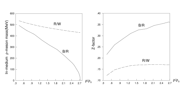
Figure 8: The in-medium $\rho$-meson mass and $Z$ factor obtained in [66] for $\Gamma_{t}=0$.

Kim et al. [66] showed that the dispersion relation (115) gives the two states, which have $\rho$-meson quantum numbers, with the spectral weight

$$Z=\left(1-\frac{\partial}{\partial q_{0}}{\rm Re}\,\Sigma_{\rho N^{*}N}\right)^{-1}$$ (118)

and that one of them can be interpreted as an in-medium vector meson whose mass decreases. Figure 8 shows the results with $\Gamma_{t}=0$. R/W indicates that $m_{\rho}$ in (117) is the free mass and B/R indicates that $q_{0}/m_{\rho}$ in (117) is replaced by 1, i.e., replacing $m_{\rho}$ by $m_{\rho}^{\star}$. Note that $q_{0}$ i.e., the in-medium $\rho$-meson mass, cannot go to zero at any density as seen in R/W of Fig. 8 if $m_{\rho}$ in the denominator of (117) is fixed. It matches neither BR scaling [14] nor the prediction that $m_{\rho}^{\star}\rightarrow 0$ at the chiral transition point [45]. Brown et al. [65] suggested the replacement of $m_{\rho}$ in (117) by $m_{\rho}^{\star}$ in order to go from Rapp et al.’s hadronic theory to BR scaling which predicts zero vector meson mass at some high density. B/R of Fig. 8 shows that in-medium $\rho$-meson mass goes to zero near $\rho\sim 2.75\rho_{0}$ as predicted in [45]. The study of the schematic model [65, 66] provides how BR scaling can be interpolated from a hadronic rescattering description.

5 Effective Lagrangian with BR scaling

If the large anomalous dimension of the scalar field in FTS1 is a symptom of a strong-coupling regime, it suggests that one should redefine the vacuum in such a way that the fluctuations around the new vacuum become weak-coupling. This is the basis of the BR scaling introduced in [14]. The basic idea is to fluctuate around the “vacuum” defined at $\rho\approx\rho_{0}$ characterized by the quark condensate $\langle\bar{q}q\rangle_{\rho}\equiv\langle\bar{q}q\rangle^{\star}$. This theory was developed with a chiral Lagrangian implemented with the trace anomaly of QCD as seen in the last section. The Lagrangian used was the one valid in the large $N_{c}$-limit of QCD and hence given entirely in terms of boson fields from which baryons arise as solitons (skyrmions): Baryon properties are therefore dictated by the structure of the bosonic Lagrangian, thereby leading to a sort of universal scaling between mesons and baryons. One can see, using a dilated chiral quark model, that BR scaling is a generic feature also at high temperature in the large $N_{c}$ limit [69].

In this description, one is approximating the complicated strong interaction process at a given nuclear matter density in terms of “quasiparticle” excitations for both baryons and bosons in medium. This means that the properties of fermions and bosons in medium at $\rho\approx\rho_{0}$ are given in terms of tree diagrams with the properties defined in terms of the masses and coupling constants universally determined by the quark condensates at that density.

The question then is: How can one marry the FTS1 Lagrangian with the BR-scaled Lagrangian? The next question is how to identify BR-scaled parameters with the Landau parameters. In this section we will provide some answers to these two questions.

5.1 A Hybrid BR-scaled model

As a first attempt to answer these questions, we consider the hybrid model in which the ground state is given by the mean field of the FTS1 Lagrangian ${{\mathcal{L}}}_{FTS1}$ and the fluctuation around the ground state is described by the tree diagrams of the BR-scaled Lagrangian $\Delta{{\mathcal{L}}}$,

$${{\mathcal{L}}}^{eff}={{\mathcal{L}}}_{FTS1}+\Delta{{\mathcal{L}}}.$$ (119)

This model with the canonical parameters (T1) for the ground state and a BR-scaled fluctuation Lagrangian in the non-strange flavor sector was recently used by Li, Brown, Lee, and Ko [26] for describing simultaneously nucleon flow and dilepton production in heavy ion collisions. The nucleon flow is sensitive to the parameters of the baryon sector, in particular, the repulsive nucleon vector potential at high density whereas the dilepton production probes the parameters of the meson sector. With a suitable momentum dependence implemented to the FTS1 mean field equation of state, the nucleon flow comes out in good agreement with experiments. Furthermore the scaling of the nucleon mass in the FTS1 theory in dense medium, say, at $\rho\sim 3\rho_{0}$, is found to be essentially the same as that given by the NJL model. Therefore we can conclude that the nucleon in FTS1 scales in the same way as BR scaling.

The dilepton production involves both baryon and meson properties, the former in the scaling of the nucleon mass and the latter in the scaling of the vector meson ($\rho$) mass. The equation of state correctly describing the nucleon flow and the BR-scaled vector meson mass is found to fit the dilepton data equally well, comparable to the fit obtained in [17] using Walecka mean field. What is important in this process is the scalar mean field which governs the BR scaling and hence the production rate comes out essentially the same for FTS1 and Walecka mean fields. The delicate interplay between the attraction and the repulsion that figures importantly in the compression modulus does not play an important role in the dilepton process.

Let us see how the particles behave in the background of the FTS1 ground state given by ${{\mathcal{L}}}_{FTS1}$. The nucleon of course scales à la BR as mentioned above. We can say nothing on the pion and the $\rho$ meson with the FTS1 theory. However there is nothing which would preclude the $\rho$ scaling à la BR and the pion non-scaling within the scheme. What is encoded in the FTS1 theory is the behavior of the $\omega$ and the scalar $S$ which figure importantly in Walecka mean fields. Let us therefore focus on these two fields in medium near normal nuclear matter density.

We have already shown in subsection 3.5.3 that the mass of the scalar field $S$ drops less rapidly than BR scaling for $d>2$. One can think of this as a screening of the four-Fermi interaction in the scalar channel that arises when the scalar meson with the BR-scaled mass is integrated out. This feature and the property of the $\omega$ field can be seen by the toy model of the FTS1 Lagrangian (that includes terms corresponding up to three-body forces)

$${\mathcal{L}}_{toyFTS1}={\mathcal{L}}_{BR}+\frac{m_{\omega}^{2}}{2}(2+\eta)\frac{\phi}{S_{0}}\omega^{2}-\frac{m_{s}^{2}\phi^{3}}{3S_{0}}$$ (120)

where

$${\mathcal{L}}_{BR} = \bar{N}(i\gamma_{\mu}(\partial^{\mu}+ig_{v}\omega^{\mu})-M+g_{s}\phi)N$$ (121)

$$+\frac{m_{\omega}^{2}}{2}\omega^{2}(1-\frac{2\phi}{S_{0}})-\frac{m_{s}^{2}}{2}\phi^{2}(1-\frac{2\phi}{3S_{0}}).$$

We have written ${{\mathcal{L}}_{BR}}$ such that the BR scaling is incorporated at mean field level as

$$\Phi(\rho)=\frac{M^{\star}}{M}=\frac{m_{s}^{\star}}{m_{s}}=\frac{m_{\omega}^{\star}}{m_{\omega}}\approx 1-\frac{\phi}{S_{0}}$$ (122)

with

$$S_{0}=\langle 0|S|0\rangle=M/g_{s}.$$ (123)

Here we are ignoring the deviation of the scaling of the effective nucleon mass (denoted later as $m_{N}^{\star}$) from the universal scaling $\Phi(\rho)$ [21]. This will be incorporated in the next subsection. We can see from (120) that the FTS1 theory brings in an additional repulsive three-body force coming from a cubic scalar field term while if one takes $\eta=-2$, the $\omega$ field will have a BR scaling mass in nuclear matter. Fit to experiments favors $\eta\approx-1/2$ instead of $-2$, thus indicating that the FTS1 theory requires a many-body suppression of the repulsion due to the $\omega$ exchange two-body force. (In the simple model with BR scaling that we will construct below, we shall use this feature by introducing a “running” vector coupling $g_{v}^{\star}$ that drops as a function of density.) The effective $\omega$ mass may be written as

$$m_{\omega}^{\star 2}\approx[1+\eta\frac{\phi_{0}}{S_{0}}]m_{\omega}^{2}.$$ (124)

For $\eta<0$, we have a falling $\omega$ mass corresponding to BR scaling (modulo, of course, the numerical value of $\eta$). In FTS1, there is a quartic term $\sim\omega^{4}$ which is attractive and hence increases the $\omega$ mass. In fact, because of the attractive quartic $\omega$ term, we have

$$\frac{m_{\omega}^{\star}}{m_{\omega}}\approx 1.12$$ (125)

at the saturation density with T1 parameter set. This would seem to suggest that due to higher polynomial (many-body) effects, the $\omega$ mass does not follow BR scaling in medium. Furthermore the $\omega$ effective mass increases slowly around this equilibrium value. On the other hand Klingl, Waas, and Weise’s recent sum rule analysis on current correlation function [71, 72] follows BR scaling. It shows that effective $\omega$ meson mass scales down by about 15$\%$ at normal nuclear matter density from its free value. We will discuss the shift of vector meson mass in medium in detail in Section 5.6.

5.2 Model with BR scaling

The above hybrid model suggests how to construct an effective Lagrangian model that implements BR scaling and contains the same physics as the FTS1 theory. The crucial point is that such a Lagrangian is to give in the mean field the chiral liquid soliton solution. This can be done by making the following replacements in (121):

$$M-g_{s}\phi_{0} \rightarrow M^{\star},$$

$$m_{\omega}^{2}(1-\frac{2\phi_{0}}{S_{0}}) \rightarrow {m_{\omega}^{\star}}^{2},$$

$$m_{s}^{2}(1-\frac{2\phi_{0}}{S_{0}}) \rightarrow {m_{s}^{\star}}^{2}$$ (126)

and write

$${\mathcal{L}}_{BR} = \bar{N}(i\gamma_{\mu}(\partial^{\mu}+ig_{v}\omega^{\mu})-M^{\star}+h\phi)N$$ (127)

$$-\frac{1}{4}F_{\mu\nu}^{2}+\frac{1}{2}(\partial_{\mu}\phi)^{2}+\frac{{m^{\star}_{\omega}}^{2}}{2}\omega^{2}-\frac{{m^{\star}_{s}}^{2}}{2}\phi^{2}$$

with

$$\frac{M^{\star}}{M}=\frac{m_{\omega}^{\star}}{m_{\omega}}=\frac{m_{s}^{\star}}{m_{s}}=\Phi(\rho).$$ (128)

The additional term $\bar{N}h\phi N$ is put in to account for the difference between the Landau mass $m_{L}^{\star}$ to be given later and the BR scaling mass $M^{\star}$. In the chiral Lagrangian approach with BR scaling, the difference comes through the Fock term involving non-local pion exchange. This will be discussed further in the next chapter. For simplicity we will take the scaling in the form

$$\Phi(\rho)=\frac{1}{1+y\rho/\rho_{0}}$$ (129)

with $y=0.28$ so as to give $\Phi(\rho_{0})=0.78$ (corresponding to $k_{F}=260$ MeV) found in QCD sum rule calculations [73], as well as from the in-medium GMOR relation [47].

Note that the Lagrangian (127) treated at the mean field level would give a Walecka-type model with the meson masses replaced by the BR scaling mass.
Now in order to describe nuclear matter in the spirit of the FTS1 theory, we introduce terms cubic and higher in $\omega$ and $\phi$ fields to be treated as perturbations around the BR background as

$${\mathcal{L}}_{n-body}=a\phi\omega^{2}+b\phi^{3}+c\omega^{4}+d\phi^{4}+e\phi^{2}\omega^{2}+\cdots$$ (130)

where $a$ – $e$ are “natural” (possibly density-dependent) constants to be determined. By inserting for the $\phi$ and $\omega$ fields the solutions of the static mean field equations given by ${{{\mathcal{L}}}_{BR}}$,

$${m_{s}^{\star}}^{2}\bar{\phi} = h\sum_{i}\bar{N}_{i}N_{i}$$ (131)

$${m^{\star}_{\omega}}^{2}\bar{\omega}_{0} = g_{v}\sum_{i}N_{i}^{\dagger}N_{i}$$ (132)

we see that at the mean-field level, ${{\mathcal{L}}_{n-body}}$ generates three- and higher-body forces with the exchanged masses density-dependent à la BR. Note that at this point, the scaling factor $\Phi$ and the mean field value (131) are not necessarily locked to each other by self-consistency.

As the first trial, we will consider the drastically simplified model by dropping the n-body term (130) and minimally modifying the BR Lagrangian (127). We shall do this by letting as mentioned above the vector coupling “run” as a function of density. For this, we use the observation made in [26] that the nucleon flow probing higher density requires that $g_{v}^{\star}/m_{\omega}^{\star}$ be independent of density at low densities and decrease slightly at high densities. We shall therefore take, to simulate this particular many-body correlation effect, the vector coupling to scale as

$$\frac{g_{v}^{\star}}{g_{v}}=\frac{1}{1+z\rho/\rho_{0}}$$ (133)

with $z$ equal to or slightly greater than $y$. The $h$ is assumed not to scale although it is easy to take into account the density dependence if necessary.

The scaling (133) seems at odds with the prediction made with the Skyrme model [74] where using the Skyrme model with the quartic Skyrme term inversely proportional to the coupling $e^{2}$, it was found that

$$\frac{e}{e^{\star}}\sim\sqrt{\frac{g_{A}^{\star}}{g_{A}}}.$$

It is tempting to identify (via $SU(6)$ symmetry) $e$ with $g_{v}$ that we are discussing here since the Skyrme quartic term can formally be obtained from a hidden gauge-symmetric Lagrangian by integrating out the $\rho$ meson field. If this were correct, one would predict that the vector coupling increases – and not decreases – as density increases since we know that $g_{A}^{\star}$ is quenched in dense matter. This identification could be too naive and incomplete in two respects, however. First of all, this skyrmion formula is a large-$N_{c}$ relation and secondly the Skyrme quartic term embodies all short-distance physics in one dimension-four term in a derivative expansion. Thus the constant $1/e$ must represent a lot more than just the vector-meson ($\rho$) degree of freedom. Furthermore we are concerned with the $\omega$ degree of freedom which in a naive derivative expansion would give a six-derivative term. The BR-scaled model we are constructing should involve not only short-distance physics presumably represented by the $1/e$ term (consistent with the understanding that the quenching of $g_{A}$ is a short-distance phenomena) but also longer-range correlations. Therefore the qualitative difference should surprise no one.

The truncated Lagrangian that we shall consider then is

$${\mathcal{L}}_{BR} = \bar{N}(i\gamma_{\mu}(\partial^{\mu}+ig_{v}^{\star}\omega^{\mu})-M^{\star}+h\phi)N$$ (134)

$$-\frac{1}{4}F_{\mu\nu}^{2}+\frac{1}{2}(\partial_{\mu}\phi)^{2}+\frac{{m^{\star}_{\omega}}^{2}}{2}\omega^{2}-\frac{{m^{\star}_{s}}^{2}}{2}\phi^{2}.$$

As suggested in [75, 42, 5], chiral in-medium Lagrangians can be brought to a form equivalent to a Walecka-type model. The scalar field appearing here transforms as a singlet, not as the fourth component of $O(4)$ of the linear sigma model. As it stands, the Lagrangian (134) does not look chirally invariant. This is because we have dropped pion fields which play no role in the ground state of nuclear matter. In considering fluctuations around the ground state, they (and other pseudo-Goldstone fields such as kaons) should be reinstated. The chiral singlet $\omega$ field and $\phi$ field can be considered as auxiliary fields brought in from a Lagrangian consisting of multi-Fermion field operators [5] via a Hubbard-Stratonovich transformation.

Since we treat density-dependent parameters, we must be careful in thermodynamic consistency. After showing the way to treat density-dependent parameters in the next section, we display the results of our model for nuclear matter properties. We will argue in the next subsection that the energy density from (5.3) is independent of the way how the parameters move as density increases.

5.3 Thermodynamic consistency in medium

In this subsection we address the issue of thermodynamic consistency of the Lagrangian (134) treated in the mean field approximation. For instance, it is not obvious that the presence of the density-dependent parameters in the Lagrangian does not spoil the self-consistency of the model, in particular, energy-momentum conservation in the medium and also certain relations of Fermi-liquid structure of the matter. The purpose of this section is to show that there is no inconsistency in doing a field theory with BR scaling masses and other parameters. This point has not been fully appreciated by workers in the field. The Euler-Lagrange equations of motion are in the same as the ones that arise from the field for the Lagrangian wherein the masses and constants are not BR scaling. While this procedure gives correct energy density, pressure and compression modulus, the energy-momentum conservation is not automatically assured. In fact, if one were to compute the pressure from the energy-density ${{\mathcal{E}}}$, one would find that it does not give $\frac{1}{3}<T_{ii}>$ (where $T_{\mu\nu}$ is the conserved energy-momentum tensor and the bra-ket means the quantity evaluated in the mean-field approximation as defined before) unless one drops certain terms without justification. This suggests that it is incorrect to take the masses and coupling constants independent of fields in deriving, by Noether theorem, the energy-momentum tensor. So the question is: how do we treat the field dependence of the BR scaling masses and constants?

One possible solution to this problem is as follows. In Section 4.2, the density dependence of the Lagrangian arose as the vacuum expectation value of the scalar field $\chi$ that figures in the QCD trace anomaly. By vacuum we mean the state of baryon number zero modified from that of true vacuum by the strong influence of the baryons in the system. See later for more on this point. It corresponded to the condensate of a quarkonium component of the scalar $\chi$ with the gluonium component – which lies higher than the chiral scale – integrated out. It was assumed to scale in dense medium in a Skyrmion-type Lagrangian subject to chiral symmetry. Now in the language of a chiral Lagrangian consisting of the nucleonic matter field $N$ with other massive fields integrated out, this scalar condensate would be some function of the vacuum expectation value of $\bar{N}N$ or $\bar{N}\gamma_{0}N$ coming from multi-Fermion field operators mentioned above. How these four-Fermi and higher-Fermi field terms can lead to BR scaling in the framework of chiral perturbation theory was discussed in [5]. We shall follow this strategy in this paper leaving other possibilities (such as dependence on the mean fields of the massive mesons) for later investigation. For this, it is convenient to define

$$\check{\rho}u^{\mu}\equiv\bar{N}\gamma^{\mu}N$$ (135)

with unit fluid 4-velocity

$$u^{\mu}=\frac{1}{\sqrt{1-\mbox{\boldmath$v$}^{2}}}(1,\mbox{\boldmath$v$})=\frac{1}{\sqrt{\rho^{2}-\mbox{\boldmath$j$}^{2}}}(\rho,\mbox{\boldmath$j$})$$ (136)

with the baryon current density

$$\mbox{\boldmath$j$}=<\bar{N}\mbox{\boldmath$\gamma$}N>$$ (137)

and the baryon number density

$$\rho=<N^{\dagger}N>=\sum_{i}n_{i}.$$ (138)

We will take $n_{i}$ to be given by the Fermi distribution function, $n_{i}=\theta(k_{F}-|\mbox{\boldmath$k$}_{i}|)$ at $T=0$. We should replace $\rho$ in (134) by $\check{\rho}$ for consistency of the model. The definition of $\check{\rho}$ makes our Lagrangian Lorentz-invariant which will later turn out to be useful in deriving relativistic Landau formulas. With this, the Euler-Lagrange equation of motion for the nucleon field is

$$\frac{\delta{\mathcal{L}}}{\delta\bar{N}} = \frac{\partial{\mathcal{L}}}{\partial\bar{N}}+\frac{\partial{\mathcal{L}}}{\partial\check{\rho}}\frac{\partial\check{\rho}}{\partial\bar{N}}$$ (139)

$$= [i\gamma^{\mu}(\partial_{\mu}+ig_{v}^{\star}\omega_{\mu}-iu_{\mu}\check{\Sigma})-M^{\star}+h\phi]N$$

$$= 0$$

with

$$\check{\Sigma} = \frac{\partial{\mathcal{L}}}{\partial\check{\rho}}$$

$$= m_{\omega}^{\star}\omega^{2}\frac{\partial m_{\omega}^{\star}}{\partial\check{\rho}}-m_{s}^{\star}\phi^{2}\frac{\partial m_{s}^{\star}}{\partial\check{\rho}}-\bar{N}\omega^{\mu}\gamma_{\mu}N\frac{\partial g_{v}^{\star}}{\partial\check{\rho}}-\bar{N}N\frac{\partial M^{\star}}{\partial\check{\rho}}.$$

This additional term which may be related to what is referred to in many-body theory as “rearrangement terms” plays a crucial role in what follows. The equations of motion for the bosonic fields are

$$(\partial^{\mu}\partial_{\mu}+m_{s}^{\star 2})\phi = h\bar{N}N$$ (141)

$$\partial_{\nu}F_{\omega}^{\nu\mu}+m_{\omega}^{\star 2}\omega^{\mu} = g_{v}^{\star}\bar{N}\gamma^{\mu}N.$$ (142)

We start with the conserved canonical energy-momentum tensor constructed a la Noether from the Lagrangian (134):

$$T^{\mu\nu} = i\bar{N}\gamma^{\mu}\partial^{\nu}N+\partial^{\mu}\phi\partial^{\nu}\phi-\partial^{\mu}\omega_{\lambda}\partial^{\nu}\omega^{\lambda}$$ (143)

$$-\frac{1}{2}[(\partial\phi)^{2}-m_{s}^{\star 2}\phi^{2}-(\partial\omega)^{2}+m_{\omega}^{\star 2}\omega^{2}-2\check{\Sigma}\bar{N}{\hbox to0.0pt{$u$\hss}\thinspace/}N]g^{\mu\nu}.$$

We shall compute thermodynamic quantities from (143) using the mean field approximation which amounts to taking

$$N = \frac{1}{\sqrt{V}}\sum_{i}a_{i}\sqrt{\frac{E_{\kappa_{i}}+m_{N}^{\star}}{2E_{\kappa_{i}}}}\left(\begin{array}[]{c}\chi\\ \frac{\mbox{\boldmath$\sigma$}\cdot\mbox{\boldmath$\kappa$}_{i}}{E_{\kappa_{i}}+m_{N}^{\star}}\chi\end{array}\right)\exp{(i\mbox{\boldmath$\kappa$}_{i}\cdot\mbox{\boldmath$x$}-i(g_{v}^{\star}\omega_{0}-u_{0}\Sigma+E_{i})t)}$$ (146)

$$h\phi = C_{h}^{2}<\bar{N}N>=C_{h}^{2}\sum_{i}n_{i}\frac{m_{N}^{\star}}{\sqrt{\mbox{\boldmath$\kappa$}^{2}_{i}+m_{N}^{\star 2}}}$$ (147)

$$g_{v}^{\star}\omega = C_{v}^{2}(\rho,\mbox{\boldmath$j$})=C_{v}^{2}\sum_{i}n_{i}\left(1,\frac{\mbox{\boldmath$\kappa$}_{i}}{\sqrt{\mbox{\boldmath$\kappa$}^{2}_{i}+m_{N}^{\star 2}}}\right)$$

where $a_{i}$ is the annihilation operator of the nucleon $i$, with

$$n_{i}=<a^{\dagger}_{i}a_{i}>,$$ (148)

and

$$\Sigma = \langle\check{\Sigma}\rangle,$$ (149)

$$\mbox{\boldmath$\kappa$}_{i} \equiv \mbox{\boldmath$k$}_{i}-C_{v}^{2}\mbox{\boldmath$j$}+\mbox{\boldmath$u$}\Sigma,$$ (150)

and

$$E_{\kappa_{i}} = \sqrt{\mbox{\boldmath$\kappa$}^{2}_{i}+m_{N}^{\star 2}}.$$ (151)

$\chi$ is the spinor and $\sigma$ is the Pauli matrix. We have defined

$$C_{v}(\check{\rho})\equiv\frac{g_{v}^{\star}(\check{\rho})}{m_{\omega}^{\star}(\check{\rho})}$$ (152)

and

$$C_{h}(\check{\rho})\equiv\frac{h}{m_{s}^{\star}(\check{\rho})}\equiv\frac{1}{\tilde{C}_{h}(\check{\rho})}.$$ (153)

In this approximation, the energy density is

$${\mathcal{E}} = <T^{00}>$$

$$= <i\bar{N}\gamma^{0}\partial^{0}N+\frac{1}{2}m_{s}^{\star 2}\phi^{2}-\frac{1}{2}m_{\omega}^{\star 2}\omega^{2}+\check{\Sigma}\bar{N}{\hbox to0.0pt{$u$\hss}\thinspace/}N>$$

$$= \frac{1}{2}C_{v}^{2}(\rho^{2}+\mbox{\boldmath$j$}^{2})+\frac{1}{2}\tilde{C}_{h}^{2}(m_{N}^{\star}-M^{\star})^{2}+\sum_{l}n_{l}\sqrt{\mbox{\boldmath$\kappa$}^{2}_{l}+m_{N}^{\star 2}}-\Sigma\mbox{\boldmath$u$}\cdot\mbox{\boldmath$j$}.$$

Note that the $\Sigma$-dependent terms cancel out in the comoving frame ($\mbox{\boldmath$v$}=0$), so that the resulting energy-density is identical to what one would obtain from the Lagrangian in the mean field with the density-dependent parameters taken as field-independent quantities.
Given the energy density (5.3), the pressure can be calculated by (at $T=0$)

$$p = -\frac{\partial E}{\partial V}=\rho^{2}\frac{\partial{\mathcal{E}}/\rho}{\partial\rho}=\mu\rho-{\mathcal{E}}$$ (155)

$$= \frac{1}{2}C_{v}^{2}(\rho)\rho^{2}-\Sigma_{0}\rho-\frac{1}{2}\tilde{C}_{h}^{2}(\rho)(m_{N}^{\star}-M^{\star}(\rho))^{2}$$

$$-\frac{\gamma}{2\pi^{2}}\left(E_{F}(\frac{m_{N}^{\star 2}}{8}k_{F}-\frac{1}{12}k_{F}^{3})-\frac{m_{N}^{\star 4}}{8}{\rm ln}[(k_{F}+E_{F})/m_{N}^{\star}]\right)$$

where $\mu$ is the chemical potential – the first derivative of the energy density with respect to $\rho$ in the comoving frame ($\mbox{\boldmath$v$}=0$):

$$\mu\equiv\frac{\partial}{\partial\rho}{\mathcal{E}}|_{\mbox{\boldmath$v$}=0}=C_{v}^{2}\rho+E_{F}-\Sigma_{0}$$ (156)

with $E_{F}=\sqrt{k_{F}^{2}+m_{N}^{\star 2}}$ and $\Sigma_{0}=\langle\check{\Sigma}\rangle_{\mbox{\boldmath$v$}=0}$. To check that this is consistent, we calculate the pressure from the energy-momentum tensor (143) in the mean field at $T=0$:

$$p_{t} \equiv \frac{1}{3}<T_{ii}>_{\mbox{\boldmath$v$}=0}$$

$$= \frac{1}{3}\langle i\bar{N}\gamma_{i}\partial_{i}N-\frac{1}{2}(m_{\omega}^{\star 2}\omega^{2}-m_{s}^{\star 2}\phi^{2}-2\check{\Sigma}N^{\dagger}N)g_{ii}\rangle_{\mbox{\boldmath$v$}=0}$$

$$= \frac{1}{2}C_{v}^{2}(\rho)\rho^{2}-\frac{1}{2}\tilde{C}_{h}^{2}(\rho)(m_{N}^{\star}-M^{\star}(\rho))^{2}-\Sigma_{0}\rho$$

$$-\frac{\gamma}{2\pi^{2}}\left(E_{F}(\frac{m_{N}^{\star 2}}{8}k_{F}-\frac{1}{12}k_{F}^{3})-\frac{m_{N}^{\star 4}}{8}{\rm ln}[(k_{F}+E_{F})/m_{N}^{\star}]\right).$$

This agrees with (155). Thus our equation of state conserves energy and momentum.

We showed that a simple effective chiral Lagrangian with BR scaling parameters is thermodynamically consistent, a point which is important for studying nuclear matter under extreme conditions. It is clear however that this does not require that the masses appearing in the Lagrangian scale according to BR scaling only. What is shown in this subsection is that masses and coupling constants could depend on density without getting into inconsistency with general constraints of chiral Lagrangian field theory. This point is important for applying (134) to the density regime $\rho\sim 3\rho_{0}$ appropriate for the CERES dilepton experiments and also kaon production at GSI(Gesellschaft für Schwerionenforschung) where deviation from the simple BR scaling of [14] might occur.

5.4 Results

Based on the thermodynamic consistency of density-dependent effective theories proven at the mean field level, we check whether the model Lagrangian (134) can describe the infinite nuclear matter properties successfully. The characteristic properties we try to reproduce are compression modulus, $m^{\star}_{N}$, and binding energy at normal nuclear matter density, and the saturation density itself.

Table 2: Parameters for the Lagrangian (134) with $y=0.28$, $m_{s}=700{\mbox{MeV}}$, $m_{\omega}=783{\mbox{MeV}}$, $M=939{\mbox{MeV}}$

SET	$h$	$g_{v}$	$z$
S1	6.62	15.8	0.28
S2	5.62	15.3	0.30
S3	5.30	15.2	0.31

Table 3: Nuclear matter properties predicted with the parameters of Table 2. The effective nucleon mass (later identified with the Landau mass) is $m_{N}^{\star}=M^{\star}-h\phi_{0}$.

SET	$E/A-M$(MeV)	$k_{eq}$(MeV)	K(MeV)	$m_{N}^{\star}/M$	$\Phi(k_{eq})$
S1	-16.0	257.3	296	0.619	0.79
S2	-16.2	256.9	263	0.666	0.79
S3	-16.1	258.2	259	0.675	0.78

In Table 2, three sets of parameters are listed. We take the measured free-space masses for the $\omega$ and the nucleon and for the scalar $\phi$ for which the free-space mass cannot be precisely given, we take $m_{s}=700$ MeV (consistent with what is argued in [47]) so that at nuclear matter density, it comes close to what enters in the FTS1. The resulting fits to the properties of nuclear matter are given in Table 3 for the parameters given in Table 2. These results are encouraging. Considering the simplicity of the model, the model – in particular with the S2 and S3 set – is remarkably close in nuclear matter to the full FTS1. The compression modulus comes down toward the low value that is currently favored. In fact, the somewhat higher value obtained here can be easily brought down to about 200 MeV without modifying other quantities if one admits a small admixture of the residual many-body terms (130), as we shall shortly show. The effective nucleon Landau mass $m_{N}^{\star}/M\approx 0.67$ is in good agreement with what was obtained in QCD sum rule calculations [78] and also in the next section (i.e., 0.69) by mapping BR scaling to Landau-Migdal Fermi-liquid theory. We shall see below that this has strong support from low-energy nuclear properties. What is also noteworthy is that the ratio ${{\mathcal{R}}}\equiv(g_{v}^{\star}/m_{\omega}^{\star})^{2}$ forced upon us – though not predicted – is independent of the density (set S1) or slightly decreasing with density (sets S2 and S3), as required in the nucleon flow data as found by Li, Brown, Lee and Ko [26]. In FTS1 theory, it is the higher polynomial terms in $\omega$ and $\phi$ defining the mean fields that are responsible for the reduction in ${{{\mathcal{R}}}}$ needed in [26]. In Dirac-Brueckner-Hartree-Fock theory, it is found [79] that while ${{{\mathcal{R}}}}$ takes the free-space value ${{{\mathcal{R}}}}_{0}$ for $\rho\approx\rho_{0}$, it decreases to ${{{\mathcal{R}}}}\approx 0.64{{{\mathcal{R}}}}_{0}$ at $\rho\approx 3\rho_{0}$ due to rescattering terms which in our language would correspond to the many-body correlations.

The assumption that the many-body correlation terms in (130) can be entirely subsumed in the dropping vector coupling may seem too drastic. Let us see what small residual three-body and four-body terms in (130) as many-body correlations (over and above what is included in the running vector coupling constant) can do to nuclear matter properties. For convenience we rewrite (130) by inserting dimensional factors as

$${\mathcal{L}}_{n-body} = \frac{\eta_{0}}{2}m^{2}_{\omega}\frac{\phi}{f_{\pi}}\omega^{2}-\frac{\kappa_{3}}{3!}m_{s}^{2}\frac{\phi^{3}}{f_{\pi}}$$

$$+\frac{\zeta_{0}}{4!}g_{v}^{2}\omega^{4}-\frac{\kappa_{4}}{4!}m_{s}^{2}\frac{\phi^{4}}{f_{\pi}^{2}}+\frac{\eta_{1}}{2}m^{2}_{\omega}\frac{\phi^{2}}{f_{\pi}^{2}}\omega^{2}$$

and demand that the coefficients $\eta$, $\zeta$ and $\kappa$ so defined be natural. The results of this analysis are given in Table 4 and Fig. 9 for various values of the residual many-body terms and compared with those of the truncated model (134) with S3 parameter set. The coefficients are chosen somewhat arbitrarily to bring our points home, with no attempt made for a systematic fit. (It would be easy to fine-tune the parameters to make the model as close as one wishes to FTS1 theory.) It should be noted that while the equilibrium density or Fermi momentum $k_{eq}$, the effective nucleon mass $m_{N}^{\star}$ and the binding energy $B$ stay more or less unchanged, within the range of the parameters chosen, from what is given by the BR-scaled model (134) with the S3 parameters, the compression modulus $K$ can be substantially decreased by the residual many-body terms. Figure 9 shows that as expected, lowering of the compression modulus is accompanied by softening of the equation of state at $\rho>\rho_{0}$. While the equilibrium property other than the compression modulus is insensitive to the many-body correlation terms, the equation of state at larger density can be quite sensitive to them. This is because for the generic parameters chosen, the $m_{N}^{\star}$ can vanish at a given density above $\rho_{0}$ at which the approximation is expected to break down and hence the resulting value cannot be trusted. The B2 and B4 models do show this instability at $\rho\mathrel{\raise 1.29167pt\hbox{$>$\kern-7.5pt\lower 4.30554pt\hbox{$\sim$}}}1.5\rho_{0}$. (See Fig. A.1.)

Table 4: Effect of many-body correlations on nuclear matter properties using the Lagrangian (134) $+$ (5.4). We have fixed the free-space masses $m_{s}=700{\mbox{MeV}},m_{\omega}=783{\mbox{MeV}},M=939{\mbox{MeV}}$ and set $\eta_{1}=0$ for simplicity. The equilibrium density $k_{eq}$, the compression modulus $K$, and the binding energy $B=M-E/A$ are all given in units of MeV.

SET	$h$	$g_{v}$	$y$	$z$	$\eta_{0}$	$\zeta_{0}$	$\kappa_{3}$	$\kappa_{4}$	$k_{eq}$	$\frac{m_{N}^{*}}{M}$	$K$	$B$
S3	5.30	15.2	0.28	0.31					258.2	0.675	259	16.1
B1	5.7	15.3	0.28	0.30			0.5	-4.9	256.0	0.666	209	16.2
B2	5.7	15.3	0.28	0.30	-0.055	0.18			257.3	0.661	201	16.1
B3	5.6	15.27	0.28	0.30			0.31	-4.1	259.1	0.659	185	16.1
B4	5.6	15.3	0.28	0.31			0.9	-8.1	256.4	0.669	191	16.1
C1	5.7	15.3	0.28	0.30	-0.05	0.155			256.3	0.665	218	16.2
C2	5.8	15.3	0.28	0.30	-0.11	0.35			256.1	0.662	161	16.2

Figure 9: $E/A-M$ vs. $\rho$ for FTS1 theory (“T1” parameter), the “S3”, “B1” and “B3” models defined in Table 4.

It is quite encouraging that the simple minimal model (134) with BR scaling captures so much of the physics of nuclear matter. Of course, by itself, there is no big deal in what is obtained by the truncated model: It is not a prediction. What is not trivial, however, is that once we have a Lagrangian of the form (134) which defines the mean fields, then we are able to control with some confidence the background around which we can calculate fluctuations, which was the principal objective we set at the beginning of this approach. The power of the simple Lagrangian is that we can now treat fluctuations at higher densities as one encounters in heavy-ion collisions, not just at an equilibrium point. The description of such fluctuations does not suffer from the sensitivity with which the equation of state depends at $\rho>\rho_{0}$ on the many-body correlation terms (130).

The simple Lagrangian (134) embodies the effective field theory of QCD discussed by Furnstahl, Serot, and Tang [11] anchored on general considerations of chiral symmetry. This Lagrangian should be viewed as an effective Lagrangian that results from two successive renormalization group “decimations”, one leading to a chiral liquid structure [39] at the chiral symmetry scale and the other with respect to the Fermi surface [8, 9]. The advantage of (134) is that it can, on the one hand, be connected to Landau Fermi-liquid fixed point theory of nuclear matter and, on the other hand, be extrapolated to the regime of hadronic matter produced under extreme conditions as encountered in relativistic heavy ion processes. It would, for instance, allow one, starting from the ground state of nuclear matter, to treat on the same footing the dilepton processes observed in CERES experiments as explained in [17] and kaon production at SIS(Schwerionen-Synchrotron) energy and kaon condensation in dense matter relevant to the formation of compact stars as discussed in [80].

5.5 Landau Fermi-liquid properties of the BR-scaled model

The next issue we address is the connection between the mean-field theory of the chiral Lagrangian (5.2) and Landau’s Fermi-liquid fixed point theory as formulated in Section 3.3. As far as we know, this connection is the only means available to implement chiral symmetry of QCD in dense matter based on effective field theory. For this, we shall follow closely Matsui’s analysis of Walecka model in mean field [81] exploiting the similarity of our model to the latter.

5.5.1 Quasiparticle interactions

The quasiparticle energy $\varepsilon_{i}$ and quasiparticle interaction $f_{ij}$ are, respectively, given by first and second derivatives with respect to $n_{i}$:

$$\varepsilon_{i} = \frac{\partial{\mathcal{E}}}{\partial n_{i}},$$ (159)

$$f_{ij} = \frac{\partial\varepsilon_{i}}{\partial n_{j}}.$$ (160)

A straightforward calculation gives

$$\varepsilon_{i} = C_{v}^{2}\rho+\sqrt{\mbox{\boldmath$\kappa$}_{i}^{2}+m_{N}^{\star 2}}+C_{v}\rho^{2}\frac{\partial C_{v}}{\partial n_{i}}-C_{v}^{2}\mbox{\boldmath$j$}^{2}\frac{\partial C_{v}}{\partial n_{i}}$$ (161)

$$+\tilde{C}_{h}(m_{N}^{\star}-M^{\star})^{2}\frac{\partial\tilde{C}_{h}}{\partial n_{i}}-\tilde{C}_{h}^{2}(m_{N}^{\star}-M^{\star})\frac{\partial M^{\star}}{\partial n_{i}}-\Sigma\mbox{\boldmath$u$}\cdot\frac{\partial\mbox{\boldmath$j$}}{\partial n_{i}}$$

and

$$f_{ij} = \frac{\partial\varepsilon_{i}}{\partial n_{j}}|_{\mbox{\boldmath$j$}=\mbox{\boldmath$v$}=0}$$ (162)

$$= C_{v}^{2}+4C_{v}\rho\frac{\partial C_{v}}{\partial\rho}+\frac{m_{N}^{\star}}{E_{i}}\frac{\partial m_{N}^{\star}}{\partial n_{j}}+\rho^{2}[(\frac{\partial C_{v}}{\partial\rho})^{2}+C_{v}\frac{\partial^{2}C_{v}}{\partial\rho^{2}}]$$

$$+(m_{N}^{\star}-M^{\star})^{2}[(\frac{\partial\tilde{C}_{h}}{\partial\rho})^{2}+\tilde{C}_{h}\frac{\partial^{2}\tilde{C}_{h}}{\partial\rho^{2}}]+2\tilde{C}_{h}\frac{\partial\tilde{C}_{h}}{\partial\rho}(m_{N}^{\star}-M^{\star})\frac{\partial}{\partial n_{j}}(m_{N}^{\star}-M^{\star})$$

$$-2\tilde{C}_{h}\frac{\partial\tilde{C}_{h}}{\partial\rho}(m_{N}^{\star}-M^{\star})\frac{\partial M^{\star}}{\partial\rho}-\tilde{C}_{h}^{2}\frac{\partial M^{\star}}{\partial\rho}\frac{\partial}{\partial n_{j}}(m_{N}^{\star}-M^{\star})-\tilde{C}_{h}^{2}(m_{N}^{\star}-M^{\star})\frac{\partial^{2}M^{\star}}{\partial\rho^{2}}$$

$$-(C_{v}^{2}-\frac{\Sigma_{0}}{\rho})\frac{\mbox{\boldmath$k$}_{i}}{E_{i}}\cdot\frac{\partial\mbox{\boldmath$j$}}{\partial n_{j}}$$

with $E_{i}=\sqrt{\mbox{\boldmath$k$}_{i}^{2}+m_{N}^{\star 2}}$. Note that $C_{v}$, $\tilde{C}_{h}$, and $M^{\star}$ are functions of

$$\langle\check{\rho}\rangle=u_{0}\rho-\mbox{\boldmath$u$}\cdot\mbox{\boldmath$j$}$$ (163)

in the mean field approximation. In arriving at (162), we have used the observation that in the limit $\mbox{\boldmath$j$}\rightarrow 0$, we have

$$\frac{\partial u_{0}}{\partial n_{i}} \rightarrow 0,$$

$$\frac{\partial^{2}u_{0}}{\partial n_{i}\partial n_{j}} \rightarrow \frac{1}{\rho^{2}}\frac{\partial\mbox{\boldmath$j$}}{\partial n_{i}}\cdot\frac{\partial\mbox{\boldmath$j$}}{\partial n_{j}},$$

$$\frac{\partial\mbox{\boldmath$u$}}{\partial n_{i}} \rightarrow \frac{1}{\rho}\frac{\partial\mbox{\boldmath$j$}}{\partial n_{i}},$$

$$\frac{\partial\langle\check{\rho}\rangle}{\partial n_{i}} \rightarrow 1,$$

$$\frac{\partial^{2}\langle\check{\rho}\rangle}{\partial n_{i}\partial n_{j}} \rightarrow -\frac{1}{\rho}\frac{\partial\mbox{\boldmath$j$}}{\partial n_{i}}\cdot\frac{\partial\mbox{\boldmath$j$}}{\partial n_{j}}$$

and that if $f$ is taken to be a function of the expectation value of $\check{\rho}$, then as $\mbox{\boldmath$j$}\rightarrow 0$, we have

$$\frac{\partial f}{\partial n_{i}} = \frac{\partial f}{\partial\langle\check{\rho}\rangle}\frac{\partial\langle\check{\rho}\rangle}{\partial n_{i}}$$ (164)

$$\rightarrow \frac{\partial f}{\partial\rho}$$

$$\frac{\partial^{2}f}{\partial n_{i}\partial n_{j}} = \frac{\partial^{2}f}{\partial\langle\check{\rho}\rangle^{2}}\frac{\partial\langle\check{\rho}\rangle}{\partial n_{i}}\cdot\frac{\partial\langle\check{\rho}\rangle}{\partial n_{j}}+\frac{\partial f}{\partial\langle\check{\rho}\rangle}\frac{\partial^{2}\langle\check{\rho}\rangle}{\partial n_{i}\partial n_{j}}$$ (165)

$$\rightarrow \frac{\partial^{2}f}{\partial\rho^{2}}-\frac{1}{\rho}\frac{\partial f}{\partial\rho}\frac{\partial\mbox{\boldmath$j$}}{\partial n_{i}}\cdot\frac{\partial\mbox{\boldmath$j$}}{\partial n_{j}}.$$

In the absence of the baryon current, $\mbox{\boldmath$j$}=0$, the quantities $\frac{\partial m_{N}^{\star}}{\partial n_{j}}$ and $\frac{\partial\mbox{\boldmath$j$}}{\partial n_{j}}$ simplify to

$$\frac{\partial m_{N}^{*}}{\partial n_{j}}=\frac{\frac{\partial M^{\star}}{\partial\rho}-2C_{h}\frac{\partial C_{h}}{\partial\rho}\sum_{l}n_{l}\frac{m_{N}^{\star}}{E_{l}}-C_{h}^{2}\frac{m_{N}^{\star}}{E_{j}}}{1+C_{h}^{2}\sum_{l}n_{l}\frac{\mbox{\boldmath$k$}_{l}^{2}}{E_{l}^{3/2}}}$$ (166)

and

$$\frac{\partial\mbox{\boldmath$j$}}{\partial n_{j}}=\frac{\frac{\mbox{\boldmath$k$}_{j}}{E_{j}}}{1+(C_{v}^{2}-\frac{\Sigma_{0}}{\rho})\sum_{l}n_{l}\frac{\frac{2}{3}\mbox{\boldmath$k$}_{l}^{2}+m_{N}^{\star 2}}{E_{l}^{3/2}}}.$$ (167)

Writing in the standard way

$$f_{l}=(2l+1)\int\frac{d\Omega}{4\pi}P_{l}(\frac{\mbox{\boldmath$k$}_{i}\cdot\mbox{\boldmath$k$}_{j}}{k_{F}^{2}})f_{ij}(|\mbox{\boldmath$k$}_{i}|=|\mbox{\boldmath$k$}_{j}|=k_{F}),$$ (168)

we see that the last term in (162) contributes to $f_{1}$ and the sum of the rest at the Fermi surface (i.e. $|\mbox{\boldmath$k$}_{j}|=k_{F}$) to $f_{0}$. So

$$F_{0} \equiv \frac{\lambda k_{F}E_{F}}{2\pi^{2}}f_{0}=\frac{3E_{F}}{k_{F}}\rho f_{0}$$

$$= \frac{3E_{F}}{k_{F}}\rho\big{[}C_{v}^{2}+4C_{v}\rho\frac{\partial C_{v}}{\partial\rho}+\frac{m_{N}^{\star}}{E_{F}}\frac{\partial m_{N}^{\star}}{\partial n_{j}}+\rho^{2}\{(\frac{\partial C_{v}}{\partial\rho})^{2}+C_{v}\frac{\partial^{2}C_{v}}{\partial\rho^{2}}\}$$

$$+(m_{N}^{\star}-M^{\star})^{2}\left\{(\frac{\partial\tilde{C}_{h}}{\partial\rho})^{2}+\tilde{C}_{h}\frac{\partial^{2}\tilde{C}_{h}}{\partial\rho^{2}}\right\}+2\tilde{C}_{h}\frac{\partial\tilde{C}_{h}}{\partial\rho}(m_{N}^{\star}-M^{\star})\frac{\partial}{\partial n_{j}}(m_{N}^{\star}-M^{\star})$$

$$-2\tilde{C}_{h}\frac{\partial\tilde{C}_{h}}{\partial\rho}(m_{N}^{\star}-M^{\star})\frac{\partial M^{\star}}{\partial\rho}-\tilde{C}_{h}^{2}\frac{\partial M^{\star}}{\partial\rho}\frac{\partial}{\partial n_{j}}(m_{N}^{\star}-M^{\star})-\tilde{C}_{h}^{2}(m_{N}^{\star}-M^{\star})\frac{\partial^{2}M^{\star}}{\partial\rho^{2}}\big{]}$$

and

$$F_{1} \equiv \frac{\lambda k_{F}E_{F}}{2\pi^{2}}f_{1}$$ (170)

$$= -\frac{3(C_{v}^{2}-\frac{\Sigma_{0}}{\rho})\rho}{E_{F}+(C_{v}^{2}-\frac{\Sigma_{0}}{\rho})\rho}.$$

5.5.2 Some relations for relativistic Fermi-liquid

Here we bridge the model (134) to relativistic Fermi-liquid theory. For it we will show that the thermodynamic properties of any model like (134), which has density-dependent parameters and is Walecka-type, can be described in terms of relativistic Landau parameters derived from the mean field approximation of the model in the same way as in Section 2.3.

First let us calculate the compression modulus K defined by

$$K\equiv 9\rho\frac{\partial^{2}{\mathcal{E}}(\mbox{\boldmath$j$}=0)}{\partial\rho^{2}}.$$ (171)

It comes out to be

$$K = \frac{3k_{F}^{2}}{E_{F}}+9\rho[C_{v}^{2}+4C_{v}\rho\frac{\partial C_{v}}{\partial\rho}+\frac{m_{N}^{\star}}{E_{F}}\frac{\partial m_{N}^{\star}}{\partial\rho}+\rho^{2}\{(\frac{\partial C_{v}}{\partial\rho})^{2}+C_{v}\frac{\partial^{2}C_{v}}{\partial\rho^{2}}\}$$

$$+(m_{N}^{\star}-M^{\star})^{2}\{(\frac{\partial\tilde{C}_{h}}{\partial\rho})^{2}+\tilde{C}_{h}\frac{\partial^{2}\tilde{C}_{h}}{\partial\rho^{2}}\}+2\tilde{C}_{h}\frac{\partial\tilde{C}_{h}}{\partial\rho}(m_{N}^{\star}-M^{\star})\frac{\partial}{\partial\rho}(m_{N}^{\star}-M^{\star})$$

$$-2\tilde{C}_{h}\frac{\partial\tilde{C}_{h}}{\partial\rho}(m_{N}^{\star}-M^{\star})\frac{\partial M^{\star}}{\partial\rho}-\tilde{C}_{h}^{2}\frac{\partial M^{\star}}{\partial\rho}\frac{\partial}{\partial\rho}(m_{N}^{\star}-M^{\star})-\tilde{C}_{h}^{2}(m_{N}^{\star}-M^{\star})\frac{\partial^{2}M^{\star}}{\partial\rho^{2}}]$$

Comparing (5.5.1) and (5.5.2), we obtain Eq. (29);

$$K=\frac{3k_{F}^{2}}{E_{F}}(1+F_{0}).$$ (173)

In our model

$$k_{F}\left(\frac{\partial k_{i}}{\partial\varepsilon_{i}}\right)_{k=k_{F},\mbox{\boldmath$v$}=0}=E_{F}\equiv\sqrt{k_{F}^{2}+m_{N}^{\star 2}}.$$ (174)

It is verified that our model satisfies the relativistic Landau Fermi-liquid formula for the compression modulus (29).

As shown in Section 2.3, the relativistic Landau liquid satisfies the mass relation (40);

$$k_{F}\left(\frac{\partial k_{i}}{\partial\varepsilon_{i}}\right)_{k=k_{F},\vec{v}=0}=\mu(1+F_{1}/3).$$

One can see from Eqs. (156), (170), and (174) that (40) is satisfied exactly in our model.

And lastly the relativistic relation for the first sound velocity (2.3.3) is satisfied automatically since (29) and (40) are satisfied in our model. So all the relativistic Landau Fermi-liquid relations in Section 2.3 are satisfied with density-dependent Walecka-type models like (134).

5.5.3 Discussions

The crucial question is really how to understand the scaling masses and constants as one varies temperature and density as considered in [14]. If one takes the basic assumption that the chiral Lagrangian in the mean field with BR scaling parameters corresponds to Landau’s Fermi-liquid fixed point theory, then one should consider first fixing the Fermi momentum $k_{F}$ and let renormalization group flow come to the fixed points of the effective mass $m_{L}^{\star}$ for the nucleon and Landau parameters ${\mathcal{F}}$ [8]. In this case, the scaling quantities would seem to be dependent upon $\Lambda/k_{F}$, not on the fields entering into the effective Lagrangian. This paper however shows that if one wants to approach the Fermi-liquid fixed point theory starting from an effective chiral Lagrangian of QCD, it is necessary to take into account the fact that the scaling arises from the effect of multi-Fermi interactions figuring in chiral Lagrangians as implied by chiral perturbation theory described in [5]. This is probably due to the fact that we are dealing with two-stage “decimations” in the present problem – with the Fermi surface formed from a chiral Lagrangian as a nontopological soliton (i.e., “chiral liquid” [39]) – in contrast to condensed matter situations where one starts ab initio with the Fermi surface without worrying about how the Fermi surface is formed. Our result suggests that there will be a duality in describing processes manifesting the scaling behavior. In other words, the change of “vacuum” by density exploited in [14] could equally be represented by a certain (possibly infinite) set of interactions among hadrons – e.g., four-Fermi and higher-Fermi terms in chiral Lagrangians – canonically taken into account in many-body theories starting from the usual matter-free vacuum. A notable evidence may be found in the two plausible explanations of the low mass enhancement in CERES dilepton yields in terms of scaling vector meson masses [17] and in terms of hadronic interactions giving rise to increased widths [63, 82]. Recently the relation between two descriptions are discussed by Brown et al. [65] and also by Kim et al. [66]. It is argued that the description based on the reaction dynamics and on the meson spectral function should be reliable at low density where the effective degrees of freedom are hadrons and have no contradiction with the description on BR scaling. There should however be a “crossover” region at higher density at which BR scaling will become more efficient or we should go over to constituent quarks. How to relate the two description in the “crossover” density regime remains an open problem.

In discussing the properties of dense matter, such as the BR scaling of masses and coupling constants, e.g., $f_{\pi}^{\star}$ , we have been using a Lagrangian which preserves Lorentz invariance. This seems to be at odds with the fact that the medium breaks Lorentz symmetry. One would expect for instance that the space and time components of a current would be characterized by different constants. Specifically such quantities as $g_{A}$, $f_{\pi}$ etc. would be different if they were associated with the space component or time component of the axial current. So a possible question is: How is the medium-induced symmetry breaking accommodated in the formalism which will be discussed in the next section?

Section 5.3 and this section provide the answer to this question. Here the argument is given in an exact parallel to Walecka mean field theory of nuclear matter. One writes an effective Lagrangian with all symmetries of QCD which in the mean field defines the parameters relevant to the state of matter with density. The parameters that become constants (masses, coupling constants etc.) at given density are actually functionals of chiral invariant bilinears in the nucleon fields. When the scalar field $\phi$ and the bilinear ${\psi}^{\dagger}\psi$, where $\psi$ is the nucleon field, develop a non-vanishing expectation value Lorentz invariance is broken and the time and space components of a nuclear current pick up different constants. This is how for instance the Gamow-Teller constant $g_{A}$ measured in the space component of the axial current is quenched in medium while the axial charge measured in the axial charge transitions is enhanced as described in the next chapter. If one were to calculate the pion decay constant in medium, one would also find that the quantity measured in the space component is different from the time component. The way Lorentz-invariant Lagrangians figure in nuclear physics is in some sense similar to what happens in condensed matter physics.

5.6 Mesons in medium

It should be recalled that we extracted the scaling parameter $\Phi$ from the in-medium property of the vector mesons. Here we will present evidences for the predicted scaling in the meson masses. There are some preliminary experimental indications for decrease in matter of the $\rho$ meson mass in recent nuclear experiments [83, 84] but we expect more definitive results from future experiments at GSI and other laboratories. In fact, this is currently a hot issue in connection with the recent dilepton data coming from relativistic heavy ion experiments at CERN(European Organization for Nuclear Research).

When heavy mesons such as the vector mesons $\rho$, $\omega$ and the scalar $\sigma$ are reinstated in the chiral Lagrangian, then the mass parameters of those particles in the Lagrangian, when written in a chirally invariant way, are supposed to appear with star and are assumed to scale according to Eq. (112). The question is: What is the physical role of these mass parameters? If we assume that the mesons behave also like quasiparticles, that is, like weakly interacting particles with the “dropping masses,” then physical observables will be principally dictated by the tree diagrams of those particles endowed with the scaling masses. In this case, the masses figuring in the Lagrangian could be identified in some sense as “effective” masses of the particles in the matter. This line of reasoning was used in the work of Li, Ko and Brown [17] to interpret the low mass enhancement of the CERES data [15]. As discussed in Section 5.2, this treatment is consistent with an effective Lagrangian which in the mean field approximation yields the nuclear matter ground state as well as fluctuations around the ground state. The parameters of the theory, as well as their density dependence are determined by the properties of the ground state. The work of this section shows that this scheme is internally consistent. However we emphasize that the scaling we have established is for the mesons that are highly off-shell and it may not be applied to mesons that are near on-shell without further corrections (e.g., widths etc.).

Suppose one probes the propagation of an $\omega$ meson in nuclear medium as in HADES(High Acceptance Di-Electron Spectrometer) or TJNAF(Thomas Jefferson National Accelerator Facility) experiments, say through dilepton production. The $\omega$’s will decay primarily outside of the nuclear medium, but let us suppose that experimental conditions are chosen so that the leptons from the $\omega$ decaying inside dense matter can be detected. See [85] for discussions on this issue. The question is whether the dileptons will probe the BR-scaled mass or the quantity given by (125). The behavior of the $\omega$ mass would differ drastically in the two scenarios. A straightforward application of FTS1 theory would suggest that at a density $\rho\mathrel{\raise 1.29167pt\hbox{$<$\kern-7.5pt\lower 4.30554pt\hbox{$\sim$}}}\rho_{0}$, the $\omega$ mass as “seen” by the dileptons will increase slightly instead of decrease. Since in FTS1 theory, the vector coupling $g_{v}$ does not scale, this means that $(g_{v}^{\star}/m_{\omega}^{\star})$ will effectively decrease. On the other hand if the vector coupling constant drops together with the mass at increasing density as in the BR scaling model, the situation could be quite different, particularly if dileptons are produced at a density $\rho\sim 3\rho_{0}$ as in the CERES experiments: The $\omega$ will then be expected to BR-scale up to the phase transition. It has been recently suggested [86] that at some high density, Lorentz symmetry can be spontaneously broken giving rise to light $\omega$ mesons as “almost Goldstone” bosons when a small explicit Lorentz symmetry breaking term via chemical potential is introduced. By introducing the term, they assume a state which is chirally symmetric ($\langle\bar{q}q\rangle=0$) but breaks Lorentz symmetry ($\langle q^{\dagger}q\rangle\neq 0$). The assumed state is metastable at $\mu<\mu_{c}$ but becomes a global minimum at $\mu>\mu_{c}$. At $\mu>\mu_{c}$, $\omega$ would become light but not massless due to the explicit breaking. Such mesons could be a source of copious dileptons at some density higher than normal matter density. Thus measuring the $\omega$ mass shift could be a key test of the BR scaling idea as opposed to the FTS1-type interpretations. This interesting issue will be studied in forthcoming experiments at GSI and TJNAF. It is interesting that the dropping $\omega$ mass is also found in a recent QCD sum rule calculation based on current correlation functions by Klingl, Kaiser and Weise [71] who, however, do not see the dropping of the $\rho$ mass because of the large broadening of $\rho$ peak. If we can describe the $\omega$ meson in medium as a quasiparticle an $\omega$-nuclear bound state is feasible even in light nuclei [72]. The process like ⁷Li(d,³He)${}^{6}_{\omega}$He is expected to be seen in GSI [87] if such a bound state exists.

6 Fermi-liquid theory vs. chiral Lagrangian

6.1 Electromagnetic current

We will here give a brief derivation of the Landau-Migdal formula for the convection current for a particle of momentum $k$ sitting on top of the Fermi sea responding to a slowly varying electromagnetic (EM) field. We will then analyze it in terms of the specific degrees of freedom that contribute to the current. This will be followed by a description in terms of a chiral Lagrangian as discussed in [21]. This procedure will provide the link between the two approaches.

6.1.1 Landau-Migdal formula for the convection current

Following Landau’s original reasoning adapted by Migdal to nuclear systems, we start with the convection current given by

$$\mbox{\boldmath$J$}=\sum_{\sigma,\tau}\int\frac{d^{3}p}{(2\pi)^{3}}(\mbox{\boldmath$\nabla$}_{p}\varepsilon_{p})n_{p}\frac{1}{2}(1+\tau_{3})$$ (175)

where the sum goes over the spin $\sigma$ and isospin $\tau$ which in spin- and isospin-saturated systems may be written as a trace over the $\sigma$ and $\tau$ operators. More precisely, this is a matrix element of the current operator corresponding to the response to the EM field of a nucleon (proton or neutron) sitting on top of the Fermi sea. The sum over spin and isospin and the momentum integral go over all occupied states up to the valence particle. What we want is a current operator and it is deduced after the calculation is completed. One can of course work directly with the operator but the result is the same. We consider a variation of the distribution function from that of an equilibrium state

$$n_{p}=n_{p}^{0}+\delta n_{p},$$ (176)

where the superscript $0$ refers to equilibrium. The variation of the distribution function induces a variation of the quasiparticle energy

$$\varepsilon_{p}=\varepsilon_{p}^{0}+\delta\varepsilon_{p}.$$ (177)

In the equilibrium state the current is zero by symmetry, so we have

$$J = \sum_{\sigma,\tau}\int\frac{d^{3}p}{(2\pi)^{3}}\left((\mbox{\boldmath$\nabla$}_{p}\varepsilon^{0}_{p})\delta n_{p}+(\mbox{\boldmath$\nabla$}_{p}\delta\varepsilon_{p})n^{0}_{p}\right)\frac{1}{2}(1+\tau_{3}),$$ (178)

$$= \sum_{\sigma,\tau}\int\frac{d^{3}p}{(2\pi)^{3}}\left((\mbox{\boldmath$\nabla$}_{p}\varepsilon^{0}_{p})\delta n_{p}-(\mbox{\boldmath$\nabla$}_{p}n^{0}_{p})\delta\varepsilon_{p})\right)\frac{1}{2}(1+\tau_{3})$$

to linear order in the variation. We consider a nucleon added at the Fermi surface of a system in its ground state. Then

$$\delta n_{p}=\frac{1}{V}\delta^{3}(\mbox{\boldmath$p$}-\mbox{\boldmath$k$\/})\frac{1\pm\tau_{3}}{2}$$ (179)

and

$$\mbox{\boldmath$\nabla$}_{p}n^{0}_{p}=-\frac{\mbox{\boldmath$p$}}{k_{F}}\delta(p-k_{F})$$ (180)

where $k$ with $|\mbox{\boldmath$k$\/}|=k_{F}$ is the momentum of the quasiparticle. The modification of the quasiparticle energies due to the additional particle is given by

$$\delta\varepsilon_{p}=\sum_{\sigma^{\prime},\tau^{\prime}}\int\frac{d^{3}p^{\prime}}{(2\pi)^{3}}f_{p,p^{\prime}}\delta n_{p^{\prime}\sigma^{\prime}\tau^{\prime}}.$$ (181)

Combining (2), (178), (179) and (181) one finds that the first term of (178) gives the operator

$$\mbox{\boldmath$J$}^{(1)}=\frac{\mbox{\boldmath$k$\/}}{m_{L}^{\star}}\frac{1+\tau_{3}}{2},$$ (182)

where $k$ is taken to be at the Fermi surface. The second term yields

$$\delta\mbox{\boldmath$J$}=\delta\mbox{\boldmath$J$}_{s}+\delta\mbox{\boldmath$J$}_{v}=\frac{\mbox{\boldmath$k$\/}}{M}\left(\frac{\tilde{F}_{1}+\tilde{F}_{1}^{\prime}\tau_{3}}{6}\right),$$ (183)

where

$$\delta\mbox{\boldmath$J$}_{s} = \frac{\mbox{\boldmath$k$}}{m_{L}^{\star}}\frac{1}{2}\frac{F_{1}}{3},$$ (184)

$$\delta\mbox{\boldmath$J$}_{v} = \frac{\mbox{\boldmath$k$\/}}{m_{L}^{\star}}\frac{\tau_{3}}{2}\frac{F^{\prime}_{1}}{3}=\frac{\mbox{\boldmath$k$\/}}{m_{L}^{\star}}\frac{\tau_{3}}{2}\frac{F_{1}}{3}+\frac{\mbox{\boldmath$k$\/}}{m_{L}^{\star}}\frac{\tau_{3}}{2}\frac{F^{\prime}_{1}-F_{1}}{3}.$$ (185)

For convenience, let’s define

$$\tilde{F}_{l}\equiv(M/m_{L}^{\star})F_{l}$$ (186)

with analogous definitions of $\tilde{F}_{l}^{\prime}$, etc.. It gives another representation of (41)

$$\frac{M}{m_{L}^{\star}}=1-\frac{\tilde{F}_{1}}{3}.$$ (187)

Putting everything together we recover the well known result of Migdal [31, 33]

$$\mbox{\boldmath$J$}=\frac{\mbox{\boldmath$k$\/}}{M}g_{l}=\frac{\mbox{\boldmath$k$\/}}{M}\left(\frac{1+\tau_{3}}{2}+\frac{1}{6}(\tilde{F}^{\prime}_{1}-\tilde{F}_{1})\tau_{3}\right),$$ (188)

where

$$g_{l}=\frac{1+\tau_{3}}{2}+\delta g_{l}$$ (189)

is the orbital gyromagnetic ratio and

$$\delta g_{l}=\frac{1}{6}(\tilde{F}^{\prime}_{1}-\tilde{F}_{1})\tau_{3}.$$ (190)

Thus, the renormalization of $g_{l}$ is purely isovector. This is due to Galilean invariance, which implies a cancellation in the isoscalar channel.

We have derived Migdal’s result using standard Fermi-liquid theory arguments. This result can also be obtained [88] by using the Ward identity, which follows from gauge invariance of the electro-magnetic interaction. This is of course physically equivalent to the above formulation. We shall now identify specific hadronic contributions to the current (188) in two ways: the Fermi-liquid theory approach and the chiral Lagrangian approach.

6.1.2 Pionic contribution

In Fermi-liquid theory approach, all we need to do is to compute the Landau parameter $F_{1}$ from the pion exchange. The one-pion-exchange contribution to the quasiparticle interaction is

$$f^{\pi-exch.}_{\mbox{\boldmath$p$}\sigma\tau,\mbox{\boldmath$p$}^{\prime}\sigma^{\prime}\tau^{\prime}}=\frac{1}{3}\frac{f^{2}}{m_{\pi}^{2}}\frac{\mbox{\boldmath$q$}^{2}}{\mbox{\boldmath$q$}^{2}+m_{\pi}^{2}}\left(S_{12}(\mbox{\boldmath$\hat{q}$})+\frac{1}{2}(3-\mbox{\boldmath$\sigma$}\cdot\mbox{\boldmath$\sigma$}^{\prime})\right)\frac{3-\mbox{\boldmath$\tau$}\cdot\mbox{\boldmath$\tau$}^{\prime}}{2}$$ (191)

where $\mbox{\boldmath$q$}=\mbox{\boldmath$p$}-\mbox{\boldmath$p$}^{\prime}$ and $f=g_{\pi NN}(m_{\pi}/2M)\approx 1$. In a relativistic formulation sketched in Appendix B, we can Fierz the one-pion exchange. Done in this way, the Fierzed scalar channel is canceled by a part of the vector channel and the remaining vector channel makes a natural contribution to the pionic piece of $F_{1}$. The one-pion-exchange contribution to the Landau parameter relevant for the convection current is

$$\frac{F_{1}(\pi)}{3}=-F_{1}^{\prime}(\pi)=-\frac{3f^{2}m_{L}^{\star}}{8\pi^{2}k_{F}}I_{1}$$ (192)

where

$$I_{1}=\int_{-1}^{1}dx\frac{x}{1-x+\frac{m_{\pi}^{2}}{2k_{F}^{2}}}=-2+(1+\frac{m_{\pi}^{2}}{2k_{F}^{2}}){\rm ln}(1+\frac{4k_{F}^{2}}{m_{\pi}^{2}}).$$ (193)

Note that $F_{1}(\pi)$ satisfies

$$F_{1}(\pi)=-\frac{3m_{L}^{\star}}{k_{F}}\left.\frac{d\Sigma_{\pi}(p)}{dp}\right|_{p=k_{F}}$$ (194)

with one-pion-exchange Fock contribution to the self-energy $\Sigma(p)$ and includes the higher order contribution in $m_{L}^{\star}$. Thus, from Eq. (190), the one-pion-exchange contribution to the gyromagnetic ratio is

$$\delta g_{l}^{\pi}=\frac{M}{k_{F}}\frac{f^{2}}{4\pi^{2}}I_{1}\tau_{3}.$$ (195)

In the next subsubsection we include contributions also from other degrees of freedom.

Let’s obtain the convection current from a chiral Lagrangian and compare it with the results given above. In absence of other meson degrees of freedom, we can simply calculate Feynman diagrams given by a chiral Lagrangian defined in matter-free space. Nonperturbative effects due to the presence of heavy mesons introduce a subtlety that will be treated below.

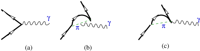
Figure 10: Feynman diagrams contributing to the EM convection current in effective chiral Lagrangian field theory. Figure (a) is the single-particle term and (b, c) the next-to-leading chiral order pion-exchange current term. Figure (c) does not contribute to the convection current; it renormalizes the spin gyromagnetic ratio.

In the leading chiral order, there is the single-particle contribution Fig. 10a which for a particle on the Fermi surface with the momentum $k$ is given by

$$\mbox{\boldmath$J$}_{1-body}=\frac{\mbox{\boldmath$k$\/}}{M}\frac{1+\tau_{3}}{2}.$$ (196)

Note that the nucleon mass appearing in (196) is the free-space mass $M$ as it appears in the Lagrangian, not the effective mass $m_{L}^{\star}$ that enters in the Fermi-liquid approach, (182). To the next-to-leading order, we have two soft-pion terms as discussed in [5, 89, 90, 6]. We should recall a well-known caveat here discussed already in [90]. If one were to blindly calculate the convection current coming from Fig. 10b, there would be a gauge non-invariant term that is present because the hole line is off-shell. Figure 10c contains also a gauge non-invariant term which is exactly the same as in Fig. 10b but with an opposite sign, so in the sum of the two graphs, the two cancel exactly so that only the gauge-invariant term survives. Of course we now know that the off-shell dependence is not physical and could be removed by field redefinition ab initio. To the convection current we need, only Fig. 10b contributes

$$\mbox{\boldmath$J$}_{2-body}=\frac{\mbox{\boldmath$k$\/}}{k_{F}}\frac{f^{2}}{4\pi^{2}}I_{1}\tau_{3}=\frac{\mbox{\boldmath$k$\/}}{M}\frac{1}{6}(\tilde{F}^{\prime}_{1}(\pi)-\tilde{F}_{1}(\pi))\tau_{3}.$$ (197)

We should emphasize that the Landau parameters $\tilde{F}_{1}$ and $\tilde{F}_{1}^{\prime}$ are entirely fixed by a chiral effective Lagrangian for any density.

The sum of (196) and (197) agrees precisely with the Fermi-liquid theory result (188) and (192). This formula first derived in [91] in connection with the Landau-Migdal parameter is of course the same as the Miyazawa formula [92] derived nearly half a century ago. Note the remarkable simplicity in the derivation starting from a chiral Lagrangian. However, we should caution that there are some non-trivial assumptions to go with the validity of the formula. As we will see shortly, we will not have this luxury of simplicity when other degrees of freedom enter.

6.1.3 Vector meson contributions and BR scaling

So far we have computed only the pion contribution to $g_{l}$. In nuclear physics, more massive degrees of freedom such as the vector mesons $\rho$ and $\omega$ of mass $700\sim 800$ MeV and the scalar meson $\sigma$ of mass $600\sim 700$ MeV play an important role. When integrated out from the chiral Lagrangian, they give rise to effective four-Fermion interactions:

$${{\mathcal{L}}}_{4}=\frac{C_{\phi}^{2}}{2}(\bar{N}N)^{2}-\frac{C_{\omega}^{2}}{2}(\bar{N}\gamma_{\mu}N)^{2}-\frac{C_{\rho}^{2}}{2}(\bar{N}\gamma_{\mu}\tau N)^{2}+\cdots$$ (198)

where the coefficients $C^{\prime}s$ can be identified with

$$C_{M}^{2}=\frac{g_{M}^{2}}{{m_{M}}^{2}}\ \ \ {\rm with}\ \ \ M=\phi,\ \rho,\ \ \omega.$$ (199)

For the moment, we make no distinction as to whether one is taking into account BR scaling or not. For the Fermi-liquid approach, this is not relevant since the parameters are not calculated. However with chiral Lagrangians, we will specify the scaling which is essential. Such interaction terms are “irrelevant” in the renormalization group flow sense but can make crucial contributions by becoming “marginal” in some particular kinematic situation. A detailed discussion of this point can be found in [8]. The effective four-Fermion interactions play a key role in stabilizing the Fermi-liquid state and leads to the fixed points for the Landau parameters. (The other fixed-point quantity, i.e. the effective mass, is put in by fiat to keep the density fixed.) In the two-nucleon systems studied in [7], they enter into the next-to-leading order term of the potential, which is crucial in providing the cut-off independence found for cut-off masses $\mathrel{\raise 1.29167pt\hbox{$>$\kern-7.5pt\lower 4.30554pt\hbox{$\sim$}}}m_{\pi}$.

Again it suffices to compute the Landau parameters coming from the velocity-dependent part of heavy meson exchanges in the Fermi-liquid theory approach. We treat the effective four-Fermion interaction (198) in the Hartree approximation. Then the only velocity-dependent contributions are due to the current couplings mediated by $\omega$ and $\rho$ exchanges. The corresponding contributions to the Landau parameters are

$$F_{1}(\omega)=-C_{\omega}^{2}\frac{2k_{F}^{3}}{\pi^{2}M}$$ (200)

and

$$F_{1}^{\prime}(\rho)=-C_{\rho}^{2}\frac{2k_{F}^{3}}{\pi^{2}M}.$$ (201)

The derivations of relativistic $F_{1}(\omega)$ and $F_{1}^{\prime}(\rho)$ are shown in Appendix C.

Now the calculation of the convection current and the nucleon effective mass with the interaction (198) in the Landau method goes through the same way as in the case of the pion. The net result is just Eq. (188) including the contribution of the contact interactions (200,201), i.e.,

$$\tilde{F}_{1} = \tilde{F}_{1}(\pi)+\tilde{F}_{1}(\omega),$$ (202)

$$\tilde{F}^{\prime}_{1} = \tilde{F}^{\prime}_{1}(\pi)+\tilde{F}^{\prime}_{1}(\rho).$$ (203)

Similarly, the nucleon effective mass is determined by (41) with

$$F_{1}=F_{1}(\pi)+F_{1}(\omega).$$ (204)

In chiral Lagrangina approach the most efficient way to bring in the vector mesons into the chiral Lagrangian is to implement BR scaling in the parameters of the Lagrangian. We shall take the masses of the relevant degrees of freedom to scale in the manner of BR as (128). Note again that $M^{\star}$ is a BR scaling nucleon mass which will turn out to be different from the Landau effective mass $m_{L}^{\star}$ [21]. For our purpose, it is more convenient to integrate out the vector and scalar fields and employ the resulting four-Fermi interactions (198). The coupling coefficients are modified compared to Eq. (199), because the meson masses are replaced by effective ones:

$$C_{M}^{2}=\frac{g_{M}^{2}}{{m_{M}^{\star}}^{2}}\ \ \ {\rm with}\ \ \ M=\phi,\ \rho,\ \ \omega.$$ (205)

The coupling constants may also scale [22] but we omit their density dependence for the moment.

The first thing we need is the relation between the BR scaling factor $\Phi$ which was proposed in [14] to reflect the quark condensate in the presence of matter and the contribution to the Landau parameter $F_{1}$ from the isoscalar vector ($\omega$) meson. For this we first calculate the Landau effective mass $m_{N}^{\star}$ in the presence of the pion and $\omega$ fields [21]

$$\frac{m_{L}^{\star}}{M}=1+\frac{1}{3}(F_{1}(\omega)+F_{1}(\pi))=\left(1-\frac{1}{3}(\tilde{F}_{1}(\omega)+\tilde{F}_{1}(\pi))\right)^{-1}.$$ (206)

Next we compute the nucleon self-energy using the chiral Lagrangian. Given the single quasiparticle energy

$$\varepsilon_{p}=\frac{p^{2}}{M^{\star}}+C_{\omega}^{2}\langle N^{\dagger}N\rangle+\Sigma_{\pi}(p),$$ (207)

we get the effective mass as in [21]

$$\frac{m_{L}^{\star}}{M}=\frac{k_{F}}{m_{N}}\left(\left.\frac{d}{dp}\varepsilon_{p}\right|_{p=k_{F}}\right)^{-1}=\left(\Phi^{-1}-\frac{1}{3}\tilde{F}_{1}(\pi)\right)^{-1}$$ (208)

from Eqs. (128), (186), and (194). Comparing (206) and (208), we obtain the important result

$$\tilde{F}_{1}(\omega)=3(1-\Phi^{-1}).$$ (209)

This is an intriguing relation. It shows that the BR factor, which was originally proposed as a precursor manifestation of the chiral phase transition characterized by the vanishing of the quark condensate at the critical point [14], is intimately related (at least up to $\rho\approx\rho_{0}$) to the Landau parameter $F_{1}$, which describes the quasiparticle interaction in a particular channel. We believe that the BR factor can be computed by QCD sum rule methods or obtained from current algebra relations such as the GMOR relation evaluated in medium. As was shown in [21], Eq. (209) implies that the BR factor governs in some, perhaps, intricate way low-energy nuclear dynamics. The equivalence discussed above between the physics of the vacuum property $\Phi$ and that of the quasiparticle interaction $F_{1}$ due to the massive vector-meson degree of freedom suggests that the “bottom-up” approach – going up in density with a Lagrangian whose parameters are fixed at zero density – and the “top-down” approach – extrapolating with a Lagrangian whose parameters are fixed at some high density – can be made equivalent at some intermediate point. If this is so in the hot and dense regime probed by relativistic heavy ion collisions, then the CERES data should also be understandable in terms of hadronic interactions without making reference to QCD variables. Because of the complexity of hadronic descriptions, it will be difficult to relate the two directly but the recent alternative explanation of the CERES data in terms of “melting of the vector mesons” inside nuclear matter manifested in the increased width of the mesons due to hadronic interactions [82] may be an indication for a possible “dual” description at low density between what is given in QCD variables (e.g., quark condensates) and what is given in hadronic variables (e.g., the Landau parameter), somewhat reminiscent of the quark-hadron duality in heavy-light-quark systems [93]. A possible mechanism that could make the link between the two descriptions was suggested recently by Brown et al. [65] and by Kim et al. [66].

In the presence of the BR scaling, a non-interacting nucleon in the chiral Lagrangian propagates with a mass $M^{\star}$, not the free-space mass $M$. Thus, the single-particle current Fig. 10a is not given by (196) but instead by

$$\mbox{\boldmath$J$}_{1-body}=\frac{\mbox{\boldmath$k$\/}}{M^{\star}}\frac{1+\tau_{3}}{2}.$$ (210)

Now the current (210) on its own does not carry conserved charge as long as $M^{\star}\neq M$. This means that two-body currents are indispensable to restore charge conservation. Note that the situation is quite different from the case of Fermi-liquid theory. In the latter case, the quasiparticle propagates with the Landau effective mass $m_{L}^{\star}$ and it is the gauge invariance that restores $m_{L}^{\star}$ to $M$. In condensed matter physics, this is related to a phenomenon that the cyclotron frequency depends on the bare mass, not on Landau effective mass. It may be referred to as Kohn effect [94]. The bare mass in Kohn effect is restored due to the quasiparticle interactions with Galilean invariance in the same way as for the convection current in Section 6.1.1 [95]. This clearly indicates that gauge invariance is more intricate when BR scaling is implemented. Indeed if the notion of BR scaling and the associated chiral Lagrangian are to make sense, we have to recover the charge conservation from higher-order terms in the chiral Lagrangian. This constitutes a strong constraint on the theory.

Let us now calculate the contributions from the pion and heavy meson degrees of freedom. The pion contributes in the same way as before, so we can carry over the previous result of Fig. 10b,

$$\vec{J}_{2-body}^{\pi}=\frac{\mbox{\boldmath$k$\/}}{M}\frac{1}{6}(\tilde{F}_{1}^{\prime}(\pi)-\tilde{F}_{1}(\pi))\tau_{3}.$$ (211)

This is of the same form as (197) obtained in the absence of BR scaling. It is in fact identical to (197) if we assume that one-pion-exchange graph does not scale in medium at least up to nuclear matter density. This assumption is supported by observations in pion-induced processes in heavy nuclei. This means that the observation that the one-pion-exchange potential does not scale implies that the constant $g_{A}^{\star}/f_{\pi}^{\star}$ remains unscaling at least up to normal nuclear matter density with non-scaling pion mass. In what follows, we will make this assumption implicitly.

The contributions from the vector meson degrees of freedom are a bit trickier. They are given by Fig. 11.

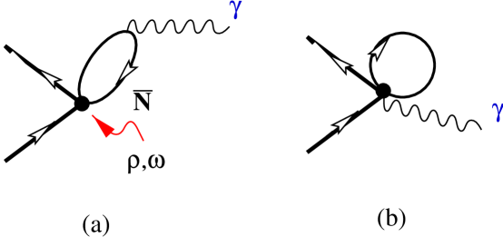
Figure 11: (a) Feynman diagram contributing to the EM convection current from four-Fermi interactions corresponding to the $\omega$ and $\rho$ channel (contact interaction indicated by the blob) in effective chiral Lagrangian field theory. Th $\bar{N}$ denotes the anti-nucleon state that is given in the chiral Lagrangian as a $1/M$ correction and the one without arrow is a Pauli-blocked or occupied state. (b) The equivalent graph in heavy-fermion formalism with the anti-nucleon line shrunk to a point.

Both the $\omega$ (isoscalar) and $\rho$ (isovector) channels contribute through the antiparticle intermediate state as shown in Fig. 11a. The antiparticle is explicitly indicated in the figure. However in the heavy-fermion formalism, the backward-going anti-nucleon line should be shrunk to a point as Fig. 11b, leaving behind an explicit $1/M$ dependence folded with a factor of nuclear density signaling the $1/M$ correction in the chiral expansion. One can interpret Fig. 11a as saturating the corresponding counter term although this has to be yet verified by writing the full set of counter terms at the same order. These terms with Fig. 11a

$$\mbox{\boldmath$J$}_{2-body}^{\omega} = \frac{\mbox{\boldmath$k$}}{M}\frac{1}{6}\tilde{F}_{1}(\omega),$$ (212)

$$\mbox{\boldmath$J$}_{2-body}^{\rho} = \frac{\mbox{\boldmath$k$}}{M}\frac{1}{6}\tilde{F}_{1}^{\prime}(\rho)\tau_{3},$$ (213)

where $\tilde{F}_{1}(\omega)$ and $\tilde{F}_{1}^{\prime}(\rho)$ are given by Eqs. (200,201) with $M$ replaced by $M^{\star}$. Their relativistic forms are given in Appendix C. The total current given by the sum of (210), (211), (212) and (213) precisely agrees with the Fermi-liquid theory result (188) when we take

$$\tilde{F}_{1} = \tilde{F}_{1}(\omega)+\tilde{F}_{1}(\pi),$$ (214)

$$\tilde{F}_{1}^{\prime} = \tilde{F}_{1}^{\prime}(\rho)+\tilde{F}_{1}^{\prime}(\pi).$$ (215)

The way in which this precise agreement comes about is nontrivial. What happens is that part of the $\omega$ channel restores the BR-scaled mass $M^{\star}$ back to the free-space mass $M$ in the isoscalar current. (It has been known since sometime that something similar happens in the standard Walecka model (without pions and BR scaling) [96]). Thus, the leading single-particle operator combines with the sub-leading four-Fermi interaction to restore the charge conservation as required by the Ward identity. This is essentially the “back-flow mechanism” which is an important ingredient in Fermi-liquid theory. We describe below the standard back-flow mechanism as given in Sec. 2.1, adapted to nuclear systems with isospin degrees of freedom, and elucidate the connection to the results obtained with the chiral Lagrangian in this subsection.

The current so constructed is valid for a process occurring very near the Fermi surface corresponding to the limit $(\omega,\mbox{\boldmath$q$})\rightarrow(0,\bf{0})$ where $q$ is the spatial momentum transfer and $\omega$ is the energy transfer. In the diagrams considered so far (Fig. 10 and 11) the order of the limiting processes does not matter. However, the particle-hole contribution, which we illustrate in Fig. 12 with the pion contribution, does depend on the order in which $q=|\mbox{\boldmath$q$}|$ and $\omega$ approach zero. Thus, in the limit $q/\omega\rightarrow 0$, the particle-hole contributions vanish whereas in the opposite case $\omega/q\rightarrow 0$, they do not.

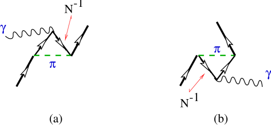
Figure 12: Particle-hole contributions to the convection current. Here backward-going nucleon line $N^{-1}$ denotes a hole. These graphs vanish in the $q/\omega\rightarrow 0$ limit.

This can be seen by examining the particle-hole propagator

$$\frac{n_{k}(1-n_{k+q})}{q_{0}+\epsilon_{k}-\epsilon_{k+q}+i\delta}-\frac{n_{k+q}(1-n_{k})}{q_{0}+\epsilon_{k}-\epsilon_{k+q}-i\delta}$$ (216)

where $(q_{0},\mbox{\boldmath$q$})$ is the four-momentum of the external (EM) field. This vanishes if we set $q\rightarrow 0$ with $q_{0}$ non-zero but its real part is non-zero if we interchange the limiting process since for $q_{0}=0$ we have

$$\frac{\mbox{\boldmath$q$}\cdot\mbox{\boldmath$\hat{k}$}}{-\mbox{\boldmath$q$}\cdot\mbox{\boldmath$k$}/M}\delta(k_{F}-k).$$ (217)

Figure 12 was computed by several authors (e.g., see [88]) and is given in the limit $\omega/q\rightarrow 0$ by

$$\mbox{\boldmath$J$}_{ph}=-\sum_{\tau^{\prime}}\langle\mbox{\boldmath$\tau$}(1)\cdot\frac{1+\tau_{3}^{\prime}}{2}\mbox{\boldmath$\tau$}(2)\rangle\int\frac{d^{3}p}{(2\pi)^{3}}\hat{\mbox{\boldmath$p$}}\delta(k_{F}-|\mbox{\boldmath$p$}|)f^{\pi}_{s}$$ (218)

where $f_{s}^{\pi}$ is the spatial and spin part of the quasiparticle interaction which is (191) and (B: Relativistic calculation of $F^{\pi}_{1}$) without isospin part $(3-\mbox{\boldmath$\tau$}\cdot\mbox{\boldmath$\tau$}^{\prime})/2$. The isospin factor is given by the Fierz transformation:

$$\sum_{\tau^{\prime}}\langle\mbox{\boldmath$\tau$}(1)\cdot\frac{1+\tau_{3}^{\prime}}{2}\mbox{\boldmath$\tau$}(2)\rangle = \sum_{\tau^{\prime}}\langle\frac{3}{4}-\frac{1}{4}\mbox{\boldmath$\tau$}\cdot\mbox{\boldmath$\tau$}^{\prime}+\frac{3}{4}{\rm tr}\,[\tau_{3}^{\prime}]-\frac{1}{4}\mbox{\boldmath$\tau$}\cdot{\rm tr}\,[\tau_{3}^{\prime}\mbox{\boldmath$\tau$}^{\prime}]\rangle$$ (219)

$$= \frac{3}{2}-\frac{1}{2}\tau_{3}.$$

Note that the factor $\frac{3}{2}$ comes from $f_{\pi}$ and $\frac{1}{2}\tau_{3}$ from $f^{\prime}_{\pi}$. In the limit that we are concerned with (i.e. $T=0$ and $\omega/q\rightarrow 0$), the particle-hole contribution to the current is

$$\mbox{\boldmath$J$}_{ph} = -\frac{1}{3\pi^{2}}\mbox{\boldmath$\hat{k}$}k_{F}^{2}(f_{1}+f_{1}^{\prime}\tau_{3})$$ (220)

$$= -\frac{\mbox{\boldmath$k$}}{M}\left(\frac{\tilde{F}_{1}(\pi)+\tilde{F}_{1}^{\prime}(\pi)\tau_{3}}{6}\right).$$

This holds in general regardless of what is being exchanged as long as the exchanged particle has the right quantum numbers. Contributions from heavy-meson exchanges are calculated in a similar way. Adding the particle-hole contribution (220) to the Fermi-liquid result (188) we obtain the current of a dressed or localized quasiparticle

$$\mbox{\boldmath$J$}_{locQP}=\frac{\mbox{\boldmath$k$}}{m_{L}^{\star}}\left(\frac{1+\tau_{3}}{2}\right).$$ (221)

Note that $\mbox{\boldmath$J$}_{ph}$ precisely cancels $\delta\mbox{\boldmath$J$}$, Eq. (183). The current $\mbox{\boldmath$J$}_{locQP}$ is the total current carried by the wave packet of a localized quasiparticle with group velocity ${\bf{v}}_{F}=\frac{\mbox{\boldmath$k$}}{m_{L}^{\star}}$. However, the physical situation corresponds to homogeneous (plane wave) quasiparticle excitations. The current carried by a localized quasiparticle equals that of a homogeneous quasiparticle excitation modified by the so called back-flow current [97]. The back-flow contribution $(\mbox{\boldmath$J$}_{locQP}-\mbox{\boldmath$J$}_{LM})$ is just the particle-hole polarization current in the $\omega/q\rightarrow 0$ limit, Eq. (220).

6.1.4 Phenomenological test

It is not obvious that the effective nucleon mass computed in the chiral Lagrangian approach is directly connected to a measurable quantity although quasielastic electron scattering from nuclei does probe some kind of effective nucleon mass and Walecka model describes such a process in terms of an effective mass. To the extent that the bulk of $m_{N}^{\star}$ is related to the condensate through BR scaling as we can see in (208), the effective mass in the chiral Lagrangian can be related to the quantity calculated in the QCD sum rule approach for in-medium hadron masses. In BR scaling, the parameter $\Phi$ is related to the scaling of the vector meson ($\rho$) mass. There are several QCD sum rule calculations for the $\rho$ meson in-medium mass starting with [98]. The most recent one which closely agrees with the GMOR formula in medium for the pion decay constant $f_{\pi}^{\star}$ (see Eq. (112)) is the one by Jin and Leinweber [73]:

$$\Phi(\rho_{0})=0.78\pm 0.08.$$ (222)

We shall take this value in what follows but one should be aware of the possibility that this value is not quite firm. A caveat to this result was recently discussed by Klingl, Kaiser, and Weise [71] who show that the QCD sum rule can be saturated without the mass shifting downward by increasing the vector meson width in medium. For a discussion of the empirical constraints on the in-medium widths of vector mesons, see Friman [99].

Given this, we can compute $m_{N}^{\star}$ using (208) for nuclear matter density since the pionic contribution $\tilde{F}_{1}(\pi)$ is known. One finds [21]

$$\frac{m_{N}^{\star}}{M}(\rho=\rho_{0})\approx 0.70.$$ (223)

This can be tested in an indirect way by looking at certain magnetic response functions of nuclei as described below. An additional evidence comes from QCD sum rule calculations. Again there are caveats in the QCD sum rule calculation for the nucleon mass even in free-space and certainly more so in medium. Nevertheless the most recent result by Furnstahl, Jin, and Leinweber [78] is rather close to the prediction (223):

$$\left(\frac{m_{N}^{\star}(\rho_{0})}{M}\right)_{QCD}=0.69^{+0.14}_{-0.07}.$$ (224)

If one writes the gyromagnetic ratio $g_{l}$ as

$$g_{l}=\frac{1+\tau_{3}}{2}+\delta g_{l}$$ (225)

then the chiral Lagrangian prediction is

$$\delta g_{l}=\frac{1}{6}(\tilde{F}_{1}^{\prime}-\tilde{F}_{1})\tau_{3}=\frac{4}{9}\left[\Phi^{-1}-1-\frac{1}{2}\tilde{F}_{1}(\pi)\right]\tau_{3}.$$ (226)

In writing the second equality we have used (192), (209) and the nonet relation $\tilde{F}^{\prime}(\rho)=\tilde{F}(\omega)/9$. At nuclear matter density, we get, using (222),

$$\delta g_{l}(\rho_{0})\approx 0.23\tau_{3}.$$ (227)

This agrees with the value extracted from the dipole sum rule in ²⁰⁹Bi [100],

$$\delta g_{l}^{proton}=0.23\pm 0.03$$ (228)

and agrees roughly with magnetic moment data in heavy nuclei. Nuclear magnetic moments are complicated due to conventional nuclear effects. To make a meaningful comparison, one would have to extract all “trivial” nuclear effects and this operation brings in inestimable uncertainties. It should be stressed that the gyromagnetic ratio provides a test for the scaling nucleon mass at $\rho\approx\rho_{0}$. It also gives a check of the relation between the baryon property on the left-hand side of Eq. (209) and the meson property on the right-hand side. Instead of using (222) as an input to calculate $\delta g_{l}$, we could take the experimental value (228) to determine, using (226), the BR scaling factor $\Phi$ at $\rho\approx\rho_{0}$. We would of course get (222), a value which is consistent with what one obtains in the QCD sum rule calculation and also in the in-medium GMOR relation.

Recall that because of the pions which provide (perturbative) non-local interactions to the Landau interaction, the Landau mass for the nucleon scales differently from that of the vector mesons. (See (112) and (208)). This difference is manifested in the skyrmion description by the fact that the coefficient of the Skyrme quartic term must also scale. In the original discussion of the scaling based on the quark condensates using the trace anomaly [14], the Skyrme quartic term was scale-invariant and hence the corresponding $g_{A}^{\star}$ was non-scaling. So the scaling implied by (208) indicates that the scaling of $g_{A}^{\star}$ is associated with the pionic degrees of freedom. This is consistent with the description based on the Landau-Migdal $g_{0}^{\prime}$ interaction between a nucleon and a $\Delta$ resonance [101, 102, 103] and also with the QCD sum rule description of Drukarev and Levin [104] who attribute about 80% of the quenching to the $\Delta-N$ effect.

If we equate the skyrmion relation [21, 74]

$$\frac{m_{N}^{\star}}{M}=\sqrt{\frac{g_{A}^{\star}}{g_{A}}}\Phi$$ (229)

to (208), we get

$$\frac{g_{A}^{\star}}{g_{A}}=\left(1+\frac{1}{3}F_{1}(\pi)\right)^{2}=\left(1-\frac{1}{3}\tilde{F}_{1}(\pi)\Phi\right)^{-2}.$$ (230)

At nuclear matter density, this predicts

$$g_{A}^{\star}(\rho_{0})\approx 1$$ (231)

and

$$\frac{g_{A}^{\star}}{g_{A}}\approx\frac{f_{\pi}^{\star}}{f_{\pi}}=\Phi.$$ (232)

We will use this relation in deriving (257). It should be emphasized that this relation, being unrelated to the vacuum property, cannot hold beyond $\rho\approx\rho_{0}$. Indeed as suggested by the scaling given in [14], $g_{A}^{\star}(\rho)\approx\alpha g_{A}$ with $\alpha$ a constant independent of density, for $\rho\mathrel{\raise 1.29167pt\hbox{$>$\kern-7.5pt\lower 4.30554pt\hbox{$\sim$}}}\rho_{0}$. It would be a good approximation to set $g_{A}^{\star}$ equal to 1 for $\rho\mathrel{\raise 1.29167pt\hbox{$>$\kern-7.5pt\lower 4.30554pt\hbox{$\sim$}}}\rho_{0}$.

Since one expects that when chiral symmetry is restored, $g_{A}$ will approach 1, it may be thought that the evidence for $g_{A}^{\star}\approx 1$ in nuclei is directly connected with chiral restoration. This is not really the case. Neither in the skyrmion picture nor in QCD sum rules is the quenching of $g_{A}$ simply related to a precursor behavior of chiral restoration. This does not however mean that the quenching of $g_{A}$ carries no information on the chiral symmetry restoration. As suggested recently by Chanfray, Delorme and Ericson [105], if one were to compute all pion-exchange-current graphs at one-loop order that contribute to the in-medium $g_{A}$, the effect of medium-induced change in the quark condesate would be largely accounted for. In a way, this argument is akin to that for the Cheshire-Cat (or dual) phenomenon we are advocating in the description of the quark condensate in terms of quasiparticles. Another issue that has generated lots of debate in the past and yet remains confusing is the interpretation of an effective constant $g_{A}^{eff}\approx 1$ actually observed in medium and heavy nuclei. The debate has been whether the observed “quenching” is due to “core polarizations” or “$\Delta$-hole effect” (or other non-standard mechanisms). Our view is that in the presence of BR scaling, both are involved. In light nuclei in which the Gamow-Teller transition takes place in low density, the tensor force is mainly operative and the core polarization (i.e., multiparticle-multihole configurations) mediated by this tensor force is expected to do most of the quenching, while the $\Delta$-hole effect directly proportional to density is largely suppressed. The typical diagrammatic representations for the second order core polarization is shown in Fig. 13.

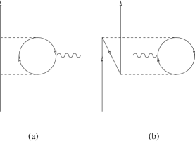
Figure 13: Examples of the second order core polarization contribution to Gamow-Teller transition. Downward nucleon line denote a hole. (a)2p1h (b)3p2h

In heavy nuclei, on the other hand, the tensor force is quenched due to BR scaling, rendering the core polarization mechanism ineffective while the increased density makes the $\Delta$-hole effect dominant. Recently Park, Jung, and Min [103] applied chiral perturbation theory to calculate $g_{A}^{\star}$ at normal nuclear matter density $\rho_{0}$.

Figure 14: The resonance-exchange graph in [103] for four-Fermi contact interaction contribution. Its Hartree contribution decreases axial vector coupling constant in medium.

Figure 15: The resonance-exchange graphs in [103] for one-pion-exchange contribution. Their Fock contributions enhance the axial vector coupling constant with incorporating the short-range correlation between nucleons.

The resonance-exchange graphs that contribute are shown in Figs. 14 and 15 and the Landau-Migdal $g_{0}^{\prime}$ effect contains both. The Hartree contribution from Fig. 14, i.e. $\Delta$-hole effect, makes $g_{A}^{\star}$ quenched and the Fock contribution from Fig. 15 enhances $g_{A}^{\star}$. The magnitude of quenching is two or three times larger than the enhancement. What is seen in nature, in our view, is the interplay between these two.

The second form of (230) shows that the quenching of $g_{A}$ in matter is quite complex, both the pionic effect and the vacuum condensate effect being confounded together. Again for the reason given above, this relation cannot be extended beyond the regime with $\rho\approx\rho_{0}$. We have no understanding of how this formula and the $\Delta$-hole mechanism of [101, 102] are related. Our effort thus far has met with no success. Understanding the connection would presumably require the short-distance physics implied by both the Landau-Migdal $g_{0}^{\prime}$ interaction and the Skyrme quartic term (which is known to be more than just what results when the $\rho$ meson is integrated out of the chiral Lagrangian).

6.2 Axial charge transition

No one has yet derived the analogue to (188) for the axial current. Attempts using axial Ward identities in analogy to the EM case have not met with success [106]. The difficulty has presumably to do with the role of the Goldstone bosons in nuclear matter which is not well understood. In this subsection, we analyze the expression for the axial charge operator obtained by a straightforward application of the Fermi-liquid theory arguments of Landau and Migdal and compare this expression with that obtained directly from the chiral Lagrangian using current algebra. For the vector current we found precise agreement between the two approaches.

6.2.1 Applying Landau quasiparticle argument

The obvious thing to do is to simply mimic the steps used for the vector current to deduce a Landau-Migdal expression for the axial charge operator. We use both methods developed above and find that they give the same result.

In free space, the axial charge operator nonrelativistically is $\sim\mbox{\boldmath$\sigma$}\cdot{\bf{v}}$ where ${\bf{v}}=\mbox{\boldmath$k$}/M$ is the velocity. In the infinite momentum frame, it is the relativistic invariant helicity ${\mbox{\boldmath$\sigma$}}\cdot\mbox{\boldmath$\hat{\nu}$}$. It is thus tempting to assume that near the Fermi surface, the axial charge operator for a local quasiparticle in a wave packet moving with the group velocity ${\bf v}_{F}=\mbox{\boldmath$k$}/m_{L}^{\star}$ is simply $\sim{\mbox{\boldmath$\sigma$}}\cdot{\bf v}_{F}$. This suggests that we take the axial charge operator for a localized quasiparticle to have the form

$${A_{0}}^{i}_{locQP}=g_{A}\frac{\mbox{\boldmath$\sigma$}\cdot\mbox{\boldmath$k$}}{m_{L}^{\star}}\frac{\tau^{i}}{2}.$$ (233)

As in the vector current case, we take (233) to be the $\omega/q\rightarrow 0$ limit of the axial charge operator. The next step is to compute the particle-hole contribution to Fig. 12 (with the vector current replaced by the axial current) in the $\omega/q\rightarrow 0$ limit. A simple calculation gives

$${A_{0}}^{i}_{ph}=-g_{A}\frac{\mbox{\boldmath$\sigma$}\cdot\mbox{\boldmath$k$}}{m_{L}^{\star}}\frac{\tau^{i}}{2}\Delta^{\prime}$$ (234)

with

$$\Delta^{\prime}=\frac{f^{2}k_{F}m_{L}^{\star}}{4m_{\pi}^{2}\pi^{2}}(I_{0}-I_{1})$$ (235)

where $I_{1}$ was defined in (193) and

$$I_{0}=\int_{-1}^{1}dx\frac{1}{1-x+\frac{m_{\pi}^{2}}{2k_{F}^{2}}}={\rm ln}\left(1+\frac{4k_{F}^{2}}{m_{\pi}^{2}}\right).$$ (236)

In an exact parallel to the procedure used for the vector current, we take the difference

$${A_{0}}^{i}_{locQP}-{A_{0}}^{i}_{ph}$$ (237)

and identify it with the corresponding “Landau axial charge”(LAC):

$${A_{0}}^{i}_{LAC}=g_{A}\frac{\mbox{\boldmath$\sigma$}\cdot\mbox{\boldmath$k$}}{m_{L}^{\star}}\frac{\tau^{i}}{2}(1+\Delta^{\prime}).$$ (238)

Let us now rederive (238) with an argument analogous to that proven to be powerful for the convection current. We shall do the calculation using the pion exchange only but the argument goes through when the contact interaction (198) is included. We begin by assuming that the axial charge – in analogy to (175) for the convection current – takes the form,

$${A_{0}}^{i}=g_{A}\sum_{\sigma\tau}\int\frac{d^{3}p}{(2\pi)^{3}}\mbox{\boldmath$\sigma$}\cdot(\mbox{\boldmath$\nabla$}_{p}\epsilon_{p})n_{p}\frac{\tau^{i}}{2}$$ (239)

where $n_{p}$ and $\epsilon_{p}$ are $2\times 2$ matrices with matrix elements

$$[n_{p}(\mbox{\boldmath$r$},t)]_{\alpha\alpha^{\prime}}=n_{p}(\mbox{\boldmath$r$},t)\delta_{\alpha\alpha^{\prime}}+\mbox{\boldmath$s$}_{p}(\mbox{\boldmath$r$},t)\cdot\mbox{\boldmath$\sigma$}_{\alpha\alpha^{\prime}},$$ (240)

and

$$[\epsilon_{p}(\mbox{\boldmath$r$},t)]_{\alpha\alpha^{\prime}}=\epsilon_{p}(\mbox{\boldmath$r$},t)\delta_{\alpha\alpha^{\prime}}+{\mbox{\boldmath$\eta$}}_{p}(\mbox{\boldmath$r$},t)\cdot\mbox{\boldmath$\sigma$}_{\alpha\alpha^{\prime}}$$ (241)

with

$${\mbox{\boldmath$s$}}_{p}(\mbox{\boldmath$r$},t)=\frac{1}{2}\sum_{\alpha\alpha^{\prime}}\mbox{\boldmath$\sigma$}_{\alpha\alpha^{\prime}}[n_{p}(\mbox{\boldmath$r$},t)]_{\alpha^{\prime}\alpha}.$$ (242)

In general $n=4$ in the spin-isospin space. But without loss of generality, we could confine ourselves to $n=2$ in the spin space with the isospin operator explicited as in Eq.(239). Then upon linearizing, we obtain from (239)

$${A_{0}}^{i}=g_{A}\sum_{\sigma\tau}\int\frac{d^{3}p}{(2\pi)^{3}}\left(\mbox{\boldmath$\sigma$}\cdot(\mbox{\boldmath$\nabla$}_{p}\epsilon^{0}_{p})\delta n_{p\sigma\tau}-\mbox{\boldmath$\sigma$}\cdot(\mbox{\boldmath$\nabla$}_{p}n^{0}_{p})\delta\epsilon_{p\sigma\tau}\right)\frac{\tau^{i}}{2}+\cdots$$ (243)

where

$$\delta n_{p\sigma\tau}=\frac{1}{V}\delta^{3}(\mbox{\boldmath$p$}-\mbox{\boldmath$k$})\frac{1+\sigma_{3}}{2}\frac{\tau^{i}}{2}$$ (244)

and

$$\delta\epsilon_{p\sigma\tau}=\sum_{\sigma^{\prime},\tau^{\prime}}\int\frac{d^{3}p^{\prime}}{(2\pi)^{3}}f_{p\sigma\tau,p^{\prime}\sigma^{\prime}\tau^{\prime}}\delta n_{p^{\prime}\sigma^{\prime}\tau^{\prime}}.$$ (245)

in analogy with (181). The equation (243) is justified if the density of polarized spins is much less than the total density of particles (assumed to hold here). The first term of (243) with (244) yields the quasiparticle charge operator

$${A_{0}}^{i}_{QP}=g_{A}\frac{\mbox{\boldmath$\sigma$}\cdot\mbox{\boldmath$k$}}{m_{L}^{\star}}\frac{\tau^{i}}{2}$$ (246)

while the second term represents the polarization of the medium, due to the pion-exchange interaction (191)

$$\delta{A_{0}}^{i}=g_{A}\frac{\mbox{\boldmath$\sigma$}\cdot\mbox{\boldmath$k$}}{m_{L}^{\star}}\frac{\tau^{i}}{2}\Delta^{\prime}.$$ (247)

The sum of (246) and (247) agrees precisely with the Landau charge (238).

It is not difficult to take into account the full Landau-Migdal interactions (2) which includes the one-pion-exchange interaction as well as other contributions to the quasiparticle interaction. Thus, the general expression is obtained by making the replacement

$$\Delta^{\prime}\rightarrow\frac{1}{3}G_{1}^{\prime}-\frac{10}{3}H_{0}^{\prime}+\frac{4}{3}H_{1}^{\prime}-\frac{2}{15}H_{2}^{\prime}$$ (248)

in (247). This combination of Fermi-liquid parameters corresponds to a $\ell=\ell^{\prime}=1,J=0$ distortion of the Fermi sea [34]. We will see later that the result obtained with the naive Landau argument may not be the whole story, since the one-pion-exchange contribution disagrees, though by a small amount, with the chiral Lagrangian prediction derived below.

6.2.2 Chiral Lagrangian prediction

We now calculate the axial charge using our chiral Lagrangian that reproduced the Landau-Migdal formula for the convection current. Consider first only the pion-exchange contribution. In this case we can take the unperturbed nucleon propagator to carry the free space mass $M$. The single-particle transition operator corresponding to Fig. 10a is given by

$${A_{0}}^{i}_{1-body}=g_{A}\frac{\mbox{\boldmath$\sigma$}\cdot\mbox{\boldmath$k$}}{M}\frac{\tau^{i}}{2}.$$ (249)

There is no contribution of the type of Fig. 10b because of the (G-)parity conservation. The only contribution to the two-body current comes from Fig. 10c and is of the form [107]

$${A_{0}}^{i}_{2-body}=g_{A}\frac{\mbox{\boldmath$\sigma$}\cdot\mbox{\boldmath$k$}}{M}\frac{\tau^{i}}{2}\Delta$$ (250)

with

$$\Delta=\frac{f^{2}k_{F}M}{2g_{A}^{2}m_{\pi}^{2}\pi^{2}}\left(I_{0}-I_{1}-\frac{m_{\pi}^{2}}{2k_{F}^{2}}I_{1}\right).$$ (251)

The factor $(1/g_{A}^{2})$ in (251) arose from replacing $\frac{1}{f_{\pi}^{2}}$ by $\frac{g_{\pi NN}^{2}}{g_{A}^{2}M^{2}}$ using the Goldberger-Treiman relation.

Now consider what happens when the vector degrees of freedom are taken into account. Within the approximation adopted, the only thing that needs be done is to implement the BR scaling. The direct intervention of the vector mesons $\rho$ and $\omega$ in the axial-charge operator is suppressed by the chiral counting, so they will be ignored here. This means that in the single-particle charge operator, all that one has to do is to replace $M$ by $M^{\star}=M\Phi$ in (249):

$${A_{0}}^{i}_{1-body}=g_{A}\frac{\mbox{\boldmath$\sigma$}\cdot\mbox{\boldmath$k$}}{M\Phi}\frac{\tau^{i}}{2}$$ (252)

and that in the two-body charge operator (250), $f_{\pi}$ should be replaced by $f_{\pi}\Phi$ and $M$ by $M\Phi$:

$${A_{0}}^{i}_{2-body}=g_{A}\frac{\mbox{\boldmath$\sigma$}\cdot\mbox{\boldmath$k$}}{M\Phi}\frac{\tau^{i}}{2}\Delta.$$ (253)

In the two-body operator, there is a factor $(g_{A}/f_{\pi})$ coming from the $\pi NN$ vertex which as mentioned before, is assumed to be non-scaling at least up to nuclear matter density [108], in consistency with the observation that the pion-exchange current does not scale in medium.

The total predicted by the chiral Lagrangian (modulo higher-order corrections) is then

$$g_{A}\frac{\mbox{\boldmath$\sigma$}\cdot\mbox{\boldmath$k$}}{M\Phi}\frac{\tau^{i}}{2}(1+\Delta).$$ (254)

which differs from the charge operator obtained by the Landau method, (238).

6.2.3 Comparison between vector and axial current

An immediate question (to which we have no convincing answer) is whether or not the difference between the two approaches – the Fermi-liquid vs. the chiral Lagrangian – is genuine or a defect in either or both of the approaches. One possible cause of the difference could be that both the assumed localized quasiparticle charge, Eq.(233), and the effective axial charge, Eq.(239), are incomplete. We have looked for possible additional terms that could contribute but we have been unable to find them. So while not ruling out this possibility, we turn to the possibility that the difference is genuine.

It is a well-known fact that the conservation of the vector current assures that the EM charge or the weak vector charge is $g_{V}=1$ but the conservation of the axial vector charge does not constrain the value of the axial charge $g_{A}$ , that is, $g_{A}$ can be anything. This is because the axial symmetry is spontaneously broken. In the Wigner phase in which the axial symmetry would be restored, one would expect that $g_{A}=1$. It therefore seems that the Goldstone structure of the “vacuum” of the nuclear matter is at the origin of the difference.

To see whether there can be basic differences, let us look at the effect of the pion field. The cancellation between the two-body current $\mbox{\boldmath$J$}_{2-body}^{\pi}$ (211) and $\mbox{\boldmath$J$}_{ph}^{\pi}$ (220) leaving only a term that changes $M^{\star}$ to $m_{L}^{\star}$ in the one-body operator with a BR scaling mass, Eq.(210), in the EM case can be understood as follows. Both terms involve the two-body interaction mediated by a pion-exchange. It is obvious how this is so in the latter. To see it in the former, we note that it involves the insertion of an EM current in the propagator of the pion. Thus the sum of the two terms corresponds to the insertion of an EM current in all internal hadronic lines of the one-pion exchange self-energy graph of the nucleon. The two-body pionic current – that together with the single-particle current preserves gauge invariance – is in turn related to the one-pion-exchange potential $V_{\pi}$. Therefore what is calculated is essentially an effect of a nuclear force. Now the point is that the density-dependent part of the sum (that is, the ones containing one hole line) – apart from a term that changes $M^{\star}$ to $m_{L}^{\star}$ in (210) – vanishes in the $\omega/q\rightarrow 0$ limit. In contrast, the cancellation between (247) and (234) in the case of the axial charge, has no corresponding interpretation. While the one-pion-exchange interaction is involved in the particle-hole term (234), (247) cannot be interpreted as an insertion of the axial vector current into the pion propagator since such an insertion is forbidden by parity. In other words, Eq.(247) does not have a corresponding Feynman graph which can be linked to a potential. We interpret this as indicating that there is no corresponding Landau formula for the axial charge in the same sense as in the vector current case.

In a chiral Lagrangian formalism, each term is associated with a Feynman diagram. As mentioned, there is no contribution to the convection current from a diagram of the type Fig. 10c (apart from a gauge non-invariant off-shell term which cancels the counter part in Fig. 10b). Instead this diagram renormalizes the spin gyromagnetic ratio. In contrast, the corresponding diagram for the axial current does contribute to the axial charge (250). As first shown in [89], the contribution from Fig.10c for both the vector current and the axial-vector current is current algebra in origin and constrained by chiral symmetry. Furthermore it does not have a simple connection to nuclear force. While the convection current is completely constrained by gauge invariance of the EM field, and hence chiral invariance has little to say, both the EM spin current and the axial charge are principally dictated by the chiral symmetry. This again suggests that the Landau approach to the axial charge cannot give the complete answer even at the level of quasiparticle description. There is however a caveat here: in the Landau approach, the nonlocal pionic and local four-Fermion interactions (198) enter together in an intricate way as we saw in the EM case. Perhaps this is also the case in the axial charge, with an added subtlety due to the presence of Goldstone pions. It is possible that the difference is due to the contribution of the four-Fermion interaction term to (248) which cancels out in the limit $\omega/q\rightarrow 0$ but contributes in the $q/\omega\rightarrow 0$ limit. This term cannot be given a simple interpretation in terms of chiral Lagrangians. Amusingly the difference between the results (see below) turns out to be small.

6.2.4 Numerical comparison

To compare the two results, we rewrite the sum of (246) and (247), i.e., “Landau axial charge” (LAC), using (41) and (192)

$${A_{0}}^{i}_{LAC}=g_{A}\frac{\mbox{\boldmath$\sigma$}\cdot\mbox{\boldmath$k$}}{M\Phi}\frac{\tau^{i}}{2}(1+\tilde{\Delta})$$ (255)

where

$$\tilde{\Delta}=\frac{f^{2}k_{F}M\Phi}{4\pi^{2}m_{\pi}^{2}}\left(I_{0}-I_{1}+\frac{3m_{\pi}^{2}}{2k_{F}^{2}}I_{1}\Phi^{-1}\right)$$ (256)

and the sum of (252) and (253), i.e., the “current-algebra axial charge”(CAAC), as

$${A_{0}}^{i}_{CAAC}=g_{A}\frac{\mbox{\boldmath$\sigma$}\cdot\mbox{\boldmath$k$}}{M\Phi}\frac{\tau^{i}}{2}(1+\Delta)$$ (257)

where

$$\Delta=\frac{f^{2}k_{F}M}{2g_{A}^{2}m_{\pi}^{2}\pi^{2}}\left(I_{0}-I_{1}-\frac{m_{\pi}^{2}}{2k_{F}^{2}}I_{1}\right).$$ (258)

We shall compare $\tilde{\Delta}$ and $\Delta$ for two densities $\rho=\frac{1}{2}\rho_{0}$ ($k_{F}=1.50m_{\pi}$) and $\rho=\rho_{0}$ ($k_{F}=1.89m_{\pi}$) where $\rho_{0}$ is the normal nuclear matter density $0.16/{\rm fm}^{3}$.

For numerical estimates, we take

$$\Phi(\rho)=\left(1+0.28\frac{\rho}{\rho_{0}}\right)^{-1}$$ (259)

which gives $\Phi(\rho_{0})=0.78$ found in QCD sum rule calculations [22]. Somewhat surprisingly, the resulting values for $\tilde{\Delta}$ and $\Delta$ are close; they agree within 10%. For instance at $\rho\approx\rho_{0}/2$, $\tilde{\Delta}\approx 0.48$ while $\Delta\approx 0.43$ and at $\rho\approx\rho_{0}$, $\tilde{\Delta}\approx 0.56$ while $\Delta\approx 0.61$. Whether this close agreement is coincidental or has a deep origin is not known.

6.2.5 Test: axial charge transition in heavy nuclei

The axial charge transition in heavy nuclei

$$A(J^{+})\leftrightarrow B(J^{-})$$ (260)

with change of one unit of isospin $\Delta T=1$ provides a test of the axial charge operator (257) or (255). To check this, consider the Warburton ratio $\epsilon_{MEC}$ [109]

$$\epsilon_{MEC}=M_{exp}/M_{sp}$$ (261)

where $M_{exp}$ is the measured matrix element for the axial charge transition and $M_{sp}$ is the theoretical single-particle matrix element. There are theoretical uncertainties in defining the latter, so the ratio is not an unambiguous object but what is significant is Warburton’s observation that in heavy nuclei, $\epsilon_{MEC}$ can be as large as 2:

$$\epsilon_{MEC}^{HeavyNuclei}=1.9\sim 2.0.$$ (262)

More recent measurements – and their analyses – in different nuclei [110] quantitatively confirm this result of Warburton.

To compare our theoretical prediction with the Warburton analysis, we calculate the same ratio using (257)

$$\epsilon_{MEC}^{CAAC}=\Phi^{-1}(1+\Delta).$$ (263)

The formula(257) differs from what was obtained in [111] in that here the non-scaling in medium of the pion mass and the ratio $g_{A}/f_{\pi}$ is taken into account. We believe that the scaling used in [111] (which amounted to having $\Delta/\Phi$ in place of $\Delta$ in (263)) is not correct.
The enhancement corresponding to the “Landau formula” (255) is obtained by replacing $\Delta$ by $\tilde{\Delta}$ in (263). Using the value for $\Phi$ and $\Delta$ at nuclear matter density, we find

$$\epsilon_{MEC}^{th}\approx 2.1\ \ \ (2.0)$$ (264)

in good agreement with the experimental results of [109] and [110]. Here the value in parenthesis is obtained with the Landau formula (255). The difference between the two formulas (i.e., current algebra vs. Landau) is indeed small. This is a check of the scaling of $f_{\pi}$ in combination with the scaling of the Gamow-Teller constant $g_{A}$ in medium.

7 Summary

An attempt is made and some success is obtained in this review to relate an effective chiral Lagrangian to an effective field theory for nuclear matter. The aim is to bridge between what we know at normal nuclear density and what can be expected under the extreme condition, relevant in neutron stars and in relativistic heavy ion collisions. Furnstahl, Serot and Tang’s effective chiral model Lagrangian FTS1 [11], which describes successfully the phenomenology of finite nuclei and infinite nuclear matter, is taken to imply that an effective chiral Lagrangian calculated in high chiral orders corresponds to Lynn’s chiral soliton with the chiral liquid structure [39] in mean field. This provides the ground state around which quantum fluctuations can be calculated. Note that FTS1 is simply one of the available theories that are consistent with the symmetries of QCD and successful phenomenologically. We do not imply that FTS1 is the best one can construct as an effective theory of nuclear matter.

The scalar sector in FTS1 develops a large anomalous dimension, which is interpreted as a signal of a strong coupling situation. It is suggested that the strong coupling theory can be transformed into a weak coupling theory if the chiral Lagrangian is rewritten in terms of the parameters given by BR scaling. A simple model, whose mass parameters are BR-scaled, is constructed and is shown to describe ground state properties of nuclear matter very well with fits comparable to the full FTS1 theory. The simple BR-scaled Lagrangian gives the background at any arbitrary density around which fluctuations can be calculated. Tree diagrams yield the dominant contributions. It is shown that we can make simple Walecka-type models, including our simple model. The models are thermodynamically consistent and the dependence of parameters on density are represented by the interactions of hadrons. One can also map the density-dependent model Lagrangian into relativistic Landau Fermi-liquid theory. Thus a quasiparticle picture of a strongly correlated system at densities away from the normal nuclear matter density is obtained.

The BR scaling parameter $\Phi$ has been identified with a Landau Fermi-liquid parameter by means of nuclear responses to the EM convection current. The Landau effective mass of the nucleon $m_{L}^{\star}$ is given in terms of $\Phi$ and pion cloud, i.e. the Goldstone boson of the broken chiral symmetry, through the Landau parameter $\tilde{F}_{1}^{\pi}$. The relation between the exchange current correction to the orbital gyromagnetic ratio $\delta g_{l}$ and $m_{L}^{\star}$ provides the crucial link between $\Phi$ and $F_{1}^{\omega}$ which comes from the massive degree of freedom in the isoscalar vector channel dominated by the $\omega$ meson. The axial charge transition in heavy nuclei provides a relation between $\Phi$ and the in-medium pion decay constant $f^{\star}_{\pi}/f_{\pi}$. These relations are found to be satisfied very accurately and to connect physics of relativistic heavy ion collision data, e. g., dilepton data of CERES and nucleon and kaon flow data of FOPI(4 pi multiparticle detector) and KaoS(Kaon Spectrometer), etc. to low energy spectroscopic properties, e.g., $m_{L}^{\star}$, $\delta g_{l}$, etc. in heavy nuclei via BR scaling.

8 Open issues

While as an exploration our results are satisfying, there are several crucial links that remain conjectural in the work and require a lot more work. We mention some issues for future studies.

• We have not yet established in a convincing way that a nontopological soliton coming from a high-order effective chiral Lagrangian accurately describes nuclear matter that we know of. The first obstacle here is that a realistic effective Lagrangian that contains sufficiently high-order loop corrections including non-analytic terms has not yet been constructed. Lynn’s argument for the existence of such a soliton solution and identification with a drop of nuclear matter is based on a highly truncated Lagrangian (ignoring non-analytic terms). We are simply assuming that the FTS1 Lagrangian is a sufficiently realistic version (in terms of explicit vector and scalar degrees of freedom that are integrated out by Lynn) of Lynn’s effective Lagrangian. To prove that this assumption is valid is an open problem.

• We do not understand clearly the role and the origin of the anomalous dimension $d_{an}\approx 5/3$ for the quarkonium scalar field in FTS1. It is an interesting problem how the scalar in FTS1 comes to include higher order interactions in its anomalous scaling dimension through decimations. And our argument for interpreting the FTS1 with such large anomalous dimension as a strong-coupling theory which can be reinterpreted in terms of a weak-coupling theory expressed with BR scaling is heuristic at best and needs to be sharpened, although our results strongly indicate that it is correct.

• There is also the practical question as to how far in density the predictive power of the BR-scaled effective Lagrangian can be pushed. In our simple numerical calculation, we used a parameterization for the scaling function $\Phi(\rho)$ of the simple geometric form which can be valid, if at all, up to the normal matter density as seems to be supported by QCD sum rule and dynamical model calculations. At higher densities, the form used has no reason to be accurate. By using the empirical information coming from nucleon and kaon flows, one could infer its structure up to, say, $\rho\sim 3\rho_{0}$ and if our argument for kaon condensation is correct – and hence kaon condensation takes place at $\rho\mathrel{\raise 1.29167pt\hbox{$<$\kern-7.5pt\lower 4.30554pt\hbox{$\sim$}}}3\rho_{0}$, then this will be good enough to make a prediction for the critical density for kaon condensation. In calculating compact-star properties in supernovae explosions, however, the equation of state for densities considerably higher than the normal matter density, say, $\rho\mathrel{\raise 1.29167pt\hbox{$>$\kern-7.5pt\lower 4.30554pt\hbox{$\sim$}}}5\rho_{0}$ is required. It is unlikely that this high density can be accessed within the presently employed approximations. Not only will the structure of the scaling function $\Phi$ be more complicated but also the correlation terms that are small perturbations at normal density may no longer be so at higher densities, as pointed out by Pandharipande, Pethick, and Thorsson [112] who approach the effect of correlations from the high-density limit. In particular, the notion of the scaling function $\Phi$ will have to be modified in such a way that it will become a non-linear function of the fields that figure in the process. This would alter the structure of the Lagrangian field theory. Furthermore there may be a phase transition (such as spontaneously broken Lorentz symmetry, Georgi vector limit, chiral phase transition or meson condensation) lurking nearby in which case the present theory would have already broken down. These caveats will have to be carefully examined before one can extrapolate the notion of BR scaling to a high-density regime as required for a reliable calculation of the compact-star structure. How the scaling parameters extrapolate beyond normal nuclear matter density is not predicted by theory and should be deduced from lattice measurements and heavy-ion experiments that are to come. Corrections to BR scaling as massive mesons approach on-shell need be taken into account. The fit to the available CERES data indicates however that the extrapolation to higher density – perhaps up to the chiral phase transition – is at least approximately correct under the conditions that prevail in nucleus-nucleus collisions at SPS energies. How this could come about was discussed in [65].

• In addition the behavior of $g_{v}^{\star}$ at $\rho>\rho_{0}$ also deviates from our simple form. It is expected to drop more rapidly [26]. Indeed a recent calculation [113] of kaon attraction to ${{{\mathcal{O}}}(Q^{2})}$ in chiral perturbation theory that is highly constrained by the ensemble of on-shell kaon-nucleon data and that includes both Pauli and short-range correlations for many-body effects is found to give at most about 120 MeV attraction at nuclear matter density. Thus the crucial input here is the strength of the $K^{-}$-nuclear interaction in dense medium. The attraction decreases from the analysis of the $K$-mesic atom by Friedman, Gal, and Batty [114] indicating the 200 MeV attraction. If the attraction came down to $100\sim 120$ MeV as found in [113], this would give a strong constraint on the constants that enter in the four-Fermi interactions in the chiral Lagrangian. This would presumably account for the need for a dropping vector coupling $g_{v}^{\star}$ required for $\rho\mathrel{\raise 1.29167pt\hbox{$>$\kern-7.5pt\lower 4.30554pt\hbox{$\sim$}}}\rho_{0}$. Moreover Kim and Lee [115] found recently by renormalization group analysis that the coupling constant $g_{\rho NN}$ drops as density increases. This crucial information is also expected to come from on-going heavy-ion experiments.

• Although we show that BR scaling parameters can be written in terms of Landau parameter via nonrelativistic EM current, it remains to formulate the relativistic mapping along the line developed in Section 5.5 where thermodynamic properties of a simple BR-scaled chiral model Lagrangian in the mean field were shown to be consistent with relativistic Landau formula derived in Section 2.3. This work is needed to go to higher density region. Such a work is in progress. Furthermore quasiquarks must become relevant degrees of freedom at high density. Thus quasihadron liquid is shifted to quasiquark liquid as density increases. The investigation of the change in the shift may give a good way to connect the low density physics to the higher one.

• As seen in Section 6.2 it is not clear how we deal with Goldstone bosons in the scheme of Landau-Migdal approach. The Landau axial charge and current algebra axial charge are not the same, though they give similar numerical values. We do not know even whether it is possible or not that the Landau-Migdal approach can treat Goldstone boson properly. The study of it will show the way to treat the Landau Fermi-liquid theory and its scope.

• Finally one could ask more theoretical questions as to in what way our effective Lagrangian approach is connected to standard chiral effective theory, which does not concern scale symmetry and its anomaly, proper and if the theory is to be fully predictive, how one can proceed to calculate the corrections to the tree-diagram results we have obtained. The first issue, a rigorous derivation of BR scaling starting from an effective chiral action via multiple scale decimations required for the problem is yet to be formulated but the main ingredients, both theoretical and phenomenological, seem to be available. The second issue is of course closely tied with what the appropriate expansion parameter is in the theory. These matters are addressed in the paper but they are somewhat scattered all over the place and it might be helpful to summarize them here. The answers to these questions are not straightforward since there are two stages of “decimation” in the construction of our effective Lagrangian: The first is the elimination of high-energy degrees of freedom for the effective Lagrangian that gives rise to a soliton (i.e., chiral liquid) and here the relevant scale is the chiral symmetry breaking scale $\sim$ 1 GeV and the second is that given a chiral liquid which we argued can be identified as the Fermi-liquid fixed point, the decimation involved here is for the excitations of scale $\Lambda$ above (and below) the Fermi surface for which the expansion is made in $1/N$. As discussed in Section 2.2, $1/N$ $\sim$ $\Lambda/k_{F}$ where $\Lambda$ is the cutoff in the Fermi system. In bringing in a BR-scaled chiral Lagrangian, we are relying on chiral symmetry considerations applied to a system with a density defined by nuclear matter. Thus the link to QCD proper of the effective theory we use for describing fluctuations around the nuclear matter ground state must be tenuous at best. As recently re-emphasized by Weinberg [38], low-energy effective theories need not be in one-to-one correspondence with a fundamental theory meaning that one low-energy effective theory could arise through decimation from several different “fundamental” theories. This applies not only to theories with global symmetry but also to those with local gauge symmetry. In the present case, this aspect is more relevant since there is a change in degrees of freedom between the nonperturbative regime in which we are working and the perturbative regime in which QCD proper is operative.

Appendix

A: Effect of many-body correlations on EOS

In this appendix, we briefly discuss the sensitivity of the EOS to the correlation parameters of (5.4) at a density $\rho\ >\ \rho_{0}$. This is shown in Fig. A.1. While the parameter sets B1, B2, B3 and B4 give more or less the same equilibrium density and binding energy (see Table 4), the parameter set B2 has an instability and B4 a local minimum at $\sim$ 2 times the normal matter density whereas the sets B1 and B3 give a stable state at all density, possibly up to meson condensations and/or chiral phase transition. It is not clear what this means for describing fluctuations at a density above $\rho_{0}$ but it indicates that given data at ordinary nuclear matter density, it will not be feasible to extrapolate in a unique way to higher densities unless one has constraints from experimental data at the corresponding density. In our discussion, we relied on the data from KaoS and FOPI collaborations to avoid the fine-tuning of the parameters.

Figure A.1: $E/A-M$ vs. $\rho$ for the B1, B2, B3 and B4 models given in Table 4 compared with FTS1 theory.

B: Relativistic calculation of $F^{\pi}_{1}$

In the text, the Landau parameter $F_{1}^{\pi}$ (or $f^{\pi}$) was calculated nonrelativistically via the Fock term of Fig. B.1. Here we calculate it relativistically by Fierz-transforming the one-pion-exchange graph and taking the Hartree term. This procedure is important for implementing relativity in the connection between Fermi-liquid theory and chiral Lagrangian theory along the line discussed by Baym and Chin [36].

Figure B.1: The-one-pion-exchange diagram that gives rise to $F_{1}^{\pi}$.

The one-pion-exchange potential in Fig. B.1 is

$$V_{\pi}=-g_{\pi NN}^{2}(\mbox{\boldmath$\tau$}_{21}\cdot\mbox{\boldmath$\tau$}_{43})\frac{\bar{u}_{2}\gamma^{5}u_{1}\bar{u}_{4}\gamma^{5}u_{3}}{(p_{2}-p_{1})^{2}-m_{\pi}^{2}}.$$ (B.1)

The Dirac spinors are normalized by

$$u^{\dagger}(p,s)u(p,s^{\prime})=\delta_{ss^{\prime}}.$$ (B.2)

By a Fierz transformation, we have

$$\mbox{\boldmath$\tau$}_{21}\cdot\mbox{\boldmath$\tau$}_{43}=\frac{1}{2}(3\delta_{41}\delta_{23}-\mbox{\boldmath$\tau$}_{41}\cdot\mbox{\boldmath$\tau$}_{32})$$ (B.3)

and

$$\bar{u}_{2}\gamma^{5}u_{1}\bar{u}_{4}\gamma^{5}u_{3} = \frac{1}{4}[\bar{u}_{4}u_{1}\bar{u}_{2}u_{3}-\bar{u}_{4}\gamma^{\mu}u_{1}\bar{u}_{2}\gamma_{\mu}u_{3}$$

$$+\bar{u}_{4}\sigma^{\mu\nu}u_{1}\bar{u}_{2}\sigma_{\mu\nu}u_{3}+\bar{u}_{4}\gamma^{\mu}\gamma^{5}u_{1}\bar{u}_{2}\gamma_{\mu}\gamma^{5}u_{3}+\bar{u}_{4}\gamma^{5}u_{1}\bar{u}_{2}\gamma^{5}u_{3}].$$

Remembering a minus sign for the fermion exchange, we obtain the corresponding pionic contribution to the quasiparticle interaction at the Fermi surface, $f^{\pi}=-V_{\pi}(\mbox{\boldmath$p$}_{1}=\mbox{\boldmath$p$}_{4}=\mbox{\boldmath$p$},\mbox{\boldmath$p$}_{2}=\mbox{\boldmath$p$}_{3}=\mbox{\boldmath$p$}^{\prime},\mbox{\boldmath$p$}^{2}=\mbox{\boldmath$p$}^{\prime 2}=k_{F}^{2})$ (see (2)). Decomposing $f^{\pi}$ as

$$f^{\pi}=\frac{3-\mbox{\boldmath$\tau$}\cdot\mbox{\boldmath$\tau$}^{\prime}}{2}(f_{S}+f_{V}+f_{T}+f_{A}+f_{P})$$ (B.5)

where $S$, $V$, $T$, $A$ and $P$ represent scalar, vector, tensor, axial vector and pseudoscalar channel respectively, we find

$$f_{S} = -\frac{M^{4}f^{2}}{E_{F}^{2}m_{\pi}^{2}}\frac{1}{q^{2}+m_{\pi}^{2}}$$

$$f_{V} = \frac{M^{4}f^{2}}{E_{F}^{2}m_{\pi}^{2}}\frac{1}{q^{2}+m_{\pi}^{2}}\left(1+\frac{q^{2}}{2M^{2}}\right)$$

$$f_{T} = -\frac{M^{4}f^{2}}{E_{F}^{2}m_{\pi}^{2}}\frac{1}{q^{2}+m_{\pi}^{2}}\left(\mbox{\boldmath$\sigma$}\cdot\mbox{\boldmath$\sigma$}^{\prime}(1+\frac{q^{2}}{2M^{2}})+\frac{2\mbox{\boldmath$\sigma$}^{\prime}\cdot\mbox{\boldmath$p$}\mbox{\boldmath$\sigma$}\cdot\mbox{\boldmath$p$}^{\prime}-\mbox{\boldmath$\sigma$}\cdot\mbox{\boldmath$p$}\mbox{\boldmath$\sigma$}^{\prime}\cdot\mbox{\boldmath$p$}-\mbox{\boldmath$\sigma$}\cdot\mbox{\boldmath$p$}^{\prime}\mbox{\boldmath$\sigma$}^{\prime}\cdot\mbox{\boldmath$p$}^{\prime}}{2M^{2}}\right)$$

$$f_{A} = \frac{M^{4}f^{2}}{E_{F}^{2}m_{\pi}^{2}}\frac{1}{q^{2}+m_{\pi}^{2}}\left(\mbox{\boldmath$\sigma$}\cdot\mbox{\boldmath$\sigma$}^{\prime}-\frac{2\mbox{\boldmath$\sigma$}\cdot\mbox{\boldmath$p$}\mbox{\boldmath$\sigma$}^{\prime}\cdot\mbox{\boldmath$p$}^{\prime}-\mbox{\boldmath$\sigma$}\cdot\mbox{\boldmath$p$}\mbox{\boldmath$\sigma$}^{\prime}\cdot\mbox{\boldmath$p$}-\mbox{\boldmath$\sigma$}\cdot\mbox{\boldmath$p$}^{\prime}\mbox{\boldmath$\sigma$}^{\prime}\cdot\mbox{\boldmath$p$}^{\prime}}{2M^{2}}\right)$$

$$f_{P} = 0.$$ (B.6)

with $E_{F}=\sqrt{k_{F}^{2}+M^{2}}$ and $q=|\mbox{\boldmath$p$}-\mbox{\boldmath$p$}^{\prime}|$. Thus we obtain

$$f^{\pi} = \frac{f^{2}}{m_{\pi}^{2}}\frac{M^{2}}{E_{F}^{2}}\frac{1}{q^{2}+m_{\pi}^{2}}\left(\mbox{\boldmath$\sigma$}\cdot\mbox{\boldmath$q$}\mbox{\boldmath$\sigma$}^{\prime}\cdot\mbox{\boldmath$q$}-\frac{q^{2}(1-\mbox{\boldmath$\sigma$}\cdot\mbox{\boldmath$\sigma$}^{\prime})}{2}\right)\frac{3-\mbox{\boldmath$\tau$}\cdot\mbox{\boldmath$\tau$}^{\prime}}{2}$$

$$= \frac{1}{3}\frac{f^{2}}{m_{\pi}^{2}}\frac{M^{2}}{E_{F}^{2}}\frac{q^{2}}{q^{2}+m_{\pi}^{2}}\left(3\frac{\mbox{\boldmath$\sigma$}\cdot\mbox{\boldmath$q$}\mbox{\boldmath$\sigma$}^{\prime}\cdot\mbox{\boldmath$q$}}{q^{2}}-\mbox{\boldmath$\sigma$}\cdot\mbox{\boldmath$\sigma$}^{\prime}+\frac{1}{2}(3-\mbox{\boldmath$\sigma$}\cdot\mbox{\boldmath$\sigma$}^{\prime})\right)\frac{3-\mbox{\boldmath$\tau$}\cdot\mbox{\boldmath$\tau$}^{\prime}}{2}.$$

In the nonrelativistic limit, $E_{F}\sim M$ and we recover (191). The factor $M/E_{F}$ comes since there is one particle in the unit volume which decreases relativistically as the speed increases. Note that only $f_{S}$ and $f_{V}$ in (B.6) are spin-independent and contribute to $F_{1}^{\pi}$. The $f_{S}$ is completely canceled by the leading term of $f_{V}$ with the remainder giving $F_{1}^{\pi}$. In this way of deriving the Landau parameter $F_{1}$, it is the vector channel that plays the essential role.

C: Relativistic calculation of $F_{1}(\omega)$ and $\mbox{\boldmath$J$}_{2-body}^{\omega}$

Here we compute the contribution of vector meson channel to Landau parameter $F_{1}$ and EM current relativistically. The way to compute the contribution of $\rho$-meson channel is almost the same as $\omega$ channel. So we treat here $\omega$-meson channel only.

The blob in Fig. 11a corresponding to four-Fermi interactions can be expanded as Fig. C.1 in random phase approximation.

Figure C.1: Quasiparticle interactions in vector meson channel represented by four-Fermi interaction. The large blob corresponds to the blob in Fig. 11.

One bubble is represented by

$$\Pi^{\mu\nu}=\lim_{\omega_{q}\rightarrow 0}\lim_{q\rightarrow 0}2\int\frac{d^{4}p}{(2\pi)^{4}}{\rm tr}\,[\gamma^{\mu}S(p)\gamma^{\nu}S(p+q)]$$ (C.1)

where $S(p)$ is the Fermion propagator. The factor 2 come from isospin contribution. In the presence of Fermi sea, we can divide $S(p)$ into the four parts;

$$S(p) = \frac{1}{2\omega_{p}}[(\omega_{p}\gamma_{0}-\mbox{\boldmath$p$}\cdot\mbox{\boldmath$\gamma$}+M^{\star})(\frac{1-n_{p}}{p_{0}-\omega_{p}+i\delta}+\frac{n_{p}}{p_{0}-\omega_{p}-i\delta})$$ (C.2)

$$+\frac{\omega_{p}\gamma_{0}+\mbox{\boldmath$p$}\cdot\mbox{\boldmath$\gamma$}-M^{\star}}{p_{0}+\omega_{p}-i\delta}]$$

with $\omega_{p}=\sqrt{M^{\star 2}+p^{2}}$ and $n_{p}=\theta(k_{F}-p)$ at $T=0$. The first term is the free particle propagator in vacuum. The second is the particle propagator for Pauli-blocked state in medium. The third is for hole and the fourth is for antiparticle. Since vacuum contribution, i.e. antiparticle-particle in vacuum contribution, is canceled by counter terms and particle-hole contribution vanishes in our limit $q/\omega_{q}\rightarrow 0$, the antiparticle-particle in Pauli-blocked state contribution remains. Then (C.1) becomes

$$\Pi^{\mu\nu}= \int\frac{d^{3}p}{(2\pi)^{3}}\frac{n_{p}}{4\omega_{p}^{3}}{\rm tr}\,[\gamma^{\mu}(\omega_{p}\gamma_{0}-\mbox{\boldmath$p$}\cdot\mbox{\boldmath$\gamma$}+M^{\star})\gamma^{\nu}(\omega_{p}\gamma_{0}+\mbox{\boldmath$p$}\cdot\mbox{\boldmath$\gamma$}-M^{\star})$$ (C.3)

$$+ \gamma^{\mu}(\omega_{p}\gamma_{0}+\mbox{\boldmath$p$}\cdot\mbox{\boldmath$\gamma$}-M^{\star})\gamma^{\nu}(\omega_{p}\gamma_{0}-\mbox{\boldmath$p$}\cdot\mbox{\boldmath$\gamma$}+M^{\star})].$$

Because of rotational invariance and zero energy-momentum transfer, only $\Pi^{ii}$ does not vanish.

$$\Pi^{ii}=\frac{4}{3}\int^{k_{F}}\frac{d^{3}p}{(2\pi)^{3}}\frac{3M^{\star 2}+2p^{2}}{\omega_{p}^{3}}=\frac{\rho}{E_{F}}$$ (C.4)

with $E_{F}=\sqrt{M^{\star 2}+k_{F}^{2}}$.

The quasiparticle interaction in $\omega$-meson channel in Fig. C.1 gives

$$f^{\omega}_{pp^{\prime}} = C_{\omega}^{2}\left[\bar{u}(p)\gamma^{\mu}u(p)\bar{u}(p^{\prime})\gamma_{\mu}u(p^{\prime})-\bar{u}(p)\gamma_{i}u(p)\left(\sum_{i=1}^{\infty}(-C_{\omega}^{2}\frac{\rho}{E_{F}})^{i}\right)\bar{u}(p^{\prime})\gamma^{i}u(p^{\prime})\right]$$ (C.5)

$$= C_{\omega}^{2}\left(\bar{u}(p)\gamma^{\mu}u(p)\bar{u}(p^{\prime})\gamma_{\mu}u(p^{\prime})+\bar{u}(p)\gamma_{i}u(p)\frac{C_{\omega}^{2}\rho/E_{F}}{1+C_{\omega}^{2}\rho/E_{F}}\bar{u}(p^{\prime})\gamma^{i}u(p^{\prime})\right)$$

$$= C_{\omega}^{2}-C_{\omega}^{2}\frac{\mbox{\boldmath$p$}\cdot\mbox{\boldmath$p$}^{\prime}}{\mu E_{F}}$$

with chemical potential $\mu=E_{F}+C_{\omega}^{2}\rho$. Thus

$$F_{1}(\omega)=-C_{\omega}^{2}\frac{2k_{F}^{3}}{\pi^{2}\mu}.$$ (C.6)

And the EM current in Fig. 11a is

$$\mbox{\boldmath$J$}_{2-body}^{\omega} = \bar{u}(k)\mbox{\boldmath$\gamma$}u(k)\frac{C_{\omega}^{2}\rho/E_{F}}{1+C_{\omega}^{2}\rho/E_{F}}$$ (C.7)

$$= \frac{\mbox{\boldmath$k$}}{\mu}\frac{\tilde{F}_{1}(\omega)}{6}.$$

References

- [1] S. Weinberg, Phys. Rev. Lett. 18(1967) 188; Phys. Rev. 166 (1968) 1568; Physica 96A (1979) 327.
- [2] S. Weinberg, Nucl. Phys. B363 (1991); Phys. Lett. B 251 (1990) 288; Phys. Lett. B 295 (1992) 114.
- [3] T.-S. Park, D.-P. Min, and M. Rho, Phys. Rept. 233 (1993) 341.
- [4] C. Ordóñez and U. van Kolck, Phys. Lett. B 291 (1992) 459; C. Ordóñez, L. Ray, and U. van Kolck, Phys. Rev. Lett. 72 (1994) 1982; U. van Kolck, Phys. Rev., C49 (1994) 2932; S.R. Beane, C.Y. Lee, U. van Kolck, Phys. Rev. C 52 (1995) 2914; C. Ordóñez, L. Ray, and U. van Kolck, Phys. Rev. C 53 (1996) 2086.
- [5] T.-S. Park, D.-P. Min, and M. Rho,Nucl. Phys. A596 (1996) 515.
- [6] T.-S. Park, D.-P. Min, and M. Rho, Phys. Rev. Lett. 74 (1995) 4153.
- [7] T.-S. Park, K. Kubodera, D.-P. Min, and M. Rho, Phys. Rev. C 58 (1998) R637; Nucl. Phys.646 (1999) 83.
- [8] J. Polchinski, “Effective field theory and the Fermi surface,” in Recent Directions in Particle Theory: From Superstrings and Black Holes to the Standard Model, edited by J. Harvey and J. Polchinski (World Scientific, Singapore, 1994) p235-274; R. Shankar, Rev. Mod. Phys. 66 (1994) 129.
- [9] T. Chen, J. Fröhlich, and M. Seifert, “Renormalization group methods: Landau Fermi liquid and BCS superconductors,” lectures at Les Houches summer school, August 1994, e-print cond-mat/9508063.
- [10] G. Benfatto and G. Gallavotti, J. Stat. Phys. 59 (1990) 541; Phys. Rev. B 42 (1990) 9967.
- [11] R. J. Furnstahl, H.-B. Tang, and S. D. Serot, Phys. Rev. C 52 (1995) 1368.
- [12] R. J. Furnstahl, S. D. Serot, and H.-B. Tang, Nucl. Phys. A615 (1997) 441; Erratum-ibid., A640 (1998) 505.
- [13] R. J. Furnstahl, S. D. Serot, and H.-B. Tang, Nucl. Phys. A618 (1997) 446.
- [14] G.E. Brown and M. Rho, Phys. Rev. Lett. 66 (1991) 2720.
- [15] G. Agakichiev et al., Phys. Rev. Lett. 75 (1995) 1272.
- [16] M. Masera, Nucl. Phys. A590 (1995) 93c.
- [17] G.Q. Li, C.M. Ko and G.E. Brown, Phys. Rev. Lett. 75 (1995) 4007; Nucl. Phys. A606 (1996) 568;G.Q. Li, C.M. Ko, G.E. Brown and H. Sorge, Nucl. Phys. A611 (1996) 539.
- [18] P. Senger et al., Nucl. Phys. A553 (1993) 757c; D.M. Minskowiec et al., Phys. Rev. Lett. 72 (1994) 3650.
- [19] J.L. Ritman et al., Z. Phys. A 352 (1995) 355.
- [20] G.Q. Li, G.E. Brown, C.-H. Lee, and C.M. Ko, “Strangeness production and flow in heavy-ion collisions,” in Marathon 1997, Advances in nuclear dynamics 3, edited by W. Bauer and A. Mignerey (Plenum, New York, 1997) p107-114.
- [21] B. Friman and M. Rho, Nucl. Phys. A606 (1996) 303.
- [22] C. Song, G. E. Brown, D.-P. Min, and M. Rho, Phys. Rev. C 56 (1997) 2244.
- [23] C. Song, D.-P. Min, and M. Rho, Phys. Lett. B 424 (1998) 226.
- [24] B. Friman, M. Rho, and C. Song, Phys. Rev. C 59 (1999) 3357.
- [25] R. Rapp, R. Machleidt, J.W. Durso, and G.E. Brown, Phys. Rev. Lett.82 (1999) 1827.
- [26] G.Q. Li, G.E. Brown, C.-H. Lee, and C.M. Ko, e-print nucl-th/9702023.
- [27] D.B. Kaplan and A.E. Nelson, Phys. Lett. B 175 (1986) 57.
- [28] C.-H. Lee, G.E. Brown, D.-P. Min, and M. Rho, Nucl. Phys. B585 (1995) 401.
- [29] D. Montano, H.D. Politzer, and M.B. Wise, Nucl. Phys. B375 (1992) 507.
- [30] G. Baym and C. Pethick, Landau Fermi-Liquid Theory: Concepts and Applications (Wiley, New York, 1992).
- [31] A.B. Migdal, Nuclear Theory: The Quasiparticle Method (W.A.Benjamin, New York, 1968).
- [32] S. Krewald, K. Nakayama, and J. Speth, Phys. Rep. 161 (1988) 103.
- [33] G. Baym, W. Weise, G.E. Brown, and J. Speth, Comments Nucl. Part. Phys. 17 (1987) 39.
- [34] S.-O. Bäckman, O. Sjöberg, and A.D. Jackson, Nucl. Phys. A321 (1979) 10.
- [35] A.A. Abrikosov, L.P. Gorkov, and I.E. Dzyaloshinski, Methods of quantum field theory in statistical physics (Dover Publications, New York, 1975).
- [36] G. Baym and S. Chin, Nucl. Phys. A262 (1976) 527.
- [37] S. Coleman and R. Jackiw, Ann. Phys. 67 (1971) 552.
- [38] S. Weinberg, “What is quantum field theory, and what did we think it is?,” talk given at the conference Historical and Philosophical Reflections on the Foundations of Quantum Field Theory, March 1996, Boston, United States, e-print hep-th/9702027.
- [39] B.W. Lynn, Nucl. Phys. B402 (1993) 281.
- [40] A.I. Vainshtein, V.I. Zakharov, V.A. Novikov, and M.A. Shifman, Sov. J. Part. Nucl. 13 (1982) 224.
- [41] H. Georgi, Phys. Lett. B 298 (1993) 187.
- [42] G.E. Brown and M. Rho, Nucl. Phys. A596 (1996) 503.
- [43] D. Weingarten, Nucl. Phys. B (Proc. Suppl. ) 34 (1994) 29; J. Sexton, A. Vaccarino, and D. Weingarten, Phys. Rev. Lett. 75 (1995) 4563.
- [44] J. L. Friar, “Chiral symmetry in nuclei” in Chiral Dynamics in Hadrons and Nuclei, edited by D.-P. Min and M. Rho (Seoul National University Press, 1995) p187-206; Few Body Syst. 99 (1996) 1.
- [45] G. E. Brown, M. Buballa, and M. Rho, Nucl. Phys. A609 (1996) 519.
- [46] H. Georgi, Phys. Rev. Lett. 63 (1989) 1917; Nucl. Phys. B331 (1990) 311.
- [47] G.E. Brown and M. Rho, Phys. Rep. 269 (1996) 333.
- [48] J. Schechter, Phys. Rev. D 21 (1980) 3393.
- [49] S.-H. Lee, Phys. Rev. D 40 (1989) 2484; V. Koch and G.E. Brown, Nucl. Phys. A560 (1993) 345.
- [50] C. Adami and G.E. Brown, Phys. Rev. D 46 (1992) 478.
- [51] S. Weinberg, Phys. Rev. Lett. 65 (1990) 1177.
- [52] Y. Iwasaki, K. Kanaya, S. Kaya, and T. Yoshié, Phys. Rev. Lett. 78 (1997) 179.
- [53] R.D. Pisarski and F. Wilczek, Phys. Rev. D 29 (1984) 338.
- [54] S. Beane and U. van Kolck, Phys. Lett. B 328 (1994) 137.
- [55] V. Thorsson and A. Wirzba, Nucl. Phys. A589 (1995) 633.
- [56] T. Waas, R. Brockmann, and W. Weise, Phys. Lett. B 405 (1997) 215.
- [57] M. Harada and K. Yamawaki, Phys. Lett. B 297 (1992) 151; M. Harada, T. Kugo, and K. Yamawaki, Phys. Rev. Lett.71 (1993) 1299.
- [58] J.W. Durso, A.D. Jackson, and B.J. Verwest, Nucl. Phys. A345 (1980) 471.
- [59] J.W. Durso, H.-C. Kim, and J. Wambach, Phys. Lett. B 298 (1993) 267.
- [60] K.F. Liu, S.J. Dong, T. Draper, D. Leinweber, J. Sloan, W.Wilcox, and R.M. Woloshyn, Phys. Rev. D 59 (1999) 112001.
- [61] C.M. Ko and G.Q. Li, J. Phys. G22 (1996) 1673.
- [62] K. Saito and A.W. Thomas, Phys. Lett.B 327 (1994) 9.
- [63] R. Rapp, G. Chanfray, and J. Wambach, Nucl. Phys. A617 (1997) 472.
- [64] R. Rapp and J. Wambach, Eur. Phys. J. A6 (1999) 415.
- [65] G.E. Brown, C.Q. Li, R. Rapp, M. Rho, and J. Wambach, Acta Phys. Polon. B29 (1998) 2309.
- [66] Y. Kim, R. Rapp, G.E. Brown, and M. Rho, “A schematic model for density dependent vector meson masses,” talk given at the AIP/KKG Memorial Meeting, October 1999, Upton, U.S.A., e-print nucl-th/9902009; e-print nucl-th/9912061.
- [67] R. Rapp, M. Urban, M. Buballa, J. Wambach, Phys. Lett. B 417 (1998) 1.
- [68] W. Peters, M. Post, H. Lenske, S. Leupold, and U. Mosel, Nucl. Phys. A632 (1997) 197.
- [69] Y. Kim and H.K. Lee, Phys. Rev. C 55 (1997) 3100; Y. Kim, H.K. Lee, and M. Rho, Phys. Rev. C 52 (1995) 1184.
- [70] J. Gasser and H. Leutwyler, Phys. Lett. B 184 (1987) 83; H. Leutwyler and A.V. Smilga, Nucl. Phys. 342 (1990) 302.
- [71] F. Klingl, N. Kaiser, and W. Weise, Nucl. Phys. A624 (1997) 527.
- [72] F. Klingl, N. Kaiser, and W. Weise, Nucl. Phys. A650 (1999) 299.
- [73] X. Jin and D.B. Leinweber, Phys. Rev. C 52 (1995) 3344.
- [74] M. Rho, Phys. Rev. Lett. 54 (1985) 767.
- [75] G. Gelmini and B. Ritzi, Phys. Lett. B 357 (1995) 431.
- [76] C. Fuchs, H. Lenske, and H.H. Wolter, Phys. Rev. C 52 (1995) 3043.
- [77] W. Kohn and L.J. Sham, Phys. Rev. 140 (1965) A1133.
- [78] R.J. Furnstahl, X. Jin, and D.B. Leinweber, Phys. Lett. B 387 (1996) 253.
- [79] R. Brockmann and H. Toki, Phys. Rev. Lett. 68 (1992) 3048.
- [80] G.Q. Li, C.-H. Lee, and G.E. Brown, Phys. Rev. Lett. 79 (1997) 5214.
- [81] T. Matsui, Nucl. Phys. A370 (1981) 365.
- [82] W. Cassing, E.L. Bratkovskaya, R. Rapp, and J. Wambach, Phys. Rev. C 57 (1998) 916.
- [83] G.J. Lolos et al., Phys. Rev. Lett. 80 (1998) 241.
- [84] E.J. Stephenson et al., Phys. Rev. Lett. 78 (1997) 1636.
- [85] B. Friman and M. Soyeur, Nucl. Phys. A600 (1996) 477.
- [86] K. Langfeld, H. Reinhardt, and M. Rho, Nucl. Phys. A622 (1997) 620.
- [87] R.S. Hayano, S. Hirenzaki, and A. Gillitzer, Eur. Phys. J. A6 (1999) 99.
- [88] W. Bentz, A. Arima, H. Hyuga, K. Shimizu, and K. Yazaki, Nucl. Phys. A436 (1985) 593.
- [89] K. Kubodera, J. Delorme, and M. Rho, Phys. Rev. Lett. 40 (1978) 755.
- [90] M. Chemtob, and M. Rho, Nucl. Phys. A163 (1971) 1.
- [91] G.E. Brown and M. Rho, Nucl. Phys. A339 (1980) 269.
- [92] H. Miyazawa, Prog. Theor. Phys. 6 (1951) 801.
- [93] B. Grinstein and R.F. Lebed, Phys. Rev. D 57 (1998) 1366.
- [94] W. Kohn, Phys. Rev. 123 (1961) 1242.
- [95] A. Houghton, H.-J. Kwon, and J.B. Marston, Adv. Phys. 49 (2000) 141.
- [96] H. Kurasawa and T. Suzuki, Phys. Lett. B 165 (1985) 234.
- [97] D. Pines and P. Nozières, The Theory of Quantum Liquids (Benjamin, New York, 1966) Vol. I.
- [98] T. Hatsuda and S.H. Lee, Phys. Rev. C 46 (1992) R34.
- [99] B. Friman, “Vector meson propagation in dense matter,” talk given at the APCTP Workshop on Astro-Hadron Physics, October 1997, Seoul, Korea, e-print nucl-th/9801053.
- [100] R. Nolte, A. Baumann, K.W. Rose, and M. Schumacher, Phys. Lett. B 173 (1986) 388.
- [101] M. Rho, Nucl. Phys. A231 (1974) 493.
- [102] K. Ohta and M. Wakamatsu, Nucl. Phys. A234 (1974) 445.
- [103] T.-S. Park, H. Jung, and D.-P. Min, Phys. Lett. B 409 (1997) 26.
- [104] E.G. Drukarev and E.M. Levin, Nucl. Phys. A532 (1991) 695.
- [105] G. Chanfray, J. Delorme, and M. Ericson, Nucl. Phys. A637 (1998) 421.
- [106] W. Bentz, A. Arima, and H. Baier, Ann. Phys. (NY) 200 (1990) 127.
- [107] J. Delorme, Nucl. Phys. A374 (1982) 541c.
- [108] G.E. Brown, “Chiral symmetry and changes of properties in nuclei,” in Symmetries and Fundamental Interactions in Nuclei edited by W.C. Haxton and E.M. Henley (World Scientific, Singapore, 1995) p169-180.
- [109] E.K. Warburton, Phys. Rev. Lett. 66 (1991) 1823; Phys. Rev. C 44 (1991) 233; E.K. Warburton and I.S. Towner, Phys. Lett. B 294 (1992) 1.
- [110] P. Baumann et al., Phys. Rev. C 58 (1998) 1970.
- [111] K. Kubodera and M. Rho, Phys. Rev. Lett. 67 (1991) 3479.
- [112] V. Pandharipande, C.J. Pethick, and V. Thorsson, Phys. Rev. Lett. 75 (1995) 4567.
- [113] T. Waas, M. Rho and W. Weise, Nucl. Phys. A617 (1997) 449.
- [114] E. Friedman, A. Gal and C.J. Batty, Phys. Lett. B308 (1993) 6; Nucl. Phys. A579 (1994) 518.
- [115] Y. Kim and H.K. Lee, e-print hep-ph/9905268.