Are there universal freeze-out parameters for central 158$A$GeV Pb+Pb collisions?

Abstract

Earlier attempts to extract parameters of kinetic freeze-out in Pb+Pb collisions at 158$A$GeV are critically reviewed. Many of these analyses have used approximations which have significant impact on the extracted parameters. Simple estimates are obtained which attempt to avoid the most critical approximations. It is pointed out that constraints based on pion interferometry are less reliable than those from momentum spectra. A universal set of freeze-out parameters from transverse mass spectra would require $T\geq 135\,\mathrm{MeV}$ and $\left\langle\beta_{T}\right\rangle\leq 0.35$.

1 Introduction

Experiments with ultrarelativistic heavy ions at the CERN SPS which are on the quest for a new state of strongly interacting matter have obtained a wealth of information during the last years (see e.g. [1, 2]). While there are several interesting non-trivial observations in these experiments, our understanding of the evolution of the reactions is far from complete. However, for an interpretation of the promising possible signatures of the quark-gluon plasma a better understanding of the reaction dynamics is mandatory.

Hydrodynamical models or simple parameterizations have been used as tools to help understanding some of the issues in heavy ion reactions. While even the more complex versions of such models are believed to be crude approximations, it is worthwhile to use them and also the simpler parameterizations to test strongly different scenarios and provide first guidelines on the possible dynamics, if the reaction mechanisms are not too far away from the concept of local thermal equilibrium. One of the key questions in this context is the partition of the excitation energy into collective and thermal (i.e. random) motion of the produced particles. This is mostly characterized by the average values of the temperature and the radial flow velocity of the finally observed hadrons, the so-called kinetic freeze-out parameters.

Still, in such comparisons one has to be cautious to

1. use only those experimental results which are most likely too share the same equilibrium conditions and

2. avoid approximations that are wrong even in the most optimistic cases.

In the following I will study some of the experimental results on momentum spectra and interferometry that have been used in applications of these hydrodynamical models and check their implications for the estimates of freeze-out parameters. I will first use estimates based on effective slopes of transverse momentum spectra for different particle species and compare them with the results of hydrodynamical parameterizations of neutral pion spectra. I will then turn to the interpretation of pion interferometry results. There the momentum dependence of effective radii extracted from fits to two-particle correlation functions is used to extract information about temperature and flow. As the method to obtain this information is much more indirect, it is naturally more complicated to interpret the corresponding results. I will try to demonstrate that some of the recipes established should be critically revisited.

2 Analysis

2.1 Inverse Slopes

The transverse momentum spectra of hadrons are believed to be frozen in a relatively late stage of the nuclear collision. If there is local equilibration, the elementary fireball volumes can be associated with local temperatures. In a finite system there will necessarily be hydrodynamic motion because of the pressure gradient. Therefore, at freeze-out the system may be characterized by local temperatures and transverse flow velocities which will determine the shape of the transverse momentum spectra. If the composition of the system is relatively homogeneous, the freeze-out may occur at a relatively similar temperature throughout the whole volume. It is therefore reasonable to speak of one general freeze-out temperature. One should keep in mind, however, that this is a crude approximation: It is more a question of how different all the local temperatures are and for which particle species they are relevant. This simplification may be used for the discussion of momentum spectra, where a superposition of distributions with different temperatures may well be approximated by one distributions with an average temperature. This simplification is much more crucial in the case of pion interferometry, as I will discuss below.

The general idea in using different particle species to estimate these parameters relies on the fact that in a system with a temperature and a collective flow velocity, heavier particles will acquire higher momenta from the shared velocity because of their larger mass and will exhibit flatter momentum spectra, i.e. larger inverse slopes. In [3] the authors have presented inverse slopes $T_{\rm eff}$ of transverse mass spectra of different particle species and used those to estimate a freeze-out temperature and flow velocity from the relation:

$$T_{\rm eff}=T+m\cdot\left\langle\beta_{T}\right\rangle^{2}.$$ (1)

They obtain a freeze-out temperature of $T\approx 140\,\mathrm{MeV}$. This analysis has been criticised as neglecting relativity [4, 5], the authors of the latter publications present a better estimate of the slopes:

$$T_{\rm eff}=\sqrt{1-\left\langle\beta_{T}\right\rangle^{2}}\frac{T}{1-\left\langle\beta_{T}\right\rangle\sqrt{1+m^{2}/p_{T}^{2}}}.$$ (2)

Then the limit of zero particle mass:

$$T_{\rm eff}=T\sqrt{\frac{1+\left\langle\beta_{T}\right\rangle}{1-\left\langle\beta_{T}\right\rangle}}$$ (3)

is used to reestimate the freeze-out temperature. They obtain $T\approx 90\,\mathrm{MeV}$ using the data of [3]. Both groups use also somewhat more sophisticated models to obtain freeze-out parameters which support their simple temperature estimates.

I would like to demonstrate the ambiguities in such estimates by using the correct relativistic formula 2 to calculate freeze-out temperatures from the same slope parameters. For this purpose I have to assume $p_{T}=\left\langle p_{T}\right\rangle$. This is of course an approximation which should however not be as severe as those used in [3] and [4, 5]. The slopes and the values of $\left\langle p_{T}\right\rangle$ used are given in table 1. It turns out that not all three particle species investigated can be described with the same set of parameters. Comparing positive kaons and protons yields $T=139\,\mathrm{MeV}$ and $\left\langle\beta_{T}\right\rangle=0.33$, while for negative kaons and antiprotons one gets $T=152\,\mathrm{MeV}$ and $\left\langle\beta_{T}\right\rangle=0.28$. However, estimates using pions and (anti)protons yield $T\approx 100\,\mathrm{MeV}$ and $\left\langle\beta_{T}\right\rangle\approx 0.41$ and those for pions and kaons yield $T\approx 84\,\mathrm{MeV}$ and $\left\langle\beta_{T}\right\rangle\approx 0.51$.

Although the authors of [3] exclude the region of $m_{T}-m<0.25\,\mathrm{GeV}/c$ from the fit for pions, it is still very likely that the slopes for pions are influenced by resonance decays which would result in a lowering of the inverse slope and thus implicitly lower the extracted freeze-out temperature. Kaons and protons should be relatively free from such influence, so that the estimate using these particle species should be more reliable. The temperature $T=140-150\,\mathrm{MeV}$ is also in line with the hydrodynamical fit analysis in [3].

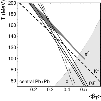
Figure 1: Relations between temperature and flow velocity extracted from hydrodynamical parameterizations of neutral pion spectra from WA98 (grey band) and from slope parameters of proton and antiproton (NA44 and NA49, solid lines), kaon (NA44, dashed lines) and deuteron spectra (NA44 and NA49, dotted lines). The light grey area shows the allowed region from pion interferometry analysis by NA49. (For details see text.)

The detailed analysis in [4] which obtains lower freeze-out temperatures uses additional information, namely the normalization of the spectra and two-particle correlations. It is known from other analyses (see e.g. [6]) that two-particle correlation which can provide constraints on $\left\langle\beta_{T}\right\rangle^{2}/T$ within hydrodynamical models effectively gives very little information on the temperature but constrains mostly the flow velocity (see light grey area in figure 1). On the other hand the normalization of spectra of different particle species is related to chemical freeze-out, while the spectral shape is influenced by kinetic freeze-out. To assume that these two corresponding temperatures are the same, as was apparently done in [4], is very likely wrong.

From the large pion-nucleon cross section one would assume that these two particle species are most likely to share the same freeze-out conditions. However, the influence of resonance decays in the pion spectrum forbids the simple use of slope parameters to estimate freeze-out conditions. To perform such a comparison the slope parameters for heavier particles will be used together with a full hydrodynamical parameterization of neutral pion spectra as described in [9]. The hydrodynamical computer program described in [10] has been modified to describe neutral pions and accommodate a Woods-Saxon density profile in addition to the default Gaussian profile and was used to obtain best parameter sets for $T$ and $\left\langle\beta_{T}\right\rangle$. The $2\sigma$-allowed values obtained for different profiles (Gaussian and Woods-Saxon of different diffuseness) are shown in figure 1 as a grey band. Among these fits, those obtained with large diffuseness (as e.g. the Gaussian) tend to yield smaller flow velocities for the same temperature but also constrain the allowed parameters to the high $T$ region [9]. In addition, the slope parameters for kaons, protons, antiprotons and deuterons from NA44 and NA49 as summarized in table 1 have been used with the help of equation 2 to obtain similar relations between $T$ and $\left\langle\beta_{T}\right\rangle$. All these estimates are also displayed in figure 1.

The NA49 collaboration has also published freeze-out constraints obtained from negative hadron and deuteron transverse mass spectra [6]. The negative hadrons are dominated by pions which should allow to use them in hydrodynamical descriptions assuming the pion mass, however, the analysis was performed using a non-relativistic approximation and ignoring resonance production. The deuteron spectra are not affected by resonances but still suffer from the non-relativistic approximation. The corresponding parameters are therefore not reliable. In fact, the estimate from the slope included in figure 1 differs considerably from the constraints in [6], esp. at large velocities. While the curves for kaons, protons and deuterons seem to converge around $T=140\,\mathrm{MeV}$ and $\left\langle\beta_{T}\right\rangle=0.33$, the neutral pion results have a further bias to somewhat higher temperatures. One should note that the analysis of the pion spectra differs from the others, as

1. a full parameterization including the effects of resonance decays has been performed compared to using an effective slope together with an approximate relation connecting $T$ and $\left\langle\beta_{T}\right\rangle$ and

2. they cover a different $m_{T}$ range – the high $m_{T}$ tail of the neutral pion spectrum has also been used as an upper limit as described in [9].

Still this figure suggests that a common parameter set for all the momentum spectra considered here can only be obtained for $T\geq 135\,\mathrm{MeV}$ and $\left\langle\beta_{T}\right\rangle\leq 0.35$. This appears to contradict constraints obtained from pion interferometry measurements [6] (see light grey area in figure 1), which favor larger transverse flow velocities.

2.2 Interferometry

It is well known that correlations between position and momentum space modify the radii measured in pion interferometry. One of the most interesting examples of such a correlation is collective flow [14, 15], both longitudinal and transverse, although there are other examples, like a source with local temperatures $T=T(x^{\mu})$, as I will discuss below. In the idealized case of pure collective motion (no thermal contribution) only the source element moving towards the detector will be measured, so the radius extracted from interferometry will correspond to this small elementary volume. If there is additional thermal motion, the probability of a particle to still be measured while being radiated from another source element at another space point and directed slightly away from the detector will increase. The effective source size will therefore decrease, if the amount of collective motion relative to thermal motion is large, and vice versa. In addition, this effect is a function of the momentum of the particle, and in most scenarios the effective radii will decrease with increasing transverse mass of the particle.

Most quantitative studies of these effects start from the Cooper-Frye formula [16] for the momentum distribution of the source:

$$E\frac{d^{3}N}{dp^{3}}=\frac{2J+1}{(2\pi)^{3}}\int_{\Sigma}d^{3}\sigma_{\mu}\frac{p^{\mu}}{\exp\left\{\left[p_{\mu}v^{\mu}-\mu\right]/T\right\}\mp 1}.$$ (4)

In this formula the factor $p^{\mu}$ in the numerator and the exponent $p_{\mu}v^{\mu}-\mu$ originate from the Lorentz transformation with $v^{\mu}=v^{\mu}(x^{\mu})$ being the local four-velocity of the source elements. In general also $T$ is again a local variable. $\mu$ is the chemical potential and the $\mp$ signs are relevant for bosons and fermions, resp.

There has been substantial work on extracting expressions for observables in interferometry, the most systematic approach using a parameterization of the source distribution and a saddle point approximation to extract approximate analytic relations for the effective radii [17]. A relatively general result is obtained using a source distribution expressed as:

$$S(x,K)=\frac{m_{t}\,{\rm ch}(\eta-Y)}{(2\pi)^{3}\sqrt{2\pi(\Delta\tau)^{2}}}\exp\left[-\frac{K{\cdot}u}{T}-\frac{x^{2}+y^{2}}{2R_{G}^{2}}-\frac{(\tau-\tau_{0})^{2}}{2(\Delta\tau)^{2}}-\frac{\eta^{2}}{2(\Delta\eta)^{2}}\right].$$ (5)

Gaussians are used for the space-time and rapidity distributions, the momentum spectrum is approximated as a Boltzmann distribution:

$$E\frac{d^{3}N}{dp^{3}}\propto\exp\left(-\frac{K{\cdot}u}{T}\right).$$ (6)

For a model with transverse expansion, the authors obtain approximate relations for the transverse and longitudinal radii:

$$R_{T} \approx R_{G}\left[1+\frac{m_{T}\beta_{T}^{2}}{T}{\rm ch}(\bar{\eta}-Y)\right]^{-1/2}$$ (7)

$$R_{L} \approx \tau_{0}\left[\frac{m_{T}}{T}{\rm ch}(\bar{\eta}-Y)-\frac{1}{{\rm ch}^{2}(\bar{\eta}-Y)}+\frac{1}{(\Delta\eta)^{2}}\right]^{-1/2}.$$ (8)

For a boost invariant longitudinally expanding source the expressions are more simple, e.g. for the longitudinal radius one obtains:

$$R_{L}\approx\tau_{0}\sqrt{\frac{T}{m_{T}}}.$$ (9)

As it turns out [6] that the source rapidity and the pair rapidity are similar $\bar{\eta}\approx Y$, also the expression for the transverse radius may be simplified:

$$R_{T}\approx R_{G}\left[1+\frac{\beta_{T}^{2}}{T}\cdot m_{T}\right]^{-1/2}.$$ (10)

These two latter equations are mostly used to extract information from experimental two-particle correlation functions. There are a number of assumptions which have to be made to obtain equations 7 and 8 and even more for equations 9 and 10. Some of these are discussed in [17], however there are further assumptions which I will try to concentrate on here.

To be able to use equation 10 to extract $\beta_{T}^{2}/T$ as in [6], one of the major assumptions is that the parameter $R_{G}$, which contains information on the geometrical size of the source, does not depend on the transverse momentum of the emitted particles. This is not necessarily correct. In general, there will not be a universal value for the temperature, it will be a local parameter depending on the position of the source element with respect to the center or the surface as discussed above.

This induces an additional correlation between momentum and coordinate space. If the variations in $T$ are very strong, this would of course invalidate all the attempts to extract the freeze-out temperature. If the variations are relatively weak, it may still be reasonable to use one effective temperature. It may e.g. be used to characterize momentum spectra, as for those the spatial distribution and therefore also these correlations are not directly relevant.

However, they are crucial to the analysis of pion interferometry, especially to the above mentioned method of extracting $\beta_{T}^{2}/T$. Consider e.g. that a certain fraction of pions is emitted before freeze-out, from the surface of the source, and that this fraction increases with increasing momentum. One might try to describe this with a superposition of two sources. Just as one example one may consider the following – arbitrary – scenario: One source of effective size (Gaussian) $R_{1}=10\,\mathrm{fm}$ and temperature $T_{1}=200MeV$ and a second with $R_{2}=2\,\mathrm{fm}$ and $T_{2}=400MeV$. If one investigates produced particles in different intervals of transverse mass, the relative contributions of these two sources will change, and implicitly the effective source size as seen in interferometry. This is shown in figure 2, where the effective source size – again approximated by a Gaussian – is shown as a function of the transverse mass for the case where the two sources discussed above both contribute the same fraction to the total multiplicity of particles. It can be seen easily that the effective source size decreases significantly with increasing transverse mass. Of course, this scenario has not been derived from physical arguments here, so it should only serve as an illustration of possible effects of such correlations between momentum and coordinate space. How large such effects might be would require a detailed model calculation which is not the scope of this paper. One should only note that in general $R_{G}$ in equation 7 is expected to be a function of $m_{T}$ within the model used. Values of $\beta_{T}^{2}/T$ should therefore be considered as upper limits unless more detailed model comparisons are performed. Pion interferometry is much more sensitive to such effects than momentum spectra.

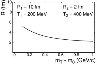
Figure 2: Effective source size as a function of the transverse mass of the particle for a superposition of two different sources (see text).

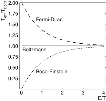
Figure 3: Inverse slopes (equation 11) relative to pure exponential slopes as a function of energy for different distribution functions.

A more fundamental caveat to the use of the $m_{T}$ dependence of HBT to estimate freeze-out parameters relates to another approximation used in extracting the analytical formula which are applied in most of the analyses. Specifically, the authors of [17] use the Boltzmann approximation to the distribution function. While this may be a good approximation for most of the pions used in experimental HBT analyses, it is well known that the deviations to the true Bose-Einstein distributions are crucial at low momenta. This is illustrated in figure 3, where the inverse slopes

$$T_{eff}=-\left[\frac{d}{dE}\log f(E)\right]^{-1}$$ (11)

of Bose-Einstein and Fermi-Dirac distributions

$$E\frac{d^{3}N}{dp^{3}}\propto\frac{1}{\exp\left(-\frac{E}{T}\right)\mp 1}.$$ (12)

are shown. Strong deviations from Boltzmann behaviour are seen for both distributions for $E/T<1$.

As in the analyses in question most of the $m_{T}$ dependence is seen at relatively low momenta, one should carefully reinvestigate the interpretation of these data with the correct statistical distributions. The trend of such a corrected analysis may be guessed from the behaviour of the slopes. Using the crude assumption that the BE-distributions may be locally approximated by a Boltzmann distribution, one might then use the formalism developed in [17] to estimate the $m_{T}$ dependence. However, now the effective slope for a Bose-Einstein distribution ($T_{BE}$) as shown in figure 3 should be used instead of the Boltzmann temperature $T$. In figure 4 the transverse radii as a function of transverse mass are shown for three different estimates:

1. Following the formalism as in [6], i.e. using the Boltzmann-like temperature in equation 10 and the results obtained in the article, i.e. $T=120\,\mathrm{MeV}$, $\left\langle\beta_{T}\right\rangle=0.55$ and $R_{G}=6.5\,\mathrm{fm}$,

2. substituting the temperature by the corresponding effective slope of a Bose-Einstein distribution, but using the same parameters as above and

3. substituting the temperature by the corresponding effective slope of a Bose-Einstein distribution, but now using $T=85\,\mathrm{MeV}$, $\left\langle\beta_{T}\right\rangle=0.55$ and $R_{G}=7.1\,\mathrm{fm}$.

It can be seen from this example that cases 1 and 2 show significant differences, and that for a rough agreement with 1 the temperature in the corrected version has to be modified from 120 MeV to 85 MeV as in case 3.

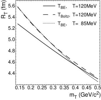
Figure 4: Transverse radii for pion interferometry as a function of transverse mass according to equation 10. The dashed line uses the Boltzmann temperature with values of $T=120\,\mathrm{MeV}$ and $\left\langle\beta_{T}\right\rangle\leq 0.55$, following the results of [6]. The solid line uses the same parameters with a correction for the effective slope of a Bose-Einstein distribution. The same correction is used for the dotted line but $T=85\,\mathrm{MeV}$ is assumed.

In this context it is interesting to investigate also results for proton source sizes. While the mechanism generating the correlation of particle pairs is different compared to pions – a strong interaction quasi-resonance instead of Bose-Einstein statistics, the picture of effective source sizes modified by the interplay of random thermal and collective hydrodynamical motion remains valid. People have therefore applied similar ideas to pp-correlation radii. The experiments NA49 [19] and NA44 [20] have measured proton correlations at midrapidity in Pb+Pb collisions - they obtain Gaussian radii in the range of $R_{pp}=3.5-4.0\,\mathrm{fm}$ which are considerably smaller that those extracted from pion interferometry ($R_{\pi\pi}=6-7\,\mathrm{fm}$). Similar values have been estimated by applying coalescence models to measured proton and deuteron multiplicities [20]. The smaller effective radii have been attributed to the much larger transverse mass of the protons, if a scaling with $1/\sqrt{m_{T}}$ which may be derived as an approximation from equations 9 and 10 is used for both protons and pions.

From the above argument on BE-distributions it is obvious that equivalent modifications are important here. However, the effective slope for a FD-distribution is larger at low momenta. In addition, the exponent of the FD-distribution contains a non-vanishing chemical potential which makes it much more likely that the exponent is small and that modifications are important.

Actually, another important argument is relevant here. If, as commonly believed, chemical freeze-out occurs relatively early before kinetic freeze-out, the relevant picture for the latter is the canonical ensemble, as the particle number for each species is fixed, so that there is no chemical potential as a parameter. The relevant energy in the statistical distributions is the kinetic energy and not the total energy, as no new particles are produced and the ground state energy of each particle is the rest mass. The Cooper-Frye formula should then be changed to:

$$E\frac{d^{3}N}{dp^{3}}=\frac{2J+1}{(2\pi)^{3}}\int_{\Sigma}d^{3}\sigma_{\mu}\frac{p^{\mu}}{\exp\left\{\left[p_{\mu}v^{\mu}-m_{0}\right]/T\right\}\mp 1}.$$ (13)

The major change for the transverse degrees of freedom would be to use $m_{T}-m_{0}$ instead of $m_{T}$. This should hold for both bosons and fermions, but while it might have only small effects on the pions, it will be dramatic for protons because of their large mass. It is beyond the scope of this paper to estimate the effect of such modifications on the $m_{T}$ spectra in general or, more specific, on the $m_{T}$ dependence of proton source sizes. However, it is also premature to conclude that proton and pion source sizes are compatible without performing detailed calculations. As the values of $m_{T}-m_{0}$ for protons and pions are roughly similar in the experiment, no difference in the radii would be expected between protons and pions from their transverse masses. This would however contradict the measured source sizes.

3 Conclusion

I have tried to illustrate above that the freeze-out parameters in ultrarelativistic heavy ion collision are not well established quantitatively. One should be careful to use only data sets which very likely share the same conditions. Also, the used approximations should be thoroughly investigated. The simple re-analysis of some of the available data performed here indicates the following:

• Transverse momentum spectra of deuterons, protons, kaons and pions seem to indicate that compatible parameter sets can be obtained only for $T\geq 135\,\mathrm{MeV}$ and $\left\langle\beta_{T}\right\rangle\leq 0.35$.

• The $m_{T}$ dependence of interferometry radii has to be reinvestigated using true statistical distributions instead of Boltzmann approximations at low momenta. This would also require to study the role of modifications related to the change at chemical freeze-out to a system with fixed particle number.

• Other possible sources of correlations between momentum and coordinate space may cause further alterations of the $m_{T}$ dependence of interferometry radii.

• The difference in pion and proton source sizes is very likely not explained by the difference in transverse mass of the two particles.

The three last observations shed doubt on the use of pion interferometry as the main ingredient to obtain constraints on the amount of transverse flow at freeze-out. A more thorough analysis of the pion interferometry results is necessary to clarify the situation.

Two possible scenarios may be envisaged which explain the data discussed here:

1. Pion HBT does not yield reliable constraints on kinetic (thermal) freeze-out. It may actually be that pion interferometry measures a different, later time than proton correlations and momentum spectra. This late “wave function freeze-out” may be related e.g. to very soft or mean field interactions of pions which do not alter the momentum distributions as mentioned in [21]. Momentum spectra, however, favour $T\geq 135\,\mathrm{MeV}$ and $\left\langle\beta_{T}\right\rangle\leq 0.35$.

2. Freeze-out does not occur with one even approximately universal temperature for different species and also different parts of the source.

Table 1: Parameters from transverse mass spectra of pions, kaons and protons in central 158$A$GeV Pb+Pb collisions. The slope parameters were taken from [3, 13, 11, 12], the average transverse momentum has been calculated assuming an exponential shape of the $m_{T}$ spectra in the fit range used.

particle		$T_{\rm eff}$ (MeV)	$\left\langle p_{T}\right\rangle$ (MeV)
$\pi^{+}$	NA44	$156\pm 6$	$531$
$\pi^{-}$	NA44	$154\pm 8$	$530$
$K^{+}$	NA44	$234\pm 6$	$556$
$K^{-}$	NA44	$235\pm 7$	$557$
$p$	NA44	$289\pm 7$	$705$
$\bar{p}$	NA44	$278\pm 9$	$695$
$p-\bar{p}$	NA49	$308\pm 15$	$720$
$d$	NA44	$376\pm 17$	$1115$
$d$	NA49	$376\pm 37$	$1069$

References

- [1] Quark Matter ’97, Proceedings of the 13th International Conference on Ultrarelativistic Nucleus-Nucleus Collisions, Tsukuba, Japan, Nucl. Phys. A 638 (1997).
- [2] Quark Matter ’99, Proceedings of the 14th International Conference on Ultrarelativistic Nucleus-Nucleus Collisions, Torino, Italy, Nucl. Phys. A 661 (1999).
- [3] NA44 Collaboration, I.G. Bearden et al., Phys. Rev. Lett. 78 (1997) 2080.
- [4] J.R. Nix et al.,nucl-th/9801045.
- [5] J.R. Nix, Phys. Rev. C 58 (1998) 2303.
- [6] NA49 Collaboration, H. Appelshäuser et al., Eur. Phys. J. C 2 (1998) 661–670.
- [7] A. Ster, T. Csörgö and J. Beier, Heavy Ion Phys, 10 (1999) 85-112.
- [8] A. Ster, T. Csörgö and B. Lörstadt, Nucl. Phys. A 661 (1999) 419c-422c.
- [9] WA98 Collaboration, M.M. Aggarwal et al., Phys. Rev. Lett 83 (1999) 926.
- [10] U.A. Wiedemann and U. Heinz, Phys. Rev. C 56 (1997) 3265.
- [11] NA49 Collaboration, H. Appelshäuser et al., Phys. Rev. Lett. 82 (1999) 2471-2475
- [12] NA49 Collaboration, H. Appelshäuser et al., Nucl. Phys. A 638 (1998) 91c-102c.
- [13] NA44 Collaboration, I.G. Bearden et al., Nucl. Phys. A 661 (1999) 55c-64c.
- [14] A. M. Makhlin and Yu. M. Sinyukov, Z. Phys. C 39 (1988) 69.
- [15] Yu. M. Sinyukov, Nucl. Phys. A 498 (1989) 151.
- [16] F. Cooper and G. Frye, Phys. Rev. D 10 (1974) 186.
- [17] S. Chapman, J.R. Nix and U. Heinz, Phys. Rev. C 52 (1995) 2694.
- [18] U. Heinz, Phys. Lett. B 382 (1996) 181.
- [19] NA49 Collaboration, H. Appelshäuser et al., Phys. Lett. B 467 (1999) 21-28.
- [20] NA44 Collaboration, I.G. Bearden et al., Nucl. Phys. A 661 (1999) 456c-459c.
- [21] S. Bass and A. Dumitru, Phys. Rev. C 61 (2000) 064909.