Mixing of the $f_{0}$ and $a_{0}$ scalar mesons in threshold photoproduction

Abstract

We examine the photoproduction of the light scalar mesons $f_{0}$-$a_{0}(980)$ with emphasis on isospin-violating $f_{0}$ and $a_{0}$ mixing due to the mass difference between neutral and charged kaons. General forms for the invariant amplitude for scalar meson photoproduction are derived, which yield expressions for the invariant mass distribution of the final meson pairs. A final state interaction form factor is obtained which incorporates $f_{0}$ and $a_{0}$ mesons, $K\bar{K}$ threshold effects, and $f_{0}-a_{0}$ mixing. This form factor is applied to predict the effective mass distribution of the $\pi\pi$ and $K\bar{K}$ pairs in the vicinity of the $K\bar{K}$ threshold. An estimate of the role of isospin mixing near threshold is provided. The potential role of polarized photons and protons is also discussed.

I Introduction

The $f_{0}$ and $a_{0}$ scalar mesons present a well-known puzzle for which several interesting, albeit controversial proposals have been made ranging from quark-antiquark makeup, to four-quark, and to $\bar{K}K$ molecular structure. Our goal is not to review these suggestions, but rather to investigate if new information on the makeup of these scalar mesons can be gleaned from threshold $f_{0}(980)$ and $a_{0}(980)$ photoproduction. Our hope is that threshold production of $0^{+}$ $K\bar{K}$ and two pion states that arise from the decay of scalar mesons will shed light on the nature of the $f_{0}$ and $a_{0}$ scalar mesons. For that purpose, we examine a potentially important final state isospin mixing effect.

The $f_{0}$ has been observed in a photoproduction experiment at Fermilab [2]. Measurements of exclusive $f_{0}$ photo/electroproduction are being performed at Jefferson Laboratory [3]. Extensive theoretical studies of $f_{0}$ photoproduction have been presented in recent papers [4, 5]. Our study differs from these works in that we assume $f_{0}$ and $a_{0}$ mesons are produced directly and play the role of doorway states, while in [4, 5] these mesons enter via final state interaction in $K\bar{K}$ and $\pi\pi$ channels. The two descriptions are complementary and further studies are needed to clarify their interconnection. Another novel feature of our present work is the inclusion of possibly important final state $f_{0}-a_{0}$ mixing. This mixing is induced by scalar meson transitions into and out of $K^{+}K^{-}$ and $K^{0}\bar{K}^{0}$ intermediate states, which generates $f_{0}-a_{0}$ mixing because of the 8 MeV splitting between the $K^{+}K^{-}$ and $K^{0}\bar{K}^{0}$ thresholds. Thus scalar meson mixing arises from the difference between the neutral and charged kaon masses, e.g. from isospin breaking. This effect is fully included into our treatment. Calculations presented below rely on a very restricted number of parameters and most of which are fixed using recent experimental data on the $\phi\rightarrow\gamma f_{0}/a_{0}$ reaction [6, 7] .

We study the reaction

$$\gamma+p\to p^{\prime}+f_{0}/a_{0}\to p^{\prime}+m_{1}m_{2}\ ,$$ (1)

using the $f_{0}$ and the $a_{0}$ as the possible doorway for subsequent decay meson production. Here $m_{1}m_{2}$ denotes $\pi\pi$ or $K\bar{K}$ pairs, or the $\pi\eta$ system. A thorough theoretical investigation of this reaction should include at least three essential points:

a) the general structure of the invariant scalar meson photoproduction amplitude, including expressions for the cross sections and spin observables;

b) effects of the final state interaction, including $K\bar{K}$ threshold phenomena;

c) a dynamical model for the reaction mechanism, e.g., an effective Lagrangian and/or a set of leading diagrams. In our paper we concentrate on points (a) and (b), which are more universal and less model dependent than point (c) above. The structure of the basic production amplitude and spin observables presented below do not rely on any explicit reaction mechanisms (other than the doorway assumption) and are applicable to the photoproduction of any scalar meson. The final state interaction (FSI) form factor we present later is constructed in a model independent way based on a theory of resonance mixture. Only a few parameters are needed which on one hand are sensitive to the nature of the $f_{0}/a_{0}$ mesons, and on the other can be extracted from recent experimental data on the $\varphi\rightarrow\gamma f_{0}/a_{0}$ reaction[6, 7]. Concerning the dynamical point (c), the dominant reaction mechanism is expected to depend upon the kinematical conditions of the explicit experiment. For example, at low photon momenta $s$–channel resonances might give a substantial contribution [8], while forward photoproduction at higher energies might be dominated by $t$–channel, $\rho$ and $\omega$ meson exchanges [4]. An alternate, very promising approach making use of chiral Lagrangians was proposed recently [5]. Although we do not propose an explicit reaction mechanism, our driving idea is complementary to that of Refs. [4, 5]. We take the $f_{0}/a_{0}$ to be “doorway states” for the reaction. Namely, we assume that $f_{0}/a_{0}$ scalar mesons are produced “directly” and then propagate under the strong influence of two nearby $K\bar{K}$ thresholds before decaying into $K\bar{K},\pi\pi,$ or $\pi\eta.$ This propagator, or FSI form factor, has a simple form and is applicable to any reaction involving $f_{0}/a_{0}.$

We begin by analyzing the structure of the photoproduction of scalar mesons using this $0^{+}$ doorway model, then we formulate a description of the final state interaction. The general behavior of the cross-section as a function of the invariant mass of the kaon or pion pair is then generated to gauge the importance of the mixing near threshold and for comparison with experiment. Speculations about the role of scalar-meson nucleon P-waves are presented, especially as they relate to the possible observation of spin observables.

II Diagrams and cross sections

Before focusing on $f_{0}/a_{0}$ photoproduction in reaction ( 1), we comment on possible background effects.

The amplitude for two-meson photoproduction $\gamma p\to p^{\prime}m_{1}m_{2}$ can be represented symbolically by the series of graphs depicted in Fig. 1. Although all diagrams entering into the background term $B_{\alpha}$  (Fig. 2) might be explicitly calculated (some of them were calculated in [4]), our main point is that $B_{\alpha}$ is a smooth function of the energy in the vicinity of the $K\bar{K}$ threshold; whereas, dramatic energy dependent effects in the invariant mass distribution of the $m_{1}m_{2}$ pair (see below) are generated mainly by the first two diagrams in Fig. 1. We neglect the pion loop diagram shown in Fig. 3 (see [4, 5])for two reasons. One reason is that near the $K\bar{K}$ threshold the pion loop by itself, i.e., without adding a resonant rescattering vertex, has smooth energy behavior and has to be included into the renormalized vertex of the $f_{0}$ production. The second reason for neglecting pion loops is based on Weinberg’s power counting theorem [9], which states that pion loops are suppressed compared to the tree diagrams depicted in Fig. 1. According to these arguments the pion loops are of the same order as higher terms in the effective Lagrangian. However, the above reasoning is far from being a rigorous proof of the direct production dominance. The theoretical and experimental study of this problem is at an early stage and we hope that comparison of complementary approaches will advance the investigation.

Consider now the graphs on the top of Fig. 1. We first consider only the $f_{0}$-meson; $a_{0}$ production will be included later. Then these diagrams under consideration are described by the following equation

$$T_{\alpha}=V_{\alpha f}G_{f}F_{f}+B_{\alpha},$$ (2)

where $F_{f}$ is the $f_{0}$ photoproduction amplitude, $G_{f}$ is the $f_{0}$ propagator (also called the FSI form factor), and $V_{\alpha f}$ is the amplitude for $f_{0}$ decay into the final meson pair channel $\alpha$ ($\alpha\equiv\pi\pi,K\bar{K}$), $B_{\alpha}$ denotes the background terms for channel $\alpha$ which we presume to be weakly energy dependent.

As shown below, the form factor $G_{f}$ contains dynamical information on the nature of the $f_{0}$ meson. This form factor also reflects the interplay of the $f_{0}$ with the nearby $K\bar{K}$ threshold. The simple kinematical fact that $K^{+}K^{-}$ and $K^{0}\bar{K}^{0}$ thresholds are split by 8 MeV induces significant $f_{0}/a_{0}$ mixing, as first noticed by Achasov et al. [10]. Taking account of this $f_{0}/a_{0}$ mixing, Eq. (2) is now extended to include a sum over intermediate $f_{0}$ and $a_{0}$ states

$$T_{\alpha}=\sum_{i,k}\ V_{\alpha i}G_{ik}F_{k}+B_{\alpha},$$ (3)

with $i,k=f_{0},a_{0}$, i.e., the form factor $G_{ik}$ becomes a $2\times 2$ matrix in $f_{0}/a_{0}$ space. As pointed out earlier by Stodolsky [12] measurement of the invariant mass distribution of the $(m_{1}+m_{2})$ system in reaction ( 1) enables one to determine the nonorthogonality of the decaying states; i.e. the probability for $f_{0}\leftrightarrow a_{0}$ transitions.

The cross section for the reaction $\gamma p\to p^{\prime}m_{1}m_{2}$ (see Fig. 1), where the meson pair is in channel $\alpha,$ is

$$\sigma_{\alpha}=\frac{m^{2}}{(2\pi)^{3}}\frac{1}{\lambda^{1/2}(s,0,m^{2})}\int dE_{m_{1}}\ dE_{m_{2}}\ \frac{d\Omega_{m_{1}}}{4\pi}\ \frac{d\varphi_{m_{2}}}{2\pi}\ |T_{\alpha}|^{2},$$ (4)

where $\lambda(x,y,z)\equiv(x-y-z)^{2}-4yz,\ s=(k+p)^{2}=(p^{\prime}+q_{m_{1}}+q_{m_{2}})^{2},\ m$ is the proton mass, $\Omega_{m_{1}}$ is the angle of decay meson 1 with respect to the incident photon beam $\vec{k}$ and $\Omega_{m_{2}}=(\cos\theta_{m_{1}m_{2}},\varphi_{m_{2}})$ is the angle of decay meson 2 with respect to $\Omega_{m_{1}}$. The decay mesons are coplanar as described by $\varphi_{m_{2}}.$

To observe the $f_{0}/a_{0}$ meson and to investigate its properties use is made of the double differential cross section

$$\frac{d\sigma_{\alpha}}{dt\ dm_{x}}=\frac{m^{2}}{(2\pi)^{3}}\ \frac{\sqrt{\lambda(m^{2}_{x},m^{2}_{m_{1}},m^{2}_{m_{2}})}}{4\ m_{x}\ \lambda(s,0,m^{2})}\ \frac{1}{4\pi}\ \int d\Omega^{*}\ |T_{\alpha}|^{2},$$ (5)

or of the invariant mass $m_{x}$ distribution

$$\frac{d\sigma_{\alpha}}{dm_{x}}=\frac{m^{2}}{(2\pi)^{3}}\ \frac{\sqrt{\lambda(s,m^{2}_{x},m^{2})\ \lambda(m^{2}_{x},m^{2}_{m_{1}},m^{2}_{m_{2}})}}{4\ s\ m_{x}\ (s-m^{2})}\frac{1}{2}\int^{+1}_{-1}d\cos\theta\ \frac{1}{4\pi}\ \int\ d\Omega^{*}\ |T_{\alpha}|^{2},$$ (6)

where $t=(p-p^{\prime})^{2},m_{x}=s^{1/2}_{1},s_{1}=(p_{m_{1}}+p_{m_{2}})^{2},$ and $\Omega^{*}$ is the angle between the relative momentum of the two decay mesons in their c.m. system. The angle $\theta$ refers to the scalar meson production angle. Proton spinors are normalized according to $\bar{u}u=1.$ We will use this last expression to display the cross-section as a function of the invariant mass $m_{x}$, once we have described the amplitude $T_{\alpha}$ of Eq. (3).

The initial and final helicity summations are suppressed above in $|T_{\alpha}|^{2}.$ For unpolarized beam, target and recoil proton experiments, it is therefore understood that one sums over final and averages over initial helicities. However, if one has a polarized beam or polarized target, the associated cross sections can be expressed, using the bold assumption that $B_{\alpha}$ interference can be neglected, by:

$$|T_{\alpha}|^{2}=V_{\alpha i}G_{ik}\ Tr[(F_{k}\rho_{I}F^{\dagger}_{k^{\prime}})]\ G^{*}_{i^{\prime}k^{\prime}}V^{*}_{\alpha i^{\prime}}\ ,$$ (7)

where $\rho_{I}$ is the density matrix which describes the spin state of the initial beam and target. Since the decay $V_{\alpha i}$ and the propagator $G_{ik}$ are both independent of helicities, the inner term above ${\cal S}_{kk^{\prime}}=Tr[(F_{k}\rho_{I}F^{\dagger}_{k^{\prime}})]$ includes a trace over the helicity quantum numbers in the usual way. The function ${\cal S}_{kk^{\prime}}$ is a coupled-channels version of the usual ensemble average expression. For a polarized recoil proton experiment, ${\cal S}_{kk^{\prime}}$ generalizes to ${\cal S}_{kk^{\prime}}=Tr[\rho_{F}(F_{k}\rho_{I}F^{\dagger}_{k^{\prime}})],$ where $\rho_{F}$ describes the final recoil polarization measurement. With this expression, it is possible to extract the effect of having a polarized beam and/or target on the cross-section. It is of interest to see if such measurements, especially as meson-nucleon P-waves appear, can shed light on the structure of the scalar mesons.

We are now ready to examine the structure of scalar meson photoproduction in order to specify the scalar meson production amplitude $F.$

III Invariant Amplitudes and Spin Observables for the Scalar Meson

The spin structure of the scalar meson photoproduction amplitude $F$ and the corresponding spin observables are discussed in this section. Again $k$, $p$ and $p^{\prime}$ denote the 4-momenta of the photon and the initial and final protons, respectively; while the scalar meson’s 4-momentum is denoted by $q.$ The decomposition of the scalar meson photoproduction amplitude as invariant amplitudes has the following (CGLN [13])form

$$F=\bar{u}(p^{\prime})\sum^{4}_{j=1}M_{j}A_{j}(s,t,u)u(p).$$ (8)

We follow the $\bar{u}u=1$ normalization conditions of [14]. For the scalar meson, the four invariant amplitudes $M_{j}$ are

$$M_{1}=-{\varepsilon\mkern-8.0mu\raise-0.43057pt\hbox{/}}{k\mkern-10.0mu\raise-0.43057pt\hbox{/}},$$

$$M_{2}=2(\varepsilon p)(kp^{\prime})-2(\varepsilon p^{\prime})(kp),$$

$$M_{3}={\varepsilon\mkern-8.0mu\raise-0.43057pt\hbox{/}}\ (kp)-{k\mkern-10.0mu\raise-0.43057pt\hbox{/}}\ (\varepsilon p),$$ (9)

$$M_{4}={\varepsilon\mkern-8.0mu\raise-0.43057pt\hbox{/}}\ (kp^{\prime})-{k\mkern-10.0mu\raise-0.43057pt\hbox{/}}\ (\varepsilon p^{\prime}),$$

where $\varepsilon_{\mu}$ is the photon polarization 4-vector. The four amplitudes $M_{i}$ differ from the $0^{-}$ meson photoproduction only in the omission of the $\gamma_{5}$ pseudoscalar factor.

The amplitude $F$ can be expressed in terms of the two–component spinors $\chi$. For this purpose we write

$$F=\sqrt{\frac{\omega(p)\omega(p^{\prime})}{4m^{2}}}<\chi(p^{\prime})|R|\chi(p)>,$$ (10)

where $\omega(p)=E_{p}+m$. Substitution of the invariant amplitudes Eq. (10) into Eq. (8) leads to the following CGLN-type representation for the amplitude $R$

$$R=i\vec{\varepsilon}\cdot(\vec{\sigma}\times\hat{k})\ {R_{1}}+(\vec{\varepsilon}\cdot\vec{\sigma})(\vec{\sigma}\cdot\hat{q})\ {R_{2}}+i(\vec{\varepsilon}\cdot\hat{q})(\hat{q}\times\hat{k})\cdot\vec{\sigma}\ {R_{3}}+(\vec{\varepsilon}\cdot\hat{q})\ R_{4}\ ,$$ (11)

where $\hat{k},\hat{q}$ are unit vectors. The four amplitudes $R_{j}$ are related to the four amplitudes $A_{j}$ of Eq. (8) via

$$R_{1}=-(\sqrt{s}-m)\Big{\{}A_{1}+\frac{1}{2}(\sqrt{s}-m)A_{3}+\frac{(kp^{\prime})}{\sqrt{s}+m}A_{4}\Big{\}}$$

$$R_{2}=\frac{|\vec{q}\,|}{E_{p^{\prime}}+m}\Big{\{}-(\sqrt{s}-m)A_{1}+\frac{1}{2}(s-m^{2})A_{3}+(kp^{\prime})A_{4}\Big{\}}$$ (12)

$$R_{3}=|\vec{q}\,|^{2}(\frac{\sqrt{s}-m}{E_{p^{\prime}}+m})\Big{\{}(\sqrt{s}-m)A_{2}-A_{4}\Big{\}}$$

$$R_{4}=-(\sqrt{s}-m)\ |\vec{q}\,|\ \Big{\{}A_{2}(\sqrt{s}+m)[1-\frac{\vec{k}\cdot\vec{q}}{(E_{p}+m)(E_{p^{\prime}}+m)}]+$$

$$+A_{4}[1+(\frac{\sqrt{s}+m}{\sqrt{s}-m})\frac{\vec{k}\cdot\vec{q}}{(E_{p}+m)(E_{p^{\prime}}+m)}]\Big{\}}.$$

The $(kp^{\prime})$ factor denotes a 4-vector product. To recast  (12) into a fully relativistic invariant form, the following simple kinematical equations may be used

$$2(\vec{k}\cdot\vec{q})=t-\mu^{2}+\frac{1}{2s}(s-m^{2})(s-m^{2}+\mu^{2}),$$

$$2kp^{\prime}=m^{2}-u,$$

$$|\vec{q}\,|=\frac{1}{2\sqrt{s}}\lambda^{1/2}(s,\mu^{2},m^{2}),$$ (13)

$$E_{p}=\frac{1}{2\sqrt{s}}(s+m^{2}),E_{p^{\prime}}=\frac{1}{2\sqrt{s}}(s+m^{2}-\mu^{2}),$$

where $\mu$ is the mass of either $f_{0}$ or $a_{0}.$ Note that an alternative form of the amplitude (12) may be found in Ref. [15].

Note that at the scalar meson production threshold all of the $R_{i}$ amplitudes vanish except for $R_{1}.$ We conclude that at the scalar meson production threshold the operator $F$ is given by

$$F=\frac{[\omega(p)\omega(p^{\prime})]^{1/2}}{2m}\ R_{1}\ i\vec{\varepsilon}\cdot(\vec{\sigma}\times\hat{k}).$$ (14)

The value of the coefficient $R_{1}$ is discussed below in Sec. 5.

As meson-nucleon P-waves turn on, the associated $J=\frac{1}{2}^{-},J=\frac{3}{2}^{-}$ amplitudes contribute with an initial linear dependence on the momentum $|\vec{q}\ |;$ hence, it is likely that the terms $R_{2}$ and $R_{4}$ will appear along with their operators. That unfolding of P-waves has implications concerning which spin observables assume nonzero values as the energy rises beyond the threshold value of $E_{\gamma}(lab)=1.5\$ GeV.

IV The Form Factor of the scalar Mesons near the $K\bar{K}$ Threshold

In this section, we consider the FSI form factors $G_{f}$(pure $0^{+}$ propagation) and $G_{ik}$(coupled $0^{+}$ propagation) introduced in (2) and (3). These form factors describe the propagator of an unstable particle in the energy region overlapping some of the decay thresholds ($K^{+}K^{-}$ and $K^{0}\bar{K}^{0}$). We are mainly interested in the coupled-channel form factor $G_{ik},$ which includes $f_{0}-a_{0}$ mixing, but to simplify the discussion, we start with the simple one-channel propagator $G_{f},$ which describes the $f_{0}$-meson and its decay channels. Later we generalize that discussion to the coupled-channels $G_{ik}$ case.

There exists an overwhelming number of approaches to describe an unstable particle and particle mixtures. We follow the general phenomenological approach developed by Stodolsky [16] and Kobzarev, Nikolaev and Okun [17], and in a slightly modified form presented in the book of Terent’ev [18]. This approach has already been applied to the $f_{0}/a_{0}$ system in [19]. We now briefly outline the derivation of the basic equations for propagation of an unstable particle; see [16, 17, 18, 19] for details.

First consider $f_{0}$ and its decay channels ($a_{0}$ will be incorporated later) and let us introduce a set of state vectors $\mid i>$ describing the scalar meson. One of these states, often denoted as $\mid f>,$ is a discrete state; continuum states are also included in the set $\mid i>.$ The discrete state couples to the continuum states and thereby acquires a width and a shift in mass; e.g., it becomes an unstable state. Let the whole scalar meson system be described by the Hamiltonian $H=H_{0}+V$, where $H_{0}$ has a multichannel continuous spectrum $H_{0}\mid i>=E_{i}\mid i>$ and a discrete state $H_{0}\mid f>=E_{f}\mid f>.$ The interaction V is responsible for the transitions between the above channels, so that with V “turned on,” $\mid f>$ becomes a resonance. Consider the transition amplitude

$$A_{if}(t)\equiv<i\mid f;t>,$$ (15)

where $\mid f;t>=\exp(-i(H_{0}+V)t)\mid f>$. “Diagonal” transitions $A_{ff}(t)$ are also included in this definition. The amplitude $A_{if}(t)$ satisfies the equation

$$i\frac{\partial}{\partial t}A_{if}(t)=E_{i}\ A_{if}(t)+\sum_{j}\ V_{ij}\ A_{jf}(t),$$ (16)

where $V_{ij}=<i\mid V\mid j>,$ and the initial condition is $A_{if}(0)=\delta_{if}$. The equivalent integral equation reads

$$A_{if}(t)=e^{-iE_{i}t}A_{if}(0)-i\ \sum_{j}\int^{t}_{0}dt^{\prime}\ V_{ij}\ e^{-iE_{i}(t-t^{\prime})}A_{jf}(t^{\prime}).$$ (17)

Next we introduce the propagator for the interacting scalar meson system in the energy representation

$$G_{if}(E+i\delta)=\int^{\infty}_{0}dt\ e^{i(E+i\delta)t}A_{if}(t).$$ (18)

Applying a time integration similar to Eq. (18) to all of Eq. (17) yields

$$G_{if}(E+i\delta)=\frac{iA_{if}(0)}{E-E_{i}+i\delta}+\sum_{j}V_{ij}\ \frac{G_{jf}(E+i\delta)}{E-E_{i}+i\delta}.$$ (19)

For $i\neq f$ taking account of the initial condition, one gets

$$G_{if}(E+i\delta)=V_{if}\ \frac{G_{ff}(E+i\delta)}{E-E_{i}+i\delta}+\sum_{j\neq f}V_{ij}\ \frac{G_{jf}(E+i\delta)}{E-E_{i}+i\delta}\ ,$$ (20)

while for $i=f$ the equation has the form

$$G_{ff}(E+i\delta)=\frac{i}{E-E_{f}+i\delta}+V_{ff}\ \frac{G_{ff}(E+i\delta)}{E-E_{f}+i\delta}+\sum_{j\neq f}V_{fj}\ \frac{G_{jf}(E+i\delta)}{E-E_{f}+i\delta}\ .$$ (21)

Now we return to  (20) and assume that $V$ only connects $|f>$ with its decay channels, while direct coupling between decay channels is absent, i.e., $V_{ij}=0$ in Eq. (20) (this assumption may be dropped without changing the results significantly see Ref. [16]). Then we take $G_{if}$ given by the left hand side of Eq. (20) with $V_{ij}=0$ on the right hand side, change the index $i$ in $G_{if}$ into $j$ and substitute this $G_{jf}$ into  (21). Thus we obtain

$$\Big{(}E-E_{f}-V_{ff}-\sum_{j\neq f}V_{fj}\ \frac{1}{E-E_{j}+i\delta}V_{jf}+i\delta\Big{)}G_{ff}(E+i\delta)=i.$$ (22)

This is the result for a pure $f_{0}$ meson case. The physical meaning of this propagator is that there is a shift in energy of the interacting meson due to a self interaction, plus a complex contribution from transitions to intermediate continuum states. Some of the flux into the intermediate state returns to the discrete state $|f>,$ some flows away, thereby creating a shift in the width as well as the real part of the energy. Note, we often designate the interacting propagator $G_{ff}$ simply as $G_{f}.$ We now examine the role of the scalar mesons coupling to pion and kaon pairs in the intermediate states.

Some remarks are now in order. Since we are interested in $K\bar{K}$ channels with thresholds close to the $f_{0}$ mass the non-relativistic derivation and in particular nonrelativistic kinematics used above are justified; the relativistic generalization is straightforward. Keeping in mind that $\pi^{+}\pi^{-}$ and $\pi^{0}\pi^{0}$ thresholds are far away from the $f_{0}$ position, we rewrite Eq. (22) in terms of “renormalized” eigenvalues instead of the “bare” ones. By that we mean that $E_{f}$ is redefined to include both the self-energy contribution $V_{ff}$ and the part of the sum in Eq. (22) that arises from channels other than the $K\bar{K}$ channels. Hence, effects of the $\pi^{+}\pi^{-}$ and $\pi^{0}\pi^{0}$ are incorporated by redefining or renormalizing $E_{f}.$ In the vicinity of the $K\bar{K}$ threshold, the terms arising from intermediate pion pairs are almost energy independent. They shift $E_{f}$ by the following real and imaginary parts

$$\sum_{\pi\pi}V_{f\pi\pi}\frac{1}{E-E_{\pi\pi}+i\delta}V_{\pi\pi f}=M_{f}-i\frac{\Gamma_{f}}{2}.$$ (23)

The width $\Gamma_{f}$ is thus generated by the imaginary part of the transitions to the pion pair continuum. For the $a_{0}$-meson propagator analogous real and imaginary energy shifts arise from $\eta\pi$ intermediate states. The sum in (23) implies both a sum over different channels ($\pi^{+}\pi^{-}$ and $\pi^{0}\pi^{0}$) and integration over the energies $E_{\pi\pi}$ in each channel. For large values of $E_{\pi\pi}$ the integral diverges and standard renormalization has to be performed. In the simplified approach presented here we may even argue that the integral is convergent (or cut off) due to the matrix elements $V_{f\pi\pi}$, $V_{\pi\pi f}$. We keep the same notation $E_{f}$ for the real part of the $f_{0}$ energy renormalized in the above sense; i.e., after $V_{ff}$ and $M_{f}$ are absorbed into it. Then the $f_{0}$ propagator takes the following simple form

$$G_{f}(E+i\delta)=\frac{i}{E-E_{f}+i\frac{\Gamma f}{2}-\sum_{K\bar{K}}V_{fK\bar{K}}\frac{1}{E-E_{K\bar{K}}+i\delta}V_{K\bar{K}f}}\ \ ,$$ (24)

where summation is now only over $K^{+}K^{-}$ and $K^{0}\bar{K}^{0}$ channels and the sum also implies integration over energy. Being interested in the $K\bar{K}$ near threshold energy region, one cannot neglect the splitting between $K^{+}K^{-}$ and $K^{0}\bar{K}^{0}$ thresholds equal to 2 ($m_{K^{0}}-m_{K^{\pm}})$ = 8 MeV. This mass difference induces isospin violating $f_{0}-a_{0}$ mixing. Such “kinematical” isospin violation was carefully studied earlier using effective range theory [20]. For the $f_{0}-a_{0}$ system the effect was probably first pointed out in [10], where it was shown that mixing is enhanced, i.e., is of the order of $[(m_{K^{0}}-m_{K^{\pm}}]/m_{K^{0}}]^{\frac{1}{2}},$ instead of $[(m_{K^{0}}-m_{K^{\pm}}]/m_{K^{0}}]$ as might be naively expected. As we shall see, this enhancement also follows in our approach and motivates us to include this effect in scalar meson production. Isospin violating $f_{0}-a_{0}$ mixing has also been studied earlier by T. Barnes. [11]

We will not repeat the derivation including the $a_{0}$ meson since it proceeds along the same lines. The propagator now becomes a $2\times 2$ matrix in the $f_{0}-a_{0}$ basis. Instead of  (22) and  (24), one gets

$$\sum_{m=f,a}\left[(E-E_{n}+i\frac{\Gamma_{n}}{2})\delta_{nm}-\sum_{K\bar{K}}V_{nK\bar{K}}\frac{1}{E-E_{K\bar{K}}+i\delta}V_{K\bar{K}m}\right]G_{mk}=i\delta_{nk},$$ (25)

where $n,k=f,a.$ The $a_{0}$-meson entering into this equation has been also “renormalized,” this time the $\pi\eta$ channel plays the role of the $\pi\pi$ channel for $f_{0}$.

Our next task is to present explicit expressions for the sums over $K\bar{K}$ entering into (24) and (25). This problem was considered in [19] in detail including the Coulomb interaction in the $K^{+}K^{-}$ channel. The Coulomb interaction results in spectacular effects including the formation of the $K^{+}K^{-}$ atom, but the typical energy scale for these phenomena is of the order of few KeV which requires an experimental resolution that is probably inaccessible in the near future. Neglecting the Coulomb interaction, the above sums are reduced to expressions of the type

$$\sum_{K\bar{K}}V_{nK\bar{K}}Y(m_{x},m_{K})V_{K\bar{K}m}\ ,$$

where we replaced $E$ by $m_{x}$ to be consistent with expressions (5-6) for the cross sections; here, $Y(m_{x},m_{K})$ are integrals of the type

$$Y(m_{x},m_{K})=\frac{1}{2m^{3}_{x}}\ \int\frac{d^{3}p}{(2\pi)^{3}}\frac{1}{m_{x}-2m_{K}-\frac{p^{2}}{m_{K}}+i\delta}\ \ \ ,$$ (26)

with $m_{K}=m_{K^{\pm}},m_{K^{0}}$. As already mentioned, the integral  (26) is formally divergent which is however neither dangerous or important as soon as we focus on the $m_{x}$ region close to the $K\bar{K}$ threshold. Close to the $K\bar{K}$ threshold the leading energy dependent contribution is

$$Y(m_{x},m_{K})=-i\frac{1}{32\pi m_{x}}\ \sqrt{\frac{m_{x}-2m_{K}}{m_{K}}+i0}\ ,$$ (27)

where $+i0$ means that for $m_{x}<2\,m_{K}$ the square root acquires a positive imaginary part. From ( 25) and ( 27), it follows that for $m_{x}>2\,m_{K}$ the decay width into the $K\bar{K}$ channel is given by $(n=f,a)$

$$\Gamma_{nK\bar{K}}=\frac{\mid V_{nK\bar{K}}\mid^{2}}{16\pi m_{x}}\sqrt{\frac{m_{x}-2m_{K}}{m_{K}}}\ .$$ (28)

Comparison of ( 28) with the parameterization used in [6] shows that $V_{nK\bar{K}}=g_{nK\bar{K}},$ where $g_{nK\bar{K}}$ are the coupling constants used in [6]. Recall that Eq. (25) is written in the basis of $f_{0}$ and $a_{0}$ states having definite isospins, $I_{f_{0}}=1,I_{a_{0}}=0.$ Therefore,

$$V_{K^{+}K^{-}f}=V_{K^{0}\bar{K}^{0}f}\ \ \,\ \ V_{K^{+}K^{-}a}=-V_{K^{0}\bar{K}^{0}a}\ .$$ (29)

Next we introduce the notation

$${\cal D}\equiv\frac{\mid V_{K^{+}K^{-}f}\mid^{2}}{32\pi m_{x}}\ \ ,\ \ \zeta\equiv\frac{V_{K^{+}K^{-}a}}{V_{K^{+}K^{-}f}}\ \ ,$$ (30)

where $\zeta$ can be complex with phase $\phi,$ see later. In this notation, the explicit form of Eq. (25) can be expressed as a matrix in $f_{0}-a_{0}$ space as:

$$i\hat{G}^{-1}=\bigg{(}\begin{array}[]{cc}m_{x}-E_{f}+i\frac{\Gamma_{f}}{2}&0\cr 0&m_{x}-E_{a}+i\frac{\Gamma_{a}}{2}\end{array}\bigg{)}$$ (33)

$$+i{\cal D}\bigg{(}\begin{array}[]{cc}1&\zeta\cr\zeta^{*}&|\zeta|^{2}\end{array})\bigg{)}\sqrt{\frac{m_{x}-2m_{K^{+}}}{m_{K^{+}}}+i0}$$ (36)

$$+i{\cal D}\bigg{(}\begin{array}[]{cc}1&-\zeta\cr-\zeta^{*}&|\zeta|^{2}\end{array}\bigg{)}\sqrt{\frac{m_{x}-2m_{K^{0}}}{m_{K^{0}}}+i0}\ \ ,$$ (39)

Here we see that the isospin violating $f_{0}-a_{0}$ mixing is really proportional to $\sqrt{\frac{m_{x}-2m_{K}}{m_{K}}}$ and is indeed enhanced as was pointed out in Ref. [10]. We also see that far beyond the region $|m_{x}-2m_{K}|\approx 8MeV$ of the $K\bar{K}$ thresholds, the nondiagonal elements cancel each other and thereby extinguish the $f_{0}-a_{0}$ mixing. Away from the threshold region one should also take into account corrections to ( 27), i.e., include the next terms in the expression for the renormalized kaon loop.

Now we have at our disposal all quantities needed to calculate the near threshold amplitudes and cross sections using equations presented in Sec. 2. For example, the amplitude for the process $\gamma+p\rightarrow p^{\prime}+f_{0}\rightarrow p^{\prime}+\pi\pi$ reads

$$T_{\pi\pi}=V_{\pi\pi f}G_{ff}F_{f}+V_{\pi\pi f}G_{fa}F_{a}+B_{\pi\pi}.$$ (40)

Here we see the doorway production of the $f_{0}$, followed by its subsequent propagation via $G_{ff}$ and then its decay $V_{f\pi\pi}.$ The second term includes the doorway production of the $a_{0},$ followed by its transition into a $f_{0}$ via isospin violation and then the $f_{0}$ decays into a pion pair. Other pion pair processes are included in the background term $B_{\pi\pi}.$ For final kaon production the corresponding result is:

$$T_{K^{+}K^{-}}=V_{K^{+}K^{-}f}\ G_{ff}\ F_{f}+V_{K^{+}K^{-}a}\ G_{aa}\ F_{a}+V_{K^{+}K^{-}f}\ G_{fa}\ F_{a}+V_{K^{+}K^{-}a}\ G_{af}\ F_{f}+B_{K^{+}K^{-}}\ \ .$$ (41)

For final $\pi\eta$ production the corresponding result is:

$$T_{\pi\eta}=V_{\pi\eta a}\ G_{aa}\ F_{a}+V_{\pi\eta a}\ G_{af}\ F_{f}+B_{\pi\eta}.$$ (42)

The values of the parameters are discussed in the next section.

V Parameters of the Model

The theoretical investigation of the light scalar mesons $f_{0}$ and $a_{0}$ has a long history. A most thoughtful study of $f_{0}/a_{0}$ has been performed by the Novosibirsk group (see [6, 7] and references therein). Although our approach differs from other authors, including the Novosibirsk group, the key parameters are similar in various treatments. Thus, in order to fix the parameters we shall relate them to those used by the Novosibirsk group. This would still leave the set of parameters incomplete, namely the photoproduction amplitude $F_{k}$ and the background term $B_{\alpha}$ ( see Eq.3) have no analogues in the Novosibirsk set and to get at least an educated guess about them, we resort to the recent paper [5]. We stress that the characteristics of $f_{0}/a_{0}$ are at present far from being perfectly established. For example, the Novosibirsk group presents several solutions with some of the parameters ranging over rather wide limits [6]. In order to determine the parameters of the model we use the recent experimental data presented in [7]. These data do not allow us to fix all the parameters and some parameters will be set from different consideration (see below).

The model under consideration can be described by several equivalent sets of parameters. We used the following set: $E_{f},E_{a},\Gamma_{f},\Gamma_{a},V_{fK^{+}K^{-}}$, and $\zeta$. The quantities $V_{fK^{0}\bar{K}^{0}}$, $V_{aK^{0}\bar{K}^{0}}$ and ${\cal D}$ are then expressed according to ( 29) and ( 30), while $V_{f\pi\pi}$ and $V_{a\pi\eta}$ are determined via $\Gamma_{f}$ and $\Gamma_{a}$ according to the equation

$$\Gamma_{jm_{1}m_{2}}=\frac{|V_{jm_{1}m_{2}}|^{2}}{16\pi m_{x}}\rho_{m_{1}m_{2}}\,,$$ (43)

where $j=f,a$, and $\rho_{m_{1}m_{2}}$ is the two-body phase space. At this point we remind the reader that since we treat the $K\bar{K}$ channels explicitly, their contribution does not enter into $E_{j}$ and $\Gamma_{j}(j=f,a)$. We also mention that the “visible” widths of $f_{0}/a_{0}$ are smaller than the widths $\Gamma_{f}$ and $\Gamma_{a}$ [6]. Finally, we recall that our parameters $V_{jm_{1}m_{2}}$ are equivalent to $g_{jm_{1}m_{2}}$ used by the Novosibirsk group [6] [7].

In [7] we find the following parameters relevant for our purposes (experimental errors are omitted):

$$\frac{|V_{f\pi\pi}|^{2}}{4\pi}=0.44\ GeV^{2}\;,R=\frac{|V_{fK\bar{K}}|^{2}}{|V_{f\pi\pi}|^{2}}=3.77\,.$$ (44)

Using ( 43) and isotopic relations

$$|V_{f\pi^{+}\pi^{-}}|^{2}=\frac{2}{3}|V_{f\pi\pi}|^{2},\ \ \ \ |V_{fK^{+}K^{-}}|^{2}=\frac{1}{2}|V_{fK\bar{K}}|^{2},$$ (45)

we get from ( 44):

$$\Gamma_{f}=0.1\ GeV\,,V_{fK^{+}K^{-}}=3.23\ GeV\,.$$ (46)

Next setting in ( 39) $m_{x}$ equal to the physical mass of the $f_{0}$-meson, i. e. $m_{x}=0.98$ GeV, we find $E_{f}=0.947$ GeV. Unfortunately, we can not rely on well-established experimental data for the parameters of the $a_{0}$ meson. Therefore we assume $\Gamma_{a}\equiv\Gamma_{f}$ and $E_{a}\equiv E_{f}$ (these assumptions are in line with the solutions proposed in [6].) From $\Gamma_{a}$ we get $V_{a\pi\eta}=3.08$ GeV. Finally we set $\zeta=1,$ which is true in both four-quark and molecular models of $f_{0}/a_{0}$ [6]. Thus we arrive at the following parameter set (set A):

$$E_{f}=E_{a}=0.947\ GeV,\;\Gamma_{a}=\Gamma_{f}=0.1\ GeV,\;\\ V_{fK^{+}K^{-}}=3.23\ GeV,\;\zeta=1.$$ (47)

Note that the value $|V_{fK^{+}K^{-}}|^{2}/4\pi=0.83$ GeV² lies in between the values typical for four-quark and molecular models of $f_{0}$-meson [6].

In order to display the effect of $f_{0}-a_{0}$ mixing, we consider also set B whose only difference from set A is that in B the splitting of the $K^{0}\bar{K}^{0}$ and $K^{+}K^{-}$ thresholds is ignored and the kaon mass is taken equal to the average value $m_{K}=\frac{1}{2}(m_{K^{0}}+m_{K^{\pm}})$ and hence mixing is thereby turned off. This results in cancellation of the non-diagonal terms in Eq. 39.

Within our approach we are not in a position to determine the value of the photoproduction amplitude $F_{j}(j=f,a).$ Its invariant structure is given by Eqs. 9 and  11, but the magnitudes of the invariant amplitudes remain unknown. In a recent paper [5] the $f_{0}/a_{0}$ photoproduction has been considered in the near-threshold region, namely at $k=1.7\ GeV.$ Close to threshold the dominant contribution stems from the amplitude $R_{1}$ of Eq. 11. Its value can be considered a free parameter, but we prefer to take for $R_{1}$ the value proposed in [5].  The reasons for adopting this value for $R_{1}$ is on one hand because it enables a direct comparison of our results with that of [5] and on the other hand, as already argued in Sec. 2, we may consider the pion loops included into the renormalized vertex of $f_{0}$ photoproduction while in the approach of [5] the two pion photoproduction is the driving mechanism that determines the value of $R_{1}.$

The calculation or even estimate of the background term $B_{\alpha}$ in  2 is beyond the scope of this article. Some of the diagrams entering into $B_{\alpha}$ are depicted in Fig. 2 and in general may be calculated. In Ref. [5] the background for $d\sigma_{\pi^{+}\pi^{-}}/dm_{x}$ (see  6) was estimated to be around $55\ \mu b/GeV.$

In Fig. 4, we present the invariant mass distribution, $d\sigma(K^{+}K^{-})/dm_{x},$ for $K^{+}K^{-}$ pair production calculated according to Eqs. 2.5, 4.17.and 4.19. In order to display the role of isospin breaking $f_{0}-a_{0}$ mixing, we plot on the same figure the curve obtained with set B parameters, i.e., with $f_{0}-a_{0}$ mixing switched off (which is achieved by using the same mass for the charged and neutral kaons). The two curves are different, in line with “enhanced” mixing in the sense described above. (The scalar meson mixing can be as large as a 70 % enhancement.) The structure in the invariant mass distribution for $K^{+}K^{-}$ pair production in this near threshold region arises from the isospin breaking difference in mass between charged and neutral kaons.

The $a_{0}-f_{0}$ interference pattern turns out to be very sensitive to the phase of the parameter $\zeta$ (see (4.16)). The sensitivity to that phase is clearly displayed in Fig. 4. One should however keep in mind that in both $q\bar{q}$ and $q^{2}\bar{q}^{2}$ constituent quark models this parameter is predicted to be real [7, 22].

In Fig.5, the $\pi^{+}\pi^{-}$ invariant mass distribution $d\sigma(\pi^{+}\pi^{-})/dm_{x}$ is presented. We now use Eqs. 2.5, 4.17.and 4.18. Here the deviation from a simple Breit-Wigner resonance structure due to the influence of the $K\bar{K}$ thresholds is clearly seen. We do not insist on the absolute values of the cross sections in Figs. 4 and 5, because of backgound effects, but we do believe the change due to mixing is of some predictive value.

VI Conclusions

The analysis presented herein illustrates that threshold photoproduction can provide insight into the nature of the $f_{0}-$ and $a_{0}$ scalar mesons. Valuable information may be obtained from the $K\bar{K}$ mass distribution in the threshold region if measured with a few MeV resolution. In our approach, this distribution has been described in a model-independent way, once the doorway idea is invoked. Most parameters can be deduced from $\phi\rightarrow\gamma(a_{0}+f_{0})\rightarrow K\bar{K}$ experiments.

The invariant amplitude formalism for the photoproduction of scalar mesons presented in Sec. III, enables us to consider higher energy regions which are accessible at JLAB. Going to higher energies increases the number of CGLN amplitude parameters by involving all of the $R_{i}$ terms in (3.4). Also, with increasing energy more partial waves come into play giving rise to nonzero spin observables. The role of spin observables and how they evolve with increasing energy will be discussed in a future paper.

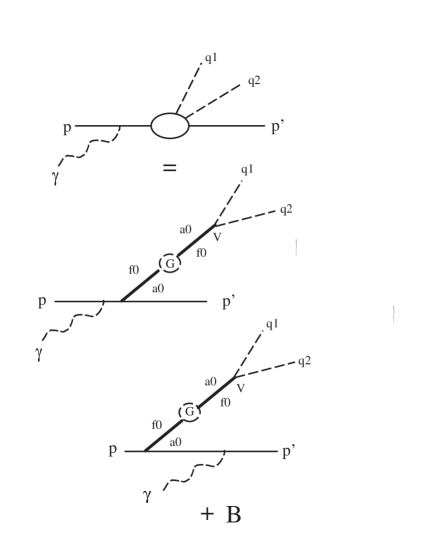
FIG. 1.: Feynman diagrams describing the doorway production of the reaction $\gamma p\to p^{\prime}m\bar{m}$. The total amplitude is a sum of these $f_{0}/a_{0}$ contributions plus the background $B,$ which is described in Fig. 2. The solid line with the blob $G$ insertion denotes the complete $f_{0}/a_{0}$ propagator (see Eq. 39) with $f_{0}\leftrightarrow a_{0}$ mixing. The decay mesons shown as dashed lines have momenta $q_{1}$ and $q_{2}.$

FIG. 2.: Feynman diagrams describing the possible background contributions $B$ for the the reaction $\gamma p\to p^{\prime}m\bar{m}.$ Dark solid lines stand for the contribution of resonances other than $f_{0}/a_{0}.$

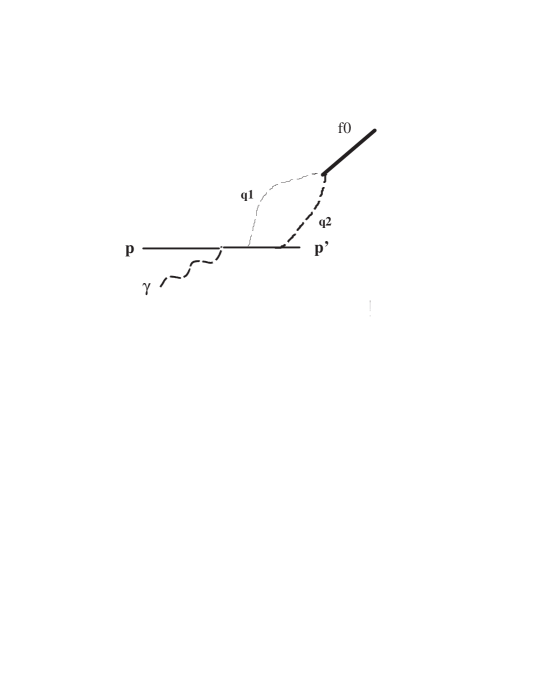
FIG. 3.: Production of $f_{0}$ via the pion loop as discussed in the text.

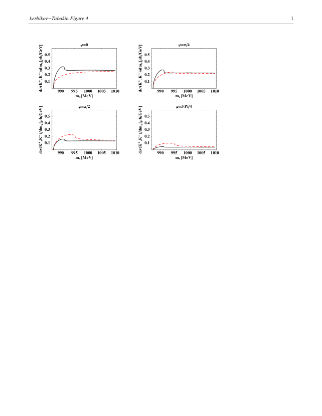
FIG. 4.: The invariant mass distribution $d\sigma(K^{+}K^{-})/dm_{x}$ in microbarns/GeV is plotted versus the invariant mass of the $K^{+}K^{-}$ pair resulting from scalar meson photoproduction. The dashed curve includes the $f_{0}\leftrightarrow a_{0}$ transitions caused by isospin breaking, whereas the solid curve is for case B for which the charged and neutral kaon masses are set equal to their average and the isospin effect is thus turned off. The dependence on the phase of the ratio $\zeta=|\zeta|\exp{i\phi}\equiv V_{K^{+}K^{-}a}/V_{K^{+}K^{-}f}$ is also shown, including the associated phase on the decay amplitudes $V_{K^{+}K^{-}a}$ and $V_{K^{+}K^{-}f}.$

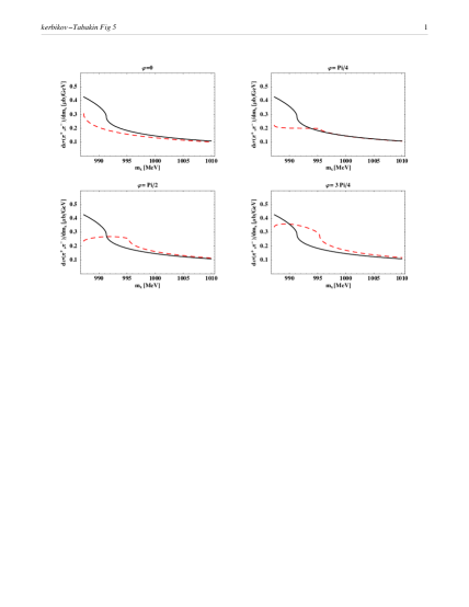
FIG. 5.: The invariant mass distribution $d\sigma(\pi^{+}\pi^{-})/dm_{x}$ in microbarns/GeV is plotted versus the invariant mass of the $\pi^{+}\pi^{-}$ pair resulting from scalar meson photoproduction. The dashed curve includes the $f_{0}\leftrightarrow a_{0}$ transitions caused by isospin breaking, whereas the solid curve is for set B for which the charged and neutral kaon masses are set equal to their average and the isospin effect is thus turned off. The dependence on the phase of the ratio $\zeta=|\zeta|\exp{i\phi}\equiv V_{K^{+}K^{-}a}/V_{K^{+}K^{-}f}$ is also shown. Here $V_{\pi^{+}\pi^{-}f}$ is taken as real. The same value of $R_{1}$ is used as in the kaon pair case.

- [1] Research supported in part by the U. S. National Science Foundation.
- [2] P.Lebrun in Proceedings of Hadron’97 Fermilab–Conf–97/388-E, E 687
- [3] The RADPHI JLAB experiment E-94-016.
- [4] Chueng-Ryong Ji et al., Phys. Rev. C58 (1998) 1205.
- [5] E. Marco, E. Oset and H. Toki, Phys. Rev. C60 (1999)015202.
- [6] N.N. Achasov, V.V. Gubin, and E.P. Solodov, Phys. Rev. D55 (1997) 2672; N.N. Achasov and V.V. Gubin, Phys. Rev. D56 (1997) 4084; N.N. Achasov and V.V. Gubin, Phys. Rev. D57 (1997) 1987;
- [7] R. R. Akhmetshin et al. preprint Budker INP 99-51.
- [8] J. A. Gomez Tejedor and E.Oset, Nucl. Phys. A571 (1994) 667.
- [9] S.Weinberg, Physica A96 (1979) 327; J. F. Donoghue, E. Golowich, and B. R. Holstein, Dynamics of the Standard Model, Cambridge Univ. Press, 1991, p.p. 105-109.
- [10] N.N. Achasov, S.A. Devyanin, and G.N. Shestakov, Phys. Lett. B88 (1979) 367.
- [11] T. Barnes, Phys. Lett. B165 (1985) 434.
- [12] L.Stodolsky, Resonance Mixing, preprint SLAC-Pub-776 (1970).
- [13] G.F.Chew et al. Phys. Rev. 106 (1957) 1345.
- [14] J.D.Bjorken and S.D.Drell, Relativistic Quantum Mechanics, McGraw–Hill 1964.
- [15] S.M.Bilenky et al., Soviet Physics Uspekhi 7 (1965) 721.
- [16] L.Stodolsky, Phys.Rev. D1 (1970) 2683
- [17] I.Kobzarev, N.Nikolaev and L.Okun, Yad. Fiz. 10 (1969) 864.
- [18] N. V. Terent’ev, Intoduction to Elementary Particle physics (in Russian), ITEP,Moscow, 1998, p.p. 180-190.
- [19] S.V.Bashinsky, B.Kerbikov, Physics of Atomic Nuclei, 59 (1996) 1979.
- [20] M. H. Ross and G. L. Shaw, Ann. Phys. 13 (1961) 147; M. H. Ross and G. L. Shaw, Phys. Rev. 126 (1962) 806.
- [21] B. S. Zou and D. V. Bugg, Phys. Rev. D48 (1993) R3948.
- [22] R. L. Jaffe, Phys. Rev. D15 (1977) 267.