The high-precision, charge-dependent Bonn nucleon-nucleon potential (CD-Bonn)

Abstract

We present a charge-dependent nucleon-nucleon ($NN$) potential that fits the world proton-proton data below 350 MeV available in the year of 2000 with a $\chi^{2}$ per datum of 1.01 for 2932 data and the corresponding neutron-proton data with $\chi^{2}$/datum $=1.02$ for 3058 data. This reproduction of the $NN$ data is more accurate than by any phase-shift analysis and any other $NN$ potential. The charge-dependence of the present potential (that has been dubbed ‘CD-Bonn’) is based upon the predictions by the Bonn Full Model for charge-symmetry and charge-independence breaking in all partial waves with $J\leq 4$. The potential is represented in terms of the covariant Feynman amplitudes for one-boson exchange which are nonlocal. Therefore, the off-shell behavior of the CD-Bonn potential differs in a characteristic and well-founded way from commonly used local potentials and leads to larger binding energies in nuclear few- and many-body systems, where underbinding is a persistent problem.

Contents

toc

I Introduction

In the 1970’s and 80’s, a comprehensive fieldtheoretic meson-exchange model for the nucleon-nucleon ($NN$) interaction was developed at the University of Bonn. The final version, published in 1987, has become known as the Bonn Full Model [1]. For a pedagogical review see Ref. [2].

In the language of fieldtheoretic perturbation theory, the lowest order contributions to the $NN$ interaction generated by mesons are the one-boson exchange diagrams. Furthermore, there are many irreducible multi-meson exchanges. The diagrams of $2\pi$ exchange are most prominent since they provide the intermediate-range attraction of the nuclear force. However, once explicit diagrams of $2\pi$ exchange (with intermediate $\Delta$ isobars) are used in a model, then it is vital to also include the corresponding diagrams of $\pi\rho$ exchange. There are characteristic (partial) cancellations between the two groups of diagrams, which are crucial for a quantitative reproduction of the $NN$ data. Moreover, the Bonn model contains additional classes of irreducible $3\pi$ and $4\pi$ exchanges which are important conceptually rather than quantitatively, since they appear to indicate convergence of the diagrammatic expansion chosen by the Bonn group [1].

The development of the Bonn Full Model was necessary to test reliably the meson-exchange concept for nuclear forces and to assess systematically the range of its validity. Thus, the model represents a benchmark for any alternative attempt (based, e. g., on quark models, chiral perturbation theory, or other ideas) to explain the nuclear force.

Due to its comprehensive character, the Bonn model provides a sound basis for addressing many important issues. One of them is the charge dependence of nuclear forces. The charge-symmetry-breaking (CSB) of the $NN$ interaction due to nucleon mass splitting has been investigated in Ref. [3]. It turns out that considerable CSB is generated by the $2\pi$-exchange contribution to the $NN$ interaction and the $\pi\rho$ diagrams such that the CSB difference in the singlet scattering lengths can be fully explained from nucleon mass splitting. Also, noticeable CSB effects occur in $P$ and $D$ waves. Empirical evidence for CSB is seen in the the Nolen-Schiffer (NS) anomaly [4] regarding the energies of neighboring mirror nuclei. A recent study [5] has shown that the CSB in partial waves with $L>0$ as derived from the Bonn model is crucial for a quantitative explanation of the NS anomaly.

The charge-independence breaking (CIB) of the $NN$ interaction has also been investigated [6]. Pion mass splitting is the major cause, and it is well-known that the one-pion-exchange (OPE) explains about 50% of the CIB difference in the singlet scattering lengths. However, the $2\pi$-exchange model and the diagrams of three and four irreducible pion exchanges contribute additional CIB which can amount up to 50% of the OPE CIB-contribution, in $S$, $P$, and $D$ waves. This effect is not negligible.

Other important issues related to the nuclear force are relativistic effects, medium effects, and many-body forces to be expected in the nuclear many-body problem. The medium effects on the nuclear force when inserted into nuclear matter have been calculated thoroughly. A large repulsive contribution to these medium effects comes from intermediate $\Delta$ isobar states which also give rise to energy-dependence. On the other hand, isobars create many-body forces that are attractive. Thus, large cancellations between these two classes of many-body forces/effects occur and it has been shown that the net contribution is very small [7]. Relativistic effects, however, may play an important role in the nuclear many-body problem [2].

Multi-meson exchange diagrams are very involved. Moreover, contributions of this kind are, in general, energy dependent. This would make the $NN$ potenital—defined as the sum of irreducible diagrams—energy dependent. A $NN$ potential that depends on energy creates conceptual and practical problems when applied in nuclear many-body systems. For a large class of nuclear structure problems, these complications are without merit.

For these reasons, already early in the history of the meson theory of nuclear forces, the so-called one-boson-exchange (OBE) model was designed which—by definition—includes only single-meson exchanges (which can be represented in an energy-independent way). Usually, the model includes all mesons with masses below the nucleon mass, i. e., $\pi$, $\eta$, $\rho(770)$, and $\omega(782)$ [8]. In addition, the OBE model typically introduces a scalar, isoscalar boson—commonly denoted by $\sigma$ (or $\epsilon$). Based upon what we discussed above concerning multi-meson exchange contributions, it is clear now that this $\sigma$ must approximate more than just the $2\pi$ exchange. In particular, it has to simulate $2\pi+\pi\rho$ exchanges which are clearly not of purely scalar, isoscalar nature. Consequently, the $\sigma$ approximation is poor (as demonstrated in Fig. 11 of Ref. [1]). One way to make up for this deficiency is to readjust the parameters of the $\sigma$ boson in each partial wave. Moreover, the $2\pi+\pi\rho$ exchanges create—in terms of ranges—a very broad contribution that cannot be reproduced well by a single boson-mass; two masses will do better. The fact that we are dealing here with a very broad mass distribution is supported by an entry in the Particle Data Tables [8] which lists a $\sigma$ (or $f_{0}$) with a mass between 400 and 1200 MeV.

Based upon the philosophy just outlined, we have constructed a $NN$ potential that is energy-independent and defined in the framework of the usual (nonrelativistic) Lippmann-Schwinger equation. Thus, it can be applied in the same way as any other conventional $NN$ potential. The crucial point, however, is that it reproduces important predictions by the Bonn Full Model, while avoiding the problems that the Bonn Full Model creates in applications. The charge-dependence (CD) predicted by the Bonn Full Model is reproduced accurately by the new potential, which is why we have dubbed it the CD-Bonn potential. The off-shell behavior of CD-Bonn is based upon the relativistic Feynman amplitudes for meson-exchange. Therefore, the CD-Bonn potential differs off-shell from conventional $NN$ potentials—a fact that has attractive consequences in nuclear structure applications.

An earlier version of the CD-Bonn potential—which, however, did not contain all the charge-dependence—was published in Ref. [9] where the off-shell aspects are discussed in great detail.

In Sec. II, we present the potential model. Charge dependence is discussed in Sec. III. The results for $NN$ scattering and the deuteron are presented in Sec. IV and V, respectively. Conclusions are given in Sec. VI. The paper has four appendices which contain mathematical and other details.

II The model

As discussed in the Introduction, the CD-Bonn potential is based upon meson exchange. We include all mesons with masses below the nucleon mass, i. e., $\pi$, $\eta$, $\rho(770)$, and $\omega(782)$. Besides this, we introduce two scalar-isoscalar $\sigma$ bosons.

For the $\eta$ (with a mass of 547.3 MeV), we assume a vanishing coupling to the nucleon, which implies that—de facto—we drop the $\eta$. This assumption is supported by semi-empirical evidence from various sources. Analyzing $NN$ scattering data in terms of forward dispersion relations, Grein and Kroll [10] determined the $\eta NN$ coupling constant to be consistent with zero. Tiator and coworkers [11] extracted the $\eta$ coupling from $\eta$ photoproduction data and found $g_{\eta}^{2}/4\pi=0.4$. Such a small coupling constant generates a negligible contribution in the $NN$ system. In the development of the Bonn Full Model for the $NN$ interaction [1], it was noticed that a good fit of the $NN$ data favors a vanishing $\eta$ contribution.

In Table I, we list the hadrons involved in our model together with their masses and coupling parameters. For the $\pi NN$ coupling constant, we choose the ‘small’ value $g_{\pi}^{2}/4\pi=13.6$—consistent with recent determinations by the Nijmegen [12, 13] and VPI group [14, 15, 16]. It is appropriate to mention that the precise value of the $\pi NN$ coupling constant is an unsettled issue at this time, and we refer the interested reader to Refs. [17, 18] for a critical discussion and review of the topic. For the vector mesons $\rho$ and $\omega$, for which precise empirical determinations of the coupling constants are difficult (if not impossible), we use the values from the Bonn Full Model [1].

We start from the following Lagrangians that describe the coupling of the mesons of interest to nucleons:

$${\cal L}_{\pi^{0}NN} = -g_{\pi^{0}}\bar{\psi}i\gamma^{5}\tau_{3}\psi\varphi^{(\pi^{0})}$$ (1)

$${\cal L}_{\pi^{\pm}NN} = -\sqrt{2}g_{\pi^{\pm}}\bar{\psi}i\gamma^{5}\tau_{\pm}\psi\varphi^{(\pi^{\pm})}$$ (2)

$${\cal L}_{\sigma NN} = -g_{\sigma}\bar{\psi}\psi\varphi^{(\sigma)}$$ (3)

$${\cal L}_{\omega NN} = -g_{\omega}\bar{\psi}\gamma^{\mu}\psi\varphi^{(\omega)}_{\mu}$$ (4)

$${\cal L}_{\rho NN} = -g_{\rho}\bar{\psi}\gamma^{\mu}\mbox{\boldmath$\tau$}\psi\cdot\mbox{\boldmath$\varphi$}^{(\rho)}_{\mu}-\frac{f_{\rho}}{4M_{p}}\bar{\psi}\sigma^{\mu\nu}\mbox{\boldmath$\tau$}\psi\cdot(\partial_{\mu}\mbox{\boldmath$\varphi$}^{(\rho)}_{\nu}-\partial_{\nu}\mbox{\boldmath$\varphi$}^{(\rho)}_{\mu})$$ (5)

where $\psi$ denotes nucleon fields, $\varphi$ meson fields, and $\tau_{3,\pm}$ are standard definitions of Pauli matrices and combinations thereof for isospin $\frac{1}{2}$ [19]. $M_{p}$ is the proton mass which is used as scaling mass in the $\rho NN$ Lagrangian to make $f_{\rho}$ dimensionless. To avoid the creation of unmotivated charge dependence, the scaling mass $M_{p}$ is used in the $\rho NN$ vertex no matter what nucleons are involved.

In the c. m. system of the two interacting nucleons, the OBE Feynman amplitude generated by meson $\alpha$ is,

$$-i\bar{V}_{\alpha}(q^{\prime},q)=\frac{\bar{u}_{1}({\bf q^{\prime}})\Gamma_{1}^{(\alpha)}u_{1}({\bf q})P_{\alpha}\bar{u}_{2}(-{\bf q^{\prime}})\Gamma_{2}^{(\alpha)}u_{2}(-{\bf q})}{(q^{\prime}-q)^{2}-m_{\alpha}^{2}}\;,$$ (6)

where $\Gamma_{i}^{(\alpha)}$ ($i=1,2$) are vertices derived from the above Lagrangians, $u_{i}$ Dirac spinors representing the interacting nucleons, and $q$ and $q^{\prime}$ their relative four-momenta in the initial and final states, respectively; $P_{\alpha}$ divided by the denominator is the appropriate meson propagator.

The one-boson-exchange potential is defined by ($i$ times) the sum over the OBE Feynman amplitudes of the mesons included in the model (Fig. 1); i. e.,

$$V({\bf q^{\prime}},{\bf q})=\sqrt{\frac{M}{E^{\prime}}}\sqrt{\frac{M}{E}}\sum_{\alpha=\pi^{0},\pi^{\pm},\rho,\omega,\sigma_{1},\sigma_{2}}\bar{V}_{\alpha}({\bf q^{\prime}},{\bf q}){\cal F}_{\alpha}^{2}({\bf q^{\prime}},{\bf q};\Lambda_{\alpha})\;.$$ (7)

As customary, we include form factors, ${\cal F}_{\alpha}({\bf q^{\prime}},{\bf q};\Lambda_{\alpha})$, applied to the meson-nucleon vertices, and a square-root factor $M/\sqrt{E^{\prime}E}$ (with $E=\sqrt{M^{2}+{\bf q}^{2}}$, $E^{\prime}=\sqrt{M^{2}+{\bf q^{\prime}}^{2}}$, and $M$ the nucleon mass). The form factors [see Appendix B, Eq. (B27), for details] regularize the amplitudes for large momenta (short distances) and account for the extended structure of nucleons in a phenomenological way. The square root factors make it possible to cast the unitarizing, relativistic, three-dimensional Blankenbecler-Sugar (BbS) equation [20] for the scattering amplitude [a reduced version of the four-dimensional Bethe-Salpeter (BS) equation [21]] into the following form (see Appendix A for a proper derivation):

$${T}({\bf q^{\prime}},{\bf q})={V}({\bf q^{\prime}},{\bf q})+\int d^{3}k\>{V}({\bf q^{\prime}},{\bf k})\>\frac{M}{{\bf q}^{2}-{\bf k}^{2}+i\epsilon}\>{T}({\bf k},{\bf q})$$ (8)

Notice that this is the familiar (non-relativistic) Lippmann-Schwinger equation. Thus, Eq. (7) defines a relativistic potential which can be consistently applied in conventional, non-relativistic nuclear structure, in the usual way.

The Feynman amplitudes, Eq. (6), are in general nonlocal expressions; i. e., Fourier transform into configuration space will yield functions of $r$ and $r^{\prime}$, the relative distances between the two in- and out-going nucleons, respectively. The square root factors in Eq. (7) create additional non-locality.

While for heavy vector-meson exchange (corresponding to short distances) non-locality appears quite plausible, we have to stress here that even the one-pion-exchange (OPE) Feynman amplitude is non-local. This fact is often overlooked. It is important because the pion creates the dominant part of the tensor force which plays a crucial role in nuclear structure.

Applying the $\pi NN$ Lagrangian Eq. (1) to the amplitude Eq. (6) yields the one-pion-exchange (OPE) potential (suppressing charge-dependence and isospin factors for the moment)

$$\bar{V}_{\pi}({\bf q^{\prime}},{\bf q}) = -\frac{g^{2}_{\pi}}{4M^{2}}\frac{(E^{\prime}+M)(E+M)}{({\bf q^{\prime}}-{\bf q})^{2}+m_{\pi}^{2}}\left(\frac{\mbox{\boldmath$\sigma_{1}\cdot$}{\bf q^{\prime}}}{E^{\prime}+M}-\frac{\mbox{\boldmath$\sigma_{1}\cdot$}{\bf q}}{E+M}\right)$$ (10)

$$\times\left(\frac{\mbox{\boldmath$\sigma_{2}\cdot$}{\bf q^{\prime}}}{E^{\prime}+M}-\frac{\mbox{\boldmath$\sigma_{2}\cdot$}{\bf q}}{E+M}\right)\,.$$

If we would now apply the approximation, $E^{\prime}\approx E\approx M$ (static approximation), then this simplifies to

$$V_{\pi}^{(loc)}({\bf k})=-\frac{g_{\pi}^{2}}{4M^{2}}\frac{{\mbox{\boldmath$(\sigma_{1}\cdot$}}{\bf k)}{\mbox{\boldmath$(\sigma_{2}\cdot$}}{\bf k)}}{{\bf k}^{2}+m_{\pi}^{2}}\;$$ (11)

with ${\bf k}={\bf q^{\prime}}-{\bf q}$. Fourier transform of this latter expression yields,

$$V_{\pi}^{(loc)}({\bf r}) = \frac{g^{2}_{\pi}}{12\pi}\left(\frac{m_{\pi}}{2M}\right)^{2}\left[\left(\frac{e^{-m_{\pi}r}}{r}-\frac{4\pi}{m_{\pi}^{2}}\delta^{(3)}({\bf r})\right)\mbox{\boldmath$\sigma_{1}\cdot\sigma_{2}$}\right.$$ (13)

$$+\left.\left(1+\frac{3}{m_{\pi}r}+\frac{3}{(m_{\pi}r)^{2}}\right)\frac{e^{-m_{\pi}r}}{r}\mbox{\boldmath$S_{12}$}\right]\>.$$

This is the local OPE potential that is used by most practitioners. However, the important point to notice here is that this local OPE is not the full, original OPE Feynman amplitude; it is an approximation.

The obvious question to raise at this point is: How much does the local approximation change the original result or, in other words, how drastic is the local approximation?

For this purpose, we show in Fig. 2 the half off-shell ${}^{3}S_{1}$–${}^{3}D_{1}$ potential that can be produced only by tensor forces. The on-shell momentum $q^{\prime}$ is held fixed at 265 MeV (equivalent to 150 MeV lab. energy), while the off-shell momentum $q$ runs from zero to 2000 MeV. The on-shell point ($q=265$ MeV) is marked by a solid dot. The solid curve is the relativistic OBE amplitude of $\pi+\rho$ exchange. Now, when the relativistic OPE amplitude, Eq. (10), is replaced by the static/local approximation, Eq. (11), the dashed curve is obtained. When this approximation is also used for the one-$\rho$ exchange, the dotted curve results. It is clearly seen that the static/local approximation does change the potential drastically off-shell: it makes the tensor force substantially stronger off-shell.

In summary, one characteristic point of the CD-Bonn potential is that it uses the Feynman amplitudes of meson exchange in its original form; local approximations are not applied. This has impact on the off-shell behavior of the potential, particularly, the off-shell tensor potential. It is well known that the off-shell behavior of an $NN$ potential is an important factor in microscopic nuclear structure calculations. Therefore, the predictions by the CD-Bonn potential for nuclear structure problems differ in a charcteristic way from the ones obtained with local $NN$ potentials. For more discussion of this issue, see Sec. VI and Refs. [9, 22].

III Charge dependence

By definition, charge independence is invariance under any rotation in isospin space. A violation of this symmetry is referred to as charge dependence or charge independence breaking (CIB). Charge symmetry is invariance under a rotation by 180⁰ about the $y$-axis in isospin space if the positive $z$-direction is associated with the positive charge. The violation of this symmetry is known as charge symmetry breaking (CSB). Obviously, CSB is a special case of charge dependence.

CIB of the strong $NN$ interaction means that, in the isospin $T=1$ state, the proton-proton ($T_{z}=+1$), neutron-proton ($T_{z}=0$), or neutron-neutron ($T_{z}=-1$) interactions are (slightly) different, after electromagnetic effects have been removed. CSB of the $NN$ interaction refers to a difference between proton-proton ($pp$) and neutron-neutron ($nn$) interactions, only. For recent reviews on these matters, see Refs. [23, 24].

CIB is seen most clearly in the ${}^{1}S_{0}$ $NN$ scattering lengths. The latest empirical values for the singlet scattering length $a$ and effective range $r$ are:

$$a^{N}_{pp}=-17.3\pm 0.4\mbox{ fm}\cite[cite]{[\@@bibref{Number}{MNS90}{}{}]},\hskip 22.76228pt r^{N}_{pp}=2.85\pm 0.04\mbox{ fm}\cite[cite]{[\@@bibref{Number}{MNS90}{}{}]};$$ (14)

$$a^{N}_{nn}=-18.9\pm 0.4\mbox{ fm}\cite[cite]{[\@@bibref{Number}{How98,Gon99}{}{}]},\hskip 4.55254pt r^{N}_{nn}=2.75\pm 0.11\mbox{ fm}\cite[cite]{[\@@bibref{Number}{MNS90}{}{}]};$$ (15)

$$a_{np}=-23.740\pm 0.020\mbox{ fm}\cite[cite]{[\@@bibref{Number}{KMS84}{}{}]}, r_{np}=2.77\pm 0.05\mbox{ fm}\cite[cite]{[\@@bibref{Number}{KMS84}{}{}]}.$$ (16)

The values given for $pp$ and $nn$ scattering refer to the nuclear part of the interaction as indicated by the superscript $N$; i. e., electromagnetic effects have been removed from the experimental values.

The above values imply that charge-symmetry is broken by the following amounts,

$$\Delta a_{CSB} \equiv a_{pp}^{N}-a_{nn}^{N}=1.6\pm 0.6\mbox{ fm},$$ (17)

$$\Delta r_{CSB} \equiv r_{pp}^{N}-r_{nn}^{N}=0.10\pm 0.12\mbox{ fm};$$ (18)

and, focusing on $pp$ and $np$, the following CIB is observed:

$$\Delta a_{CIB}\equiv a_{pp}^{N}-a_{np} = 6.44\pm 0.40\mbox{ fm},$$ (19)

$$\Delta r_{CIB}\equiv r_{pp}^{N}-r_{np} = 0.08\pm 0.06\mbox{ fm}.$$ (20)

In summary, the $NN$ singlet scattering lengths show a small amount of CSB and a clear signature of CIB.

The current understanding is that—on a fundamental level—the charge dependence of nuclear forces is due to a difference between the up and down quark masses and electromagnetic interactions among the quarks. As a consequence of this—on the hadronic level—major causes of CIB are mass differences between hadrons of the same isospin multiplet, meson mixing, and irreducible meson-photon exchanges.

A Charge symmetry breaking

The difference between the masses of neutron and proton represents the most basic cause for CSB of the nuclear force. Therefore, it is important to have a very thorough accounting of this effect.

The most trivial consequence of nucleon mass splitting is a difference in the kinetic energies: for the heavier neutrons, the kinetic energy is smaller than for protons. This raises the magnitude of the $nn$ scattering length by 0.26 fm as compare to $pp$. The nucleon mass difference also affects the OBE diagrams, Fig. 1, but only by a negligible amount. In summary, the two most obvious and trivial CSB effects explain only about 15% of the empirical $\Delta a_{CSB}$ (cf. Table II). Usual models for the nuclear force include only the two CSB effects just dicussed and, therefore, do not reproduce the empirical CSB.

However, in Ref. [3] it was found that the irreducible diagrams of two-boson exchange (TBE) create a much larger CSB effect than the OBE diagrams and, in fact, fully explain the empirical CSB splitting of the singlet scattering length. The major part of the CSB effect comes from diagrams of $2\pi$ exchange where those with $N\Delta$ intermediate states make the largest contribution. The CSB effect from irreducible diagrams that exchange a $\pi$ and $\rho$ meson were also included in the study. The $\pi\rho$ diagrams give rise to non-negligible CSB contributions that are typically smaller and of opposite sign as compared to the $2\pi$ effects. The net effect explains $\Delta a_{CSB}$ quantitatively.

The above-mentioned investigation [3] was based upon the Bonn Full Model [1]. This model uses the $\pi NN$ coupling constant $g^{2}_{\pi}/4\pi=14.4$ which is not current. For that reason we have revised the Bonn Full Model using $g^{2}_{\pi}/4\pi=13.6$ and then repeated the CSB calculations of Ref. [3]. The total $\Delta a_{CSB}$ predicted by the revised model is 1.508 fm (about 5% less than what was obtained in Ref. [3] with the original model), implying a TBE effect of 1.275 fm.

The only reliable empirical information about CSB of the $NN$ interaction is the scattering length difference in the ${}^{1}S_{0}$ state, Eq. (17). As discussed, the TBE model of Refs [1, 3] can explain this entirely from nucleon mass splitting. For this reason, we have confidence in the CSB predictions by this model. Therefore, we will use its predictions also for energies and states where no empirical information is available; namely, higher energies in the ${}^{1}S_{0}$ state and partial waves other than ${}^{1}S_{0}$.

Thus, using the revised Bonn Full Model, we have calculated the difference $nn$ phase shift minus $pp$ phase shift without electromagnetic interactions, $\delta_{nn}-\delta_{pp}$, that is caused by CSB of the strong nuclear force due to nucleon mass splitting. The total effect obtained is listed in the last colum (‘Total’) of Table III for energies up to 300 MeV and partial wave states in which these effects are non-negligible. In that table, we also list the very small effects from the OBE diagrams (Fig. 1) and the kinematical effects (column ‘Kinematics’) [30]. CSB phase shift differences are plotted in Fig. 3. It is clearly seen that in most states the TBE effect is the largest and, therefore, certainly not negligible as compared to the other CSB effects shown.

Because of the outstanding importance of the CSB effect from TBE, we include it in our model. By doing so, we go beyond what is usually done in charge-dependent $NN$ potentials. In most recent models, only the kinematical effects and the effect of nucleon mass splitting on the OBE diagrams are included. However, as discussed, this does not explain the CSB scattering length difference. Thus, some models leave CSB simply unexplained [31], while other models add a purely phenomenological term to the potential that fits $\Delta a_{CSB}$ [32].

Before finishing this subsection, a word is in place concerning other mechanisms that cause CSB of the nuclear force. Traditionally, it was believed that $\rho^{0}-\omega$ mixing explains essentially all CSB in the nuclear force [24]. However, recently some doubt has been cast on this paradigm. Some researchers [33, 34, 35, 36] found that $\rho^{0}-\omega$ exchange may have a substantial $q^{2}$ dependence such as to cause this contribution to nearly vanish in $NN$. Our finding that the empirically known CSB in the nuclear force can be explained solely from nucleon mass splitting (leaving essentially no room for additional CSB contributions from $\rho^{0}-\omega$ mixing or other sources) fits well into this scenario. On the other hand, Miller [23] and Coon and coworkers [37] have advanced counter-arguments that would restore the traditional role of $\rho$-$\omega$ exchange. The issue is unresolved. Good summaries of the controversial points of view can be found in Refs. [23, 38, 39]. We do not include $\rho-\omega$ mixing in our model.

Finally, for reasons of completeness, we mention that irreducible diagrams of $\pi$ and $\gamma$ exchange between two nucleons create a charge-dependent nuclear force. Recently, these contributions have been calculated to leading order in chiral perturbation theory [40]. It turns out that to this order the $\pi\gamma$ force is charge-symmetric (but does break charge independence).

B Charge independence breaking

The major cause of CIB in the $NN$ interaction is pion mass splitting. Based upon the Bonn Full Model for the $NN$ interaction, the CIB due to pion mass splitting has been calculated carefully and systematically in Ref. [6].

The largest CIB effect comes from the OPE diagram which accounts for about 50% of the empirical $\Delta a_{CIB}$, Eq. (19), (cf. Table IV).

In $pp$ scattering, the one-pion-exchange potential, $V^{OPE}$, is given by,

$$V^{OPE}(pp)=V_{\pi^{0}}\>,$$ (21)

while in $T=1$ $np$ scattering, we have,

$$V^{OPE}(np,T=1)=-V_{\pi^{0}}+2V_{\pi^{\pm}}\>.$$ (22)

If the pion masses were all the same, these would be identical potentials. However, due to the mass splitting, the $T=1$ $np$ potential is weaker as compared to the $pp$ one. This causes a difference between $T=1$ $pp$ and $np$ that is known as CIB. For completeness, we also give the $T=0$ $np$ OPE potential which is

$$V^{OPE}(np,T=0)=-V_{\pi^{0}}-2V_{\pi^{\pm}}\>.$$ (23)

Due to the small mass of the pion, OPE is also a sizable contribution in all partial waves with $L>0$; and due to the pion’s relatively large mass splitting (3.4%), OPE creates relatively large charge-dependent effects in all partial waves (cf. Tables V and VI and Fig. 4). Therefore, all modern phase shift analyses [14, 42] and all modern $NN$ potentials [31, 32, 9] include the CIB effect created by OPE.

However, pion mass splitting creates further CIB effects through the diagrams of $2\pi$ exchange and other two-boson exchange diagrams that involve pions. The evaluation of this CIB contribution is very involved, but it has been accomplished in Ref. [6]. The CIB effect from all the relevant two-boson exchanges (TBE) contributes about 1.3 fm to $\Delta a_{CIB}$. Concerning phase shift differences, it is noticable up to $D$ waves and can amount up to 50% of the OPE effect in some states (cf. Tables V and VI [43]).

Another source of CIB is irreducible $\pi\gamma$ exchange. Recently, these contributions have been evaluated in the framework of chiral perturbation theory by van Kolck et al. [40]. Based upon this work, we have calculated the impact of the $\pi\gamma$ diagrams on the ${}^{1}S_{0}$ scattering length and on $np$ phase shifts. (see column ‘$\pi\gamma$’ in Tables IV, V, and VI). In $L>0$ states, the size of this contribution is typically the same as the CIB effect from TBE.

In the ${}^{1}S_{0}$ state, the $\pi\gamma$ contribution increases the discrepancy between theory and experiment (cf. Table IV). As a matter of fact, about 25% of $\Delta a_{CIB}$ is not explained. For that reason, a quantitative fit of the empirical $\Delta a_{CIB}$ requires a small phenomenological contribution. The same is true for the difference between the empirical $np$ and $pp$ phase shifts in the ${}^{1}S_{0}$ state (cf. Table V).

For convenience, the major CIB effects on the strong $NN$ force are plotted in Fig. 4. In Fig. 5 the total CIB phase shift effect caused by the strong force is compared to the Coulomb effect on $pp$ phase shifts ($\delta^{C}$ denotes the phase shift in the presence of the Coulomb force, see Appendix A.3 for precise definitions of $\delta$ and $\delta^{C}$).

From the figures and tables it is evident that TBE and $\pi\gamma$ create sizable CIB effects in states with $L>0$. Therefore, we will include these two effects in our model. We note that conventional charge-dependent $NN$ models ignore these two contributions.

IV Nucleon-nucleon scattering

We construct three $NN$ interactions: a proton-proton ($pp$), a neutron-neutron ($nn$), and a neutron-proton ($np$) potential. The three potentials are not independent. They are all based upon the model described in Sec. II and the differences between them are determined by CSB and CIB as discussed in Sec. III. Thus, when one of the three potentials is fixed, then the $T=1$ parts of the other two potentials are also fixed due to CSB and CIB.

We start with the $pp$ potential since the $pp$ data are the most accurate ones. Data fitting is done in three steps. In the first step, the $pp$ potential is adjusted to reproduce closely the $pp$ phase shifts of the Nijmegen multi-energy $pp$ phase shift analysis [42]. This is to ensure that phase shifts are in the right ballpark. In the second step, the $\chi^{2}$ that results from applying the Nijmegen $pp$ error matrix [44] is minimized. The error matrix allows to calculate the $\chi^{2}$ in regard to the $pp$ data in an approximate way requirings little computer time. Finally, in the third and crucial step, the $pp$ potential parameters are fine-tuned by minimizing the exact $\chi^{2}$ that results from a direct comparison with all experimental $pp$ data. During these calculations, it was revealed that the Nijmegen $pp$ error matrix yields very accurate $\chi^{2}$ up to 75 MeV. Therefore, in this final step, we used the error matrix up to 75 MeV and direct $\chi^{2}$ calculations above this energy.

The $nn$ potential is constructed by starting from the $pp$ potential, leaving out the Coulomb force, changing the nucleon masses, and fine-tuning the parameters such that the CSB differences listed in Tables II and III are reproduced.

Concerning the $np$ potential, we need to distinguish between the $T=0$ and $T=1$ states. In $T=1$, we start from the $pp$ potential, leave out the Coulomb force, change the nucleon masses, and replace the $pp$ OPE potential by the one that applies to $np$. This produces a large part of CIB. The additional CIB due to TBE and $\pi\gamma$ discussed in Sec. III is incorporated by fine-tuning the parameters such that the total CIB phase shift differences as given in Table VI are reproduced. This fixes the $np$ potential in the $T=1$ states with $L>0$. The ${}^{1}S_{0}$ $np$ potential is adjusted such as to minimize the $\chi^{2}$ in regard to the $np$ data. The $np$ $T=0$ potential is fixed by going through the entire three-step procedure: fit of Nijmegen $T=0$ phase shifts, minimizing the approximate $\chi^{2}$ obtained from the Nijmegen error matrix, and finally minimizing the exact $\chi^{2}$ that results from a direct comparison with all experimental $np$ data.

The resulting phase shifts for $pp$, $nn$, and $np$ scattering in partial waves with $J\leq 4$ are given in Tables VII – X; $pp$ phase shifts are plotted in Fig. 6 and $np$ phase shifts are shown in Fig. 7. For $pp$ scattering, we show the phase shifts of the nuclear plus relativistic Coulomb interaction with respect to Coulomb wave functions; that is—in the notation of Ref. [46]—we use $V_{C}=\alpha^{\prime}/r$ for the Coulomb potential and calculate the phase shifts $\delta^{C}_{C+N}$ ($\equiv\delta^{C}$ in our notation). We note that, for the calculation of observables (e. g., to obtain the $\chi^{2}$ in regard to experimental data), we use electromagnetic phase shifts, as necessary, which we obtain by adding to the Coulomb phase shifts the effects from two-photon exchange, vacuum polarization, and magnetic moment interactions as calculated by the Nijmegen group [46, 47]. This is important for ${}^{1}S_{0}$ below 30 MeV and negligible otherwise. For $nn$ and $np$ scattering, we show the phase shifts of the nuclear interaction with respect to Riccati-Bessel functions. All details of our phase shift calculations are given in Appendix A.3

The low-energy scattering parameters are shown in Table XI. For $nn$ and $np$, the effective range expansion without any electromagnetic interaction is used. In the case of $pp$ scattering, the quantities $a_{pp}^{C}$ and $r_{pp}^{C}$ are obtained by using the effective range expansion appropriate in the presence of the Coulomb force (see Appendix A.4 for details). Note that the empirical values for $a_{pp}^{C}$ and $r_{pp}^{C}$ that we quote in Table XI were obtained by subtracting from the corresponding electromagnetic values the effects due to two-photon exchange and vacuum polarization. Thus, the comparison between theory and experiment conducted in Table XI is adequate.

For the comparison with the $NN$ data, we consider three databases: 1992 database, after-1992 data, and 1999 database. The 1992 database is identical to the one used by the Nijmegen group for their phase shift analysis [49, 42]. It consists of all $NN$ data below 350 MeV published between January 1955 and December 1992 that were not rejected in the Nijmegen data analysis (for details of the rejection criteria and a complete listing of the data references, see Refs. [46, 49, 42]). The 1992 database contains 1787 $pp$ data and 2514 $np$ data.

After 1992, there has been a fundamental breakthrough in the development of experimental methods for conducting hadron-hadron scattering experiments. In particular, the method of internal polarized gas targets applied in stored, cooled beams is now working perfectly in several hadron facilities, e. g., IUCF and COSY. Using this new technology, IUCF has produced a large number of $pp$ spin correlation parameters of very high precision. In Table XII, we list the new IUCF data together with other $pp$ data published between January 1993 and December 1999. Table XII lists all published after-1992 $pp$ data below 350 MeV except for one set, namely, 14 $pp$ differential cross sections at 45 deg (lab.) between 299.8 adn 406.8 keV by Dombrowski et al. [56]; according to the Nijmegen rejection criteria [46], this set is to be discarded. The total number of (accepted) after-1992 $pp$ data is 1145, which should be compared to the number of $pp$ data in the 1992 base, namely, 1787. Thus, the $pp$ database has increased by about 2/3 since 1992. The importance of the new $pp$ data is further enhanced by the fact that they are of much higher quality than the old ones.

Neutron-proton data published between January 1993 and December 1999 and included in our $\chi^{2}$ calculations are listed in Table XIII. There are 544 such data, which is a small number as compared to the 2514 $np$ data of the 1992 base. Note that Table XIII is not a list of all $np$ data published after 1992. Not listed are four measurements of $np$ differential cross sections [67, 68, 69, 70]. We have examined these data and found in each case that they produced an improbably high $\chi^{2}$ when compared to current phase shift analyses [42, 45]. Applying the Nijmegen rejection rule [46, 42], the data of all four experiments are to be discarded. We follow this rule here, because we use the Nijmegen database for the pre-1993 period. When we add data to this base, then consistency requires that we apply the same selection criteria used for assembling the older part of the base. However, we like to stress that we do understand that any discarding of published data (i. e., data that have passed the refereeing process) is a highly questionable procedure. The problem of the $np$ differential cross section data is an unresolved issue that deserves the full attention of all $NN$ practitioners. Some aspects of the problem were recently discussed in Ref. [71].

Finally, our 1999 database is the sum of the 1992 base and the after-1992 data and, thus, consists of the world $NN$ data below 350 MeV that were published before the year of 2000 (and not rejected).

The $\chi^{2}$/datum produced by the CD-Bonn potential in regard to the databases defined above are listed in Table XIV. For the purpose of comparison, we also give the corresponding $\chi^{2}$ values for the Nijmegen phase shift analysis [42] and the recent Argonne $V_{18}$ potential [32]. What stands out in Table XIV are the rather large values for the $\chi^{2}$/datum generated by the Nijmegen analysis and the Argonne potential for the the after-1992 $pp$ data, which are essentially the new IUCF data. This fact is a clear indication that these new data provide a very critical test/constraint for any $NN$ model. It further indicates that fitting the pre-1993 $pp$ data does not nessarily imply a good fit of those IUCF data. On the other hand, fitting the new IUCF data does imply a good fit of the pre-1993 data. The conclusion from these two facts is that the new IUCF data provide information that was not contained in the old database. Or, in other words, the pre-1993 data were insufficient and still left too much lattitude for pinning down $NN$ models. One thing in particular that we noticed is that the ${}^{3}P_{1}$ phase shifts above 100 MeV have to be lower than the values given in the Nijmegen analysis.

The bottom line is that, for the 1999 data base (which contains 5990 $pp$ and $np$ data), the CD-Bonn potential yields a $\chi^{2}$/datum of 1.02, while the Nijmegen analysis produces 1.04 and the Argonne potential 1.21. We have also compared other recent $NN$ potentials and $NN$ analyses to the 1999 database and found in all case a $\chi^{2}$/datum $\geq 1.05$.

Thus we can conclude that the CD-Bonn potential fits the world $NN$ data below 350 MeV available in the year of 2000 better than any phase shift analysis and any other $NN$ potential.

V The deuteron

The CD-Bonn potential has been fitted to the empirical value for the deuteron binding energy $B_{d}=2.224575$ MeV [72] using relativistic kinematics. Once this adjustment has been made, the other deuteron properties listed in in Table XV are predictions. For the asymptotic $D/S$ state ratio, we find $\eta=0.0256$—in accurate agreement with the empirical determination by Rodning and Knutson [74]. The deuteron matter radius is predicted to be $r_{d}=1.966$ fm which agrees well with the value extracted from recent hydrogen-deuterium isotope shift measurements, $r_{d}=1.971(6)$ fm [75]. Note that the deuteron effective range $\rho_{d}\equiv\rho(-B_{d},-B_{d})$ and the asymptotic $S$ state $A_{S}$ are not directly observable quantities. Thus, ‘empirical’ values for $\rho_{d}$ and $A_{S}$ quoted in the literature are model dependent. Therefore, the perfect agreement between our predictions and the empirical values for $\rho_{d}$ and $A_{S}$ is of no fundamental significance. It only means that all models (including our own) are consistent with each other.

More interesting is our prediction for the deuteron quadrupole moment $Q_{d}=0.270$ fm² which is below the empirical value of 0.2859(3) fm² [76, 73]. Our calculation does not include relativistic and meson current corrections which according to Henning [77] contribute typically about 0.010 fm² for the Bonn OBE potentials. This would raise our theoretical value to $Q_{d}\approx 0.280$ fm², still 0.006 fm² below experiment. All recent $NN$ potentials that use the ‘small’ $\pi NN$ coupling constant $g^{2}_{\pi}/4\pi=13.6$ underpredict $Q_{d}$ by about the same amount. In Refs. [78, 17] it was shown that $Q_{d}$ depends sensitively on $g_{\pi}$ and that a value $g^{2}_{\pi}/4\pi\geq 14.0$ would solve the problem. However, a larger $g_{\pi}$ is inconsistent with the low-energy $pp$ $A_{y}$ data (see Ref. [17] for a detailed discussion of this issue). Thus, the accurate explanation of the deuteron quadrupole moment is an unresolved problem at this time.

In Table XV, we also give the deuteron $D$-state probability $P_{D}$. This quantity is not an observable, but it is of great theoretical interest. CD-Bonn predicts $P_{D}=4.85$% while local potentials typically predict $P_{D}\approx 5.7$ %, which is clearly reflected in the deuteron $D$-waves, Figs. 8 and 9. The smaller $P_{D}$ value of CD-Bonn can be traced to the non-localities contained in the tensor force as discussed in Sec. II and demonstrated in Fig. 2. The CD-Bonn and the Nijmegen-I [31] potentials have nonlocal central forces which explains the soft behavior of their deuteron $S$-waves at short distances that is particularly apparent in the plot of Fig. 9. Numerical values of our deuteron waves and a convenient parametrization are given in Appendix D which also contains an account of how to conduct deuteron calculations in momentum space.

VI Conclusions

We have constructed charge-dependent $NN$ potentials, that fit the world proton-proton data below 350 MeV (2932 data) with a $\chi^{2}$/datum of 1.01 and the corresponding neutron-proton data (3058 data) with $\chi^{2}$/datum $=1.02$. This reproduction of the $NN$ data is more accurate than by any other known $NN$ potential or phase-shift analysis. A particular challenge are the $pp$ spin correlation parameters that were recently measured at the IUCF Cooler Ring with very high precision (1126 data below 350 MeV). Our $pp$ potential reproduces these data with $\chi^{2}$/datum $=1.03$, while the high-quality Nijmegen analysis [42] and the Argonne $V_{18}$ potential [32] produce $\chi^{2}$/datum of 1.24 and 1.74, respectively, for these data.

The charge-dependence of the present potential (that has been dubbed ‘CD-Bonn’) is based upon the predictions by the Bonn Full Model for charge-symmetry and charge-independence breaking in all partial waves with $J\leq 4$. Thus, our model includes considerably more charge-dependence than other recently developed charge-dependent potentials [31, 32]. For example, the Nijmegen potentials [31] include essentially only charge-dependence due to OPE which produces CIB, but no CSB. Thus, the Nijmegen group does not offer any genuine neutron-neutron potentials. To have distinct $pp$ and $nn$ potentials is important for addressing several interesting issues in nuclear physics, like the ³H-³He binding energy difference for which the CD-Bonn potential predicts 60 keV in agreement with empirical estimates. Another issue is the Nolen-Schiffer anomaly [4]. Some potentials that include CSB focus on the ${}^{1}S_{0}$ state only, since this is where the most reliable empirical information is. However, this is not good enough. In Ref. [5] it has been shown that CSB in states with $J>0$ is crucial for the explanation of the Nolen-Schiffer anomaly.

The CD-Bonn potential is represented in terms of the covariant Feynman amplitudes for one-boson exchange which are nonlocal. Therefore, the off-shell behavior of the CD-Bonn potential differs in a characteristic and well-founded way from the one of commonly used local potentials.

The simplest system in which off-shell differences between $NN$ potentials can be investigated is the deuteron (see Ref. [79] for a thorough study of this issue). Our plots of the deuteron wave functions, Figs. 8 and 9, make this point very clear. Empirical tests of deuteron wave functions can be conducted via the structure functions $A(Q^{2})$, $B(Q^{2})$, and the tensor polarization in elastic electron-deuteron scattering $T_{20}(Q^{2})$ or, alternatively, via the three deuteron form factors $G_{C}(Q^{2})$, $G_{Q}(Q^{2})$, and $G_{M}(Q^{2})$, for which the deuteron wave functions are crucial input. Using the deuteron wave functions derived from the Bonn model, Arenhövel and coworkers [80] find a good agreement between theory and experiment for $A(Q^{2})$, $B(Q^{2})$, and $T_{20}(Q^{2})$ up to $Q^{2}=30$ fm^-2. Very recently, the tensor polarization $T_{20}(Q^{2})$ has been measured up to $Q^{2}=45$ fm^-2 at the Jefferson Laboratory [81]. The best reproduction of these new high-precision data is provided by two calculations that are based upon the Bonn deuteron wave functions [82, 83].

Another way in which the off-shell behavior of our potential shows up is by yielding larger binding energies in microscopic calculations of nuclear few- and many-body systems [84], where underbinding is a persistent problem. To demonstrate this, we have computed the binding energy of the triton in a 34-channel, charge-dependent Faddeev calculation. The prediction by the CD-Bonn potential is 8.00 MeV. Local potentials typically predict 7.62 MeV [85, 86] and the experimental value is 8.48 MeV. Thus, the nonlocality of the CD-Bonn potential explains almost 50% of the gap that persists between the predictions by local potentials and experiment. Similar results are obtained for the $\alpha$ particle [86, 87]. Concerning the small difference that is left between the CD-Bonn predictions and experiment, two comments are in place. First, besides the relativistic, nonlocal effects that can be absorbed into the two-body potential concept, there are further relativistic corrections that come from a relativistic treatment of the three-body system. This increases the triton binding energy by 0.2–0.3 MeV [88, 89, 90, 9]. Second, notice that the present nonlocal potential includes only the nonlocalities that come from meson-exchange. However, the composite structure (quark substructure) of hadrons should provide additional nonlocalities [91] which may be even larger. It is a challenging topic for future research to derive these additional nonlocalities, and test their impact on nuclear structure predictions.

The trend of the nonlocal Bonn potential to increase binding energies has also a very favorable impact on predictions for nuclear matter [7, 22] and the structure of finite nuclei [92, 93, 94].

Due to the very accurate fit of even the latest high-precision $NN$ data; due to the comprehensive and sophisticated charge-dependence incorporated in the model; and due to the well-founded off-shell behavior, the CD-Bonn potential [95] represents a promising starting point for exact few-body calculations and microscopic nuclear many-body theory.

A Two-nucleon scattering in momentum space

1 Scattering equation

Two-nucleon scattering is described covariantly by the Bethe-Salpeter (BS) equation [21] which reads in operator notation

$${\cal T=V+VGT}$$ (A1)

with ${\cal T}$ the invariant amplitude for the two-nucleon scattering process, ${\cal V}$ the sum of all connected two-particle irreducible diagrams, and ${\cal G}$ the relativistic two-nucleon propagator. Since this four-dimensional integral equation is very difficult to solve, so-called three-dimensional reductions have been proposed, which are more amenable to numerical solution. Furthermore, it has been shown by Gross [96] that the full BS equation in ladder approximation (that is, the kernel ${\cal V}$ is restricted to the exchange of single particles as, e. g., in the OBE model) does not have the correct one-body limit (i. e., when one of the particles becomes very massive) while a large family of three-dimensional quasi-potential equations does. These approximations to the BS equation are also covariant and satisfy relativistic elastic unitarity. Three-dimensional reductions are typically derived by replacing Eq. (A1) with two coupled equations [97]:

$${\cal T=W+W}g{\cal T}$$ (A2)

and

$${\cal W=V+V(G}-g){\cal W}$$ (A3)

where $g$ is a covariant three-dimensional propagator with the same elastic unitarity cut as ${\cal G}$ in the physical region. In general, the second term on the r.h.s. of Eq. (A3) is dropped to obtain a true simplification of the problem.

More explicitly, the BS equation for an arbitrary frame reads [19]

$${\cal T}(q^{\prime};q|P)={\cal V}(q^{\prime};q|P)+\int d^{4}k\>{\cal V}(q^{\prime};k|P)\>{\cal G}(k|P)\>{\cal T}(k;q|P)$$ (A4)

with

$${\cal G}(k|P) = \frac{i}{2\pi}\frac{1}{(\frac{1}{2}\not\!P+\not\!k-M+i\epsilon)^{(1)}}\frac{1}{(\frac{1}{2}\not\!P-\not\!k-M+i\epsilon)^{(2)}}$$ (A5)

$$= \frac{i}{2\pi}\left[\frac{\frac{1}{2}\not\!P+\not\!k+M}{(\frac{1}{2}P+k)^{2}-M^{2}+i\epsilon}\right]^{(1)}\left[\frac{\frac{1}{2}\not\!P-\not\!k+M}{(\frac{1}{2}P-k)^{2}-M^{2}+i\epsilon}\right]^{(2)}$$ (A6)

where $q$, $k$, and $q^{\prime}$ are the initial, intermediate, and final relative four-momenta, respectively, and $P=(P_{0},{\bf P})$ is the total four-momentum. For example, in the initial state we have: $q=\frac{1}{2}(p_{1}-p_{2}),P=p_{1}+p_{2},\mbox{ and }p_{1/2}=\frac{1}{2}P\pm q$ with $p_{1}$ and $p_{2}$ the individual four-momenta of particle 1 and 2. In the center-of-mass (c.m.) frame, we will have $P=(\sqrt{s},{\bf 0})$ with $\sqrt{s}$ the total energy. For all four-momenta, our notation is $k=(k_{0},{\bf k})$; $\not\!\!k\equiv\gamma^{\mu}k_{\mu}$. $M$ denotes the nucleon mass. The superscripts in Eq. (A6) refer to particle (1) and (2). At this stage, ${\cal T,V,\mbox{ and }G}$ are operators in spinor space, i. e. they are $16\times 16$ matrices which, when sandwiched between Dirac spinors, yield the corresponding matrix elements.

It is common to the derivation of all three-dimensional reductions that the time component of the relative momentum is fixed in some covariant way, so that it no longer appears as an independent variable in the propagator.

Following Blankenbecler and Sugar (BbS) [20], one possible choice for $g$ is (stated in manifestly covariant form for an arbitrary frame)

$$g_{BbS}(k,s) = -\int_{4M^{2}}^{\infty}\frac{ds^{\prime}}{s^{\prime}-s-i\epsilon}\>\delta^{(+)}[\begin{array}[]{c}(\frac{1}{2}P^{\prime}+k)^{2}-M^{2}\end{array}]$$ (A13)

$$\times\delta^{(+)}[\begin{array}[]{c}(\frac{1}{2}P^{\prime}-k)^{2}-M^{2}\end{array}]$$

$$\times[\begin{array}[]{c}\frac{1}{2}\not\!P^{\prime}+\not\!k+M\end{array}]^{(1)}[\begin{array}[]{c}\frac{1}{2}\not\!P^{\prime}-\not\!k+M\end{array}]^{(2)}$$

with $\delta^{(+)}$ indicating that only the positive energy root of the argument of the $\delta$-function is to be included; $P^{2}=s$ and $P^{\prime}\equiv\frac{\sqrt{s^{\prime}}}{\sqrt{s}}P$. By construction, the propagator $g_{BbS}$ has the same imaginary part as ${\cal G}$ and, therefore, preserves the unitarity relation satisfied by ${\cal T}$. In the c.m. frame, integration yields

$$g_{BbS}(k,s)=\delta(k_{0})\>\bar{g}_{BbS}({\bf k},s)$$ (A14)

with

$$\bar{g}_{BbS}({\bf k},s)=\frac{M^{2}}{E_{k}}\>\frac{\Lambda_{+}^{(1)}({\bf k})\>\Lambda_{+}^{(2)}({\bf-k})}{\frac{1}{4}s-E^{2}_{k}+i\epsilon}$$ (A15)

where

$$\Lambda^{(i)}_{+}({\bf k}) = \left(\frac{\gamma^{0}E_{k}-{\mathchoice{{\hbox{\boldmath$\displaystyle\gamma$}}}{{\hbox{\boldmath$\textstyle\gamma$}}}{{\hbox{\boldmath$\scriptstyle\gamma$}}}{{\hbox{\boldmath$\scriptscriptstyle\gamma$}}}}\cdot{\bf k}+M}{2M}\right)^{(i)}$$ (A16)

$$= \sum_{\lambda_{i}}|u({\bf k},\lambda_{i})\rangle\langle\bar{u}({\bf k},\lambda_{i})|$$ (A17)

represents the positive-energy projection operator for nucleon $i$ ($i$ = 1 or 2) with $u({\bf k})$ a positive-energy Dirac spinor of momentum ${\bf k}$; $\bar{u}\equiv u^{\dagger}\gamma^{0}$. $\lambda_{i}$ denotes the helicity of the respective nucleon, and $E_{k}\equiv\sqrt{M^{2}+{\bf k}^{2}}$ with $M$ the nucleon mass. The projection operators imply that virtual anti-nucleon contributions are suppressed.

Using the approximation ${\cal W}\approx{\cal V}$ [cf. Eq. (A3)], we obtain the explicit form of Eq. (A2) by simply replacing ${\cal G}$ by $g_{BbS}$ in Eq. (A4). This yields in the c.m. frame

$${\cal T}(0,{\bf q^{\prime}};0,{\bf q}|\sqrt{s})={\cal V}(0,{\bf q^{\prime}};0,{\bf q})+\int d^{3}k\>{\cal V}(0,{\bf q^{\prime}};0,{\bf k})\>\bar{g}_{BbS}({\bf k},s)\>{\cal T}(0,{\bf k};0,{\bf q}|\sqrt{s}).$$ (A18)

Note that four-momentum is conserved at each vertex, and that in the initial state the nucleons are on their mass-shell, therefore $q=(0,{\bf q})$. The total c.m. energy is

$$\sqrt{s}=2E_{q}=2\sqrt{M^{2}+{\bf q}^{2}}.$$ (A19)

With this we obtain, simplifying our notation,

$${\cal T}({\bf q^{\prime}},{\bf q})={\cal V}({\bf q^{\prime}},{\bf q})+\int d^{3}k\>{\cal V}({\bf q^{\prime}},{\bf k})\>\frac{M^{2}}{E_{k}}\>\frac{\Lambda_{+}^{(1)}({\bf k})\>\Lambda_{+}^{(2)}({\bf-k})}{{\bf q}^{2}-{\bf k}^{2}+i\epsilon}\>{\cal T}({\bf k},{\bf q}).$$ (A20)

Taking matrix elements between positive-energy spinors yields an equation for the invariant scattering amplitude

$$\bar{T}({\bf q^{\prime}},{\bf q})=\bar{V}({\bf q^{\prime}},{\bf q})+\int d^{3}k\>\bar{V}({\bf q^{\prime}},{\bf k})\>\frac{M^{2}}{E_{k}}\>\frac{1}{{\bf q}^{2}-{\bf k}^{2}+i\epsilon}\>\bar{T}({\bf k},{\bf q}),$$ (A21)

where helicity and isospin indices are suppressed.
Defining

$${T}({\bf q^{\prime}},{\bf q})=\sqrt{\frac{M}{E_{q^{\prime}}}}\>\bar{T}({\bf q^{\prime}},{\bf q})\>\sqrt{\frac{M}{E_{q}}}$$ (A22)

and

$${V}({\bf q^{\prime}},{\bf q})=\sqrt{\frac{M}{E_{q^{\prime}}}}\>\bar{V}({\bf q^{\prime}},{\bf q})\>\sqrt{\frac{M}{E_{q}}},$$ (A23)

which has become known as “minimal relativity” [98], we can rewrite Eq. (A21) as

$${T}({\bf q^{\prime}},{\bf q})={V}({\bf q^{\prime}},{\bf q})+\int d^{3}k\>{V}({\bf q^{\prime}},{\bf k})\>\frac{M}{{\bf q}^{2}-{\bf k}^{2}+i\epsilon}\>{T}({\bf k},{\bf q})$$ (A24)

which has the form of the familiar Lippmann-Schwinger equation. The quantity $T$ has the usual (nonrelativistic) relation to phase shifts and $NN$ observables. Thus, the $NN$ potential $V$ defined in Eq. (A23) and used in the above Lippmann-Schwinger equation can be applied in the deuteron and in conventional nuclear structure physics in the same way as any other (nonrelativistic) potential. This is the great virtue of the (relativistic) BbS equation.

2 R-matrix and partial wave decomposition

In solving the scattering equation, it is more convenient to deal with real quantities. We shall therefore introduce the real $R$-matrix (better known as ‘$K$-matrix’) defined by

$$T=R-i\pi R\delta(E-H_{0})T$$ (A25)

The equation for the real ${R}$-matrix corresponding to the complex ${T}$-matrix of Eq. (A24) is

$${R}({\bf q^{\prime}},{\bf q})={V}({\bf q^{\prime}},{\bf q})+{\cal P}\int d^{3}k\>{V}({\bf q^{\prime}},{\bf k})\>\frac{M}{{\bf q}^{2}-{\bf k}^{2}}\>{R}({\bf k},{\bf q})$$ (A26)

where ${\cal P}$ denotes the principal value.

Now, we need to also include the spin of the nucleons. Relativistic scattering of particles with spin is treated most conveniently in the helicity formalism [99]. Therefore, we will use a helicity state basis in our further formal developments. Our presentation will be relatively brief; a more detailed derivation is given in Appendix C of Ref. [1] which is based upon Refs. [99, 100].

The helicity $\lambda_{i}$ of particle $i$ (with $i=1$ or 2) is the eigenvalue of the helicity operator $\frac{1}{2}\mathchoice{{\hbox{\boldmath$\displaystyle\sigma$}}}{{\hbox{\boldmath$\textstyle\sigma$}}}{{\hbox{\boldmath$\scriptstyle\sigma$}}}{{\hbox{\boldmath$\scriptscriptstyle\sigma$}}}_{i}\cdot{\bf p}_{i}/|{\bf p}_{i}|$ which is $\pm\frac{1}{2}$.

Using helicity states, the ${R}$-matrix equation reads, after partial wave decomposition,

$$\langle\lambda_{1}^{\prime}\lambda_{2}^{\prime}|{R}^{J}(q^{\prime},q)|\lambda_{1}\lambda_{2}\rangle = \langle\lambda_{1}^{\prime}\lambda_{2}^{\prime}|{V}^{J}(q^{\prime},q)|\lambda_{1}\lambda_{2}\rangle$$ (A29)

$$\mbox{}+\sum_{h_{1},h_{2}}{\cal P}\int^{\infty}_{0}dk\>k^{2}\frac{M}{q^{2}-k^{2}}\langle\lambda_{1}^{\prime}\lambda_{2}^{\prime}|{V}^{J}(q^{\prime},k)|h_{1}h_{2}\rangle$$

$$\mbox{}\times\langle h_{1}h_{2}|{R}^{J}(k,q)|\lambda_{1}\lambda_{2}\rangle$$

where $J$ denotes the total angular momentum of the two nucleons. Here we are changing our notation for momenta: in the above equation and throughout the rest of Appendix A, momenta denoted by non-bold letters are the magnitude of three-momenta, e. g. $q\equiv|{\bf q}|$, $k\equiv|{\bf k}|$, etc.; $h_{1}$ and $h_{2}$ are the helicities in intermediate states for nucleon 1 and 2, respectively. Equation (A29) is a system of coupled integral equations which needs to be solved to obtain the desired matrix elements of ${R}^{J}$.

Ignoring anti-particles, there are $4\times 4=16$ helicity amplitudes for ${R}^{J}$. However, time-reversal invariance, parity conservation, and the fact that we are dealing with two identical fermions imply that only six amplitudes are independent. For these six amplitudes, we choose the following set:

$${R}^{J}_{1}(q^{\prime},q) \equiv \langle++|{R}^{J}(q^{\prime},q)|++\rangle$$ (A30)

$${R}^{J}_{2}(q^{\prime},q) \equiv \langle++|{R}^{J}(q^{\prime},q)|--\rangle$$ (A31)

$${R}^{J}_{3}(q^{\prime},q) \equiv \langle+-|{R}^{J}(q^{\prime},q)|+-\rangle$$ (A32)

$${R}^{J}_{4}(q^{\prime},q) \equiv \langle+-|{R}^{J}(q^{\prime},q)|-+\rangle$$ (A33)

$${R}^{J}_{5}(q^{\prime},q) \equiv \langle++|{R}^{J}(q^{\prime},q)|+-\rangle$$ (A34)

$${R}^{J}_{6}(q^{\prime},q) \equiv \langle+-|{R}^{J}(q^{\prime},q)|++\rangle$$ (A35)

where $\pm$ stands for $\pm\frac{1}{2}$. Notice that

$${R}^{J}_{5}(q^{\prime},q)={R}^{J}_{6}(q,q^{\prime}).$$ (A36)

We have now six coupled equations. To partially decouple this system, it is usefull to introduce the following linear combinations of helicity amplitudes:

$${}^{0}{R}^{J} \equiv {R}^{J}_{1}-{R}^{J}_{2}$$ (A37)

$${}^{1}{R}^{J} \equiv {R}^{J}_{3}-{R}^{J}_{4}$$ (A38)

$${}^{12}{R}^{J} \equiv {R}^{J}_{1}+{R}^{J}_{2}$$ (A39)

$${}^{34}{R}^{J} \equiv {R}^{J}_{3}+{R}^{J}_{4}$$ (A40)

$${}^{55}{R}^{J} \equiv 2{R}^{J}_{5}$$ (A41)

$${}^{66}{R}^{J} \equiv 2{R}^{J}_{6}$$ (A42)

We also introduce corresponding definitions for ${V}^{J}$. Using these definitions, Eq. (A29) decouples into the following three sub-systems of integral equations:
Spin singlet

$${}^{0}{R}^{J}(q^{\prime},q)=\>^{0}{V}^{J}(q^{\prime},q)+{\cal P}\int^{\infty}_{0}dk\>k^{2}\frac{M}{q^{2}-k^{2}}\>^{0}{V}^{J}(q^{\prime},k)\>^{0}{R}^{J}(k,q)\>.$$ (A43)

Uncoupled spin triplet

$${}^{1}{R}^{J}(q^{\prime},q)=\>^{1}{V}^{J}(q^{\prime},q)+{\cal P}\int^{\infty}_{0}dk\>k^{2}\frac{M}{q^{2}-k^{2}}\>^{1}{V}^{J}(q^{\prime},k)\>^{1}{R}^{J}(k,q)\>.$$ (A44)

Coupled triplet states

$${}^{12}{R}^{J}(q^{\prime},q) = {}^{12}{V}^{J}(q^{\prime},q)+{\cal P}\int^{\infty}_{0}dk\>k^{2}\frac{M}{q^{2}-k^{2}}[\>^{12}{V}^{J}(q^{\prime},k)\>^{12}{R}^{J}(k,q)$$ (A46)

$$\mbox{}+\>^{55}{V}^{J}(q^{\prime},k)\>^{66}{R}^{J}(k,q)]$$

$${}^{34}{R}^{J}(q^{\prime},q) = {}^{34}{V}^{J}(q^{\prime},q)+{\cal P}\int^{\infty}_{0}dk\>k^{2}\frac{M}{q^{2}-k^{2}}[\>^{34}{V}^{J}(q^{\prime},k)\>^{34}{R}^{J}(k,q)$$ (A48)

$$\mbox{}+\>^{66}{V}^{J}(q^{\prime},k)\>^{55}{R}^{J}(k,q)]$$

$${}^{55}{R}^{J}(q^{\prime},q) = {}^{55}{V}^{J}(q^{\prime},q)+{\cal P}\int^{\infty}_{0}dk\>k^{2}\frac{M}{q^{2}-k^{2}}[\>^{12}{V}^{J}(q^{\prime},k)\>^{55}{R}^{J}(k,q)$$ (A50)

$$\mbox{}+\>^{55}{V}^{J}(q^{\prime},k)\>^{34}{R}^{J}(k,q)]$$

$${}^{66}{R}^{J}(q^{\prime},q) = {}^{66}{V}^{J}(q^{\prime},q)+{\cal P}\int^{\infty}_{0}dk\>k^{2}\frac{M}{q^{2}-k^{2}}[\>^{34}{V}^{J}(q^{\prime},k)\>^{66}{R}^{J}(k,q)$$ (A52)

$$\mbox{}+\>^{66}{V}^{J}(q^{\prime},k)\>^{12}{R}^{J}(k,q)]\>.$$

More common in nuclear physics is the representation of two-nucleon states in terms of an $|LSJM\rangle$ basis, where $S$ denotes the total spin, $L$ the total orbital angular momentum, and $J$ the total angular momentum with projection $M$. In this basis, we will denote the ${R}$ matrix elements by ${R}^{JS}_{L^{\prime},L}\equiv\langle L^{\prime}SJM|{R}|LSJM\rangle$. These are obtained from the helicity state matrix elements by the following unitary transformation:
Spin singlet

$${R}^{J0}_{J,J}\>=\>^{0}{R}^{J}\>.$$ (A53)

Uncoupled spin triplet

$${R}^{J1}_{J,J}\>=\>^{1}{R}^{J}\>.$$ (A54)

Coupled triplet states

$${R}^{J1}_{J-1,J-1} = \frac{1}{2J+1}\left[J\>^{12}{R}^{J}+(J+1)\>^{34}{R}^{J}+\sqrt{J(J+1)}(\>^{55}{R}^{J}+\>^{66}{R}^{J})\right]$$ (A55)

$${R}^{J1}_{J+1,J+1} = \frac{1}{2J+1}\left[(J+1)\>^{12}{R}^{J}+J\>^{34}{R}^{J}-\sqrt{J(J+1)}(\>^{55}{R}^{J}+\>^{66}{R}^{J})\right]$$ (A56)

$${R}^{J1}_{J-1,J+1} = \frac{1}{2J+1}\left[\sqrt{J(J+1)}(\>^{12}{R}^{J}-\>^{34}{R}^{J})-J\>^{55}{R}^{J}+(J+1)\>^{66}{R}^{J})\right]$$ (A57)

$${R}^{J1}_{J+1,J-1} = \frac{1}{2J+1}\left[\sqrt{J(J+1)}(\>^{12}{R}^{J}-\>^{34}{R}^{J})+(J+1)\>^{55}{R}^{J}-J\>^{66}{R}^{J})\right]\>.$$ (A58)

Similar notation and transformations apply to ${V}$.

One way to proceed is to solve the system of equations (A52) and then apply the transformation (A58). Alternatively, one may apply the transformation (A58) directly in (A52) to obtain the system of four coupled integral equations in $LSJ$ representation,

$${R}^{J1}_{++}(q^{\prime},q) = {V}^{J1}_{++}(q^{\prime},q)+{\cal P}\int^{\infty}_{0}dk\>k^{2}\>\frac{M}{q^{2}-k^{2}}[\>{V}^{J1}_{++}(q^{\prime},k)\>{R}^{J1}_{++}(k,q)$$ (A60)

$$\mbox{}+\>{V}^{J1}_{+-}(q^{\prime},k)\>{R}^{J1}_{-+}(k,q)]$$

$${R}^{J1}_{--}(q^{\prime},q) = {V}^{J1}_{--}(q^{\prime},q)+{\cal P}\int^{\infty}_{0}dk\>k^{2}\>\frac{M}{q^{2}-k^{2}}[\>{V}^{J1}_{--}(q^{\prime},k)\>{R}^{J1}_{--}(k,q)$$ (A62)

$$\mbox{}+\>{V}^{J1}_{-+}(q^{\prime},k)\>{R}^{J1}_{+-}(k,q)]$$

$${R}^{J1}_{+-}(q^{\prime},q) = {V}^{J1}_{+-}(q^{\prime},q)+{\cal P}\int^{\infty}_{0}dk\>k^{2}\>\frac{M}{q^{2}-k^{2}}[\>{V}^{J1}_{++}(q^{\prime},k)\>{R}^{J1}_{+-}(k,q)$$ (A64)

$$\mbox{}+\>{V}^{J1}_{+-}(q^{\prime},k)\>{R}^{J1}_{--}(k,q)]$$

$${R}^{J1}_{-+}(q^{\prime},q) = {V}^{J1}_{-+}(q^{\prime},q)+{\cal P}\int^{\infty}_{0}dk\>k^{2}\>\frac{M}{q^{2}-k^{2}}[\>{V}^{J1}_{--}(q^{\prime},k)\>{R}^{J1}_{-+}(k,q)$$ (A66)

$$\mbox{}+\>{V}^{J1}_{-+}(q^{\prime},k)\>{R}^{J1}_{++}(k,q)]$$

where we used the abbreviations ${R}^{J1}_{++}\equiv{R}^{J1}_{J+1,J+1},\;{R}^{J1}_{--}\equiv{R}^{J1}_{J-1,J-1},\;{R}^{J1}_{+-}\equiv{R}^{J1}_{J+1,J-1},\;{R}^{J1}_{-+}\equiv{R}^{J1}_{J-1,J+1}$; and similarly for $V$.

The above integral equations can be solved numerically by the matrix inversion method [101]. The method is explained in detail in Ref [102] where also a computer code is provided.

Each two-nucleon state carries a well-defined total isospin $T$ (which is either 0 or 1) that is fixed by

$$(-1)^{L+S+T}=-1\>.$$ (A68)

3 Phase shifts

Phase shifts are determined from the on-energy-shell $R$-matrix through:
Spin singlet

$$\tan\>^{0}\delta^{J}(T_{lab})=-\frac{\pi}{2}qM\>^{0}{R}^{J}(q,q)$$ (A69)

Uncoupled spin triplet

$$\tan\>^{1}\delta^{J}(T_{lab})=-\frac{\pi}{2}qM\>^{1}{R}^{J}(q,q)$$ (A70)

For the coupled states, a unitary transformation is needed to diagonalize the two-by-two coupled $R$-matrix. This requires an additional parameter, known as the ‘mixing parameter’ $\epsilon_{J}$. Using the convention introduced by Blatt and Biedenharn [103], the eigenphases for the coupled channels are, in terms of the on-shell ${R}$-matrix,

$$\tan\>\delta^{J}_{\mp}(T_{lab}) = -\frac{\pi}{4}qM\left[{R}^{J}_{J-1,J-1}+{R}^{J}_{J+1,J+1}\pm\frac{{R}^{J}_{J-1,J-1}-{R}^{J}_{J+1,J+1}}{\cos 2\epsilon_{J}}\right]$$ (A71)

$$\tan 2\epsilon_{J}(T_{lab}) = \frac{2{R}^{J}_{J+1,J-1}}{{R}^{J}_{J-1,J-1}-{R}^{J}_{J+1,J+1}}\>.$$ (A73)

Here, all ${R}$-matrix elements carry the arguments $(q,q)$ where $q$ denotes the c.m. on-energy-shell momentum. Based upon correct (relativistic) kinematical considerations, the momentum $q$ and the nucleon mass $M$ to be used in the above formulae are determined to be:
Proton-proton scattering:

$$q^{2} = \frac{1}{2}M_{p}T_{lab}\>,$$ (A74)

$$M = M_{p}\>.$$ (A75)

Neutron-neutron scattering:

$$q^{2} = \frac{1}{2}M_{n}T_{lab}\>,$$ (A76)

$$M = M_{n}\>.$$ (A77)

Neutron-proton scattering:

$$q^{2} = \frac{M_{p}^{2}T_{lab}(T_{lab}+2M_{n})}{(M_{p}+M_{n})^{2}+2T_{lab}M_{p}}\>,$$ (A78)

$$M = \frac{2M_{p}M_{n}}{M_{p}+M_{n}}\>.$$ (A79)

In the above, $M_{p}$ denotes the proton mass, $M_{n}$ the neutron mass (see Table I for their accurate numerical values) and $T_{lab}$ is the kinetic energy of the incident nucleon in the laboratory system.

An alternative convention for the phase parameters has been used by Stapp et al. [104], known as ‘bar’ phase shifts. These are related to the Blatt-Biedenharn parameters by

$$\bar{\delta}^{J}_{+}+\bar{\delta}^{J}_{-} = \delta^{J}_{+}+\delta^{J}_{-}$$ (A80)

$$\sin(\bar{\delta}^{J}_{-}-\bar{\delta}^{J}_{+}) = {\tan 2\bar{\epsilon}_{J}}/{\tan 2\epsilon_{J}}$$ (A81)

$$\sin(\delta^{J}_{-}-\delta^{J}_{+}) = {\sin 2\bar{\epsilon}_{J}}/{\sin 2\epsilon_{J}}$$ (A82)

In this paper, all phase shifts shown in tables or figures are in the ‘bar’ convention, even though we omit the bar in our notation.

The above formulae apply to the calculation of phase shifts when only the short-range nuclear force is taken into account (and no electromagnetic interaction). This is, in general, appropriate for $nn$ and $np$ scattering. We also note that the above momentum space method is exactly equivalent to calculations conducted in $r$-space where the radial Schrödinger equation,

$$\left[\frac{d^{2}}{dr^{2}}+q^{2}-\frac{L(L+1)}{r^{2}}-MV\right]\chi_{L}(r;q)=0\>,$$ (A83)

is solved for the radial wave function $\chi_{L}(r;q)$ which is then matched to the appropriate asymptotic form of the wave function to obtain the phase shift. When no long-range potential is involved, the asymptotic wave functions are Riccati-Bessel functions [105].

In $pp$ scattering, the long-range Coulomb potential must be taken into account. The asymptotic form of the wave function then is

$$\chi_{L}(r;q)\propto F_{L}(\eta^{\prime},qr)+\tan\delta^{C}_{L}G_{L}(\eta^{\prime},qr)$$ (A84)

with $F_{L}$ and $G_{L}$ the regular and irregular Coulomb functions [105]. By $\delta^{C}$ we denote the phase shift of the nuclear plus Coulomb interaction with respect to Coulomb wave functions; that is, in the notation of Ref. [46], $\delta^{C}\equiv\delta^{C}_{C+N}$. The parameter $\eta^{\prime}$ is the “relativistic” $\eta$ defined by [106, 107, 46]

$$\eta^{\prime}=\frac{\alpha}{v_{lab}}=\frac{M_{p}}{2q}\alpha^{\prime}\>,$$ (A85)

with

$$\alpha^{\prime}=\alpha\frac{E_{q}^{2}+q^{2}}{M_{p}E_{q}}\>,$$ (A86)

and $\alpha=1/137.035989$ [8]. The total potential $V$ that appears in Eq. (A83) is now the sum of the nuclear potential $V_{N}$ and the Coulomb potential $V_{C}$; i. e.,

$$V=V_{N}+V_{C}\>,$$ (A87)

where we use the “relativistic” Coulomb potential [107]

$$V_{C}=\frac{\alpha^{\prime}}{r}\>.$$ (A88)

Since we conduct our calculations in momentum space, we do not solve Eq. (A83) and, thus, do not have a numerical $\chi(r;q)$ available that can be matched directly to the asymptotic form Eq. (A84). However, there are ways to perform this matching within the framework of momentum space calculations. We follow here the method proposed by Vincent and Phatak [108] in which the potential is divided into a short-range part $V_{S}$ and a long-range part $V_{L}$; i. e.,

$$V=V_{S}+V_{L}$$ (A89)

with

$$V_{S} = (V_{N}+V_{C})\theta(R-r)\>,$$ (A90)

$$V_{L} = V_{C}\theta(r-R)\>,$$ (A91)

where $R$ is to be chosen such that the short-range nuclear potential has vanished for $r>R$ ($R\approx 10$ fm is an appropriate choice); and $\theta$ is the usual Heaviside step function. First, one calculates the phase shift (denoted by $\delta^{S}_{L}$) that is produced by $V_{S}$ alone. Notice that $V_{S}$ is of range $R$ and consists of the nuclear potential plus the Coulomb potential cut off at $r=R$. There is no problem in performing numerically the Bessel transformation of a cutoff Coulomb potential to produce the momentum space version of this potential for the various partial waves. Since $V_{S}$ is of finite range, the momentum space formalism can be used to calculate $\delta^{S}_{L}$. The asymptotic wave function associated with $V_{S}$ and $\delta^{S}_{L}$ is

$$\chi_{L}^{S}(r;q)\propto F_{L}(\eta^{\prime}=0,qr)+\tan\delta^{S}_{L}G_{L}(\eta^{\prime}=0,qr)$$ (A92)

which should match smoothly the asymptotic function Eq. (A84) at $r=R$. Note that $F_{L}(\eta^{\prime}=0,qr)$ and $G_{L}(\eta^{\prime}=0,qr)$ are equal to Riccati-Bessel functions. Matching the logarithmic derivatives yields the desired formula for the phase shift $\delta^{C}_{L}$:

$$\tan\delta^{C}_{L}=\frac{[F_{L}(0),F_{L}(\eta^{\prime})]+\tan\delta^{S}_{L}[G_{L}(0),F_{L}(\eta^{\prime})]}{[G_{L}(\eta^{\prime}),F_{L}(0)]+\tan\delta^{S}_{L}[G_{L}(\eta^{\prime}),G_{L}(0)]}\>,$$ (A93)

where the square brackets denote the Wronskian

$$[F_{L}(0),F_{L}(\eta^{\prime})]\equiv\left[F_{L}(0)\frac{dF_{L}(\eta^{\prime})}{dr}-F_{L}(\eta^{\prime})\frac{dF_{L}(0)}{dr}\right]_{r=R}$$ (A94)

and $F_{L}(0)\equiv F_{L}(\eta^{\prime}=0,qr)$, $F_{L}(\eta^{\prime})\equiv F_{L}(\eta^{\prime},qr)$; similarly for $G_{L}$.

All $pp$ phase shifts shown in this paper are Coulomb phase shifts, $\delta^{C}$, as defined and calculated above. However, we like to stress that, for the calculation of observables (e. g., to obtain the $\chi^{2}$ in regard to experimental data), we use electromagnetic phase shifts, as necessary, which we obtain by adding to the Coulomb phase shifts the effects from two-photon exchange, vacuum polarization, and magnetic moment interactions as calculated by the Nijmegen group [46, 47]. This is important for ${}^{1}S_{0}$ below 30 MeV and negligible otherwise.

4 Effective range expansion

For low-energy $S$-wave scattering, $q\cot\delta$ can be expanded as a function of $q$

$$\frac{q}{\tan\delta}=q\cot\delta\approx-\frac{1}{a}+\frac{1}{2}rq^{2}+{\cal O}(q^{4})$$ (A95)

where $a$ is called the scattering length and $r$ the effective range (for which, in some parts of this paper, we also use the notation $a^{N}$ and $r^{N}$). This is appropriate for $nn$ and $np$.

In the case of $pp$ scattering, where the Coulomb potential is involved, a more sophisticated effective range expansion must be applied [46],

$$C_{0}^{2}(\eta^{\prime})q\cot(\delta^{C}_{pp})+2q\eta^{\prime}h(\eta^{\prime})=-\frac{1}{a^{C}_{pp}}+\frac{1}{2}r^{C}_{pp}q^{2}+{\cal O}(q^{4})\>,$$ (A96)

where $\delta^{C}_{pp}$ denotes the ${}^{1}S_{0}$ $pp$ phase shift with respect to Coulomb functions and $C^{2}_{0}$ and $h$ are the standard functions,

$$C^{2}_{0}(\eta^{\prime}) = \frac{2\pi\eta^{\prime}}{e^{2\pi\eta^{\prime}}-1}\>,$$ (A97)

$$h(\eta^{\prime}) = -\ln(\eta^{\prime})+Re[\psi(1+i\eta^{\prime})]$$ (A98)

$$= -\ln(\eta^{\prime})-\gamma+\eta^{\prime 2}\sum_{n=1}^{\infty}[n(n^{2}+\eta^{\prime 2})]^{-1}\>,$$ (A99)

where $\psi$ denotes the digamma function and $\gamma=0.5772156649\ldots$.

This formalism takes care of the Coulomb force. However, the full electromagnetic interaction between two protons has contributions beyond Coulomb, e. g., from two-photon exchange and vacuum polarization. To include the full electromagnetic interaction into the effective range expansion is very involved. Therefore, the empirical values for the $pp$ effective range parameters (which naturally involve the full electromagnetic interaction) have been corrected (in a fairly model-independent way) for the electromagnetic effects beyond Coulomb [48, 46]. This procedure yields ‘empirical’ values for $a_{pp}^{C}$ and $r_{pp}^{C}$ which is what we quote in Table XI under ‘Experiment’. The existence of empirical values of this kind makes the comparison between theory and experiment much easier; and it justifies that a theoretican calculates predictions for just $a_{pp}^{C}$ and $r_{pp}^{C}$ using the simple formalism outlined above.

B One-boson exchange potential

1 OBE amplitudes

The Lagrangians Eqs. (1)-(5) imply the following OBE amplitudes which we state here in terms of $i$ times the Feynman amplitude:

$$\langle{\bf q^{\prime}}\lambda_{1}^{\prime}\lambda_{2}^{\prime}|\bar{V}_{\pi}|{\bf q}\lambda_{1}\lambda_{2}\rangle$$ (B1)

$$= -\frac{g^{2}_{\pi}}{(2\pi)^{3}}\bar{u}({\bf q^{\prime}},\lambda_{1}^{\prime})i\gamma^{5}u({\bf q},\lambda_{1})\bar{u}({\bf-q^{\prime}},\lambda_{2}^{\prime})i\gamma^{5}u({\bf-q},\lambda_{2})/[({\bf q^{\prime}-q})^{2}+m_{\pi}^{2}]\>,$$ (B2)

$$\langle{\bf q^{\prime}}\lambda_{1}^{\prime}\lambda_{2}^{\prime}|\bar{V}_{\sigma}|{\bf q}\lambda_{1}\lambda_{2}\rangle$$ (B4)

$$= -\frac{g^{2}_{\sigma}}{(2\pi)^{3}}\bar{u}({\bf q^{\prime}},\lambda_{1}^{\prime})u({\bf q},\lambda_{1})\bar{u}({\bf-q^{\prime}},\lambda_{2}^{\prime})u({\bf-q},\lambda_{2})/[({\bf q^{\prime}-q})^{2}+m_{\sigma}^{2}]\>,$$ (B5)

$$\langle{\bf q^{\prime}}\lambda_{1}^{\prime}\lambda_{2}^{\prime}|\bar{V}_{\omega}|{\bf q}\lambda_{1}\lambda_{2}\rangle$$ (B7)

$$= \frac{g^{2}_{\omega}}{(2\pi)^{3}}\{\bar{u}({\bf q^{\prime}},\lambda_{1}^{\prime})\gamma_{\mu}u({\bf q},\lambda_{1})\}\{\bar{u}({\bf-q^{\prime}},\lambda_{2}^{\prime})\gamma^{\mu}u({\bf-q},\lambda_{2})\}/[({\bf q^{\prime}-q})^{2}+m_{\omega}^{2}]\>,$$ (B8)

$$\langle{\bf q^{\prime}}\lambda_{1}^{\prime}\lambda_{2}^{\prime}|\bar{V}_{\rho}|{\bf q}\lambda_{1}\lambda_{2}\rangle$$ (B10)

$$= \frac{\mathchoice{{\hbox{\boldmath$\displaystyle\tau$}}}{{\hbox{\boldmath$\textstyle\tau$}}}{{\hbox{\boldmath$\scriptstyle\tau$}}}{{\hbox{\boldmath$\scriptscriptstyle\tau$}}}_{1}\cdot\mathchoice{{\hbox{\boldmath$\displaystyle\tau$}}}{{\hbox{\boldmath$\textstyle\tau$}}}{{\hbox{\boldmath$\scriptstyle\tau$}}}{{\hbox{\boldmath$\scriptscriptstyle\tau$}}}_{2}}{(2\pi)^{3}}\{g_{\rho}\bar{u}({\bf q^{\prime}},\lambda_{1}^{\prime})\gamma_{\mu}u({\bf q},\lambda_{1})+\frac{f_{\rho}}{2M_{p}}\bar{u}({\bf q^{\prime}},\lambda_{1}^{\prime})\sigma_{\mu\nu}i(q^{\prime}-q)^{\nu}u({\bf q},\lambda_{1})\}$$ (B13)

$$\times\{g_{\rho}\bar{u}({\bf-q^{\prime}},\lambda_{2}^{\prime})\gamma^{\mu}u({\bf-q},\lambda_{2})-\frac{f_{\rho}}{2M_{p}}\bar{u}({\bf-q^{\prime}},\lambda_{2}^{\prime})\sigma^{\mu\nu}i(q^{\prime}-q)_{\nu}u({\bf-q},\lambda_{2})\}$$

$$/[({\bf q^{\prime}-q})^{2}+m_{\rho}^{2}]$$

$$= \frac{\mathchoice{{\hbox{\boldmath$\displaystyle\tau$}}}{{\hbox{\boldmath$\textstyle\tau$}}}{{\hbox{\boldmath$\scriptstyle\tau$}}}{{\hbox{\boldmath$\scriptscriptstyle\tau$}}}_{1}\cdot\mathchoice{{\hbox{\boldmath$\displaystyle\tau$}}}{{\hbox{\boldmath$\textstyle\tau$}}}{{\hbox{\boldmath$\scriptstyle\tau$}}}{{\hbox{\boldmath$\scriptscriptstyle\tau$}}}_{2}}{(2\pi)^{3}}\{(g_{\rho}+f_{\rho})\bar{u}({\bf q^{\prime}},\lambda_{1}^{\prime})\gamma_{\mu}u({\bf q},\lambda_{1})$$ (B18)

$$-\frac{f_{\rho}}{2M_{p}}\bar{u}({\bf q^{\prime}},\lambda_{1}^{\prime})[(q^{\prime}+q)_{\mu}+(E^{\prime}-E)(g_{\mu 0}-\gamma_{\mu}\gamma_{0})]u({\bf q},\lambda_{1})\}$$

$$\times\{(g_{\rho}+f_{\rho})\bar{u}({\bf-q^{\prime}},\lambda_{2}^{\prime})\gamma^{\mu}u({\bf-q},\lambda_{2})$$

$$-\frac{f_{\rho}}{2M_{p}}\bar{u}({\bf-q^{\prime}},\lambda_{2}^{\prime})[\overline{(q^{\prime}+q)}^{\mu}+(E^{\prime}-E)(g^{\mu 0}-\gamma^{\mu}\gamma^{0})]u({\bf-q},\lambda_{2})\}$$

$$/[({\bf q^{\prime}-q})^{2}+m_{\rho}^{2}]\>,$$

where for the pion we have suppressed isospin factors and charge-dependence which will be included later. Working in the two-nucleon c.m. frame, the momenta of the two incoming (outgoing) nucleons are ${\bf q}$ and $-{\bf q}$ (${\bf q^{\prime}}$ and $-{\bf q^{\prime}}$). $E\equiv\sqrt{M^{2}+{\bf q}^{2}}$, $E^{\prime}\equiv\sqrt{M^{2}+{\bf q^{\prime}}^{2}}$, and $M$ is the nucleon mass. Using the BbS equation [20], the four-momentum transfer between the two nucleons is $(q^{\prime}-q)^{\mu}=(0,{\bf q^{\prime}-q})$. The Gordon identity [19] has been applied in the evaluation of the tensor coupling of the $\rho$; $(q^{\prime}+q)^{\mu}\equiv(E^{\prime}+E,{\bf q}^{\prime}+{\bf q})$ and $\overline{(q^{\prime}+q)}^{\mu}\equiv(E^{\prime}+E,-{\bf q}^{\prime}-{\bf q})$. The propagator for vector bosons is

$$i\frac{-g_{\mu\nu}+(q^{\prime}-q)_{\mu}(q^{\prime}-q)_{\nu}/m_{v}^{2}}{-({{\bf q^{\prime}-q})^{2}-m_{v}^{2}}}$$ (B19)

where we drop the $(q^{\prime}-q)_{\mu}(q^{\prime}-q)_{\nu}$-term which vanishes on-shell, anyhow, since the nucleon current is conserved. The off-shell effect of this term was examined in Ref. [109] and found to be unimportant.

The Dirac spinors in helicity representation are given by

$$u({\bf q},\lambda_{1}) = \sqrt{\frac{E+M}{2M}}\left(\begin{array}[]{c}1\\ \frac{2\lambda_{1}|{\bf q}|}{E+M}\end{array}\right)|\lambda_{1}\rangle\>,$$ (B22)

$$u(-{\bf q},\lambda_{2}) = \sqrt{\frac{E+M}{2M}}\left(\begin{array}[]{c}1\\ \frac{2\lambda_{2}|{\bf q}|}{E+M}\end{array}\right)|\lambda_{2}\rangle\>,$$ (B25)

which are normalized such that

$$\bar{u}({\bf q},\lambda)u({\bf q},\lambda)=1.\,,$$ (B26)

with $\bar{u}=u^{\dagger}\gamma^{0}$.

At each meson-nucleon vertex, a form factor is applied which has the analytical form

$${\cal F}_{\alpha}[({\bf q}^{\prime}-{\bf q})^{2}]=\frac{\Lambda^{2}_{\alpha}-m^{2}_{\alpha}}{\Lambda^{2}_{\alpha}+({\bf q}^{\prime}-{\bf q})^{2}}$$ (B27)

with $m_{\alpha}$ the mass of the meson involved and $\Lambda_{\alpha}$ the so-called cutoff mass. Thus, to obtain the final OBE potential $V$, the amplitudes Eqs. (B2)-(B18) are to be multiplied by ${\cal F}_{\alpha}^{2}$ and certain square-root factors [cf. Eq. (7)].

2 Partial wave decomposition

The potential is decomposed into partial waves according to

$$\langle\lambda_{1}^{\prime}\lambda_{2}^{\prime}|V^{J}(q^{\prime},q)|\lambda_{1}\lambda_{2}\rangle=2\pi\int^{+1}_{-1}d(\cos\theta)\>d^{J}_{\lambda_{1}-\lambda_{2},\lambda_{1}^{\prime}-\lambda_{2}^{\prime}}(\theta)\langle{\bf q}^{\prime}\lambda_{1}^{\prime}\lambda_{2}^{\prime}|V|{\bf q}\lambda_{1}\lambda_{2}\rangle$$ (B28)

(B29)

where $\theta$ is the angle between ${\bf q}$ and ${\bf q}^{\prime}$ and $d^{J}_{m,m^{\prime}}(\theta)$ are the conventional reduced rotation matrices which can be expressed in terms of Legendre polynominals $P_{J}(\cos\theta)$. The following types of integrals occur:

$$I^{(0)}_{J} \equiv \int_{-1}^{+1}dt\>\frac{P_{J}(t)}{({\bf q}^{\prime}-{\bf q})^{2}+m^{2}_{\alpha}}=\frac{Q_{J}(z_{\alpha})}{q^{\prime}q}\;,$$ (B31)

$$I^{(1)}_{J} \equiv \int_{-1}^{+1}dt\>\frac{tP_{J}(t)}{({\bf q}^{\prime}-{\bf q})^{2}+m^{2}_{\alpha}}=\frac{Q_{J}^{(1)}(z_{\alpha})}{q^{\prime}q}\;,$$ (B33)

$$I^{(2)}_{J} \equiv \frac{1}{J+1}\int_{-1}^{+1}dt\>\frac{JtP_{J}(t)+P_{J-1}(t)}{({\bf q}^{\prime}-{\bf q})^{2}+m^{2}_{\alpha}}=\frac{Q_{J}^{(2)}(z_{\alpha})}{q^{\prime}q}\;,$$ (B35)

$$I^{(3)}_{J} \equiv \sqrt{\frac{J}{J+1}}\int_{-1}^{+1}dt\>\frac{tP_{J}(t)-P_{J-1}(t)}{({\bf q}^{\prime}-{\bf q})^{2}+m^{2}_{\alpha}}=\frac{Q_{J}^{(3)}(z_{\alpha})}{q^{\prime}q}\;,$$ (B37)

$$I^{(4)}_{J} \equiv \int_{-1}^{+1}dt\>\frac{t^{2}P_{J}(t)}{({\bf q}^{\prime}-{\bf q})^{2}+m^{2}_{\alpha}}=\frac{Q_{J}^{(4)}(z_{\alpha})}{q^{\prime}q}\;,$$ (B39)

$$I^{(5)}_{J} \equiv \frac{1}{J+1}\int_{-1}^{+1}dt\>\frac{Jt^{2}P_{J}(t)+tP_{J-1}(t)}{({\bf q}^{\prime}-{\bf q})^{2}+m^{2}_{\alpha}}=\frac{Q_{J}^{(5)}(z_{\alpha})}{q^{\prime}q}\;,$$ (B41)

$$I^{(6)}_{J} \equiv \sqrt{\frac{J}{J+1}}\int_{-1}^{+1}dt\>\frac{t^{2}P_{J}(t)-tP_{J-1}(t)}{({\bf q}^{\prime}-{\bf q})^{2}+m^{2}_{\alpha}}=\frac{Q_{J}^{(6)}(z_{\alpha})}{q^{\prime}q}\;,$$ (B43)

with $t\equiv\cos\theta$ and $z_{\alpha}\equiv(q^{\prime 2}+q^{2}+m_{\alpha}^{2})/2q^{\prime}q$ where our notation for momenta is $q^{\prime}\equiv|{\bf q}^{\prime}|$, and $q\equiv|{\bf q}|$ which we will use throughout the remainder of the appendices.

The $Q_{J}(z)$ are the Legendre functions of the second kind [105]; e. g., $Q_{0}(z)=\frac{1}{2}\ln[(z+1)/(z-1)]$. The combinations needed above are defined by:

$$Q^{(1)}_{J}(z) \equiv zQ_{J}-\delta_{J0}\;,$$ (B45)

$$Q^{(2)}_{J}(z) \equiv \frac{1}{J+1}(JzQ_{J}+Q_{J-1})\;,$$ (B46)

$$Q^{(3)}_{J}(z) \equiv \sqrt{\frac{J}{J+1}}(zQ_{J}-Q_{J-1})\;,$$ (B47)

$$Q^{(4)}_{J}(z) \equiv zQ_{J}^{(1)}-\frac{1}{3}\delta_{J1}\;,$$ (B48)

$$Q^{(5)}_{J}(z) \equiv zQ_{J}^{(2)}-\frac{2}{3}\delta_{J1}\;,$$ (B49)

$$Q^{(6)}_{J}(z) \equiv zQ_{J}^{(3)}+\frac{1}{3}\sqrt{2}\delta_{J1}\;.$$ (B50)

The integrals Eqs. (B31)-(B43) can be evaluated either numerically or analytically by using the Legendre functions of the second kind. The latter method is better if the correct threshold behavior of $V^{J}(q^{\prime},q)$ for $q^{\prime},q\rightarrow 0$ is important.

The above expressions still ignore the cutoff which is included by replacing

$$\frac{1}{({\bf q}^{\prime}-{\bf q})^{2}+m^{2}_{\alpha}}\longrightarrow\frac{{\cal F}^{2}_{\alpha}[({\bf q}^{\prime}-{\bf q})^{2}]}{({\bf q}^{\prime}-{\bf q})^{2}+m^{2}_{\alpha}}$$ (B52)

in Eqs. (B31)-(B43). If the Legendre functions of the second kind are used, then the product of propagator and cutoff must be decomposed according to

$$\frac{{\cal F}^{2}_{\alpha}[({\bf q}^{\prime}-{\bf q})^{2}]}{({\bf q}^{\prime}-{\bf q})^{2}+m^{2}_{\alpha}}$$ (B53)

$$= \frac{1}{({\bf q}^{\prime}-{\bf q})^{2}+m^{2}_{\alpha}}-\left(\frac{\Lambda^{2}_{\alpha 2}-m^{2}_{\alpha}}{\Lambda^{2}_{\alpha 2}-\Lambda^{2}_{\alpha 1}}\right)\frac{1}{({\bf q}^{\prime}-{\bf q})^{2}+\Lambda^{2}_{\alpha 1}}+\left(\frac{\Lambda^{2}_{\alpha 1}-m^{2}_{\alpha}}{\Lambda^{2}_{\alpha 2}-\Lambda^{2}_{\alpha 1}}\right)\frac{1}{({\bf q}^{\prime}-{\bf q})^{2}+\Lambda^{2}_{\alpha 2}}$$ (B54)

where $\Lambda_{\alpha 1/2}\equiv\Lambda_{\alpha}\pm\epsilon$ with $\epsilon\rightarrow 0$; i. e., $\epsilon\ll\Lambda_{\alpha}$, e. g., $\epsilon\approx 1$ MeV. To give an example, $I^{(0)}_{J}$ with cutoff is given by

$$I^{(0)}_{J} = \int_{-1}^{+1}dt\>\frac{P_{J}(t){\cal F}^{2}_{\alpha}[({\bf q}^{\prime}-{\bf q})^{2}]}{({\bf q}^{\prime}-{\bf q})^{2}+m^{2}_{\alpha}}$$ (B55)

$$= \frac{Q_{J}(m_{\alpha})}{q^{\prime}q}-\left(\frac{\Lambda^{2}_{\alpha 2}-m^{2}_{\alpha}}{\Lambda^{2}_{\alpha 2}-\Lambda^{2}_{\alpha 1}}\right)\frac{Q_{J}(\Lambda_{\alpha 1})}{q^{\prime}q}+\left(\frac{\Lambda^{2}_{\alpha 1}-m^{2}_{\alpha}}{\Lambda^{2}_{\alpha 2}-\Lambda^{2}_{\alpha 1}}\right)\frac{Q_{J}(\Lambda_{\alpha 2})}{q^{\prime}q}\;,$$ (B56)

and similarly for the other $I^{(i)}_{J}$. Notice that the $I^{(i)}_{J}$ are functions of $q^{\prime}$, $q$, $m_{\alpha}$, and $\Lambda_{\alpha}$ even though our notation does not indicate this.

3 Final potential expressions

Here, we will present the final potential expressions in partial wave decomposition. More details concerning their derivation can be found in Appendix E of Ref. [1]. First, we state the potentials in terms of the combinations of helicity states defined in Eq. (A39).

One-pion-exchange:

$${}^{0}V^{J}_{\pi} = C_{\pi}\>(F^{(0)}_{\pi}\>I^{(0)}_{J}+F^{(1)}_{\pi}\>I^{(1)}_{J})$$ (B57)

$${}^{1}V^{J}_{\pi} = C_{\pi}\>(-F^{(0)}_{\pi}\>I^{(0)}_{J}-F^{(1)}_{\pi}\>I^{(2)}_{J})$$ (B58)

$${}^{12}V^{J}_{\pi} = C_{\pi}\>(F^{(1)}_{\pi}\>I^{(0)}_{J}+F^{(0)}_{\pi}\>I^{(1)}_{J})$$ (B59)

$${}^{34}V^{J}_{\pi} = C_{\pi}\>(-F^{(1)}_{\pi}\>I^{(0)}_{J}-F^{(0)}_{\pi}\>I^{(2)}_{J})$$ (B60)

$${}^{55}V^{J}_{\pi} = C_{\pi}\>F^{(2)}_{\pi}\>I^{(3)}_{J}$$ (B61)

$${}^{66}V^{J}_{\pi} = -C_{\pi}\>F^{(2)}_{\pi}\>I^{(3)}_{J}$$ (B62)

with

$$C_{\pi}=\frac{g^{2}_{\pi}}{4\pi}\>\frac{1}{2\pi M^{2}}\sqrt{\frac{M}{E^{\prime}}}\sqrt{\frac{M}{E}}$$ (B63)

and

$$F^{(0)}_{\pi} = E^{\prime}E-M^{2}$$ (B64)

$$F^{(1)}_{\pi} = -q^{\prime}q$$ (B65)

$$F^{(2)}_{\pi} = -M(E^{\prime}-E).$$ (B66)

One-sigma-exchange:

$${}^{0}V^{J}_{\sigma} = C_{\sigma}\>(F^{(0)}_{\sigma}\>I^{(0)}_{J}+F^{(1)}_{\sigma}\>I^{(1)}_{J})$$ (B67)

$${}^{1}V^{J}_{\sigma} = C_{\sigma}\>(F^{(0)}_{\sigma}\>I^{(0)}_{J}+F^{(1)}_{\sigma}\>I^{(2)}_{J})$$ (B68)

$${}^{12}V^{J}_{\sigma} = C_{\sigma}\>(F^{(1)}_{\sigma}\>I^{(0)}_{J}+F^{(0)}_{\sigma}\>I^{(1)}_{J})$$ (B69)

$${}^{34}V^{J}_{\sigma} = C_{\sigma}\>(F^{(1)}_{\sigma}\>I^{(0)}_{J}+F^{(0)}_{\sigma}\>I^{(2)}_{J})$$ (B70)

$${}^{55}V^{J}_{\sigma} = C_{\sigma}\>F^{(2)}_{\sigma}\>I^{(3)}_{J}$$ (B71)

$${}^{66}V^{J}_{\sigma} = C_{\sigma}\>F^{(2)}_{\sigma}\>I^{(3)}_{J}$$ (B72)

with

$$C_{\sigma}=\frac{g^{2}_{\sigma}}{4\pi}\>\frac{1}{2\pi M^{2}}\sqrt{\frac{M}{E^{\prime}}}\sqrt{\frac{M}{E}}$$ (B73)

and

$$F^{(0)}_{\sigma} = -(E^{\prime}E+M^{2})$$ (B74)

$$F^{(1)}_{\sigma} = q^{\prime}q$$ (B75)

$$F^{(2)}_{\sigma} = M(E^{\prime}+E).$$ (B76)

One-omega-exchange:

$${}^{0}V^{J}_{\omega} = C_{\omega}\>(2E^{\prime}E-M^{2})\>I^{(0)}_{J}$$ (B77)

$${}^{1}V^{J}_{\omega} = C_{\omega}\>(E^{\prime}E\>I^{(0)}_{J}+q^{\prime}q\>I^{(2)}_{J})$$ (B78)

$${}^{12}V^{J}_{\omega} = C_{\omega}\>(2q^{\prime}q\>I^{(0)}_{J}+M^{2}\>I^{(1)}_{J})$$ (B79)

$${}^{34}V^{J}_{\omega} = C_{\omega}\>(q^{\prime}q\>I^{(0)}_{J}+E^{\prime}E\>I^{(2)}_{J})$$ (B80)

$${}^{55}V^{J}_{\omega} = -C_{\omega}\>ME\>I^{(3)}_{J}$$ (B81)

$${}^{66}V^{J}_{\omega} = -C_{\omega}\>ME^{\prime}\>I^{(3)}_{J}$$ (B82)

with

$$C_{\omega}=\frac{g^{2}_{v}}{4\pi}\>\frac{1}{\pi M^{2}}\sqrt{\frac{M}{E^{\prime}}}\sqrt{\frac{M}{E}}\>.$$ (B83)

The one-rho-exchange potential is the sum of three terms,

$$V_{\rho}=V_{vv}+V_{tt}+V_{vt}\,.$$ (B84)

Vector-vector coupling

$${}^{0}V^{J}_{vv} = C_{vv}\>(2E^{\prime}E-M^{2})\>I^{(0)}_{J}$$ (B85)

$${}^{1}V^{J}_{vv} = C_{vv}\>(E^{\prime}E\>I^{(0)}_{J}+q^{\prime}q\>I^{(2)}_{J})$$ (B86)

$${}^{12}V^{J}_{vv} = C_{vv}\>(2q^{\prime}q\>I^{(0)}_{J}+M^{2}\>I^{(1)}_{J})$$ (B87)

$${}^{34}V^{J}_{vv} = C_{vv}\>(q^{\prime}q\>I^{(0)}_{J}+E^{\prime}E\>I^{(2)}_{J})$$ (B88)

$${}^{55}V^{J}_{vv} = -C_{vv}\>ME\>I^{(3)}_{J}$$ (B89)

$${}^{66}V^{J}_{vv} = -C_{vv}\>ME^{\prime}\>I^{(3)}_{J}$$ (B90)

with

$$C_{vv}=\frac{g^{2}_{\rho}}{4\pi}\>\frac{\mathchoice{{\hbox{\boldmath$\displaystyle\tau$}}}{{\hbox{\boldmath$\textstyle\tau$}}}{{\hbox{\boldmath$\scriptstyle\tau$}}}{{\hbox{\boldmath$\scriptscriptstyle\tau$}}}_{1}\cdot\mathchoice{{\hbox{\boldmath$\displaystyle\tau$}}}{{\hbox{\boldmath$\textstyle\tau$}}}{{\hbox{\boldmath$\scriptstyle\tau$}}}{{\hbox{\boldmath$\scriptscriptstyle\tau$}}}_{2}}{\pi M^{2}}\sqrt{\frac{M}{E^{\prime}}}\sqrt{\frac{M}{E}}\>.$$ (B91)

Tensor-tensor coupling

$${}^{0}V^{J}_{tt} = C_{tt}\>\{(q^{\prime 2}+q^{2})(3E^{\prime}E+M^{2})\>I^{(0)}_{J}$$ (B93)

$$+[q^{\prime 2}+q^{2}-2(3E^{\prime}E+M^{2})]q^{\prime}q\>I^{(1)}_{J}-2q^{\prime 2}q^{2}\>I^{(4)}_{J}\}$$

$${}^{1}V^{J}_{tt} = C_{tt}\>\{[4q^{\prime 2}q^{2}+(q^{\prime 2}+q^{2})(E^{\prime}E-M^{2})]\>I^{(0)}_{J}$$ (B96)

$$+2(E^{\prime}E+M^{2})q^{\prime}q\>I^{(1)}_{J}$$

$$-(q^{\prime 2}+q^{2}+4E^{\prime}E)q^{\prime}q\>I^{(2)}_{J}-2q^{\prime 2}q^{2}\>I^{(5)}_{J}\}$$

$${}^{12}V^{J}_{tt} = C_{tt}\>\{[4M^{2}-3(q^{\prime 2}+q^{2})]q^{\prime}q\>I^{(0)}_{J}$$ (B98)

$$+[6q^{\prime 2}q^{2}-(q^{\prime 2}+q^{2})(E^{\prime}E+3M^{2})]\>I^{(1)}_{J}+2(E^{\prime}E+M^{2})q^{\prime}q\>I^{(4)}_{J}\}$$

$${}^{34}V^{J}_{tt} = C_{tt}\>\{-(q^{\prime 2}+q^{2}+4E^{\prime}E)q^{\prime}q\>I^{(0)}_{J}-2q^{\prime 2}q^{2}\>I^{(1)}_{J}$$ (B100)

$$+[4q^{\prime 2}q^{2}+(q^{\prime 2}+q^{2})(E^{\prime}E-M^{2})]\>I^{(2)}_{J}+2(E^{\prime}E+M^{2})q^{\prime}q\>I^{(5)}_{J}\}$$

$${}^{55}V^{J}_{tt} = C_{tt}\>M\{[E^{\prime}(q^{\prime 2}+q^{2})+E(3q^{\prime 2}-q^{2})]\>I^{(3)}_{J}-2(E^{\prime}+E)q^{\prime}q\>I^{(6)}_{J}\}$$ (B101)

$${}^{66}V^{J}_{tt} = C_{tt}\>M\{[E(q^{\prime 2}+q^{2})+E^{\prime}(3q^{2}-q^{\prime 2})]\>I^{(3)}_{J}-2(E^{\prime}+E)q^{\prime}q\>I^{(6)}_{J}\}$$ (B102)

with

$$C_{tt}=\frac{f^{2}_{\rho}}{4\pi M_{p}^{2}}\>\frac{\mathchoice{{\hbox{\boldmath$\displaystyle\tau$}}}{{\hbox{\boldmath$\textstyle\tau$}}}{{\hbox{\boldmath$\scriptstyle\tau$}}}{{\hbox{\boldmath$\scriptscriptstyle\tau$}}}_{1}\cdot\mathchoice{{\hbox{\boldmath$\displaystyle\tau$}}}{{\hbox{\boldmath$\textstyle\tau$}}}{{\hbox{\boldmath$\scriptstyle\tau$}}}{{\hbox{\boldmath$\scriptscriptstyle\tau$}}}_{2}}{8\pi M^{2}}\sqrt{\frac{M}{E^{\prime}}}\sqrt{\frac{M}{E}}\>.$$ (B103)

Vector-tensor coupling

$${}^{0}V^{J}_{vt} = C_{vt}\>M[(q^{\prime 2}+q^{2})\>I^{(0)}_{J}-2q^{\prime}q\>I^{(1)}_{J}]$$ (B104)

$${}^{1}V^{J}_{vt} = C_{vt}\>M[-(q^{\prime 2}+q^{2})\>I^{(0)}_{J}+2q^{\prime}q\>I^{(2)}_{J}]$$ (B105)

$${}^{12}V^{J}_{vt} = C_{vt}\>M[6q^{\prime}q\>I^{(0)}_{J}-3(q^{\prime 2}+q^{2})\>I^{(1)}_{J}]$$ (B106)

$${}^{34}V^{J}_{vt} = C_{vt}\>M[2q^{\prime}q\>I^{(0)}_{J}-(q^{\prime 2}+q^{2})\>I^{(2)}_{J}]$$ (B107)

$${}^{55}V^{J}_{vt} = C_{vt}\>(E^{\prime}q^{2}+3Eq^{\prime 2})\>I^{(3)}_{J}$$ (B108)

$${}^{66}V^{J}_{vt} = C_{vt}\>(Eq^{\prime 2}+3E^{\prime}q^{2})\>I^{(3)}_{J}$$ (B109)

with

$$C_{vt}=\frac{g_{\rho}f_{\rho}}{4\pi M_{p}}\>\frac{\mathchoice{{\hbox{\boldmath$\displaystyle\tau$}}}{{\hbox{\boldmath$\textstyle\tau$}}}{{\hbox{\boldmath$\scriptstyle\tau$}}}{{\hbox{\boldmath$\scriptscriptstyle\tau$}}}_{1}\cdot\mathchoice{{\hbox{\boldmath$\displaystyle\tau$}}}{{\hbox{\boldmath$\textstyle\tau$}}}{{\hbox{\boldmath$\scriptstyle\tau$}}}{{\hbox{\boldmath$\scriptscriptstyle\tau$}}}_{2}}{2\pi M^{2}}\sqrt{\frac{M}{E^{\prime}}}\sqrt{\frac{M}{E}}\>.$$ (B110)

Note that in the $\rho$ potential, $M_{p}$ is a scaling mass associated with the tensor-coupling constant $f_{\rho}$. For this scaling mass, the same is to be used in $pp$, $np$, and $nn$ scattering.

More common in nuclear physics is the representation of two-nucleon states in terms of an $|LSJM\rangle$ basis, where $S$ denotes the total spin, $L$ the total orbital angular momentum, and $J$ the total angular momentum with projection $M$. In this basis, we denote the potential by ${V}^{JS}_{L^{\prime},L}\equiv\langle L^{\prime}SJM|{V}|LSJM\rangle$. These are obtained from the above helicity state matrix elements by the following unitary transformation:
Spin singlet

$${V}^{J0}_{J,J}\>=\>^{0}{V}^{J}\>.$$ (B111)

Uncoupled spin triplet

$${V}^{J1}_{J,J}\>=\>^{1}{V}^{J}\>.$$ (B112)

Coupled triplet states

$${V}^{J1}_{J-1,J-1} = \frac{1}{2J+1}\left[J\>^{12}{V}^{J}+(J+1)\>^{34}{V}^{J}+\sqrt{J(J+1)}(\>^{55}{V}^{J}+\>^{66}{V}^{J})\right]$$ (B113)

$${V}^{J1}_{J+1,J+1} = \frac{1}{2J+1}\left[(J+1)\>^{12}{V}^{J}+J\>^{34}{V}^{J}-\sqrt{J(J+1)}(\>^{55}{V}^{J}+\>^{66}{V}^{J})\right]$$ (B114)

$${V}^{J1}_{J-1,J+1} = \frac{1}{2J+1}\left[\sqrt{J(J+1)}(\>^{12}{V}^{J}-\>^{34}{V}^{J})-J\>^{55}{V}^{J}+(J+1)\>^{66}{V}^{J})\right]$$ (B115)

$${V}^{J1}_{J+1,J-1} = \frac{1}{2J+1}\left[\sqrt{J(J+1)}(\>^{12}{V}^{J}-\>^{34}{V}^{J})+(J+1)\>^{55}{V}^{J}-J\>^{66}{V}^{J})\right]\>.$$ (B116)

The final charge-dependent potentials are

$$V(N_{1}N_{2})=V^{OPE}(N_{1}N_{2})\ +\sum_{\alpha=\rho,\omega,\sigma_{1},\sigma_{2}}V_{\alpha}[M(N_{1}N_{2})]$$ (B117)

with $N_{1}N_{2}$ either $pp$, $nn$, or $np$. The nucleon mass referred to by $M(N_{1}N_{2})$ in the above equation is fixed as follows

$$M(pp) = M_{p}$$ (B118)

$$M(nn) = M_{n}$$ (B119)

$$M(np) = \check{M}\equiv\sqrt{M_{p}M_{n}}=938.91875\mbox{ MeV}\>,$$ (B120)

with the precise values for $M_{p}$ and $M_{n}$ given in Table I. The charge-dependent OPE potentials are given by

$$V^{OPE}(pp) = V_{\pi}[g_{\pi}(M_{p}),m_{\pi^{0}},M_{p}]$$ (B121)

$$V^{OPE}(nn) = V_{\pi}[g_{\pi}(M_{n}),m_{\pi^{0}},M_{n}]$$ (B122)

$$V^{OPE}(np,T=1) = -V_{\pi}[g_{\pi}(\check{M}),m_{\pi^{0}},\check{M}]+2V_{\pi}[g_{\pi}(\check{M}),m_{\pi^{\pm}},\check{M}]$$ (B123)

$$V^{OPE}(np,T=0) = -V_{\pi}[g_{\pi}(\check{M}),m_{\pi^{0}},\check{M}]-2V_{\pi}[g_{\pi}(\check{M}),m_{\pi^{\pm}},\check{M}]\>,$$ (B124)

with $m_{\pi^{0}}$ and $m_{\pi^{\pm}}$ as given in Table I. Most modern determinations [12] of the $\pi NN$ coupling constant yield a value for the so-called pseudovector coupling constant, $f_{\pi}$ [28]. Assuming that $f_{\pi}$ is fundamentally constant, then $g_{\pi}$ has a small charge dependence, since the two coupling constants are related by

$$\frac{g^{2}_{\pi}(M)}{4\pi}=\frac{4M^{2}}{m_{\pi^{\pm}}^{2}}\frac{f^{2}_{\pi}}{4\pi}\>,$$ (B125)

with $M$ the mean of the masses of the two nucleons involved in the $\pi NN$ vertex. We take this very small effect into account by using in our $V^{OPE}$ the $\pi NN$ coupling constant

$$\frac{g^{2}_{\pi}(M)}{4\pi}\equiv\frac{M^{2}}{M_{p}^{2}}\frac{\bar{g}^{2}_{\pi}}{4\pi}\>,$$ (B126)

with

$$\frac{\bar{g}^{2}_{\pi}}{4\pi}=13.6\>.$$ (B127)

Defining,

$$\frac{\bar{g}^{2}_{\pi}}{4\pi}=\frac{4M_{p}^{2}}{m_{\pi^{\pm}}^{2}}\frac{f^{2}_{\pi}}{4\pi}\>,$$ (B128)

recovers Eq. (B125).

Since we use units such that $\hbar=c=1$, energies, masses and momenta are in units of MeV. The potential is in units of MeV^-2. The conversion factor is $\hbar c=197.327053$ MeV fm. If the user wants to relate our units and conventions to the ones used by other practitioners, he/she should compare our Eq. (A43) and our phase shift relation Eq. (A69) with the corresponding equations used by others. A FORTRAN77 computer code for the CD-Bonn potential is available from the author.

C Potential parameters

For the ‘basic’ mesons, $\pi$, $\omega$, and $\rho$, we use, in general, the parameters shown in Table I. Note that (except for the cutoff masses) these parameters are determined from empirical or semi-empirical sources and, therefore, they are not free parameters of our model. The intermediate range attraction is described by two scalar isoscalar bosons, $\sigma_{1}$ and $\sigma_{2}$, that are also used for the fine-tuning of individual partial waves. The $\sigma$ parameters are given in Table XVI for the $pp$ $T=1$ potential and in Table XVII for the $T=0$ $np$ potential. For partial waves with $J\geq 6$, we take $g^{2}_{\sigma_{1}}/4\pi=2.3$ and $m_{\sigma_{1}}=452$ MeV. The cutoff mass for the two $\sigma$ is $\Lambda_{\sigma_{1}}=\Lambda_{\sigma_{2}}=2.5$ GeV, in all partial waves. In two cases, we vary the cutoff parameter of one of the ‘basic’ mesons: in ${}^{1}P_{1}$ we apply $\Lambda_{\omega}\rightarrow\infty$ (i. e., the $\omega$ cutoff is omitted), and in ${}^{3}P_{2}/^{3}F_{2}$ we use $\Lambda_{\pi}=3.0$ GeV; otherwise, the same cutoff masses (namely, the ones shown in Table I and $\Lambda_{\sigma_{1}}=\Lambda_{\sigma_{2}}=2.5$ GeV) are used in all partial waves.

The $nn$ $T=1$ potential is constructed by starting from the $pp$ $T=1$ potential, replacing the proton mass by the neutron mass and adjusting the coupling constants of the two $\sigma$ such that the CSB phase shift differences listed in the last column (‘Total’) of Table III are reproduced. Thus, the $\sigma$ coupling constants of the $nn$ potential (which are given in Table XVIII) are not free parameters. The procedure for the $T=1$ $np$ potential is similar. We start from the $pp$ $T=1$ potential, replace the proton mass by the average mass given in Eq. (B120), apply the appropriate OPE potential [i. e., we replace Eq. (B121) by (B123)], and then adjust the $\sigma$ coupling constants such that the CIB phase shift differences listed in column ‘Total’ of Table VI are reproduced which, again, does not generate any free parameters. The exception is the ${}^{1}S_{0}$ state where the $\sigma$ parameters are used to minimized the $\chi^{2}$ in regard to the $np$ data. The charge-dependence caused by the Bonn Full Model produces also a small charge-dependent tensor force of $2\pi$ range that can be simulated with the help of the $\rho$ coupling. A noticeable effect occurs only in the coupled ${}^{3}P_{2}/^{3}F_{2}$ states where we use $g^{2}_{\rho}/4\pi=0.844$ for $nn$ and $g^{2}_{\rho}/4\pi=0.862$ for $np$ (in all other states $g^{2}_{\rho}/4\pi=0.84$). Again, these choices are made to reproduce the CSB and CIB predicted by other sources and, thus, does not introduce new parameters.

The free (‘fit’) parameters of our model are the ones given in Table XVI and XVII plus two parameters for ${}^{1}S_{0}$ $np$ and the cutoff masses which adds up to a total of 43 free parameters.

D Deuteron calculations

In momentum space, the deuteron wave function is given by

$$\Psi_{d}^{M}({\bf k})=\left[\psi_{0}(k){\cal Y}^{1M}_{01}({\bf\hat{k}})+\psi_{2}(k){\cal Y}^{1M}_{21}({\bf\hat{k}})\right]\zeta_{0}^{0},$$ (D1)

where ${\cal Y}^{JM}_{LS}({\bf\hat{k}})$ are the normalized eigenfunctions of the two-nucleon orbital angular momentum $L$, spin $S$, and total angular momentum $J$ with projection $M$; $\zeta_{T}^{M_{T}}$ denotes the normalized eigenstates of the total isospin $T$ with projection $M_{T}$ of the two nucleons. The normalization is

$$\langle\Psi_{d}^{M}|\Psi_{d}^{M}\rangle=\int_{0}^{\infty}dkk^{2}\left[\psi_{0}^{2}(k)+\psi_{2}^{2}(k)\right]=1.$$ (D2)

The wave functions are obtained by solving the bound state equation which is the homogenous version of the scattering equation (A24):

$$\psi({\bf k})=\frac{M}{-\gamma^{2}-k^{2}}\int d^{3}k^{\prime}V({\bf k},{\bf k}^{\prime})\psi({\bf k}^{\prime})\>.$$ (D3)

Note that the deuteron is a pole in the $S$ matrix at $q=i\gamma$. Since we use relativistic kinematics in $np$ scattering [cf. Eq. (A78)], consistency requires that we determine $\gamma$ based upon relativistic kinematics which is,

$$M_{d}\equiv M_{p}+M_{n}-B_{d}=\sqrt{M_{p}^{2}-\gamma^{2}}+\sqrt{M_{n}^{2}-\gamma^{2}}\,,$$ (D4)

where $M_{d}$ denotes the deuteron rest mass and $B_{d}$ the binding energy. The formal solution of Eq. (D4) is

$$\gamma^{2}=\left[4M_{p}^{2}M_{n}^{2}-(M_{d}^{2}-M_{p}^{2}-M_{n}^{2})^{2}\right]/4M_{d}^{2},$$ (D5)

and, using $B_{d}=2.224575$ MeV and $\hbar c=197.327053$ MeV fm, the accurate numerical value for $\gamma$ comes out to be

$$\gamma=0.2315380\mbox{ fm}^{-1}.$$ (D6)

To obtain more insight into $\gamma^{2}$, we rewrite Eq. (D5) in factorized form,

$$4M_{d}^{2}\gamma^{2} = \left[(M_{n}+M_{p})^{2}-M_{d}^{2}\right]\left[M_{d}^{2}-(M_{n}-M_{p})^{2}\right]$$ (D7)

$$= B_{d}(4\overline{M}-B_{d})(M_{d}^{2}-\delta M^{2})$$ (D8)

where we introduce the average nucleon mass,

$$\overline{M}\equiv\frac{M_{p}+M_{n}}{2}=938.91897\mbox{ MeV,}$$ (D9)

and the nucleon mass difference $\delta M\equiv M_{n}-M_{p}=1.29332$ MeV, and used $M_{d}=2\overline{M}-B_{d}$. From this we get

$$\gamma^{2}=\overline{M}B_{d}\left(1-\frac{B_{d}}{4\overline{M}}\right)\left(1-\frac{\delta M^{2}}{M_{d}^{2}}\right)\;,$$ (D10)

and, in terms of twice the reduced nucleon mass, $\widehat{M}$, which is defined by

$$\widehat{M}\equiv\frac{2M_{p}M_{n}}{M_{p}+M_{n}}=\overline{M}\left(1-\frac{\delta M^{2}}{4\overline{M}^{2}}\right)=938.91852\mbox{ MeV}\;,$$ (D11)

we finally obtain

$$\gamma^{2} = \widehat{M}B_{d}\left(1-\frac{B_{d}}{4\overline{M}}\right)\frac{1-\frac{\delta M^{2}}{M_{d}^{2}}}{1-\frac{\delta M^{2}}{4\overline{M}^{2}}}$$ (D12)

$$\approx \widehat{M}B_{d}\left(1-\frac{B_{d}}{4\overline{M}}\right)\;.$$ (D13)

The approximation involved in Eq. (D13) is good to one part in $10^{9}$. Therefore, this equation reproduces the exact value for $\gamma$ to all digits given in Eq. (D6). One can now identify the term $\widehat{M}B_{d}$ as the non-relativistic approximation to $\gamma^{2}$ and the factor $(1-B_{d}/4\overline{M})$ as the essential relativistic correction.

Partial wave decomposition of Eq. (D3) yields for the coupled ${}^{3}S_{1}$ and ${}^{3}D_{1}$ states,

$$\psi_{0}(k) = -\frac{\widehat{M}}{\gamma^{2}+k^{2}}\int_{0}^{\infty}dk^{\prime}k^{\prime 2}\left[V_{00}(k,k^{\prime})\psi_{0}(k^{\prime})+V_{02}(k,k^{\prime})\psi_{2}(k^{\prime})\right],$$ (D14)

$$\psi_{2}(k) = -\frac{\widehat{M}}{\gamma^{2}+k^{2}}\int_{0}^{\infty}dk^{\prime}k^{\prime 2}\left[V_{20}(k,k^{\prime})\psi_{0}(k^{\prime})+V_{22}(k,k^{\prime})\psi_{2}(k^{\prime})\right]\>,$$ (D15)

from which $\psi_{0}$ and $\psi_{2}$ are obtained. Considering a finite set of discrete arguments for the functions on the l.h.s. and using the same set of momenta to discretize the integrals on the r.h.s. produces a matrix equation that is solved easily by the matrix-inversion method [101].

The momentum-space wave funtions can be Fourier transformed into the configuration-space wave functions $u$ and $w$ by

$$\frac{u_{L}(r)}{r}=\sqrt{\frac{2}{\pi}}\int_{0}^{\infty}dkk^{2}j_{L}(kr)\psi_{L}(k)\>\>,$$ (D16)

with $u_{0}(r)\equiv u(r)$, $u_{2}(r)\equiv w(r)$, and $j_{L}$ the spherical Bessel functions. The normalization is

$$\int_{0}^{\infty}dr\left[u^{2}(r)+w^{2}(r)\right]=1.$$ (D17)

The asymptotic behavior of the wave functions for large values of $r$ are

$$u(r) \sim A_{S}{\rm e}^{-\gamma r},$$ (D18)

$$w(r) \sim A_{D}{\rm e}^{-\gamma r}\left[1+\frac{3}{(\gamma r)}+\frac{3}{(\gamma r)^{2}}\right],$$ (D19)

where $A_{S}$ and $A_{D}$ are known as the asymptotic $S$- and $D$-state normalizations, respectively. In addition, one defines the “$D/S$-state ratio” $\eta\equiv A_{D}/A_{S}$. Other deuteron parameters of interest are the quadrupole moment

$$Q_{d}=\frac{1}{20}\int_{0}^{\infty}drr^{2}w(r)\left[\sqrt{8}u(r)-w(r)\right],$$ (D20)

the root-mean-square or matter radius

$$r_{d}=\frac{1}{2}\left\{\int_{0}^{\infty}drr^{2}\left[u^{2}(r)+w^{2}(r)\right]\right\}^{1/2},$$ (D21)

and the $D$-state probability

$$P_{D}=\int_{0}^{\infty}drw^{2}(r).$$ (D22)

The predictions by the CD-Bonn potential for the properties of the deuteron are given in Table XV; numerical values for the wave functions are listed in Table XIX and plots are shown in Figs. 8 and 9.

In some applications, it is convenient to have the deuteron wave functions in analytic form. Therefore, we present here a simple parametrization of the deuteron functions (that was first introduced in Ref. [110]). The ansatz for the analytic version of the $r$-space wave functions is

$$u_{a}(r) = \sum^{n}_{j=1}C_{j}\exp(-m_{j}r)$$ (D23)

$$w_{a}(r) = \sum^{n}_{j=1}D_{j}\exp(-m_{j}r)\left[1+\frac{3}{m_{j}r}+\frac{3}{(m_{j}r)^{2}}\right]\,.$$ (D24)

The corresponding momentum space wave functions are

$$\psi^{a}_{0}(q) = (2/\pi)^{1/2}\sum_{j=1}^{n}\frac{C_{j}}{q^{2}+m^{2}_{j}}$$ (D25)

$$\psi^{a}_{2}(q) = (2/\pi)^{1/2}\sum_{j=1}^{n}\frac{D_{j}}{q^{2}+m^{2}_{j}}\>.$$ (D26)

The boundary conditions $u_{a}(r)\rightarrow r$ and $w_{a}(r)\rightarrow r^{3}$ as $r\rightarrow 0$ lead to one constraint for the $C_{j}$ and three constraints for the $D_{j}$ [110], namely

$$C_{n} = -\sum_{j=1}^{n-1}C_{j}$$ (D27)

$$D_{n-2} = \frac{m^{2}_{n-2}}{(m^{2}_{n}-m^{2}_{n-2})(m^{2}_{n-1}-m^{2}_{n-2})}\left[-m^{2}_{n-1}m^{2}_{n}\sum_{j=1}^{n-3}\frac{D_{j}}{m^{2}_{j}}\right.$$ (D29)

$$\left.+(m^{2}_{n-1}+m^{2}_{n})\sum_{j=1}^{n-3}D_{j}-\sum_{j=1}^{n-3}D_{j}m^{2}_{j}\right]$$

and two other relations obtained by circular permutation of $n-2,n-1,n$. The masses are

$$m_{j}=\gamma+(j-1)m_{0}$$ (D30)

with $m_{0}=0.9$ fm^-1 and $\gamma$ given in Eq. (D6). The parameters are given in Table XX. The constraints Eqs. (D27) and (D29) must be enforced by double precision (i. e., to about 15 decimal digits), otherwise the wave function is not reproduced correctly for $r\leq 0.5$ fm. This applies, particularly, to the $D$ wave. The accuracy of the parametrization is characterized by

$$\left\{\int_{0}^{\infty}dr\left[u(r)-u_{a}(r)\right]^{2}\right\}^{1/2}=2.2\times 10^{-4}$$ (D31)

and

$$\left\{\int_{0}^{\infty}dr\left[w(r)-w_{a}(r)\right]^{2}\right\}^{1/2}=1.1\times 10^{-4}\>.$$ (D32)

Data files for the deuteron wave functions in $r$-space as well as in momentum space can be obtained from the author upon request.

TABLE I.: Basic constants and parameters adopted for the CD-Bonn potential.

Particle	$Mass(MeV)$	$g^{2}/4\pi$	$f/g$	$\Lambda(GeV)$
$\pi^{\pm}$	$139.56995$	$13.6$	$--$	$1.72$
$\pi^{0}$	$134.9764$	$13.6$	$--$	$1.72$
$\rho^{\pm},\rho^{0}$	$769.9$	$0.84$	$6.1$	$1.31$
$\omega$	$781.94$	$20.0$	$0.0$	$1.5$
Proton ($p$)	$938.27231$
Neutron ($n$)	$939.56563$

TABLE II.: Differences between the $pp$ and $nn$ ${}^{1}S_{0}$ effective range parameters [as defined in Eqs. (17) and (18)] due to the impact of nucleon mass splitting on the kinetic energy (Kin. en.), one-boson exchange diagrams (OBE), and two-boson exchanges (TBE). Total denotes the sum of the three contributions and empirical information is given in the last column.

	Kin. en.	OBE	TBE	Total	Empirical
$\Delta a_{CSB}$ (fm)	0.263	–0.030	1.275	1.508	1.6 $\pm$ 0.6
$\Delta r_{CSB}$ (fm)	0.004	0.000	0.022	0.026	0.10 $\pm$ 0.12

TABLE III.: Difference $\delta_{nn}-\delta_{pp}$ (in degrees) due to the impact of nucleon mass splitting on kinematics [30], one-boson exchange diagrams (OBE), and two-boson exchanges (TBE). Total is the sum of all.

$T_{lab}$ (MeV)	Kinematics	OBE	TBE	Total
${}^{1}S_{0}$
0.38254	0.404	–0.045	1.795	2.154
1	0.324	–0.036	1.440	1.728
5	0.165	–0.018	0.785	0.932
10	0.114	–0.013	0.591	0.692
25	0.062	–0.006	0.408	0.464
50	0.031	–0.001	0.310	0.340
100	0.003	0.005	0.239	0.247
150	–0.013	0.010	0.206	0.203
200	–0.023	0.014	0.185	0.176
300	–0.039	0.021	0.160	0.142
${}^{3}P_{0}$
5	0.006	0.001	0.001	0.008
10	0.013	0.003	0.002	0.018
25	0.022	0.010	0.008	0.040
50	0.021	0.021	0.014	0.056
100	0.004	0.036	0.020	0.060
150	–0.011	0.045	0.024	0.058
200	–0.022	0.052	0.024	0.054
300	–0.040	0.063	0.025	0.048
${}^{3}P_{1}$
5	–0.003	0.000	0.002	–0.001
10	–0.006	0.000	0.004	–0.002
25	–0.011	0.001	0.012	0.002
50	–0.017	0.002	0.027	0.012
100	–0.026	0.006	0.049	0.029
150	–0.033	0.009	0.065	0.041
200	–0.039	0.011	0.076	0.048
300	–0.050	0.016	0.090	0.056
${}^{1}D_{2}$
10	0.001	0.000	0.000	0.001
25	0.002	0.000	0.002	0.004
50	0.005	0.000	0.006	0.011
100	0.011	0.002	0.019	0.032
150	0.016	0.005	0.033	0.054
200	0.019	0.010	0.046	0.075
300	0.022	0.022	0.068	0.112
${}^{3}P_{2}$
5	0.001	0.000	0.001	0.002
10	0.003	0.000	0.004	0.007
25	0.010	0.001	0.013	0.024
50	0.021	0.002	0.031	0.054
100	0.032	0.006	0.062	0.100
150	0.036	0.010	0.081	0.127
200	0.035	0.015	0.093	0.143
300	0.032	0.023	0.105	0.160

TABLE IV.: Differences between the $pp$ and $np$ ${}^{1}S_{0}$ effective range parameters [as defined in Eqs. (19) and (20)] produced by various CIB mechanisms and phenomenology. Total is the sum of all contributions listed left of column ‘Total’. $\Delta M$ denotes all effects caused by nucleon mass splitting. Empirical information is given in the last column.

	$\Delta M$	OPE	TBE	$\pi\gamma$	phenom.	Total	Empirical
$\Delta a_{CIB}$ (fm)	0.754	3.035	1.339	–0.405	1.555	6.278	$6.44\pm 0.40$
$\Delta r_{CIB}$ (fm)	0.013	0.092	0.016	–0.004	0.057	0.174	$0.08\pm 0.06$

TABLE V.: Difference $\delta_{np}-\delta_{pp}$ (in degrees) in the ${}^{1}S_{0}$ state as produced by various CIB mechanisms and phenomenology. $\Delta M$ stands for all effects caused by nucleon mass splitting [41]. Total is the sum of all contributions listed left of column ‘Total’. ‘All’ denotes the sum of Total and Coulomb, where Coulomb is the difference $\delta_{pp}-\delta_{pp}^{C}$.

$T_{lab}$ (MeV)	$\Delta M$	OPE	TBE	$\pi\gamma$	phenom.	Total	Coulomb	All
0.38254	1.077	3.541	1.655	–0.412	1.953	7.814	32.085	39.894
1	0.859	2.851	1.260	-0.305	1.521	6.186	23.114	29.300
5	0.468	1.650	0.654	-0.152	0.982	3.602	5.219	8.821
10	0.350	1.271	0.482	-0.106	0.909	2.906	1.896	4.802
25	0.240	0.875	0.320	-0.058	0.970	2.347	-0.044	2.304
50	0.182	0.656	0.233	-0.028	1.142	2.185	-0.589	1.597
100	0.139	0.513	0.165	-0.002	1.433	2.248	-0.772	1.476
150	0.119	0.469	0.130	0.012	1.656	2.386	-0.796	1.590
200	0.108	0.457	0.103	0.021	1.839	2.528	-0.796	1.733
300	0.094	0.477	0.058	0.034	2.124	2.787	-0.782	2.005

TABLE VI.: Difference $\delta_{np}-\delta_{pp}$ (in degrees) for partial waves with $L>0$ as produced by various CIB mechanisms. Notation as in Table V.

$T_{lab}$ (MeV)	$\Delta M$	OPE	TBE	$\pi\gamma$	Total	Coulomb	All
${}^{3}P_{0}$
1	0.000	-0.030	0.000	0.000	-0.030	0.073	0.043
5	0.000	-0.230	-0.003	0.000	-0.233	0.262	0.029
10	0.000	-0.448	-0.009	0.000	-0.457	0.353	-0.104
25	0.012	-0.770	-0.027	-0.017	-0.802	0.320	-0.481
50	0.032	-0.846	-0.050	-0.050	-0.914	0.111	-0.803
100	0.050	-0.742	-0.074	-0.087	-0.853	-0.142	-0.996
150	0.050	-0.649	-0.083	-0.104	-0.786	-0.255	-1.041
200	0.047	-0.586	-0.088	-0.113	-0.740	-0.314	-1.054
300	0.045	-0.513	-0.096	-0.125	-0.689	-0.369	-1.058
${}^{3}P_{1}$
1	0.000	0.016	0.000	0.000	0.016	-0.043	-0.026
5	0.002	0.110	0.001	-0.002	0.111	-0.140	-0.028
10	0.004	0.193	0.003	-0.002	0.198	-0.187	0.011
25	0.006	0.298	0.008	0.003	0.315	-0.224	0.091
50	0.008	0.330	0.018	0.016	0.372	-0.240	0.133
100	0.016	0.307	0.038	0.038	0.399	-0.265	0.133
150	0.022	0.274	0.055	0.054	0.405	-0.287	0.118
200	0.028	0.246	0.069	0.064	0.407	-0.303	0.103
300	0.033	0.202	0.099	0.077	0.411	-0.325	0.085
${}^{1}D_{2}$
5	0.000	-0.009	0.000	0.000	-0.009	0.007	-0.002
10	0.000	-0.024	0.000	0.000	-0.024	0.015	-0.009
25	0.000	-0.049	0.001	0.001	-0.047	0.031	-0.016
50	0.002	-0.043	0.005	-0.002	-0.038	0.049	0.011
100	0.014	0.003	0.013	-0.011	0.019	0.071	0.090
150	0.024	0.041	0.023	-0.018	0.070	0.081	0.151
200	0.034	0.068	0.030	-0.025	0.107	0.083	0.190
300	0.045	0.095	0.042	-0.033	0.149	0.073	0.222
${}^{3}P_{2}$
5	0.000	-0.009	-0.001	0.000	-0.010	0.049	0.040
10	0.001	-0.028	-0.002	0.000	-0.029	0.094	0.065
25	0.004	-0.090	-0.005	-0.001	-0.092	0.188	0.097
50	0.017	-0.162	-0.011	-0.006	-0.162	0.257	0.095
100	0.043	-0.211	-0.024	-0.020	-0.212	0.260	0.048
150	0.058	-0.210	-0.032	-0.030	-0.214	0.221	0.007
200	0.065	-0.196	-0.035	-0.037	-0.203	0.184	-0.019
300	0.072	-0.169	-0.034	-0.044	-0.175	0.130	-0.044
${}^{3}F_{2}$
10	0.000	-0.004	0.000	0.000	-0.004	0.001	-0.002
25	0.000	-0.019	0.000	0.000	-0.019	0.004	-0.015
50	0.000	-0.043	0.000	0.001	-0.042	0.007	-0.036
100	0.000	-0.068	0.000	0.002	-0.066	0.008	-0.058
150	0.003	-0.081	-0.001	0.002	-0.077	0.007	-0.070
200	0.007	-0.090	-0.001	0.002	-0.082	0.003	-0.079
300	0.008	-0.099	-0.001	0.002	-0.090	-0.009	-0.098
$\epsilon_{2}$
5	0.000	0.011	0.000	0.000	0.011	-0.008	0.004
10	0.001	0.034	0.000	-0.001	0.034	-0.016	0.018
25	0.002	0.086	0.000	-0.002	0.086	-0.028	0.058
50	-0.001	0.111	0.003	0.001	0.114	-0.025	0.089
100	-0.004	0.087	0.007	0.010	0.100	-0.003	0.097
150	-0.004	0.051	0.010	0.018	0.075	0.017	0.092
200	-0.001	0.020	0.012	0.024	0.055	0.032	0.087
300	0.008	-0.020	0.014	0.032	0.034	0.047	0.080

TABLE VII.: $pp$ phase shifts in degrees.

$T_{lab}$ (MeV)	${}^{1}S_{0}$	${}^{3}P_{0}$	${}^{3}P_{1}$	${}^{1}D_{2}$	${}^{3}P_{2}$	${}^{3}F_{2}$	$\epsilon_{2}$	${}^{3}F_{3}$	${}^{1}G_{4}$	${}^{3}F_{4}$
1	32.79	0.13	-0.08	0.00	0.01	0.00	0.00	0.00	0.00	0.00
5	54.85	1.58	-0.90	0.04	0.22	0.00	-0.05	0.00	0.00	0.00
10	55.20	3.72	-2.05	0.17	0.66	0.01	-0.20	-0.03	0.00	0.00
25	48.63	8.58	-4.90	0.70	2.50	0.10	-0.81	-0.23	0.04	0.02
50	38.86	11.54	-8.31	1.71	5.84	0.33	-1.73	-0.70	0.15	0.12
100	24.91	9.57	-13.37	3.77	10.97	0.78	-2.72	-1.53	0.42	0.50
150	14.73	4.76	-17.62	5.67	13.98	1.10	-2.99	-2.12	0.69	1.04
200	6.58	-0.49	-21.49	7.26	15.68	1.27	-2.88	-2.48	0.97	1.63
250	-0.29	-5.62	-25.05	8.55	16.63	1.26	-2.59	-2.68	1.26	2.19
300	-6.26	-10.48	-28.36	9.54	17.12	1.08	-2.21	-2.75	1.55	2.69
350	-11.56	-15.04	-31.45	10.27	17.33	0.73	-1.80	-2.72	1.83	3.11

TABLE VIII.: $nn$ phase shifts in degrees.

$T_{lab}$ (MeV)	${}^{1}S_{0}$	${}^{3}P_{0}$	${}^{3}P_{1}$	${}^{1}D_{2}$	${}^{3}P_{2}$	${}^{3}F_{2}$	$\epsilon_{2}$	${}^{3}F_{3}$	${}^{1}G_{4}$	${}^{3}F_{4}$
1	57.63	0.21	-0.12	0.00	0.02	0.00	0.00	0.00	0.00	0.00
5	61.00	1.85	-1.04	0.05	0.27	0.00	-0.06	-0.01	0.00	0.00
10	57.79	4.10	-2.24	0.18	0.76	0.01	-0.22	-0.04	0.00	0.00
25	49.05	8.94	-5.13	0.74	2.71	0.11	-0.85	-0.24	0.04	0.02
50	38.61	11.71	-8.54	1.77	6.15	0.34	-1.76	-0.71	0.16	0.12
100	24.38	9.49	-13.60	3.88	11.33	0.79	-2.73	-1.55	0.42	0.52
150	14.14	4.56	-17.87	5.80	14.32	1.11	-2.97	-2.13	0.70	1.06
200	5.96	-0.75	-21.74	7.42	16.01	1.28	-2.85	-2.49	0.98	1.66
250	-0.92	-5.92	-25.31	8.72	16.94	1.27	-2.54	-2.68	1.28	2.23
300	-6.90	-10.80	-28.63	9.72	17.42	1.09	-2.15	-2.74	1.57	2.73
350	-12.21	-15.38	-31.72	10.46	17.60	0.73	-1.74	-2.70	1.86	3.15

TABLE IX.: $T=1$ $np$ phase shifts in degrees.

$T_{lab}$ (MeV)	${}^{1}S_{0}$	${}^{3}P_{0}$	${}^{3}P_{1}$	${}^{1}D_{2}$	${}^{3}P_{2}$	${}^{3}F_{2}$	$\epsilon_{2}$	${}^{3}F_{3}$	${}^{1}G_{4}$	${}^{3}F_{4}$
1	62.09	0.18	-0.11	0.00	0.02	0.00	0.00	0.00	0.00	0.00
5	63.67	1.61	-0.93	0.04	0.26	0.00	-0.05	0.00	0.00	0.00
10	60.01	3.62	-2.04	0.16	0.72	0.01	-0.18	-0.03	0.00	0.00
25	50.93	8.10	-4.81	0.69	2.60	0.09	-0.76	-0.20	0.03	0.02
50	40.45	10.74	-8.18	1.73	5.93	0.30	-1.64	-0.62	0.13	0.11
100	26.38	8.57	-13.23	3.86	11.01	0.72	-2.63	-1.42	0.39	0.48
150	16.32	3.72	-17.51	5.82	13.98	1.03	-2.90	-1.98	0.67	1.01
200	8.31	-1.55	-21.38	7.45	15.66	1.19	-2.79	-2.33	0.96	1.59
250	1.59	-6.68	-24.96	8.76	16.59	1.17	-2.50	-2.51	1.26	2.15
300	-4.25	-11.54	-28.27	9.76	17.08	0.98	-2.13	-2.57	1.56	2.65
350	-9.44	-16.10	-31.37	10.49	17.28	0.62	-1.72	-2.53	1.85	3.06

TABLE X.: $T=0$ $np$ phase shifts in degrees.

$T_{lab}$ (MeV)	${}^{1}P_{1}$	${}^{3}S_{1}$	${}^{3}D_{1}$	$\epsilon_{1}$	${}^{3}D_{2}$	${}^{1}F_{3}$	${}^{3}D_{3}$	${}^{3}G_{3}$	$\epsilon_{3}$	${}^{3}G_{4}$
1	-0.19	147.75	-0.01	0.11	0.01	0.00	0.00	0.00	0.00	0.00
5	-1.49	118.18	-0.18	0.68	0.22	-0.01	0.00	0.00	0.01	0.00
10	-3.05	102.62	-0.68	1.17	0.85	-0.07	0.01	0.00	0.08	0.01
25	-6.35	80.63	-2.80	1.81	3.72	-0.42	0.05	-0.05	0.55	0.17
50	-9.73	62.73	-6.44	2.13	8.97	-1.11	0.33	-0.26	1.61	0.72
100	-14.43	43.06	-12.25	2.45	17.22	-2.15	1.45	-0.94	3.49	2.17
150	-18.33	30.47	-16.50	2.79	22.09	-2.87	2.70	-1.76	4.83	3.64
200	-21.77	20.95	-19.68	3.18	24.51	-3.48	3.70	-2.60	5.76	4.99
250	-24.84	13.21	-22.12	3.60	25.36	-4.08	4.31	-3.39	6.40	6.18
300	-27.57	6.65	-24.03	4.00	25.21	-4.73	4.54	-4.09	6.83	7.21
350	-30.00	0.92	-25.53	4.38	24.44	-5.45	4.44	-4.71	7.14	8.07

TABLE XI.: Scattering lengths ($a$) and effective ranges ($r$) in units of fm.

	$CD-Bonn$	$Experiment$	Reference(s)
${}^{1}S_{0}$
$a_{pp}^{C}$	$--7.8154$	$--7.8149\pm 0.0029$	[48]
$r_{pp}^{C}$	$2.773$	$2.769\pm 0.014$	[48]
$a_{pp}^{N}$	$--17.4602$
$r_{pp}^{N}$	$2.845$
$a_{nn}^{N}$	$--18.9680$	$--18.9\pm 0.4$	[25, 26]
$r_{nn}^{N}$	$2.819$	$2.75\pm 0.11$	[24]
$a_{np}$	$--23.7380$	$--23.740\pm 0.020$	[27]
$r_{np}$	$2.671$	$(2.77\pm 0.05)$	[27]
${}^{3}S_{1}$
$a_{t}$	$5.4196$	$5.419\pm 0.007$	[27]
$r_{t}$	$1.751$	$1.753\pm 0.008$	[27]

TABLE XII.: After-1992 $pp$ data below 350 MeV included in the 1999 $pp$ database. Error refers to the normalization error. This table contains 1113 observables and 32 normalizations resulting in a total of 1145 data.

$T_{lab}$ (MeV)	# observable	Error (%)	Institution(s)	Reference
25.68	8 $D$	1.3	Erlangen, Zürich, PSI	[50]
25.68	6 $R$	1.3	Erlangen, Zürich, PSI	[50]
25.68	2 $A$	1.3	Erlangen, Zürich, PSI	[50]
197.4	41 $P$	1.3	Wisconsin, IUCF	[51]
197.4	41 $A_{xx}$	2.5	Wisconsin, IUCF	[51]
197.4	41 $A_{yy}$	2.5	Wisconsin, IUCF	[51]
197.4	41 $A_{xz}$	2.5	Wisconsin, IUCF	[51]
197.4	39 $A_{zz}$	2.0	Wisconsin, IUCF	[52]
197.8	14 $P$	1.3	Wisconsin, IUCF	[53]
197.8	14 $A_{xx}$	2.4	Wisconsin, IUCF	[53]
197.8	14 $A_{yy}$	2.4	Wisconsin, IUCF	[53]
197.8	14 $A_{xz}$	2.4	Wisconsin, IUCF	[53]
197.8	10 $D$	None	IUCF	[54]
197.8	5 $R$	None	IUCF	[54]
197.8	5 $R^{\prime}$	None	IUCF	[54]
197.8	5 $A$	None	IUCF	[54]
197.8	5 $A^{\prime}$	None	IUCF	[54]
250.0	41 $P$	1.3	IUCF, Wisconsin	[55]
250.0	41 $A_{xx}$	2.5	IUCF, Wisconsin	[55]
250.0	41 $A_{yy}$	2.5	IUCF, Wisconsin	[55]
250.0	41 $A_{xz}$	2.5	IUCF, Wisconsin	[55]
280.0	41 $P$	1.3	IUCF, Wisconsin	[55]
280.0	41 $A_{xx}$	2.5	IUCF, Wisconsin	[55]
280.0	41 $A_{yy}$	2.5	IUCF, Wisconsin	[55]
280.0	41 $A_{xz}$	2.5	IUCF, Wisconsin	[55]
294.4	40 $P$	1.3	IUCF, Wisconsin	[55]
294.4	40 $A_{xx}$	2.5	IUCF, Wisconsin	[55]
294.4	40 $A_{yy}$	2.5	IUCF, Wisconsin	[55]
294.4	40 $A_{xz}$	2.5	IUCF, Wisconsin	[55]
310.0	40 $P$	1.3	IUCF, Wisconsin	[55]
310.0	40 $A_{xx}$	2.5	IUCF, Wisconsin	[55]
310.0	40 $A_{yy}$	2.5	IUCF, Wisconsin	[55]
310.0	40 $A_{xz}$	2.5	IUCF, Wisconsin	[55]
350.0	40 $P$	1.3	IUCF, Wisconsin	[55]
350.0	40 $A_{xx}$	2.5	IUCF, Wisconsin	[55]
350.0	40 $A_{yy}$	2.5	IUCF, Wisconsin	[55]
350.0	40 $A_{xz}$	2.5	IUCF, Wisconsin	[55]

TABLE XIII.: After-1992 $np$ data below 350 MeV included in the 1999 $np$ database. Error refers to the normalization error. This table contains 524 observables and 20 normalizations resulting in a total of 544 data.

$T_{lab}$ (MeV)	# observable	Error (%)	Institution(s)	Reference
3.65–11.6	9 $\Delta\sigma_{T}$	None	TUNL	[57]
4.98–19.7	6 $\Delta\sigma_{L}$	None	TUNL	[58]
4.98–17.1	5 $\Delta\sigma_{T}$	None	TUNL	[58]
14.11	6 $\sigma$	0.7	Tübingen	[59]
15.8	1 $D_{t}$	None	Bonn	[60]
16.2	1 $\Delta\sigma_{T}$	None	Prague	[61]
16.2	1 $\Delta\sigma_{L}$	None	Prague	[62]
175.26	84 $P$	Floata	TRIUMF	[63]
203.15	100 $P$	4.7	TRIUMF	[63]
217.24	100 $P$	4.5	TRIUMF	[63]
260.0	8 $R_{t}$	3.0	PSI	[64]
260.0	8 $A_{t}$	3.0	PSI	[64]
260.0	3 $A_{t}$	3.0	PSI	[64]
260.0	8 $D_{t}$	3.0	PSI	[64]
260.0	3 $D_{t}$	3.0	PSI	[64]
260.0	8 $P$	2.0	PSI	[64]
260.0	3 $P$	2.0	PSI	[64]
261.00	88 $P$	4.1	TRIUMF	[63]
312.0	24 $P$	4.0	SATURNE	[65]
312.0	11 $A_{zz}$	4.0	SATURNE	[66]
318.0	8 $R_{t}$	3.0	PSI	[64]
318.0	8 $A_{t}$	3.0	PSI	[64]
318.0	5 $A_{t}$	3.0	PSI	[64]
318.0	8 $D_{t}$	3.0	PSI	[64]
318.0	5 $D_{t}$	3.0	PSI	[64]
318.0	8 $P$	2.0	PSI	[64]
318.0	5 $P$	2.0	PSI	[64]

^a This data set is floated because all current phase shift analyses and $np$ potentials predict a norm that is about 4 standard deviations off the experimental normalization error of 4.9%,

TABLE XIV.: $\chi^{2}$/datum for the CD-Bonn potential, the Nijmegen phase shift analysis [42], and the Argonne $V_{18}$ potential [32] in regard to various databases discussed in the text.

	CD-Bonn	Nijmegen	Argonne
	potential	phase shift analysis	$V_{18}$ potential
proton-proton data
1992 $pp$ database (1787 data)	1.00	1.00	1.10
After-1992 $pp$ data (1145 data)	1.03	1.24	1.74
1999 $pp$ database (2932 data)	1.01	1.09	1.35
neutron-proton data
1992 $np$ database (2514 data)	1.03	0.99	1.08
After-1992 $np$ data (544 data)	0.99	0.99	1.02
1999 $np$ database (3058 data)	1.02	0.99	1.07
$pp$ and $np$ data
1992 $NN$ database (4301 data)	1.02	0.99	1.09
1999 $NN$ database (5990 data)	1.02	1.04	1.21

TABLE XV.: Deuteron properties.

	CD-Bonn	Empirical	Reference(s)
Binding energy $B_{d}$ (MeV)	2.224575	2.224575(9)	[72]
Deuteron effective range $\rho_{d}=\rho(-B_{d},-B_{d})$ (fm)	1.765	1.765(9)	[27, 29, 73]
Asymptotic $S$ state $A_{S}$ (fm-1/2)	0.8846	0.8846(9)	[29, 73]
Asymptotic $D/S$ state $\eta$	0.0256	0.0256(4)	[74]
Matter radius $r_{d}$ (fm)	1.966	1.971(6)	[75]
Quadrupole moment $Q_{d}$ (fm2)	0.270a	0.2859(3)	[76, 73]
$D$-state probability $P_{D}$ (%)	4.85

^a Without meson current contributions and relativistic corrections.

TABLE XVI.: Parameters of the scalar isoscalar bosons, $\sigma_{1}$ and $\sigma_{2}$, for the $pp$ $T=1$ potential. An asterix denotes the default which are the ${}^{1}S_{0}$ parameters. The boson masses $m_{\sigma_{1}}$ and $m_{\sigma_{2}}$ are in units of MeV.

	$g^{2}_{\sigma_{1}}/4\pi$ ($m_{\sigma_{1}}$)	$g^{2}_{\sigma_{2}}/4\pi$ ($m_{\sigma_{2}}$)
${}^{1}S_{0}$	$\textstyle 4.24591$ $\textstyle(452)$	$\textstyle 17.61$ $\textstyle(1225)$
${}^{3}P_{0}$	7.866 (560)	$\ast$ ($\ast$)
${}^{3}P_{1}$	2.303 (424)	$\ast$ ($\ast$)
${}^{3}P_{2}$	4.166 (470)	24.80 ($\ast$)
${}^{1}D_{2}$	2.225 (400)	190.7 ($\ast$)
${}^{3}F_{2}$, ${}^{3}F_{3}$	1.5 ($\ast$)	56.21, 74.44 (793)
${}^{3}F_{4}$, ${}^{3}H_{4}$	3.8 ($\ast$)	$\ast$ ($\ast$)
${}^{1}G_{4}$	$\ast$ ($\ast$)	—
${}^{3}H_{5}$	$\ast$ ($\ast$)	—

TABLE XVII.: Parameters of the scalar isoscalar bosons, $\sigma_{1}$ and $\sigma_{2}$, for the $T=0$ $np$ potential. An asterix denotes the default which are the ${}^{3}S_{1}$ parameters. The boson masses $m_{\sigma_{1}}$ and $m_{\sigma_{2}}$ are in units of MeV.

	$g^{2}_{\sigma_{1}}/4\pi$ ($m_{\sigma_{1}}$)	$g^{2}_{\sigma_{2}}/4\pi$ ($m_{\sigma_{2}}$)
${}^{3}S_{1}$	$\textstyle 0.51673$ $\textstyle(350)$	$\textstyle 14.01164$ $\textstyle(793)$
${}^{1}P_{1}$, ${}^{3}D_{2}$	0.81, 0.53 ($\ast$)	71.5, 154.5 (1225)
${}^{3}D_{1}$	0.575 ($\ast$)	—
${}^{3}D_{3}$	3.4 (452)	—
${}^{1}F_{3}$	0.73 ($\ast$)	—
${}^{3}G_{3}$	0.29 ($\ast$)	—
${}^{3}G_{4}$	0.62 ($\ast$)	—
${}^{3}G_{5}$, ${}^{3}I_{5}$	0.96 ($\ast$)	—
${}^{1}H_{5}$	$\ast$ ($\ast$)	—

TABLE XVIII.: Coupling constants of the scalar isoscalar bosons, $\sigma_{1}$ and $\sigma_{2}$, for the $T=1$ $np$ and $nn$ potentials. Note that these are not free parameters (except for ${}^{1}S_{0}$ $np$). The boson masses are the same as for the $pp$ $T=1$ potential (Table XVI).

	— neutron-proton —		— neutron-neutron —
	$g^{2}_{\sigma_{1}}/4\pi$	$g^{2}_{\sigma_{2}}/4\pi$	$g^{2}_{\sigma_{1}}/4\pi$	$g^{2}_{\sigma_{2}}/4\pi$
${}^{1}S_{0}$	3.96451	22.50007	4.26338	17.54
${}^{3}P_{0}$	7.866	5.8	7.892	16.747
${}^{3}P_{1}$	2.346	19.22	2.326	17.61
${}^{3}P_{2}$	4.194	24.562	4.180	24.737
${}^{1}D_{2}$	2.236	189.7	2.241	190.7
${}^{3}F_{2}$, ${}^{3}F_{3}$	1.573, 1.53	56.21, 74.85	1.522, 1.53	56.28, 74.44
${}^{3}F_{4}$, ${}^{3}H_{4}$	3.8115, 3.85	17.61	3.81, 3.83	17.61
${}^{1}G_{4}$	4.27591	—	4.284	—
${}^{3}H_{5}$	4.24591	—	4.24591	—

TABLE XIX.: Deuteron wave functions.

$r$ (fm)	$u(r)$ (fm-1/2)	$w(r)$ (fm-1/2)	$r$ (fm)	$u(r)$ (fm-1/2)	$w(r)$ (fm-1/2)
$0.100E-01$	$0.304061E-02$	$-0.137276E-05$	$0.270E+01$	$0.457550E+00$	$0.107219E+00$
$0.200E-01$	$0.607313E-02$	$-0.895215E-05$	$0.280E+01$	$0.448837E+00$	$0.102572E+00$
$0.300E-01$	$0.909444E-02$	$-0.249495E-04$	$0.290E+01$	$0.440064E+00$	$0.980768E-01$
$0.400E-01$	$0.121048E-01$	$-0.492312E-04$	$0.300E+01$	$0.431275E+00$	$0.937453E-01$
$0.500E-01$	$0.151065E-01$	$-0.804275E-04$	$0.320E+01$	$0.413778E+00$	$0.855923E-01$
$0.600E-01$	$0.181029E-01$	$-0.116610E-03$	$0.340E+01$	$0.396552E+00$	$0.781235E-01$
$0.700E-01$	$0.210984E-01$	$-0.155526E-03$	$0.360E+01$	$0.379727E+00$	$0.713176E-01$
$0.800E-01$	$0.240975E-01$	$-0.194813E-03$	$0.380E+01$	$0.363387E+00$	$0.651366E-01$
$0.900E-01$	$0.271050E-01$	$-0.232058E-03$	$0.400E+01$	$0.347583E+00$	$0.595344E-01$
$0.100E+00$	$0.301255E-01$	$-0.264871E-03$	$0.420E+01$	$0.332343E+00$	$0.544623E-01$
$0.200E+00$	$0.620193E-01$	$0.155643E-03$	$0.440E+01$	$0.317678E+00$	$0.498721E-01$
$0.300E+00$	$0.993876E-01$	$0.335071E-02$	$0.460E+01$	$0.303592E+00$	$0.457178E-01$
$0.400E+00$	$0.143869E+00$	$0.108936E-01$	$0.480E+01$	$0.290078E+00$	$0.419565E-01$
$0.500E+00$	$0.194545E+00$	$0.235574E-01$	$0.500E+01$	$0.277126E+00$	$0.385487E-01$
$0.600E+00$	$0.248454E+00$	$0.409068E-01$	$0.520E+01$	$0.264721E+00$	$0.354587E-01$
$0.700E+00$	$0.301841E+00$	$0.612808E-01$	$0.540E+01$	$0.252849E+00$	$0.326540E-01$
$0.800E+00$	$0.351374E+00$	$0.824033E-01$	$0.560E+01$	$0.241491E+00$	$0.301056E-01$
$0.900E+00$	$0.394806E+00$	$0.102176E+00$	$0.580E+01$	$0.230629E+00$	$0.277874E-01$
$0.100E+01$	$0.431072E+00$	$0.119165E+00$	$0.600E+01$	$0.220245E+00$	$0.256761E-01$
$0.110E+01$	$0.460046E+00$	$0.132683E+00$	$0.650E+01$	$0.196252E+00$	$0.211717E-01$
$0.120E+01$	$0.482213E+00$	$0.142633E+00$	$0.700E+01$	$0.174846E+00$	$0.175676E-01$
$0.130E+01$	$0.498370E+00$	$0.149285E+00$	$0.750E+01$	$0.155759E+00$	$0.146616E-01$
$0.140E+01$	$0.509415E+00$	$0.153089E+00$	$0.800E+01$	$0.138747E+00$	$0.123010E-01$
$0.150E+01$	$0.516222E+00$	$0.154545E+00$	$0.850E+01$	$0.123589E+00$	$0.103699E-01$
$0.160E+01$	$0.519579E+00$	$0.154136E+00$	$0.900E+01$	$0.110084E+00$	$0.877993E-02$
$0.170E+01$	$0.520158E+00$	$0.152287E+00$	$0.950E+01$	$0.980525E-01$	$0.746281E-02$
$0.180E+01$	$0.518524E+00$	$0.149356E+00$	$0.100E+02$	$0.873354E-01$	$0.636565E-02$
$0.190E+01$	$0.515138E+00$	$0.145638E+00$	$0.105E+02$	$0.777891E-01$	$0.544705E-02$
$0.200E+01$	$0.510374E+00$	$0.141367E+00$	$0.110E+02$	$0.692859E-01$	$0.467438E-02$
$0.210E+01$	$0.504533E+00$	$0.136728E+00$	$0.115E+02$	$0.617120E-01$	$0.402170E-02$
$0.220E+01$	$0.497856E+00$	$0.131864E+00$	$0.120E+02$	$0.549660E-01$	$0.346826E-02$
$0.230E+01$	$0.490539E+00$	$0.126886E+00$	$0.125E+02$	$0.489573E-01$	$0.299734E-02$
$0.240E+01$	$0.482736E+00$	$0.121877E+00$	$0.130E+02$	$0.436055E-01$	$0.259535E-02$
$0.250E+01$	$0.474573E+00$	$0.116901E+00$	$0.135E+02$	$0.388386E-01$	$0.225120E-02$
$0.260E+01$	$0.466150E+00$	$0.112004E+00$	$0.140E+02$	$0.345929E-01$	$0.195582E-02$

TABLE XX.: Coefficients for the parametrized deuteron wave functions ($n=11$).

$j$	$C_{j}$ (fm-1/2)	$D_{j}$ (fm-1/2)
1	$0.88472985D+00$	$0.22623762D-01$
2	$-0.26408759D+00$	$-0.50471056D+00$
3	$-0.44114404D-01$	$0.56278897D+00$
4	$-0.14397512D+02$	$-0.16079764D+02$
5	$0.85591256D+02$	$0.11126803D+03$
6	$-0.31876761D+03$	$-0.44667490D+03$
7	$0.70336701D+03$	$0.10985907D+04$
8	$-0.90049586D+03$	$-0.16114995D+04$
9	$0.66145441D+03$	Eq. (D29)
10	$-0.25958894D+03$	Eq. (D29)
11	Eq. (D27)	Eq. (D29)

FIG. 1.: One-boson exchange Feynman diagrams that define the CD-Bonn $NN$ potential.

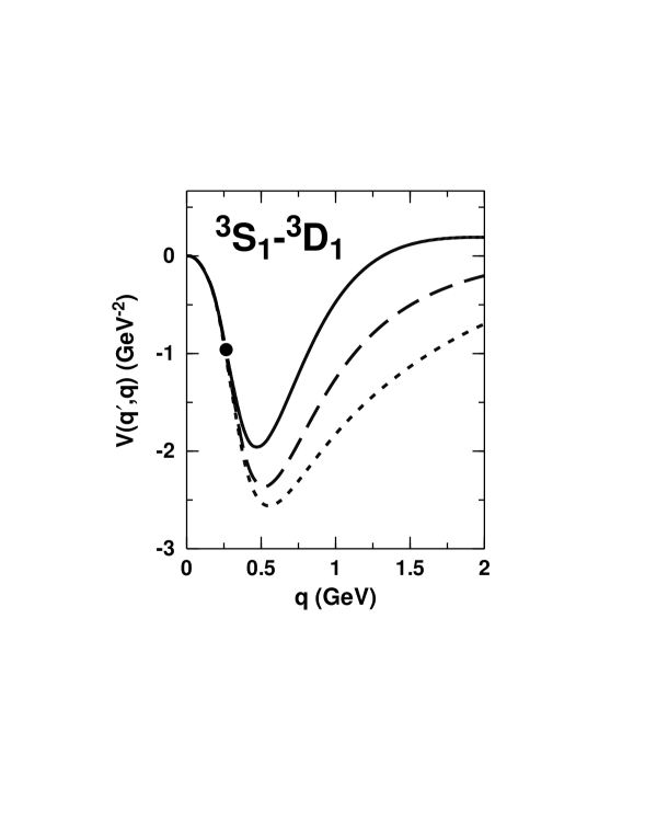
FIG. 2.: Half off-shell ${}^{3}S_{1}$$-$${}^{3}D_{1}$ potential. The on-shell momentum $q^{\prime}$ is held fixed at 265 MeV (equivalent to 150 MeV lab. energy), while the off-shell momentum $q$ runs from zero to 2000 MeV. The on-shell point ($q=265$ MeV) is marked by a solid dot. The solid curve is the relativistic OBE amplitude of $\pi+\rho$ exchange. When the relativistic OPE amplitude, Eq. (10), is replaced by the static/local approximation, Eq. (11), the dashed curve is obtained, and when this approximation is also used for the one-$\rho$ exchange, the dotted curve results.

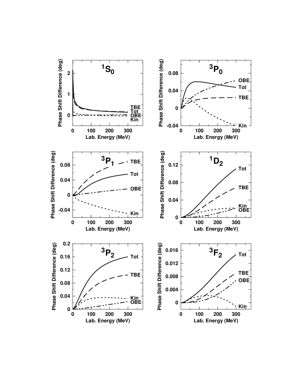
FIG. 3.: Differences $\delta_{nn}-\delta_{pp}$ due to the impact of nucleon mass splitting on kinematics (dotted line labeled ‘Kin’), one-boson exchange diagrams (dashed double-dotted, OBE), and two-boson exchanges (dashed, TBE). The solid line (‘Tot’) represents the total. Notice that each frame has a different scale.

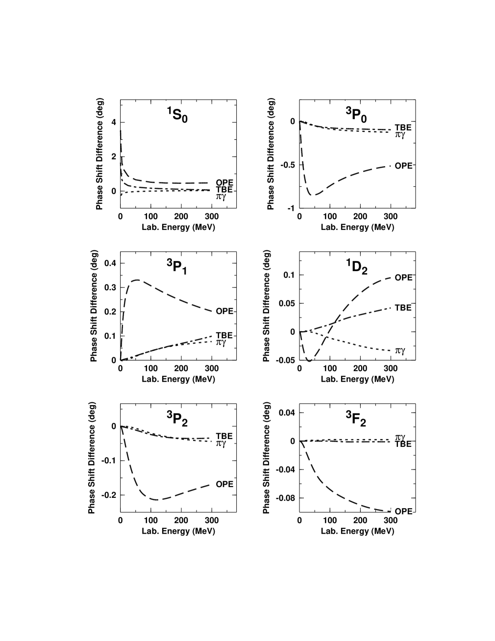
FIG. 4.: Differences $\delta_{np}-\delta_{pp}$ as produced by various CIB mechanisms. Shown are the contributions from OPE (dashed curve), TBE (dashed-dotted), and irreducible $\pi\gamma$ exchange (dotted).

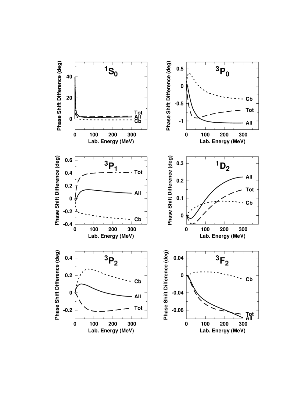
FIG. 5.: The difference $\delta_{np}-\delta_{pp}$ due to the charge-dependence of the strong force (dashed curve labeled ‘Tot’) and $(\delta_{pp}-\delta_{pp}^{C})$ due to the Coulomb force (dotted, Cb). The sum of both is represented by the solid line labeled ‘All’.

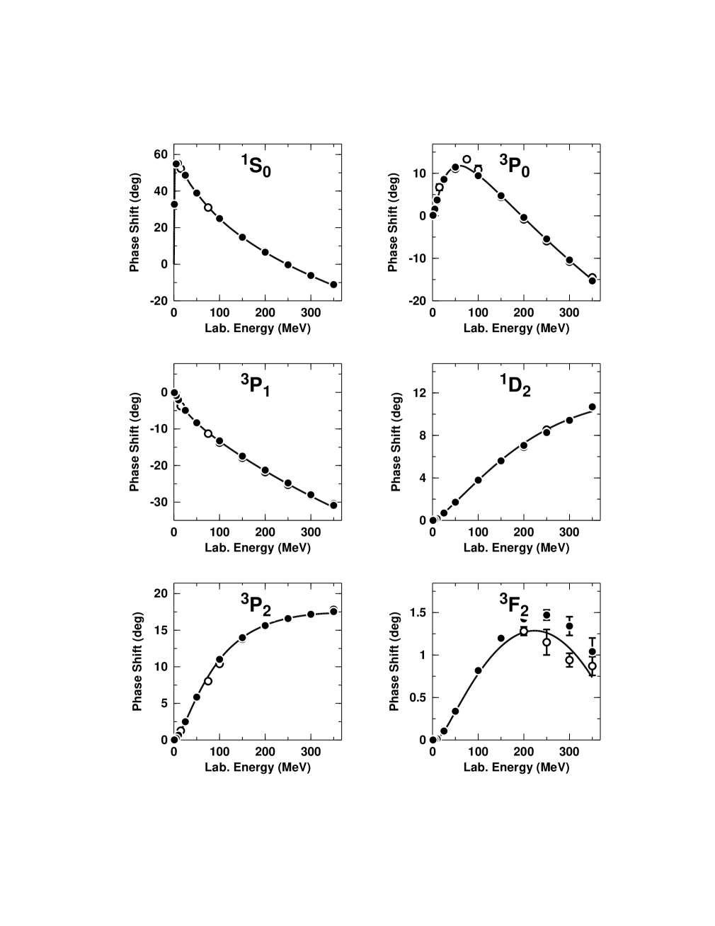
FIG. 6.: $pp$ phase parameters in partial waves with $J\leq 4$. The solid line represents the predictions by the CD-Bonn potential. The solid dots and open circles are the results from the Nijmegen multi-energy $pp$ phase shift analysis [42] and the VPI single-energy $pp$ analysis SM99 [45], respectively.

Fig. 6 continued.

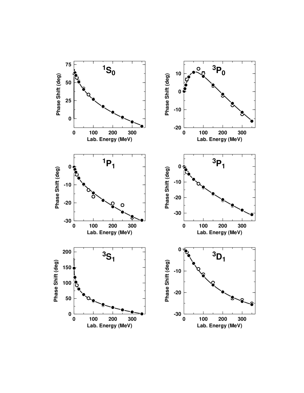
FIG. 7.: $np$ phase parameters in partial waves with $J\leq 4$. The solid line represents the predictions by the CD-Bonn potential. The solid dots and open circles are the results from the Nijmegen multi-energy $np$ phase shift analysis [42] and the VPI single-energy $np$ analysis SM99 [45], respectively.

Fig. 7 continued.

Fig. 7 continued.

Fig. 7 continued.

FIG. 8.: Deuteron wave functions. The family of large curves are $u(r)$ and the family of small curves are $w(r)$. The solid lines represent the wave functions generated from the CD-Bonn potential, while the dashed and dotted lines are from the Nijmegen-I [31] and Argonne $V_{18}$ [32] potentials, respectively.

FIG. 9.: The deuteron wave functions of Fig. 8 in an alternative representation. The family of large curves are $\textstyle u(r)/r$ and the family of small curves are $\textstyle w(r)/r$.

REFERENCES

- [1] R. Machleidt, K. Holinde, and Ch. Elster, Phys. Rep. 149, 1 (1987).
- [2] R. Machleidt, Adv. Nucl. Phys. 19, 189 (1989).
- [3] G. Q. Li and R. Machleidt, Phys. Rev. C 58, 1393 (1998).
- [4] J. A. Nolen and J. P. Schiffer, Annu. Rev. Nucl. Sci. 19, 471 (1969).
- [5] H. Müther, A. Polls, and R. Machleidt, Phys. Lett. B445, 259 (1999).
- [6] G. Q. Li and R. Machleidt, Phys. Rev. C 58, 3153 (1998).
- [7] R. Machleidt, Brueckner theory of nuclear matter with nonnucleonic degrees of freedom and relativity, Advances in Quantum Many-Body Theory, Vol. 3 (World Scientific, Singapore) in press; nucl-th/9911059.
- [8] Review of Particle Physics, Eur. Phys. J. C 3, 1 (1998).
- [9] R. Machleidt, F. Sammarruca, and Y. Song, Phys. Rev. C 53, R1483 (1996).
- [10] W. Grein and P. Kroll, Nucl. Phys. A338, 332 (1980).
- [11] L. Tiator, C. Bennhold, S. S. Kamalov, Nucl. Phys. A580, 455 (1994); M. Kirchbach and L. Tiator, Nucl. Phys. A604, 385 (1996).
- [12] V. Stoks, R. Timmermans, and J. J. de Swart, Phys. Rev. C 47, 512 (1993).
- [13] R. G. E. Timmermans, Few-Body Systems Suppl. 9, 169 (1995); Newsletter 13, 80 (1997); Nucl. Phys. A631, 343c (1998).
- [14] R. A. Arndt, I. I. Strakovsky, and R. L. Workman, Phys. Rev. C 50, 2731 (1994); ibid. 52, 2246 (1995).
- [15] R. A. Arndt, R. L. Workman, and M. M. Pavan, Phys. Rev. C 49, 2729 (1994).
- [16] M. M. Pavan, R. A. Arndt, I. I. Strakovsky, and R. L. Workman, Determination of the Pion-Nucleon Coupling Constant in the VPI/GW Pion-Nucleon Elastic Scattering Partial Wave and Dispersion Relation Analyis, Physica Scripta, in press; nucl-th/9910040.
- [17] R. Machleidt, How sensitive are various observables to changes in the coupling constant?, Physica Scripta, in press; nucl-th/9909036.
- [18] R. Machleidt and M. K. Banerjee, Few-Body Systems, in press; nucl-th/9908066.
- [19] We use the notation and conventions of J. D. Bjorken and S. D. Drell, Relativistic Quantum Mechanics (McGraw-Hill, New York, 1964); moreover—throughout this paper—we use units such that .
- [20] R. Blankenbecler and R. Sugar, Phys. Rev. 142, 1051 (1966).
- [21] E. E. Salpeter and H. A. Bethe, Phys. Rev. 84, 1232 (1951).
- [22] R. Machleidt, Nuclear Forces and Nuclear Structure, Proc. Nuclear Structure 98, Gatlinburg, Tennessee, 1998, AIP Conf. Proc. 481, edited by C. Baktash (AIP, Woodbury, N.Y., 1999) p. 3.
- [23] G. A. Miller and W. H. T. van Oers, In Symmetries and Fundamental Interactions in Nuclei, W. C. Haxton and E. M. Henley, eds. (World Scientific, Singapore, 1995) p. 127.
- [24] G. A. Miller, M. K. Nefkens, and I. Slaus, Phys. Rep. 194, 1 (1990).
- [25] C. R. Howell et al., Phys. Lett. B444, 252 (1998).
- [26] D. E. González Trotter et al., Phys. Rev. Lett. 83, 3788 (1999).
- [27] T.L. Houk, Phys. Rev. C 3, 1886 (1971); W. Dilg, Phys. Rev. C 11, 103 (1975); L. Koester and W. Nistler, Z. Physik A272, 189 (1975); S. Klarsfeld, J. Martorell, and D.W.L. Sprung, J. Phys. G: Nucl. Phys. 10, 165 (1984). For , , and , we use the values recommended by Klarsfeld et al. based upon their own analysis of the experimental results given in the first three references. For , we use the value that is implied by the Klarsfeld analysis. Based upon Refs. [28, 29], we assume fm. ‘Empirical’ values for the are given by Dilg (from which we quote ); however, note that these values are highly model dependent, since the two experimental quantities that the analysis is based upon (namely, the total cross section at ‘zero’ energy and the coherent scattering length) determine only the two scattering lengths and not the effective ranges. A better way to determine the effective ranges is to simply use the predictions from modern high-precision potentials which reproduce the empirical values for the scattering lengths accurately (like the CD-Bonn).
- [28] O. Dumbrajs, R. Koch, H. Pilkuhn, G. C. Oades, H. Behrens, J. J. de Swart, and P. Kroll, Nucl. Phys. B216, 277 (1983).
- [29] J.J. de Swart, C.P.F. Terheggen, and V.G.J. Stoks, The Low-Energy np Scattering Parameters and the Deuteron, University of Nijmegen preprint (1995); nucl-th/9509032.
-
[30]
There are two kinematical effects associated with nucleon
mass splitting that affect the calculation of phase shifts.
These effects are understood most
easily in terms of the radial Schrödinger equation
where denotes the radial wave function, the nucleon mass, and the orbital angular momentum. For scattering and for scattering . This affects the potential term in the above equation, making it stronger in scattering where the larger neutron mass, , is used (this is sometimes called the kinetic energy effect). Besides this, there is a kinematical effect that derives from the fact that the c.m. momentum is given by . Thus, for the same , the c.m. momentum is larger for scattering as compared to . Both effects cause small difference in the phase shifts. Numbers listed in column ‘Kinematics’ of Table III include both effects. - [31] V. G. J. Stoks, R. A. M. Klomp, C. P. F. Terheggen, and J. J. de Swart, Phys. Rev. C 49, 2950 (1994).
- [32] R. B. Wiringa, V. G. J. Stoks, and R. Schiavilla, Phys. Rev. C 51, 38 (1995).
- [33] T. Goldman, J. A. Henderson, and A. W. Thomas, Few-Body Systems 12, 193 (1992).
- [34] J. Piekarewicz and A. G. Williams, Phys. Rev. C 47, 2462 (1993).
- [35] G. Krein, A. W. Thomas, and A. G. Williams, Phys. Lett. B317, 293 (1993).
- [36] H. B. O’Connell, B. C. Pearce, A. W. Thomas, A. G. Williams, Phys. Lett. B336, 1 (1994).
- [37] S. A. Coon, B. H. J. McKellar, and A. A. Rawlinson, in Intersections between Nuclear and Particle Physics, AIP Conf. Proc. 412, edited by T. W. Donelly (AIP, Woodbury,N.Y., 1997), p. 368.
- [38] H. B. O’Connell, B. C. Pearce, A. W. Thomas, A. G. Williams, Prog. Part. Nucl. Phys. 39, 201 (1997).
- [39] S. A. Coon and M. D. Scadron, Charge symmetry breaking via group theory or by the - quark mass difference and direct photon exchange, Proc. XXIII Symposium on Nuclear Physics, Oaxtepec, Mexico, January 2000, Revista Mexicana de Fisica, to be published.
- [40] U. van Kolck, M. C. M. Rentmeester, J. L. Friar, T. Goldman, and J. J. de Swart, Phys. Rev. Lett. 80, 4386 (1998).
- [41] Naively one would expect that the contribution to the difference is exactly of the total CSB phase shift difference due to nucleon mass splitting as listed in Table III. However, there is also a kinematical effect involved that derives from the fact that the correctly calculated c.m. on-shell momentum for scattering [cf. Eq. (A78)] is not the average of the correspnding c.m. momenta for and scattering (obtained for the same ).
- [42] V. G. J. Stoks, R. A. M. Klomp, M. C. M. Rentmeester, and J. J. de Swart, Phys. Rev. C 48, 792 (1993).
- [43] The entries OPE and TBE in Tables V and VI are the predictions by the revised Bonn Full Model (that uses instead of 14.4). These predictions are typically about 5% smaller than what was reported in Ref. [6].
- [44] V. Stoks and J. J. de Swart, Phys. Rev. C 47, 761 (1993).
- [45] R. A. Arndt, I. I. Strakovsky, and R. L. Workman, SAID, Scattering Analysis Interactive Dial-in computer facility, Virginia Polytechnic Institute and George Washington University, solution SM99 (Summer 1999); see also Ref. [14].
- [46] J. R. Bergervoet, P. C. van Campen, W. A. van der Sanden, and J. J. de Swart, Phys. Rev. C 38, 15 (1988).
- [47] V. G. J. Stoks, privat communication.
- [48] W. A. van der Sanden, A. H. Emmen, and J. J. de Swart, Report No. THEF-NYM-83.11, Nijmegen, 1983, unpublished; quoted in Ref. [46].
- [49] J. R. Bergervoet, P. C. van Campen, R. A. M. Klomp, J.-L. de Kok, T. A. Rijken, V. G. J. Stoks, and J. J. de Swart, Phys. Rev. C 41, 1435 (1990).
- [50] W. Kretschmer et al., Phys. Lett. B328, 5 (1994).
- [51] F. Rathmann et al., Phys. Rev. C 58, 658 (1998).
- [52] B. Lorentz, Ph.D. thesis, University of Wisconsin-Madison (1998); B. Lorentz et al., Phys. Rev. C 61, 054002 (2000).
- [53] W. Haeberli et al., Phys. Rev. C 55, 597 (1997).
- [54] S. W. Wissink et al., Phys. Rev. Lett. 83, 4498 (1999).
- [55] B. v. Przewoski et al., Phys. Rev. C 58, 1897 (1998).
- [56] H. Dombrowski, A. Khoukaz, and R. Santo, Nucl. Phys. A619, 97 (1997).
- [57] W. S. Wilburn, C. R. Gould, D. G. Haase, P. R. Huffman, C. D. Keith, N. R. Roberson, and W. Tornow, Phys. Rev. C 52, 2351 (1995).
- [58] B. W. Raichle, C. R. Gould, D. G. Haase, M. L. Seely, J. R. Walston, W. Tornow, W. S. Wilburn, S. I. Penttilä, and G. W. Hoffman, Phys. Rev. Lett. 83, 2711 (1999).
- [59] W. Buerkle and G. Mertens, Few-Body Systems 22, 11 (1997).
- [60] P. Clotten, P. Hempen, K. Hofenbitzer, V. Huhn, W. Metschulat, M. Schwindt, L. Wätzold, Ch. Weber, and W. von Witsch, Phys. Rev. C 58, 1325 (1998).
- [61] J. Brož et al., Z. Physik A354, 401 (1996).
- [62] J. Brož et al., Z. Physik A359, 23 (1997).
- [63] C. A. Davis et al., Phys. Rev. C 53, 2052 (1996).
- [64] A. Ahmidouch et al., Eur. Phys. J. C2, 627 (1998).
- [65] J. Ball et al., Nucl. Phys. A559, 489 (1993).
- [66] J. Ball et al., Nucl. Phys. A574, 697 (1994).
- [67] J. Goetz et al., Nucl. Phys. A574, 467 (1994).
- [68] S. Benck, I. Slypen, V. Corcalciuc, and J.-P. Meulders, Nucl. Phys. A615, 220 (1997).
- [69] J. Rahm et al., Phys. Rev. C 57, 1077 (1998).
- [70] J. Franz, E. Rössle, H. Schmitt, and L. Schmitt, Physica Scripta, in press.
- [71] Proc. Int. Workshop on Critical Points in the Determination of the Pion-Nucleon Coupling Constant, Uppsala (Sweden), June 1999, Physica Scripta, in press.
- [72] C. van der Leun and C. Alderlisten, Nucl. Phys. A380, 261 (1982).
- [73] T.E.O. Ericson and M. Rosa-Clot, Nucl. Phys. A405, 497 (1983).
- [74] N.L. Rodning and L.D. Knutson, Phys. Rev. C 41, 898 (1990).
- [75] F. Schmidt-Kaler, D. Leibfried, M. Weitz, and T.W. Hänsch, Phys. Rev. Lett. 70, 2261 (1993); K. Pachucki, M. Weitz, and T.W. Hänsch, Phys. Rev. A 49, 2255 (1994); J. Martorell, D.W.L. Sprung, and D.C. Zheng, Phys. Rev. C 51, 1127 (1995).
- [76] D.M. Bishop and L.M. Cheung, Phys. Rev. A 20, 381 (1979).
- [77] H. Henning (University of Hannover), privat communication.
- [78] R. Machleidt and F. Sammarruca, Phys. Rev. Lett. 66, 564 (1991).
- [79] A. Polls, H. Müther, R. Machleidt, and M. Hjorth-Jensen, Phys. Lett. B432, 1 (1998).
- [80] H. Arenhövel, F. Ritz, and T. Wilbois, Phys. Rev. C 61, 034002 (2000).
- [81] D. Abbott et al., Phys. Rev. Lett. 84, 5053 (2000).
- [82] D. R. Phillips, S. J. Wallace, and N. K. Devine, nucl-th/9906086. The result of this calculation is represented by the short-dashed curve in Fig. 1 of Ref. [81].
- [83] J. Carbonell and V. A. Karmanov, Eur. Phys. J. A 6, 9 (1999). The result of this calculation is represented by the long-dashed curve in Fig. 1 of Ref. [81].
- [84] L. Engvik, M. Hjorth-Jensen, R. Machleidt, H. Müther, and A. Polls, Nucl. Phys. A627, 85 (1997).
- [85] J. L. Friar et al., Phys. Lett, B311, 4 (1993).
- [86] A. Nogga, H. Kamada, and W. Glöckle, Modern nuclear force predictions for the particle, University of Bochum preprint (2000), nucl-th/0004023.
- [87] P. Navratil, G. P. Kamuntavicius, and B. R. Barrett, Phys. Rev. C 61, 044001 (2000).
- [88] F. Sammarruca, D. P. Xu, and R. Machleidt, Phys. Rev. C 46, 1636 (1992).
- [89] G. Rupp and J. A. Tjon, Phys. Rev. C 45, 2133 (1992).
- [90] F. Sammarruca and R. Machleidt, Few-Body Systems 24, 87 (1998).
- [91] P. J. Siemens and A. P. Vischer, Ann. Phys. (N.Y.) 238, 129, 167 (1995).
- [92] M. F. Jiang, R. Machleidt, D. B. Stout, and T. T. S. Kuo, Phys. Rev. C 46, 910 (1992).
- [93] F. Andreozzi, L. Coraggio, A. Covello, A. Gargano, T. T. S. Kuo, Z. B. Li, and A. Porrino, Phys. Rev. C 54, 1636 (1996); F. Andreozzi, L. Coraggio, A. Covello, A. Gargano, T. T. S. Kuo, and A. Porrino, ibid. 56, R16 (1997), ibid. 59, 746 (1999); L. Coraggio, A. Covello, A. Gargano, N. Itaco, and T. T. S. Kuo, ibid. 60, 064306 (1999); nucl-th/0002021.
- [94] J. Suhonen, J. Toivanen, A. Holt, T. Engeland, E. Osnes, and M. Hjorth-Jensen, Nucl. Phys. A628, 41 (1998); A. Holt, T. Engeland, M. Hjorth-Jensen, and E. Osnes, ibid. A634, 41 (1998).
- [95] A user-friendly computer code for the CD-Bonn potential can be obtained from the author upon request.
- [96] F. Gross, Phys. Rev. C 26, 2203 (1982).
- [97] R. Woloshyn and A. D. Jackson, Nucl. Phys. B64, 269 (1973).
- [98] G. E. Brown, A. D. Jackson, and T. T. S. Kuo, Nucl. Phys. A133, 481 (1969).
- [99] M. Jacob and G. C. Wick, Ann. Phys. (N.Y.) 7, 404 (1959).
- [100] K. Erkelenz, R. Alzetta, and K. Holinde, Nucl. Phys. A176, 413 (1971).
- [101] M. Haftel and F. Tabakin, Nucl. Phys. A158, 1 (1970).
- [102] R. Machleidt, in Computational Nuclear Physics 2—Nuclear Reactions, K. Langanke, J.A. Maruhn, and S.E. Koonin, eds. (Springer, New York, 1993), Chapter 1, pp. 1–29.
- [103] J. Blatt and L. Biedenharn, Phys. Rev. 86, 399 (1952).
- [104] H. P. Stapp, T. J. Ypsilantis, and N. Metropolis, Phys. Rev. 105, 302 (1957).
- [105] M. Abramowitz and I. A. Stegun, Handbook of Mathematical Functions (Dover Publications, New York, 1970).
- [106] G. Breit, Phys. Rev. 99, 1581 (1955).
- [107] G. J. M. Austin and J. J. de Swart, Phys. Rev. Lett. 50, 2039 (1983).
- [108] C. M. Vincent and S. C. Phatak, Phys. Rev. C 10, 391 (1974).
- [109] K. Holinde and R. Machleidt, Nucl. Phys. A247, 495 (1975).
- [110] M. Lacombe, B. Loiseau, J. M. Richard, R. Vinh Mau, J. Côté, P. Pires, and R. de Tourreil, Phys. Lett. B101, 139 (1981).