JLAB-THY-00-15
Weak proton capture on 3He
Abstract
The astrophysical -factor for the proton weak capture on 3He is calculated with correlated-hyperspherical-harmonics bound and continuum wave functions corresponding to realistic Hamiltonians consisting of the Argonne or Argonne two-nucleon and Urbana-VIII or Urbana-IX three-nucleon interactions. The nuclear weak charge and current operators have vector and axial-vector components, that include one- and many-body terms. All possible multipole transitions connecting any of the He S- and P-wave channels to the 4He bound state are considered. The -factor at a He center-of-mass energy of keV, close to the Gamow-peak energy, is predicted to be keV b with the AV18/UIX Hamiltonian, a factor of 4.5 larger than the value adopted in the standard solar model. The P-wave transitions are found to be important, contributing about 40 % of the calculated -factor. The energy dependence is rather weak: the AV18/UIX zero-energy -factor is keV b, only 5 % smaller than the 10 keV result quoted above. The model dependence is also found to be weak: the zero-energy -factor is calculated to be keV b with the older AV14/UVIII model, only 6 % larger than the AV18/UIX result. Our best estimate for the -factor at 10 keV is therefore keV b, when the theoretical uncertainty due to the model dependence is included. This value for the calculated -factor is not as large as determined in fits to the Super-Kamiokande data in which the flux normalization is free. However, the precise calculation of the -factor and the consequent absolute prediction for the neutrino flux will allow much greater discrimination among proposed solar neutrino oscillation solutions.
pacs:
21.45.+v, 27.10.+h, 95.30.CqI Introduction and Conclusions
A Motivation
Recently, there has been a revival of interest in the reaction 3He(,)4He [1, 2, 3, 4, 5, 6]. This interest has been spurred by the Super-Kamiokande collaboration measurements of the energy spectrum of electrons recoiling from scattering with solar neutrinos [7, 8, 9]. Over most of the spectrum, a suppression is observed relative to the Standard Solar Model (SSM) predictions [10]. Above 12.5 MeV, however, there is an apparent excess of events. The process, as the proton weak capture on 3He is known, is the only source of solar neutrinos with energies larger than about 14 MeV–their end-point energy is about 19 MeV. This fact has naturally led to questions about the reliability of calculations of the weak capture cross section, upon which is based the currently accepted SSM value for the astrophysical -factor at zero energy, keV b [11]. In particular, Bahcall and Krastev have shown [1] that a large enhancement, by a factor in the range 25–30, of the SSM -factor value given above would essentially fit the observed excess [7] of recoiling electrons, in any of three different neutrino scenarios–uniform suppression of the 8B flux, vacuum oscillations, and matter-enhanced oscillations [12].
The theoretical description of the process, as well as that of the neutron and proton radiative captures on 2H, 3H, and 3He, constitute a challenging problem from the standpoint of nuclear few-body theory. Its difficulty can be appreciated by comparing the measured values for the cross section of thermal neutron radiative capture on 1H, 2H, and 3He. Their respective values are: mb [13], mb [14], and mb [15, 16]. Thus, in going from =2 to 4 the cross section has dropped by almost four orders of magnitude. These processes are induced by magnetic-dipole transitions between the initial two-cluster state in relative S-wave and the final bound state. In fact, the inhibition of the =3 and 4 captures has been understood for a long time [17]. The 3H and 4He wave functions, denoted, respectively, with and are, to a good approximation, eigenfunctions of the magnetic dipole operator , namely and , where =2.793 n.m. is the proton magnetic moment (note that the experimental value of the 3H magnetic moment is 2.979 n.m., while 4He has no magnetic moment). These relations would be exact, if the 3H and 4He wave functions were to consist of a symmetric S-wave term only, for example, . Of course, tensor components in the nuclear interactions generate significant D-state admixtures, that partially spoil this eigenstate property. To the extent that it is approximately satisfied, though, the matrix elements and vanish due to orthogonality between the initial and final states. This orthogonality argument fails in the case of the deuteron, since then
| (1) |
where and are two-nucleon spin and isospin states, respectively. The magnetic dipole operator can therefore connect the large S-wave component of the deuteron to a =1 1S0 state (note that the orthogonality between the latter and the deuteron follows from the orthogonality between their respective spin-isospin states).
This quasi-orthogonality, while again invalid in the case of the proton weak capture on protons, is also responsible for inhibiting the process. Both these reactions are induced by the Gamow-Teller operator, which differs from the (leading) isovector spin part of the magnetic dipole operator essentially by an isospin rotation. As a result, the weak capture and , , He, and H radiative captures are extremely sensitive to: (i) small components in the wave functions, particularly the D-state admixtures generated by tensor interactions, and (ii) many-body terms in the electro-weak current operator. For example, two-body current contributions provide, respectively, 50 % and over 90 % of the calculated [18] and He [11, 19] cross sections at very low energies.
In this respect, the weak capture is a particularly delicate reaction, for two additional reasons: firstly and most importantly, the one- and two-body current contributions are comparable in magnitude, but of opposite sign [11, 20]; secondly, two-body axial currents, specifically those arising from excitation of isobars which have been shown to give the dominant contribution, are model dependent [20, 21, 22].
This destructive interference between one- and two-body currents also occurs in the He (“”) radiative capture [11, 19], with the difference that there the leading components of the two-body currents are model independent, and give a much larger contribution than that associated with the one-body current.
The cancellation in the process between the one- and two-body matrix elements has the effect of enhancing the importance of P-wave capture channels, which would ordinarily be suppressed. Indeed, one of the results of the present work is that these channels give about 40 % of the -factor calculated value. That the process could proceed as easily through P- as S-wave capture was not realized–or, at least, not sufficiently appreciated [23]–in all earlier studies of this reaction we are aware of, with the exception of Ref. [4], where it was suggested, on the basis of a very simple one-body reaction model, that the 3P0 channel may be important.
B Previous Studies of the Capture
The history of cross section calculations has been most recently reviewed by Bahcall and Krastev [1]. The first estimate of the cross section [24] was based on the calculation of the overlap of an s-wave proton continuum wave function and a 1s neutron wave function in 4He. It produced a large value for the -factor, keV b, and led to the suggestion by Kuzmin [25] that between 20 % and 50 % of the neutrinos in the high-energy end of the flux spectrum could originate from the reaction. Of course, as already discussed above and originally pointed out by Werntz and Brennan [26], if the 4He and He states are approximated, respectively, by (1s)4 and (1s)32sc configurations (2sc is the continuum wave function), and antisymmetrized in space, spin, and isospin, then the capture rate vanishes identically. Werntz and Brennan [26] attempted to relate the matrix element of the axial current occurring in the capture to that of the electromagnetic current occurring in the thermal neutron radiative capture on 3He, and provided an upper limit for the -factor, keV b, based on an experimental upper limit of 100 b for the 3He(,)4He cross section known at the time.
Werntz and Brennan assumed: (i) the validity of isospin symmetry, apart from differences in the neutron (in capture) and proton (in capture) continuum wave functions, which they related to each other via ( is the usual Gamow penetration factor); (ii) that two-body currents dominated both the weak and radiative captures, and that their matrix elements could be put in relation to each other through an isospin rotation. These authors refined their earlier estimate for the -factor in a later publication [23], by using hard-sphere phase shifts to obtain a more realistic value for the ratio of the neutron to proton continuum wave functions, and by including the contributions due to P-wave capture channels. These refinements led to an -factor value, keV b, considerably larger than they had obtained previously. They found, though, that the P-waves only contribute at the 10 % level.
Subsequent studies of the process also attempted to relate it to the radiative capture, but recognized the importance of D-state components in the 3He and 4He wave functions–these had been ignored in Refs. [23, 26]–, and used the Chemtob-Rho prescription [21] (with some short-range modification) for the two-body terms in the electroweak current operator. Tegnér and Bargholtz [27] and Wervelman et al. [16] found, using a shell-model description of the initial and final states, that two-body current contributions do not dominate the capture processes, in sharp contrast with the assumptions of Refs. [23, 26] and the later conclusions of Refs. [11, 19, 20]. These two groups as well as Wolfs et al. [15] arrived, nevertheless, to contradictory results, due to the different values calculated for the ratio of weak to electromagnetic matrix elements. Tegnér and Bargholtz [27] obtained an -factor value of keV b, the spread being due to the uncertain experimental value of the thermal neutron capture cross section before 1983. This prediction was sharpened by Wolfs et al. [15], who measured the cross section precisely. They quoted an -factor value of keV b. Wervelman et al. [16] also measured the cross section, reporting a value of b in excellent agreement with the Wolfs et al. measurement of b, but estimated an -factor in the range keV b. These discrepancies are presumably due to the schematic wave functions used in the calculations.
In an attempt to reduce the uncertainties in the predicted values for both the radiative and weak capture rates, fully microscopic calculations of these reactions were performed in the early nineties [19, 20], based on ground- and scattering-state wave functions obtained variationally from a realistic Hamiltonian with two- and three-nucleon interactions. The main part of the electromagnetic current operator (denoted as “model independent”) was constructed consistently from the two-nucleon interaction model. The less well known (“model dependent”) electroweak currents associated with the excitation of intermediate isobars and with transition couplings, such as the electromagnetic or axial current, were also included. However, it was emphasized that their contribution was to be viewed as numerically uncertain, as very little empirical information is available on their coupling constants and short-range behavior. These studies showed that both the and reactions have large (in the case of the radiative capture, dominant) contributions from two-body currents. Indeed, the values obtained with one-body only and full currents for the -factor (radiative capture cross section) were, respectively, and keV b (6 and 112 b). These results indicated that the common practice of inferring the -factor from the measured radiative capture cross section is bound to be misleading, because of different initial-state interactions in the He and He channels, and because of the large contributions associated with the two-body components of the electroweak current operator, and their destructive interference with the one-body current contributions. Yet, the substantial overprediction of the cross section, 112 b versus an experimental value of 55 b, was unsatisfactory. It became clear that the contributions of the “model dependent”currents, particularly those due to the isobar, were unreasonably large (about 40 b out of the total 112 b). It was therefore deemed necessary to include the degrees of freedom explicitly in the nuclear wave functions, rather than eliminate them in favor of effective two-body operators acting on nucleon coordinates, as it had been done in earlier studies. This led to the development of the transition-correlation operator (TCO) method [11]–a scaled-down approach to a full + coupled-channel treatment. The radiative capture cross section was now calculated to be between 75 and 80 b [11] (excluding the small contribution of the “uncertain” current), the spread depending on whether the coupling constant in the transition interactions is taken either from experiment or from the quark model. In this approach, the -factor was calculated to be in the range between and keV b [11], the spread due to whether the axial coupling was determined by fitting the Gamow-Teller matrix element in tritium -decay or, again, taken from the quark model (uncertainties in the values of the coupling had a much smaller impact). In fact, the SSM value for the -factor now quoted in the literature [1, 2] is the average of these last two results.
C Overview of Present Calculations
Improvements in the modeling of two- and three-nucleon interactions and the nuclear weak current, and the significant progress made in the last few years in the description of the bound and continuum four-nucleon wave functions, have prompted us to re-examine the reaction. The nuclear Hamiltonian has been taken to consist of the Argonne two-nucleon [28] and Urbana-IX three-nucleon [29] interactions. To make contact with the earlier studies [11, 20], however, and to have some estimate of the model dependence of the results, the older Argonne two-nucleon [30] and Urbana-VIII three-nucleon [31] interaction models have also been used. Both these Hamiltonians, the AV18/UIX and AV14/UVIII, reproduce the experimental binding energies and charge radii of the trinucleons and 4He in exact Green’s function Monte Carlo (GFMC) calculations [32, 33].
The correlated-hyperspherical-harmonics (CHH) method is used here to solve variationally the bound- and scattering-state four-nucleon problem [34, 35]. The binding energy of 4He calculated with the CHH method [34, 36] is within 1–2 %, depending on the Hamiltonian model, of that obtained with the GFMC method. The accuracy of the CHH method to calculate scattering states has been successfully verified in the case of the trinucleon systems, by comparing results for a variety of scattering observables obtained by a number of groups using different techniques [37]. Indeed, the numerical uncertainties in the calculation of the trinucleon continuum have been so drastically reduced that scattering observables can now be used to directly study the sensitivity to two- and three-nucleon interaction models–the “puzzle”constitutes an excellent example of this type of studies [38].
Studies along similar lines show [39] that the CHH solutions for the four-nucleon continuum are also highly accurate. The CHH predictions [35] for the H total elastic cross section, , and coherent scattering length, , measured by neutron interferometry techniques– and are the singlet and triplet scattering lengths–have been found to be in excellent agreement with the corresponding experimental values. The H cross section is known over a rather wide energy range, and its extrapolation to zero energy is not problematic [40]. The situation is different for the He channel, for which the scattering lengths have been determined from effective range extrapolations of data taken above 1 MeV, and are therefore somewhat uncertain, fm [41] and fm [41] or fm [27]. Nevertheless, the CHH results are close to the experimental values above. For example, the AV18/UIX Hamiltonian predicts [35] fm and fm.
In Refs. [11, 20] variational Monte Carlo (VMC) wave functions had been used to describe both bound and scattering states. The triplet scattering length was found to be 10.1 fm with the AV14/UVIII Hamiltonian model, in satisfactory agreement with the experimental determination and the value obtained with the more accurate CHH wave functions. However, the present work includes all S- and P-wave channels, namely 1S0, 3S1, 3P0, 1P1, 3P1, and 3P2, while all previous works only retained the 3S1 channel, which was thought, erroneously, to be the dominant one.
The nuclear weak current consists of vector and axial-vector parts, with corresponding one-, two-, and many-body components. The weak vector current is constructed from the isovector part of the electromagnetic current, in accordance with the conserved-vector-current (CVC) hypothesis. Two-body weak vector currents have “model-independent”and “model-dependent”components. The model-independent terms are obtained from the nucleon-nucleon interaction, and by construction satisfy current conservation with it. The leading two-body weak vector current is the “-like”operator, obtained from the isospin-dependent spin-spin and tensor nucleon-nucleon interactions. The latter also generate an isovector “-like”current, while additional isovector two-body currents arise from the isospin-independent and isospin-dependent central and momentum-dependent interactions. These currents are short-ranged, and numerically far less important than the -like current. With the exception of the -like current, they have been neglected in the present work. The model-dependent currents are purely transverse, and therefore cannot be directly linked to the underlying two-nucleon interaction. The present calculation includes the isovector currents associated with excitation of isobars which, however, are found to give a rather small contribution in weak-vector transitions, as compared to that due to the -like current. The -like and -like weak vector charge operators have also been retained in the present study.
The leading two- and many-body terms in the axial current, in contrast to the case of the weak vector (or electromagnetic) current, are those due to -isobar excitation, which are treated within the TCO scheme. This scheme has in fact been extended [42] to include three-body connected terms which were neglected in the earlier work [11]. The axial charge operator includes the long-range pion-exchange term [43], required by low-energy theorems and the partially-conserved-axial-current relation, as well as the (expected) leading short-range terms constructed from the central and spin-orbit components of the nucleon-nucleon interaction, following a prescription due to Riska and collaborators [44].
The largest model dependence is in the weak axial current. To minimize it, the poorly known transition axial coupling constant has been adjusted to reproduce the experimental value of the Gamow-Teller matrix element in tritium -decay. While this procedure is inherently model dependent, its actual model dependence is in fact very weak, as has been shown in Ref. [45]. The analysis carried out there could be extended to the present case.
D Conclusions
We present here a discussion of the results for the astrophysical -factor and their implications for the Super-Kamiokande (SK) solar neutrino spectrum.
1 Results for the -factor
Our results for the astrophysical -factor, defined as
| (2) |
where is the cross section at center-of-mass energy , is the He relative velocity, and is the fine structure constant, are reported in Table I. By inspection of the table, we note that: (i) the energy dependence is rather weak: the value at keV is only about 4 % larger than that at keV; (ii) the P-wave capture states are found to be important, contributing about 40 % of the calculated -factor. However, the contributions from D-wave channels are expected to be very small. We have verified explicitly that they are indeed small in 3D1 capture. (iii) The many-body axial currents associated with excitation play a crucial role in the (dominant) 3S1 capture, where they reduce the -factor by more than a factor of four; thus the destructive interference between the one- and many-body current contributions, first obtained in Ref. [20], is confirmed in the present study, based on more accurate wave functions. The (suppressed) one-body contribution comes mostly from transitions involving the D-state components of the 3He and 4He wave functions, while the many-body contributions are predominantly due to transitions connecting the S-state in 3He to the D-state in 4He, or viceversa.
It is important to stress the differences between the present and all previous studies. Apart from ignoring, or at least underestimating, the contribution due to P-waves, the latter only considered the long-wavelength form of the weak multipole operators, namely, their = limit, where is the magnitude of the momentum transfer. In 3P0 capture, for example, only the -multipole, associated with the weak axial charge, survives in this limit, and the corresponding -factor is calculated to be keV b, including two-body contributions. However, when the transition induced by the longitudinal component of the axial current (via the -multipole, which vanishes at =) is also taken into account, the -factor becomes keV b, because of destructive interference between the and matrix elements (see discussion in Sec. II C). Thus use of the long-wavelength approximation in the calculation of the cross section leads to inaccurate results.
Finally, besides the differences listed above, the present calculation also improves that of Ref. [11] in a number of other important respects: firstly, it uses CHH wave functions, corresponding to the latest generation of realistic interactions; secondly, the model for the nuclear weak current has been extended to include the axial charge as well as the vector charge and current operators. Thirdly, the one-body operators now take into account the relativistic corrections, which had previously been neglected. In 3S1 capture, for example, these terms increase by 25 % the dominant (but suppressed) and matrix elements calculated with the (lowest order) Gamow-Teller operator. These improvements in the treatment of the one-body axial current indirectly affect also the contributions of the -excitation currents, since the transition axial coupling constant is determined by reproducing the Gamow-Teller matrix element in tritium -decay, as discussed in Sec. IV E below.
The chief conclusion of the present work is that the -factor is predicted to be 4.5 times larger than the value adopted in the SSM. This enhancement, while very significant, is smaller than that first suggested in Refs. [1, 3], and then reconsidered by the SK collaboration in Ref. [9]. A discussion of the implications of our results for the SK solar neutrino spectrum is given below.
Even though our result is inherently model dependent, it is unlikely that the model dependence is large enough to accommodate a drastic increase in the value obtained here. Indeed, calculations using Hamiltonians based on the AV18 two-nucleon interaction only and the older AV14/UVIII two- and three-nucleon interactions predict zero energy -factor values of keV b and keV b, respectively. It should be stressed, however, that the AV18 model, in contrast to the AV14/UVIII, does not reproduce the experimental binding energies and low-energy scattering parameters of the three- and four-nucleon systems. The AV14/UVIII prediction is only 6 % larger than the AV18/UIX zero-energy result. This 6 % variation should provide a fairly realistic estimate of the theoretical uncertainty due to the model dependence. It would be very valuable, though, to repeat the present study with a Hamiltonian consisting of the CD-Bonn interaction [46] which, in contrast to the AV14 and AV18 models, has strongly non-local central and tensor components. We would expect the CD-Bonn calculation to predict an -factor value close to that reported here, provided the axial current in that calculation were again constrained to reproduce the known Gamow-Teller matrix element in tritium -decay [45].
To conclude, our best estimate for the -factor at 10 keV c.m. energy is therefore keV b.
2 Effect on the Super-Kamiokande Solar Neutrino Spectrum
Super-Kamiokande (SK) detects solar neutrinos by neutrino-electron scattering. The energy is shared between the outgoing neutrino and scattered electron, leading to a very weak correlation between the incoming neutrino energy and the measured electron energy. The electron angle relative to the solar direction is also measured, which would in principle allow reconstruction of the incoming neutrino energy. However, the kinematic range of the angle is very forward, and is comparable to the angular resolution of the detector. Furthermore, event-by-event reconstruction of the neutrino energy would be prevented by the detector background. Above its threshold of several MeV, SK is sensitive to the 8B electron neutrinos. These have a total flux of cm-2 s-1 in the SSM [10]. While the flux is uncertain to about 15 %, primarily due to the nuclear-physics uncertainties in the 7Be(,)8B cross section, the spectral shape is more precisely known [47].
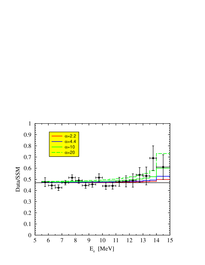
The SK results are presented as the ratio of the measured electron spectrum to that expected in the SSM with no neutrino oscillations. Over most of the spectrum, this ratio is constant at . At the highest energies, however, an excess relative to SSM is seen (though it has diminished in successive data sets). The SK 825-day data, determined graphically from Fig. 8 of Ref. [9], are shown by the points in Fig. 1 (the error bars denote the combined statistical and systematic error). The excess above 12.5 MeV may be interpreted as neutrino-energy dependence in the neutrino oscillation probability that is not completely washed out in the electron spectrum. This excess has also been interpreted as possible evidence for a large flux [1, 3, 9] (though note that the data never exceeds the full SSM expectation from 8B neutrinos). In the SSM, the total flux is very small, cm-2 s-1. However, its endpoint energy is higher than for the 8B neutrinos, 19 MeV instead of about 14 MeV, so that the neutrinos may be seen at the highest energies. This is somewhat complicated by the energy resolution of SK, which allows 8B events beyond their nominal endpoint. The ratio of the flux to its value in the SSM (based on the S-factor prediction of Ref. [11]) will be denoted by , defined as
| (3) |
where is the -neutrino suppression constant. In the present work, , if neutrino oscillations are ignored. The solid lines in Fig. 1 indicate the effect of various values of on the ratio of the electron spectrum with both 8B and to that with only 8B (the SSM). Though some differences are expected in the spectral shape due to P-wave contributions, here we simply use the standard spectrum shape [48]. In calculating this ratio, the 8B flux in the numerator has been suppressed by 0.47, the best-fit constant value for the observed suppression. If the neutrinos are suppressed by , then . Two other arbitrary values of (10 and 20) are shown for comparison. As for the SK data, the results are shown as a function of the total electron energy in 0.5 MeV bins. The last bin, shown covering 14 – 15 MeV, actually extends to 20 MeV. The SK energy resolution was approximated by convolution with a Gaussian of energy-dependent width, chosen to match the SK LINAC calibration data [49].
The effects of a larger flux should be compared to other possible distortions of the ratio. The data show no excess at low energies, thus limiting the size of a neutrino magnetic moment contribution to the scattering [50]. The 8B neutrino energy spectrum has recently been remeasured by Ortiz et al. [51] and their spectrum is significantly larger at high energies than that of Ref. [47]. Relative to the standard spectrum, this would cause an increase in the ratio at high energies comparable to the case. The measured electron spectrum is very steep, and the fraction of events above 12.5 MeV is only of the total above threshold. Thus, an error in either the energy scale or resolution could cause an apparent excess of events at high energy. However, these are known precisely from the SK LINAC [49] calibration; an error in either could explain the data only if it were at about the 3- or 4-sigma level [9].
The various neutrino oscillation solutions can be distinguished by their neutrino-energy dependence, though the effects on the electron spectrum are small. Generally, the ratio is expected to be rising at high energies, much like the effect of an increased flux. The present work predicts (and if the neutrinos oscillate). From Fig. 1, this effect is smaller than the distortion seen in the data or found in Refs. [1, 3, 9], where the flux was fitted as a free parameter. However, the much more important point is that this is an absolute prediction. Fixing the value of will significantly improve the ability of SK to identify the correct oscillation solution.
In the remainder of the paper we provide details of the calculation leading to these conclusions. In Sec. II we derive the cross section in terms of reduced matrix elements of the weak current multipole operators. In Sec. III we discuss the calculation of the bound- and scattering-state wave functions with the CHH method, and summarize a number of results obtained for the 4He binding energy and He elastic scattering observables, comparing them to experimental data. In Sec. IV we review the model for the nuclear weak current and charge operators, while in Sec. V we provide details about the calculation of the matrix elements and resulting cross section. Finally, in Sec. VI we summarize and discuss our results.
II Cross Section
In this section we sketch the derivation of the cross section for the He weak capture process. The center-of-mass (c.m.) energies of interest are of the order of 10 keV–the Gamow-peak energy is 10.7 keV–and it is therefore convenient to expand the He scattering state into partial waves, and perform a multipole decomposition of the nuclear weak charge and current operators. The present study includes S- and P-wave capture channels, i.e. the 1S0, 3S1, 3P0, 1P1, 3P1, and 3P2 states in the notation 2S+1LJ with , and retains all contributing multipoles connecting these states to the =0+ 4He ground state. The relevant formulas are given in the next three subsections. Note that the 1P1 and 3P1, and 3S1 and 3D1 channels are coupled. For example, a pure 1P1 incoming wave will produce both 1P1 and 3P1 outgoing waves. The degree of mixing is significant, particularly for the P-waves, as discussed in Sec. III C.
A The Transition Amplitude
The capture process 3He(,)4He is induced by the weak interaction Hamiltonian [52]
| (4) |
where is the Fermi coupling constant (=1.14939 10-5 GeV-2 [53]), is the leptonic weak current
| (5) |
and is the hadronic weak current density. The positron and (electron) neutrino momenta and spinors are denoted, respectively, by and , and and . The Bjorken and Drell [54] conventions are used for the metric tensor and -matrices. However, the spinors are normalized as .
The transition amplitude in the c.m. frame is then given by
| (6) |
where , and represent the He scattering state with relative momentum and 4He bound state recoiling with momentum , respectively, and
| (7) |
The dependence of the amplitude upon the spin-projections of the proton and 3He is understood. It is useful to perform a partial-wave expansion of the He scattering wave function
| (8) |
with
| (9) |
where and are the proton and 3He spin projections, , , and are the relative orbital angular momentum, channel spin (=0,1), and total angular momentum (), respectively, is the -matrix in channel , and is the Coulomb phase shift,
| (10) | |||||
| (11) |
Here is the fine-structure constant and is the He relative velocity, , being the reduced mass, ( and are the proton and 3He rest masses, respectively). Note that has been constructed to satisfy outgoing wave boundary conditions, and that the spin quantization axis has been chosen to lie along , which defines the -axis. Finally, the scattering wave function as well as the 4He wave function are obtained variationally with the correlated-hyperspherical-harmonics (CHH) method, as described in Sec. III.
The transition amplitude is then written as
| (12) | |||||
| (13) |
where, with the future aim of a multipole decomposition of the weak transition operators, the lepton vector has been expanded as
| (14) |
with and
| (15) | |||||
| (16) |
The orthonormal basis , , is defined by , , .
B The Multipole Expansion
Standard techniques [52] can now be used to perform the multipole expansion of the weak charge and current matrix elements occurring in Eq. (13). The spin quantization axis is along rather than along . Thus, we first express the states quantized along as linear combinations of those quantized along :
| (17) |
where are standard rotation matrices [52, 55] and the angles and specify the direction . We then make use of the transformation properties under rotations of irreducible tensor operators to arrive at the following expressions:
| (18) |
| (19) |
| (20) | |||||
| (21) |
Here , and , , and denote the reduced matrix elements of the Coulomb , longitudinal , transverse electric and transverse magnetic multipole operators, explicitly given by [52]
| (22) |
| (23) |
| (24) |
| (25) |
where are vector spherical harmonics.
Finally, it is useful to consider the transformation properties under parity of the multipole operators. The weak charge/current operators have components of both scalar/polar-vector (V) and pseudoscalar/axial-vector (A) character, and hence
| (26) |
where is any of the multipole operators above. Obviously, the parity of th-pole V-operators is opposite of that of th-pole A-operators. The parity of Coulomb, longitudinal, and electric th-pole V-operators is , while that of magnetic th-pole V-operators is .
C The Cross Section
The cross section for the 3He(,)4He reaction at a c.m. energy is given by
| (28) | |||||
where = 19.287 MeV ( is the 4He rest mass), and is the He relative velocity defined above. It is convenient to write:
| (29) |
where the lepton tensor is defined as
| (30) | |||||
| (31) |
with , and . The nuclear tensor is defined as
| (32) |
where
| (33) |
| (34) |
| (35) |
The dependence upon the direction and proton and 3He spin projections and is contained in the functions given by
| (37) | |||||
with . Note that the Cartesian components of the lepton and nuclear tensors () are relative to the orthonormal basis , , , defined at the end of Sec. II A.
The expression for the nuclear tensor can be further simplified by making use of the reduction formulas for the product of rotation matrices [55]. In fact, it can easily be shown that the dependence of upon the angle can be expressed in terms of Legendre polynomials and associated Legendre functions with . However, given the large number of channels included in the present study (all S- and P-wave capture states), the resulting equations for are not particularly illuminating, and will not be given here. Indeed, the calculation of the cross section, Eq. (28), is carried out numerically with the techniques discussed in Sec. V B.
It is useful, though, to discuss the simple case in which only the contributions involving transitions from the 3S1 and 3P0 capture states are considered. In the limit , one then finds
| (38) |
where and are the longitudinal and transverse electric axial current reduced matrix elements (from 3S1 capture), and is the Coulomb axial charge reduced matrix element (from 3P0 capture) at =0. Here the “Fermi function” is defined as
| (39) |
with . The expression in Eq. (38) can easily be related, mutatis mutandis, to that given in Ref. [20].
Although the =0 approximation can appear to be adequate for the reaction, for which MeV/c and or less ( being the 4He radius), the expression for the cross section given in Eq. (38) is in fact inaccurate. To elaborate this point further, consider the 3P0 capture. The long-wavelength forms of the and multipoles, associated with the axial charge and longitudinal component of the axial current, are constant and linear in , respectively, as can be easily inferred from Eqs. (22)–(23). The corresponding reduced matrix elements are, to leading order in ,
| (40) | |||||
| (41) |
where in the notation of Eq. (38). The 3P0 capture cross section can be written, in this limit, as
| (42) |
When the full model for the nuclear axial charge and current is considered, the constants and , at zero He relative energy, are calculated to be fm3/2 and fm5/2 (note that they are purely imaginary at ). The “Fermi functions”, , and , that arise after integration over the phase space, at have the values , , and . The zero energy -factor obtained by including only the term is 2.2 keV b. However, when both the and terms are retained, it becomes 0.6810-20 keV b.
In fact, this last value is still inaccurate: when not only the leading, but also the next-to-leading order terms are considered in the expansion of the multipoles in powers of (see Sec. V B), the -factor for 3P0 capture increases to 0.8210-20 keV b, its fully converged value. The conclusion of this discussion is that use of the long-wavelength approximation in the reaction leads to erroneous results.
Similar considerations also apply to the case of 3S1 capture: at values of different from zero, the transition can be induced not only by the axial current via the and multipoles, but also by the axial charge and vector current via the and and multipoles. While the contribution of is much smaller than that of the leading and , the contribution of is relatively large, and its interference with that of cannot be neglected. This point is further discussed in Sec. VI B.
As a final remark, we note that the general expression for the cross section in Eq. (28) as follows from Eqs. (29)–(37) contains interference terms among the reduced matrix elements of multipole operators connecting different capture channels. However, these interference contributions have been found to account for less than 2 % of the total -factor at zero He c.m. energy.
III Bound- and Scattering-State Wave Functions
The 4He bound-state and He scattering-state wave functions are obtained variationally with the correlated-hyperspherical-harmonics (CHH) method from realistic Hamiltonians consisting of the Argonne two-nucleon [28] and Urbana-IX three-nucleon [29] interactions (the AV18/UIX model), or the older Argonne two-nucleon [30] and Urbana-VIII three-nucleon [31] interactions (the AV14/UVIII model). The CHH method, as implemented in the calculations reported in the present work, has been developed by Viviani, Kievsky, and Rosati in Refs. [34, 35, 56, 57]. Here, it will be reviewed briefly for completeness, and a summary of relevant results obtained for the three- and four-nucleon bound-state properties, and He effective-range parameters will be presented.
A The CHH Method
In the CHH approach a four-nucleon wave function is expanded as
| (43) |
where the amplitudes and correspond, respectively, to the partitions 3+1 and 2+2, and the index runs over the even permutations of particles . The dependence on the spin-isospin variables is understood. The overall antisymmetry of the wave function is ensured by requiring that both and change sign under the exchange .
The Jacobi variables corresponding to the partition 3+1 are defined as
| (44) | |||||
| (45) | |||||
| (46) |
while those corresponding to the partition 2+2 are defined as
| (47) | |||||
| (48) | |||||
| (49) |
where () and denote the c.m. positions of particles () and , respectively. In the -coupling scheme, the amplitudes and are expanded as
| (50) |
| (51) |
where
| (53) | |||||
| (55) | |||||
Here a channel is specified by: orbital angular momenta , , , , and ; spin angular momenta , , and ; isospins and . The total orbital and spin angular momenta and cluster isospins are then coupled to the assigned and .
The correlation factors consist of the product of pair-correlation functions, that are obtained from solutions of two-body Schrödinger-like equations, as discussed in Ref. [34]. These correlation factors take into account the strong state-dependent correlations induced by the nucleon-nucleon interaction, and improve the behavior of the wave function at small interparticle separations, thus accelerating the convergence of the calculated quantities with respect to the number of required hyperspherical harmonics basis functions, defined below.
The radial amplitudes and are further expanded as
| (56) | |||||
| (57) |
where the magnitudes of the Jacobi variables have been replaced by the hyperspherical coordinates, i.e. the hyperradius
| (58) |
which is independent of the permutation considered, and the hyperangles appropriate for partitions A and . The latter are given by
| (59) | |||||
| (60) | |||||
| (61) |
Finally, the hyperangle functions consist of the product of Jacobi polynomials
| (62) |
where the indices and run, in principle, over all non-negative integers, , and are normalization factors [34].
Once the expansions for the radial amplitudes and are inserted into Eqs. (50)–(51), the wave function can schematically be written as
| (63) |
where and are yet to be determined, and the factors , with , include the dependence upon the hyperradius due to the correlation functions, and the angles and hyperangles, denoted collectively by , and are given by:
| (64) |
B The 3He and 4He Wave Functions
The Rayleigh-Ritz variational principle
| (65) |
is used to determine the hyperradial functions in Eq. (63) and bound state energy . Carrying out the variations with respect to the functions leads to a set of coupled second-order linear differential equations in the variable which, after discretization, is converted into a generalized eigenvalue problem and solved by standard numerical techniques [34].
The present status of 3He [58] and 4He [34, 36] binding energy calculations with the CHH method is summarized in Tables II and III. The binding energies calculated with the CHH method using the AV18 or AV18/UIX Hamiltonian models are within 1.5 % of corresponding “exact”Green’s function Monte Carlo (GFMC) results [32], and of the experimental value (when the three-nucleon interaction is included). The agreement between the CHH and GFMC results is less satisfactory when the AV14 or AV14/UVIII models are considered, presumably because of slower convergence of the CHH expansions for the AV14 interaction. This interaction has tensor components which do not vanish at the origin.
C The He Continuum Wave Functions
The He cluster wave function , having incoming orbital angular momentum and channel spin () coupled to total angular , is expressed as
| (66) |
where the term vanishes in the limit of large intercluster separations, and hence describes the system in the region where the particles are close to each other and their mutual interactions are strong. The term describes the system in the asymptotic region, where intercluster interactions are negligible. It is given explicitly as:
| (68) | |||||
where is the distance between the proton (particle ) and 3He (particles ), is the magnitude of the relative momentum between the two clusters, is the 3He wave function, and and are the regular and irregular Coulomb functions, respectively. The function modifies the at small by regularizing it at the origin, and as fm, thus not affecting the asymptotic behavior of . Finally, the real parameters are the -matrix elements introduced in Eq. (9), which determine phase shifts and (for coupled channels) mixing angles at the energy ( is He reduced mass). Of course, the sum over and is over all values compatible with a given and parity.
The “core”wave function is expanded in the same CHH basis as the bound-state wave function, and both the matrix elements and functions occurring in the expansion of are determined by making the functional
| (69) |
stationary with respect to variations in the and (Kohn variational principle). Here MeV is the 3He ground-state energy. It is important to emphasize that the CHH scheme, in contrast to Faddeev-Yakubovsky momentum space methods, permits the straightforward inclusion of Coulomb distortion effects in the He channel.
The He singlet and triplet scattering lengths predicted by the Hamiltonian models considered in the present work are listed in Table III, and are found in good agreement with available experimental values, although these are rather poorly known. The experimental scattering lengths have been obtained, in fact, from effective range parametrizations of data taken above MeV, and therefore might have large systematic uncertainties.
The most recent determination of phase-shift and mixing-angle parameters for He elastic scattering has been performed in Ref. [41] by means of an energy-dependent phase-shift analysis (PSA), including almost all data measured prior 1993 (for a listing of old PSAs, see Ref. [41]). New measurements are currently under way at TUNL [59] and Madison [60]. At low energies ( MeV) the process is dominated by scattering in = and waves, with a small contribution from = waves. Therefore, the important channels are: 1S0, 3P0, 3S1-3D1, 1P1-3P1, 3P2, 1D2-3D2 and 3D3, ignoring channels with . The general trend is the following: (i) the energy dependence of the S-wave phase shifts indicates that the =0 channel interaction between the and 3He is repulsive (mostly, due to the Pauli principle), while that of the four P-wave phase shifts (3P0, 1P1, 3P1, and 3P2) shows that in these channels there is a strong attraction. Indeed, this fact has led to speculations about the existence of four resonant states [61]. (ii) The D-wave phase shifts are rather tiny, even at MeV. (iii) The only mixing-angle parameter playing an important role at MeV is , in channel 1P1-3P1.
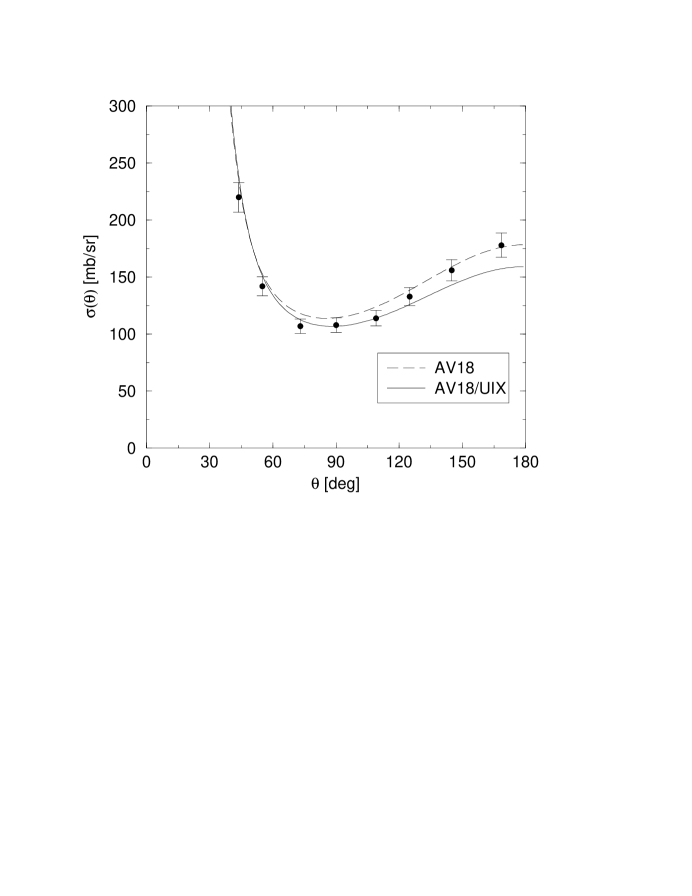
Precise measurements have been taken at a c.m. energy of MeV, and consist in differential cross section [62] and proton analyzing power [60] data ( is the c.m. scattering angle). The theoretical predictions for , obtained from the AV18 and AV18/UIX interactions, are compared with the corresponding experimental data in Fig. 2. Inspection of the figure shows that the differential cross section calculated with the AV18/UIX model is in excellent agreement with the data, except at backward angles.
By comparing, in Table IV, the calculated phase-shift and mixing-angle parameters with those extracted from the PSA [41] at MeV, one observes a qualitative agreement, except for the 3P1 and 3P2 phase shifts which are significantly underestimated in the calculation. The mixing-angle parameter is found to be rather large, , in qualitative agreement with that obtained from the PSA (it is worth pointing out, however, that in the PSA the mixing angle was constrained to vanish at , which may be unphysical). The experimental error for each parameter quoted in Ref. [41] is an average uncertainty over the whole energy range considered, and it is therefore only indicative. It would be very interesting to relate these discrepancies to the puzzle and to specific deficiencies in the nuclear interaction models. A detailed study of He elastic scattering is currently underway and will published elsewhere [63].
IV The Weak Charge and Current Operators
The nuclear weak charge and current operators have scalar/polar-vector (V) and pseudoscalar/axial-vector (A) components
| (70) | |||||
| (71) |
where is the momentum transfer, , and the subscripts denote charge raising (+) or lowering (–) isospin indices. Each component, in turn, consists of one-, two-, and many-body terms that operate on the nucleon degrees of freedom:
| (72) | |||||
| (73) |
where =V, A and the isospin indices have been suppressed to simplify the notation. The one-body operators and have the standard expressions obtained from a non-relativistic reduction of the covariant single-nucleon V and A currents, and are listed below for convenience. The V-charge operator is written as
| (74) |
with
| (75) |
| (76) |
The V-current operator is expressed as
| (77) |
where denotes the anticommutator, , , and are the nucleon’s momentum, Pauli spin and isospin operators, respectively, and is the isovector nucleon magnetic moment ( n.m.). Finally, the isospin raising and lowering operators are defined as
| (78) |
The term proportional to in is the well known [64, 65] spin-orbit relativistic correction. The vector charge and current operators above are simply obtained from the corresponding isovector electromagnetic operators by the replacement , in accordance with the conserved-vector-current (CVC) hypothesis. The -dependence of the nucleon’s vector form factors (and, in fact, also that of the axial-vector form factors below) has been ignored, since the weak transition under consideration here involves very small momentum transfers, MeV/c. For this same reason, the Darwin-Foldy relativistic correction proportional to in has also been neglected. The A-charge operator is given, to leading order, by
| (79) |
while the A-current operator considered in the present work includes leading and next-to-leading order corrections in an expansion in powers of , i.e.
| (80) |
with
| (81) |
| (83) | |||||
The axial coupling constant is taken to be [66] 1.26540.0042, by averaging values obtained, respectively, from the beta asymmetry in the decay of polarized neutrons (1.26260.0033 [67, 68]) and the half-lives of the neutron and superallowed transitions, i.e. =1.26810.0033 [66]. The last term in Eq. (83) is the induced pseudoscalar contribution ( is the muon mass), for which the coupling constant is taken as [69] =–6.78 . As already mentioned in Sec. I, in 3S1 capture matrix elements of are suppressed. Consequently, the relativistic terms included in , which would otherwise contribute at the percent level, give in fact a 20 % contribution relative to that of the leading at =0. Among these, one would naively expect the induced pseudoscalar term to be dominant, due to the relatively large value of . This is not the case, however, since matrix elements of the induced pseudoscalar term scale with ( in the -range of interest) relative to those . Note that in the limit =0, the expressions for and reduce to the familiar Fermi and Gamow-Teller operators.
In the next five subsections we describe: i) the two-body V-current and V-charge operators, required by the CVC hypothesis; ii) the two-body A-current and A-charge operators due to - and -meson exchanges, and the mechanism; iii) the V and A current and charge operators associated with excitation of -isobar resonances, treated in perturbation theory and within the transition-correlation-operator method. Since the expressions for these operators are scattered in a number of papers [11, 20, 70, 71], we collect them here for completeness.
A Two-Body Weak Vector Current Operators
The weak vector (V) current and charge operators are derived from the corresponding electromagnetic operators by making use of the CVC hypothesis, which for two-body terms implies
| (84) |
where are the isovector (charge-conserving) two-body electromagnetic currents, and are isospin Cartesian components. A similar relation holds between the electromagnetic charge operators and its weak vector counterparts. The charge-raising or lowering weak vector current (or charge) operators are then simply obtained from the linear combinations
| (85) |
The two-body electromagnetic currents have “model-independent”(MI) and “model-dependent”(MD) components, in the classification scheme of Riska [72]. The MI terms are obtained from the two-nucleon interaction, and by construction satisfy current conservation with it [70]. Studies of the electromagnetic structure of =2–6 nuclei, such as, for example, the threshold electrodisintegration of the deuteron at backward angles [73], the magnetic form factors of the trinucleons [42], the magnetic dipole transition form factors in 6Li [74], and finally the neutron and proton radiative captures on hydrogen and helium isotopes [19, 73, 75]–properties in which the isovector two-body currents play a large role and are, in fact, essential for the satisfactory description of the experimental data–have shown that the leading operator is the (isovector) “-like”current obtained from the isospin-dependent spin-spin and tensor interactions. The latter also generate an isovector “-like”current. There are additional MI isovector currents, which arise from the central and momentum-dependent interactions, but these are short-ranged and have been found to be numerically far less important than the -like current [70, 73]. Their contributions are neglected in the present study.
Use of the CVC relation leads to the -like and -like weak vector currents below:
| (87) | |||||
| (91) | |||||
where and are the momenta delivered to nucleons and with , the isospin operators are defined as
| (92) |
and , , and are given by
| (93) | |||||
| (94) | |||||
| (95) |
with
| (96) | |||||
| (97) | |||||
| (98) |
Here , , are the isospin-dependent central, spin-spin, and tensor components of the two-nucleon interaction (either the AV14 or AV18 in the present study). The factor in the expression for ensures that its volume integral vanishes. Configuration-space expressions are obtained from
| (99) |
where =V or V. Techniques to carry out the Fourier transforms above are discussed in Ref. [70].
In a one-boson-exchange (OBE) model, in which the isospin-dependent central, spin-spin, and tensor interactions are due to - and -meson exchanges, the functions , , and are simply given by
| (100) | |||||
| (101) | |||||
| (102) |
where and are the meson masses, , and are the pseudovector , vector and tensor coupling constants, respectively, and denote and monopole form factors, i.e.
| (103) |
with = or . For example, in the CD-Bonn OBE model [46] the values for the couplings and cutoff masses are: , , , GeV/c, and GeV/c. Even though the AV14 and AV18 are not OBE models, the functions and, to a less extent, and projected out from their , , and components are quite similar to those of - and -meson exchanges in Eqs. (100)–(102) (with cutoff masses of order 1 GeV/c), as shown in Refs. [70, 75].
Among the MD (purely transverse) isovector currents, those due to excitation of isobars have been found to be the most important, particularly at low momentum transfers, in studies of electromagnetic structure [42] and reactions [11] of few-nucleon systems. Their contribution, however, is still relatively small when compared to that of the leading -like current. Discussion of the weak vector currents associated with degrees of freedom is deferred to Sec. IV E.
B Two-Body Weak Vector Charge Operators
While the main parts of the two-body electromagnetic or weak vector current are linked to the form of the nucleon-nucleon interaction through the continuity equation, the most important two-body electromagnetic or weak vector charge operators are model dependent, and should be viewed as relativistic corrections. Indeed, a consistent calculation of two-body charge effects in nuclei would require the inclusion of relativistic effects in both the interaction models and nuclear wave functions. Such a program is yet to be carried out, at least for systems with .
There are nevertheless rather clear indications for the relevance of two-body electromagnetic charge operators from the failure of the impulse approximation in predicting the deuteron tensor polarization observable [76], and charge form factors of the three- and four-nucleon systems [42, 77]. The model commonly used [71] includes the -, -, and -meson exchange charge operators with both isoscalar and isovector components, as well as the (isoscalar) and (isovector) charge transition couplings (in addition to the single-nucleon Darwin-Foldy and spin-orbit relativistic corrections). The - and -meson exchange charge operators are constructed from the isospin-dependent spin-spin and tensor interactions, using the same prescription adopted for the corresponding current operators [71]. At moderate values of momentum transfer ( fm-1), the contribution due to the “-like”exchange charge operator has been found to be typically an order of magnitude larger than that of any of the remaining two-body mechanisms and one-body relativistic corrections [42].
In the present study we retain, in addition to the one-body operator of Eq. (74), only the “-like”and “-like”weak vector charge operators. In the notation of the previous subsection, these are given by
| (104) |
| (105) | |||||
| (106) |
where non-local terms from retardation effects in the meson propagators or from direct couplings to the exchanged mesons have been neglected [78, 79]. In the operator terms proportional to powers of , because of the large -meson tensor coupling ( 6–7), have also been neglected. Indeed, these terms have been ignored also in most studies of nuclear charge form factors.
C Two-Body Weak Axial Current Operators
In contrast to the electromagnetic case, the axial current operator is not conserved. Its two-body components cannot be linked to the nucleon-nucleon interaction and, in this sense, should be viewed as model dependent. Among the two-body axial current operators, the leading term is that associated with excitation of -isobar resonances. We again defer its discussion to Sec. IV E. In the present section we list the two-body axial current operators due to - and -meson exchanges (the A and A currents, respectively), and the -transition mechanism (the A current). Their individual contributions have been found numerically far less important than those from -excitation currents in studies of weak transitions involving light nuclei [20, 45, 80]. These studies [20, 45] have also found that the A and A current contributions interfere destructively, making their combined contribution almost entirely negligible. These conclusions are confirmed in the present work.
The A, A, and A current operators were first described in a systematic way by Chemtob and Rho [21]. Their derivation has been given in a number of articles, including the original reference mentioned above and the more recent review by Towner [22]. Their momentum-space expressions are given by
| (107) | |||||
| (108) |
| (111) | |||||
| (113) | |||||
where is the sum of the initial and final momenta of nucleon , respectively and , and the functions and have already been defined in Eqs. (100)–(101). Configuration-space expressions are obtained by carrying out the Fourier transforms in Eq. (99). The values used for the and coupling constants and cutoff masses are the following: , , , fm-1, and fm-1. The -meson coupling constants are taken from the older Bonn OBE model [81], rather than from the more recent CD-Bonn interaction [46] ( and ). This uncertainty has in fact essentially no impact on the results reported in the present work for two reasons. Firstly, the contribution from , as already mentioned above, is very small. Secondly, the complete two-body axial current model, including the currents due to -excitation discussed below, is constrained to reproduce the Gamow-Teller matrix element in tritium -decay by appropriately tuning the value of the -transition axial coupling . Hence changes in and only require a slight readjustament of the value.
Finally, note that the replacements and could have been made in the expressions for and above, thus eliminating the need for the inclusion of ad hoc form factors. While this procedure would have been more satisfactory, since it constrains the short-range behavior of these currents in a way consistent with that of the two-nucleon interaction, its impact on the present calculations would still be marginal for the same reasons given above.
D Two-Body Weak Axial Charge Operators
The model for the weak axial charge operator adopted here includes a term of pion-range as well as short-range terms associated with scalar- and vector-meson exchanges [44]. The experimental evidence for the presence of these two-body axial charge mechanisms rests on studies of weak transitions, such as the processes 16N(0-,120 keV)16O(0+) and 16O(0+)+16N(0-,120 keV)+, and first-forbidden -decays in the lead region [82]. Shell-model calculations of these transitions suggest that the effective axial charge coupling of a bound nucleon may be enhanced by roughly a factor of two over its free nucleon value. There are rather strong indications that such an enhancement can be explained by two-body axial charge contributions [44].
The pion-range operator is taken as
| (114) |
where is the pion decay constant (=93 MeV), is the momentum transfer to nucleon , and is the monopole form factor of Eq. (103) with =4.8 fm-1. The structure and overall strength of this operator are determined by soft pion theorem and current algebra arguments [43, 83], and should therefore be viewed as “model independent”. It can also be derived, however, by considering nucleon-antinucleon pair contributions with pseudoscalar coupling.
The short-range axial charge operators can be obtained in a “model-independent”way, consistently with the two-nucleon interaction model. The procedure is described in Ref. [44], and is similar to the one used to derive the “model-independent”electromagnetic or weak vector currents. Here we consider the charge operators associated only with the central and spin-orbit components of the interaction, since these are expected to give the largest contributions, after the operator above. This expectation is in fact confirmed in the present study. The momentum-space expressions are given by
| (115) |
| (117) | |||||
where , and
| (118) |
with =s, s, v, and v. The following definitions have been introduced
| (119) | |||||
| (120) |
where , and are the isospin-independent central, spin-orbit, and components of the AV14 or AV18 interactions, respectively. The definitions for and can be obtained from those above, by replacing the isospin-independent , and with the isospin-dependent , and .
E -Isobar Contributions
In this section we review the treatment of the weak current and charge operators associated with excitation of isobars in perturbation theory and within the context of the transition-correlation-operator (TCO) method [11]. Among the two-body axial current operators, those associated with degrees of freedom have in fact been found to be the most important ones [11, 20].
In the TCO approach, the nuclear wave function is written as
| (121) |
where is the purely nucleonic component, is the symmetrizer, and the transition operators convert pairs into and pairs. The latter are defined as
| (122) |
| (123) | |||||
| (124) |
Here, and are spin- and isospin-transition operators which convert nucleon into a isobar, and are tensor operators in which, respectively, the Pauli spin operators of either particle or , and both particles and are replaced by corresponding spin-transition operators. The vanishes in the limit of large interparticle separations, since no -components can exist asymptotically.
In the present study the is taken from CHH solutions of the AV14/UVIII or AV18/UIX Hamiltonians with nucleons only interactions, while the is obtained from two-body bound and low-energy scattering-state solutions of the full - coupled-channel problem with the Argonne [84] (AV28Q) interaction, containing explicit and degrees of freedom. This aspect of the present calculations, including the validity of the approximation inherent to Eq. (121), were discussed at length in the original work [11], and have been reviewed more recently in Ref. [42], making a further review here unnecessary. The AV28Q interaction provided an excellent description of the database available in the early eighties. No attempt has been made to refit this model to the more recent and much more extensive Nijmegen database [85].
In the TCO scheme, the perturbation theory description of -admixtures is equivalent to the replacements:
| (125) | |||||
| (126) |
where the kinetic energy contributions in the denominators of Eqs. (125) and (126) have been neglected (static approximation). The transition interactions and have the same operator structure as and of Eqs. (123) and (124), but with the and functions replaced by, respectively,
| (127) | |||||
| (128) |
Here = II, III, , , for = II, III, respectively, being the coupling constant, and the cutoff function . In the AV28Q interaction , as obtained in the quark-model, and = 4.09. When compared to , the perturbation theory corresponding to Eqs. (125) and (126) produces and admixtures that are too large at short distances, and therefore leads to a substantial overprediction of the effects associated with isobars in electroweak observables [11].
We now turn our attention to the discussion of and weak transition operators. The axial current and charge operators associated with excitation of isobars are modeled as
| (129) | |||||
| (130) |
and
| (131) | |||||
| (132) |
where is the -isobar mass, () is the Pauli operator for the spin 3/2 (isospin 3/2), and and are defined in analogy to Eq. (78). The expression for () is obtained from that for () by replacing and by their hermitian conjugates. The coupling constants and are not well known. In the quark-model, they are related to the axial coupling constant of the nucleon by the relations and . These values have often been used in the literature in the calculation of -induced axial current contributions to weak transitions. However, given the uncertainties inherent to quark-model predictions, a more reliable estimate for is obtained by determining its value phenomenologically in the following way. It is well established by now [45] that the one-body axial current of Eq. (81) leads to a 4 % underprediction of the measured Gamow-Teller matrix element in tritium -decay, see Table V. Since the contributions of axial currents (as well as those due to the two-body operators of Sec. IV C) are found to be numerically very small, as can be seen again from Table V, this 4 % discrepancy can then be used to determine [86]. Obviously, this procedure produces different values for depending on how the -isobar degrees of freedom are treated. These values are listed in Table VI for comparison. The value that is determined in the context of a TCO calculation based on the AV28Q interaction, is about 40 % larger than the naive quark-model estimate. However, when perturbation theory is used for the treatment of the isobars, the value required to reproduce the Gamow-Teller matrix element of tritium -decay is much smaller than the TCO estimate, as expected. Finally, the axial current derived in perturbation theory from Eqs. (125) and (129) is, of course, identical to the expression given in Refs. [20, 45].
The and weak vector currents are modeled, consistently with the CVC hypothesis, as
| (133) | |||||
| (134) |
where the -transition magnetic moment is taken equal to 3 n.m., as obtained from an analysis of data in the -resonance region [87], while the value used for the magnetic moment is 4.35 n.m. by averaging results of a soft-photon analysis of pion-proton bremsstrahlung data near the resonance [88]. The contributions due to the weak vector currents above have been in fact found to be very small in the He capture process. Finally, to weak vector charge operators are ignored in the present study, since their associated contributions are expected to be negligible.
V Calculation
The calculation of the He weak capture cross section proceeds in two steps: firstly, the Monte Carlo evaluation of the weak charge and current operator matrix elements, and the subsequent decomposition of these in terms of reduced matrix elements; secondly, the evaluation of the cross section by carrying out the integrations in Eq. (28).
A Monte Carlo Calculation of Matrix Elements
In a frame where the direction of the momentum transfer also defines the quantization axis of the nuclear spins, the matrix element of, as an example, the weak axial (or vector) current has the multipole expansion
| (135) |
with . The expansion above is easily obtained from that in Eq. (21), in which the quantization axis for the nuclear spins was taken along the direction of the relative momentum , by setting ==0 and using . Then, again as an example, the reduced matrix element of the axial electric dipole operator involving a transition from the He 3S1 state is simply given by
| (136) |
The problem is now reduced to the evaluation of matrix elements of the same type as on the right-hand-side of Eq. (136). These can schematically be written as
| (137) |
where the initial and final states have the form of Eq. (121). It is convenient to expand the latter as
| (138) |
so that the numerator of Eq. (137) can be expressed as
| (139) |
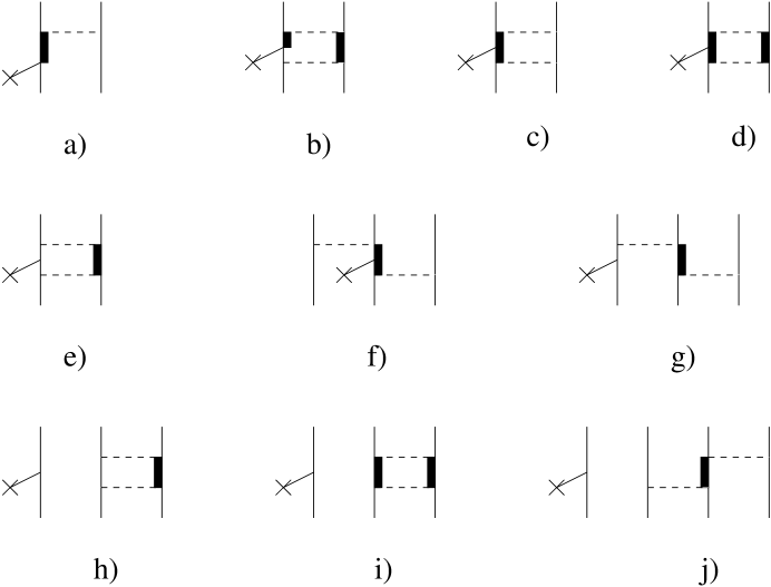
where the operator denotes all one- and two-body contributions to the weak charge or current operator , involving only nucleon degrees of freedom, i.e. , while includes terms that involve the -isobar degrees of freedom, associated with the explicit transitions , , , and with the transition operators . A diagrammatical illustration of the terms contributing to is given in Fig. 3: the terms (a)–(e), (f)–(i), and (j) represent, respectively, two-, three-, and four-body operators. The terms (e) and (g)–(j) are to be viewed as renormalization corrections to the “nucleonic”matrix element of , due to the presence of -admixtures in the wave functions. Connected three-body terms containing more than a single isobar have been ignored, since their contributions are expected to be negligible. Indeed, the contribution from diagram (d) has already been found numerically very small.
The two-body terms of Fig. 3 are expanded as operators acting on the nucleons’ coordinates. For example, the terms (a) and (c) in Fig. 3 have the structure, respectively,
| (140) | |||||
| (141) |
which can be reduced to operators involving only Pauli spin and isospin matrices by using the identities:
| (142) | |||||
| (144) | |||||
where , and are vector operators that commute with , but not necessarily among themselves. While the three- and four-body terms in Fig. 3 could have been reduced in precisely the same way, the resulting expressions in terms of and matrices become too cumbersome. Thus, for these it was found to be more convenient to retain the explicit representation of as a matrix
and of as a matrix
where , , and , and derive the result of terms such as (f)= on state by first operating with , then with , and finally with . These terms (as well as three-body contributions to the wave function normalizations, see below) were neglected in the calculations reported in Ref. [11].
Of course, the presence of -admixtures also influences the normalization of the wave functions, as is obvious from Eq. (137):
| (145) | |||||
| (146) |
The wave function normalization ratios , obtained for the bound three- and four-nucleon systems, are listed in Table VII. Note that the normalization of the He continuum state is the same as that of 3He, up to corrections of order (volume)-1.
The matrix elements in Eqs. (139) and (146) are computed, without any approximation, by Monte Carlo integrations. The wave functions are written as vectors in the spin-isospin space of the four nucleons for any given spatial configuration . For the given we calculate the state vector with the techniques developed in Refs. [42, 70]. The spatial integrations are carried out with the Monte Carlo method by sampling configurations according to the Metropolis et al. algorithm [89], using a probability density proportional to
| (147) |
where the notation implies sums over the spin-isospin states of the 4He wave function. Typically 200,000 configurations are enough to achieve a relative error 5 % on the total -factor.
B Calculation of Cross Section
Once the reduced matrix elements (RMEs) have been obtained, the calculation of the cross section is reduced to performing the integrations over the electron and neutrino momenta in Eq. (28) numerically. We write
| (148) |
where one of the azimuthal integrations has been carried out, since the integrand only depends on the difference . The -function occurring in Eq. (28) has also been integrated out resulting in the factor , with
| (149) |
The magnitude of the neutrino momentum is fixed by energy conservation to be
| (150) |
where . The variable is defined as
| (151) |
where and . Finally, the integration over the magnitude of the electron momentum extends from zero up to
| (152) |
The lepton tensor is explicitly given by Eq. (31), while the nuclear tensor is constructed using Eqs. (32)–(37). Computer codes have been developed to calculate the required rotation matrices corresponding to the -direction () with
| (153) | |||||
| (154) |
Finally, note that the nuclear tensor requires the values of the RMEs at the momentum transfer (the denominator in the second line of Eq. (154)). It has been found convenient to make the dependence upon of the RMEs explicit by expanding
| (155) |
consistently with Eqs. (22)–(25). Here , depending on the RME considered. For example, for the RME. Given the low momentum transfers involved, MeV/c, the leading and next-to-leading order terms and are sufficient to reproduce accurately . Note that the long-wavelength-approximation corresponds, typically, to retaining only the term.
A moderate number of Gauss points (of the order of 10) for each of the integrations in Eq. (148) is sufficient to achieve convergence within better than one part in . The computer program has been successfully tested by reproducing the result obtained analytically by retaining only the 3S1 and and 3P0 RMEs.
VI Results and Discussion
The -factor calculated values are listed in Table I, and their implications to the recoil electron spectrum measured in the SK experiment, see Fig. 1, have already been discussed in the introduction. In Tables VIII, IX, and XII-XV, we present our results, obtained with the AV18/UIX Hamiltonian model, for the reduced matrix elements (RMEs) connecting any of the He S- and P-wave channels to the 4He bound state. The values for these RMEs are given at zero energy and a lepton momentum transfer = MeV/c. Note that the RMEs listed in all tables are related to those defined in Eqs. (18)–(21) via
| (156) |
which can be shown to remain finite in the limit , corresponding to zero energy.
In Table XVI we list the individual contributions of the S- and P-wave capture channels to the total -factor at zero c.m. energy, obtained with the AV18/UIX, the AV18 only (to study the effects of the three-nucleon interaction), and the older AV14/UVIII (to study the model dependence and to make contact with the earlier calculations of Refs. [11, 20]). The model dependence is discussed in Sec. VI D.
In Tables I, VIII, IX, and XI-XV, the cumulative nucleonic contributions are normalized as
| (157) |
However, when the -isobar contributions are added to the cumulative sum, the normalization changes to
| (158) |
As already pointed out earlier in Sec. V A, the normalization of the initial scattering state is the same as that of 3He, up to corrections of order (volume)-1. In Table XI we also report results in which the -components in the nuclear wave functions are treated in perturbation theory, as discussed in Secs. IV E and V A, and the only includes the operators in panel (a) of Fig. 3. In this case, the cumulative contributions [one-body+mesonic+] are normalized as in Eq. (157).
A 1S0 Capture
The 1S0 capture is induced by the weak vector charge and longitudinal component of the weak vector current via the and multipoles, respectively. The associated RMEs, while small, are not negligible–they are about 20 % of the “large” RME in 3S1 capture, see Table IX. These 1S0 transitions are inhibited by an isospin selection rule, indeed they vanish at =, since in this limit
| (159) |
and
| (160) |
where the expression for has been obtained by integrating Eq. (23) by parts, and then using the continuity equation to relate to the commutator . The 4He and He states have total isospins =0,0 and 1,1, respectively, ignoring additional, but very small, isospin admixtures induced by isospin-symmetry-breaking components of the interaction. Therefore matrix elements of the (total) isospin raising or lowering operators between these states vanish.
Equation (160) shows that, if the initial and final CHH wave functions were to be exact eigenfunctions of the AV18/UIX Hamiltonian, then one would expect, neglecting the kinetic energy of the recoiling 4He:
| (161) |
where and are the three- and four-nucleon ground-state energies. Note that the relation above is in fact valid for any and multipoles. For = MeV/c the ratio is expected to be , which is in perfect agreement with that obtained in the calculation, when the two-body current contributions are taken into account, see Table VIII. As already discussed in Sec. IV A, the present model for the weak vector current satisfies current conservation with the part of the nucleon-nucleon interaction (either AV14 or AV18). The spin-orbit and quadratic momentum-dependent components of the interaction, however, require additional short-range currents that have been neglected in this work. If their contributions were to be completely negligible, then the degree of agreement between the expected and calculated values for the ratio would simply reflect the extent to which the present variational wave functions are truly exact eigenfunctions of the AV18/UIX Hamiltonian. However, the CHH wave function used here gives a ground-state energy of MeV for 4He, which is about keV higher than predicted for the AV18/UIX model in GFMC calculations [32]. In view of these considerations, the perfect agreement referred to above may be accidental.
B 3S1 Capture
The 3S1 capture is induced by the weak axial charge and current, and weak vector current operators via the multipoles , , , and . All earlier studies only retained the dominant and transitions. However, as is evident from Table IX, the and especially RMEs are not negligible. Furthermore, the and RMEs interfere constructively in the cross section, since their signs are opposite. For example, neglecting the contribution would produce an -factor value keV b, 30 % smaller than the 3S1 total result keV b (see Table XVI).
The destructive interference between the one- and many-body axial current contributions in the and RMEs, first obtained in Refs. [11, 20], is confirmed in the present work. The axial currents associated with -excitation play a crucial role. The (suppressed) one-body contribution comes mostly from transitions involving the D-state components of the 3He and 4He wave functions, while the many-body contributions are predominantly due to transitions connecting the S-state of 3He to the D-state of 4He, or viceversa. To clarify this point, it is useful to define the one- and two-body densities
| (162) |
| (163) |
where is the (lowest order) Gamow-Teller operator of Eq. (81) at =, and is the most important -excitation current associated with diagrams of type (a) in Fig. 3. These densities are normalized such that
| (164) |
In Fig. 4 we display separately the contributions to due to transitions involving the == and == components of the 3He and 4He wave functions. Note that the == transitions vanish, since the Gamow-Teller operator has no dependence on the spatial coordinates in the = limit. The density, while much larger than the density, consists of positive and negative pieces, which nearly cancel out in the integral. Indeed, out of a total integral of , the and contributions are, respectively, and . It is important to reemphasize that in the integral the whole contribution comes from the mixed symmetry S′-states of the 3He and 4He wave functions, since the Gamow-Teller operator, in the limit, cannot connect their dominant (symmetric) S-states, as already pointed out in Sec. I A. This fact has been analitically verified using a simplified form for the nuclear wave functions, given by (for 4He, as an example):
| (165) |
where is the spin-isospin Slater determinant, , , and are central, spin-spin, and tensor correlation functions, respectively. The non-central terms in Eq. (165) generate the S′- and D-state components.
Finally, in Fig. 5, we display both the density functions and . The density function , although much smaller than , has no zeros, and consequently its integral is comparable to that of .
It is interesting to examine the “small” RME induced by the weak vector current. It is dominated by the contributions due to two-body currents, which interfere destructively with (and, in fact, are much larger in magnitude than) those from one-body currents. This matrix element can be approximately related to that occurring in the He radiative capture at thermal neutron energies [11]. Ignoring isospin-symmetry breaking, one has
| (166) |
and hence, in a schematic notation,
| (167) | |||||
| (168) |
where is the Gamow penetration factor, is the electromagnetic current, and use has been made of the CVC relation to relate the commutator to . Note that in the first line of Eq. (168) the contribution from the (1+3)-state has been neglected, since the isoscalar magnetic moment of the nucleon is a factor smaller than the isovector one, and the dominant two-body electromagnetic currents are isovector. On the basis of Eq. (168), one would predict He radiative capture cross sections, at zero energy, of 227 b, 142 b, and 480 b with one-body, one- plus two-body, and full currents–the latter include the -excitation currents treated in perturbation theory (PT), which severely overestimates their contribution [11]. The value 480 b is almost an order of magnitude larger than the measured cross section, b [16]. Ignoring the contribution, for which the PT estimate is known to be unrealistic, the result obtained with one- and two-body currents (the model-independent ones of Sec. IV A), 142 b, is still too large by a factor . However, the approximations made in Eqs. (166)–(168) are presumably too rough for a reaction as delicate as the He capture (see discussion in Sec. I A). Indeed, this process provides a sensitive testing ground for models of interactions and currents. A calculation of its cross section with CHH wave functions is currently underway.
In Table X we list the one-body axial current contributions at two values of , 0 and 19.2 MeV/c, corresponding to the lowest and highest momentum transfers allowed by the He kinematics. A number of comments are in order. Firstly, the RME associated with the Gamow-Teller operator, labelled NR in the table, has a rather strong dependence on . At =0 this RME is suppressed (see discussion above). When , however, the next term in the expansion of the plane wave in Eq. (81) leads to an operator having the structure , which can connect the “large”S- and D-state components of the bound-state wave functions. Its contribution, although of order ( fm is the -particle radius), is not negligible. Secondly, the suppression mechanism referred to above also makes the relativistic corrections to the Gamow-Teller operator of Eq. (83) relatively important. Thirdly, the induced pseudoscalar term, last term in Eq. (83), is purely longitudinal, and itself suppressed, since it is proportional to the NR operator.
In Table XI we report the cumulative contributions to the and RMEs at =0 and 19.2 MeV/c. The momentum transfer dependence of the results originates from that of the one-body currents, the mesonic and -excitation current contributions are, in fact, very weakly dependent on . Note that the results obtained by treating the -currents either with the TCO method or in perturbation theory (PT) differ by 1–2 %. This is because the axial coupling constant is determined by fitting, independently in the TCO and PT schemes, the Gamow-Teller matrix element of tritium -decay. This procedure severely reduces the model dependence of the weak axial current. Finally, we note that, if the quark model value were to be used for (), the () RME at =19.2 MeV/c would have been () using the TCO method and () in the PT treatment, respectively.
C P-wave Capture
There are four P-wave capture channels: 3P0, 1P1, 3P1, and 3P2. Note that 1P1 and 3P1 are coupled channels (see Sec. III C). The 3P0 capture is induced by the weak axial charge and the longitudinal component of the weak axial current via the and multipoles, respectively. The associated RMEs, as defined in Eq. (156), are listed in Table XII. The two-body axial charge operators of Sec. IV D, among which the pion-exchange term is dominant, give a % correction to the one-body contribution in the RME. The RME is about 40 % of, and has the same sign as, the RME. This positive relative sign produces a destructive interference between these RMEs in the cross section, substantially reducing the 3P0 overall contribution to the -factor, as discussed in Sec. II C. The and RMEs are expected to have the same sign, as justified by the following argument. The multipole operator can be written, in the limit, as
| (169) | |||||
| (170) |
where we have used the approximate relation (violated by the momentum-dependent components of the two-nucleon interaction), and in the second line of Eq. (170) have ignored, in a rather cavalier fashion, terms like . For the multipole we find in the same limit
| (171) |
and therefore we would expect the and RMEs to be approximately in the ratio
| (172) |
which, given the rather severe approximations made in deriving Eq. (170), is reasonably close to the (one-body) value obtained in the calculation (1.6 versus 2.0).
The 1P1 and 3P1 captures are induced by the weak vector charge and current, and weak axial current via the multipoles , , , and . The calculated values for the associated RMEs are listed in Tables XIII and XIV. The RME magnitudes of the weak vector transitions in 3P1 capture are much smaller than those in 1P1 capture. In the long-wavelength approximation, the one-body , , and multipoles are independent of spin, and therefore cannot connect the dominant part of the 3P1 wave function, which has total spin =1, to the S-wave component of 4He, which has =0. This is not the case for the 1P1 channel, in which the total spin =0 term is in fact largest. Indeed, because of this suppression, the two-body weak vector charge and current contributions are found to be dominant in 3P1 capture. The situation is reversed for the axial transition, since there the spin-flip nature of the multipole makes the associated RME in 3P1 larger than that in 1P1 (in absolute value).
The operator can be shown to have the long-wavelength form [18]
| (173) |
and so the and RMEs would be expected to be in the ratio
| (174) |
assuming the validity of the long-wavelength approximation, and that the CHH wave functions are truly exact eigenfunctions of the Hamiltonian. We reiterate here that the currents used in the present work satisfy the continuity equation only with the part of the AV14 and AV18 interactions, namely in momentum space . The currents induced by the momentum dependent components of the interactions, such as the spin-orbit term, have been neglected. Thus the ratio obtained in the calculation is 1.34 for the 1P1 channel, somewhat smaller than the expected value presumably because of the “missing”currents and the approximate eigenstate property satisfied by the present CHH (variational) wave functions. These same cautionary remarks also apply to the comparison between the and RMEs, which should be related to each other via Eq. (161).
The situation is more delicate in 3P1 capture, since this transition is suppressed. Here the long-wavelength approximation of the multipole is inadequate, and higher order terms in the power expansion in need to be retained, so called retardation terms. In fact the situation is closely related to that of electric dipole transitions in radiative capture at very low energies (0–100 keV). We refer the reader to Ref. [18] for a thorough discussion of these issues.
The 3P2 capture is induced by the weak axial charge and current, and weak vector current operators via the multipoles , , , and . The associated RMEs are listed in Table XV. The and RMEs are comparable to the and RMEs in 3S1 capture, and are dominated by the contributions of one-body currents. In fact, the latter can now connect the large S-wave components of the three- and four-nucleon bound states. The density function , defined in analogy to Eq. (162) (but for the 3P2 channel), is displayed in Fig. 6, and should be compared to that in Fig. 5 for 3S1 capture. While smaller in magnitude than the latter–after all, the 3P2 transition is inhibited with respect to the 3S1 transition by a factor and the presence of the centrifugal barrier–the 3P2 density has the same sign, and therefore its integral turns out to be comparable to that of the 3S1 density.
D Model Dependence
In Table XVI we list, for all S- and P-wave channels, the -factor values obtained with the AV18/UIX, AV18, and AV14/UVIII interactions. Note that the sum of the channel contributions is a few % smaller than the total result reported at the bottom of the table (see end of Sec. II C). The axial coupling constant is determined by fitting the Gamow-Teller matrix element in tritium -decay, within each given Hamiltonian model. As a result of this procedure the model dependence of the -factor predictions is substantially reduced.
Inspection of Table XVI shows that inclusion of the three-nucleon interaction reduces the total -factor by about 20 % (compare the AV18 and AV18/UIX results). This decrease is mostly in the 3S1 contribution, and can be traced back to a corresponding reduction in the magnitude of the one-body axial current matrix elements. The latter are sensitive to the triplet scattering length, for which the AV18 and AV18/UIX models predict, respectively, 10.0 fm and 9.13 fm (see Table III).
The comparison between the AV18/UIX and AV14/UVIII models, which both reproduce the measured bound-state properties and low-energy scattering parameters of the three- and four-nucleon systems, suggests a rather weak model dependence. It is important to reiterate that this is accomplished by virtue of the procedure used to constrain the axial current. Indeed, the AV18/UIX and AV14/UVIII 3S1 contributions to the -factor obtained with one-body currents only are, respectively, keV b and keV b. This difference is presumably due to the stronger tensor component of AV14 as compared to that of AV18.
Finally, the 3S1 contribution to the -factor obtained with the AV14/UVIII model in the present work, keV b, is to be compared with the older prediction of Ref. [11], keV b. It is important to point out that the older calculation (i) used the long-wavelength form of the and operators, (ii) ignored the contributions of transitions induced by the axial charge and vector current, (iii) retained only the leading non-relativistic (Gamow-Teller) term of the single-nucleon axial current, and (iv) employed bound and continuum wave functions, obtained with the Variational Monte Carlo (VMC) method. In regard to this last point, we note that, for example, the RME calculated in Ref. [11] with the Gamow-Teller operator is fm3/2 versus a value of 0.119 fm3/2 obtained here. The factor increase is only due to differences in the wave functions. The present CHH wave functions are expected to be more accurate than the VMC wave functions of Ref. [11].
Acknowledgments
The authors wish to thank V.R. Pandharipande, D.O. Riska, P. Vogel, and R.B. Wiringa for useful discussions, and J. Carlson for a critical reading of the manuscript. M.V. and R.S. acknowledge partial financial support of NATO through the Collaborative Research Grant No. 930741. The support of the U.S. Department of Energy under contract number DE-AC05-84ER40150 is gratefully acknowledged by L.E.M. and R.S. Finally, some of the calculations were made possible by grants of computing time from the National Energy Research Supercomputer Center in Livermore.
REFERENCES
- [1] J.N. Bahcall and P.I. Krastev, Phys. Lett. B 436, 243 (1998).
- [2] G. Fiorentini, V. Berezinsky, S. Degl’Innocenti, and B. Ricci, Phys. Lett. B 444, 387 (1998).
- [3] R. Escribano, J.M. Frère, A. Gevaert, and P. Monderen, Phys. Lett. B 444, 397 (1998).
- [4] C.J. Horowitz, Phys. Rev. C 60, 022801 (1999).
- [5] W.M. Alberico, S.M. Bilenky, and W. Grimus, hep-ph/0001245.
- [6] W.M. Alberico, J. Barnabéu, S.M. Bilenky, and W. Grimus, Phys. Lett. B 478, 208 (2000).
- [7] Y. Fukuda et al., Phys. Rev. Lett. 82, 2430 (1999).
- [8] M.B. Smy, hep-ex/9903034.
- [9] Y. Suzuki, contribution to Lepton-Photon Symposium 99 (1999), http://www-sk.icrr.u-tokyo.ac.jp/doc/sk/pub/index.html.
- [10] J.N. Bahcall, S. Basu, and M.H. Pinsonneault, Phys. Lett. B 433, 1 (1998).
- [11] R. Schiavilla, R.B. Wiringa, V.R. Pandharipande, and J. Carlson, Phys. Rev. C 45, 2628 (1992).
- [12] S.P. Mikheev and A.Y. Smirnov, Nuovo Cim. 9C, 17 (1986).
- [13] A.E. Cox, S.A.R. Wynchank, and C.H. Collie, Nucl. Phys. 74, 497 (1965).
- [14] E.T. Jurney, P.J. Bendt, and J.C. Browne, Phys. Rev. C 25, 2810 (1982).
- [15] F.L.H. Wolfs, S.J. Freedman, J.E. Nelson, M.S. Dewey, and G.L. Greene, Phys. Rev. Lett. 63, 2721 (1989).
- [16] R. Wervelman, K. Abrahams, H. Postma, J.G.L. Booten, and A.G.M. Van Hees, Nucl. Phys. A526, 265 (1991).
- [17] L.I. Schiff, Phys. Rev. 52, 242 (1937).
- [18] M. Viviani, A. Kievsky, L.E. Marcucci, S. Rosati, and R. Schiavilla, Phys. Rev. C 61, 064001 (2000).
- [19] J. Carlson, D.O. Riska, R. Schiavilla, and R.B. Wiringa, Phys. Rev. C 42, 830 (1990).
- [20] J. Carlson, D.O. Riska, R. Schiavilla, and R.B. Wiringa, Phys. Rev. C 44, 619 (1991).
- [21] M. Chemtob and M. Rho, Nucl. Phys. A163, 1 (1971).
- [22] I.S. Towner, Phys. Rep. 155, 263 (1987).
- [23] C. Werntz and J.G. Brennan, Phys. Rev. C 8, 1545 (1973).
- [24] E.E. Salpeter, Phys. Rev. 88, 547 (1952).
- [25] V.A. Kuzmin, Phys. Lett. 17, 27 (1965).
- [26] C. Werntz and J.G. Brennan, Phys. Rev. 157, 759 (1967).
- [27] P.E. Tegnér and C. Bargholtz, Astrophys. J. 272, 311 (1983).
- [28] R.B. Wiringa, V.G.J. Stoks, and R. Schiavilla, Phys. Rev. C 51, 38 (1995).
- [29] B.S. Pudliner, V.R. Pandharipande, J. Carlson, and R.B. Wiringa, Phys. Rev. Lett. 74, 4396 (1995).
- [30] R.B. Wiringa, R.A. Smith, and T.L. Ainsworth, Phys. Rev. C 29, 1207 (1984).
- [31] R.B. Wiringa, Phys. Rev. C 43, 1585 (1991).
- [32] B.S. Pudliner, V.R. Pandharipande, J. Carlson, S.C. Pieper, and R.B. Wiringa, Phys. Rev. C 56, 1720 (1997).
- [33] J. Carlson, private communication.
- [34] M. Viviani, A. Kievsky, and S. Rosati, Few-Body Syst. 18, 25 (1995).
- [35] M. Viviani, S. Rosati, and A. Kievsky, Phys. Rev. Lett. 81, 1580 (1998).
- [36] M. Viviani, private communication.
- [37] A. Kievsky et al., Phys. Rev. C 58, 3085 (1998).
- [38] W. Glöckle et al., Phys. Rep. 274, 107 (1996), and references therein; A. Kievsky, Phys. Rev. C 60, 034001 (1999).
- [39] M. Viviani, Nucl. Phys. A631, 111c (1998).
- [40] T.W. Phillips, B.L. Berman, and J.D. Seagrave, Phys. Rev. C 22, 384 (1980).
- [41] M.T. Alley and L.D. Knutson, Phys. Rev. C 48, 1901 (1993).
- [42] L.E. Marcucci, D.O. Riska, and R. Schiavilla, Phys. Rev. C 58, 3069 (1998).
- [43] K. Kubodera, J. Delorme, and M. Rho, Phys. Rev. Lett. 40, 755 (1978).
- [44] M. Kirchbach, D.O. Riska, and K. Tsushima, Nucl. Phys. A542, 616 (1992).
- [45] R. Schiavilla et al., Phys. Rev. C 58, 1263 (1998).
- [46] R. Machleidt, F. Sammarruca, and Y. Song, Phys. Rev. C 53, 1483 (1996).
- [47] J. N. Bahcall, E. Lisi, D.E. Alburger, L. De Braeckeleer, S.J. Freedman, and J. Napolitano, Phys. Rev. C 54, 411 (1996).
-
[48]
http://www.sns.ias.edu/
~jnb. - [49] M. Nakahata et al., Nucl. Instrum. Methods Phys. Res., Sect. A 421, 113 (1999).
- [50] J.F. Beacom and P. Vogel, Phys. Rev. Lett. 83, 5222 (1999).
- [51] C.E. Ortiz et al., nucl-ex/0003006.
- [52] J.D. Walecka, Theoretical Nuclear and Subnuclear Physics (Oxford University Press, New York, 1995).
- [53] J.C. Hardy, I.S. Towner, V.T. Koslowsky, E. Hagberg, and H. Schmeing, Nucl. Phys. A509, 429 (1990).
- [54] J.D. Bjorken and S.D. Drell, Relativistic Quantum Mechanics (McGraw-Hill, New York, 1964).
- [55] A.R. Edmonds, Angular Momentum in Quantum Mechanics (Princeton University Press, Princeton, 1957).
- [56] A. Kievsky, M. Viviani, and S. Rosati, Nucl. Phys. A551, 241 (1993).
- [57] A. Kievsky, M. Viviani, and S. Rosati, Nucl. Phys. A577, 511 (1994).
- [58] A. Kievsky, M. Viviani, and S. Rosati, Phys. Rev. C 52, R15 (1995).
- [59] H.J. Karwowski, private communication.
- [60] E. George and L.D. Knutson, private communication.
- [61] D.R. Tilley, H.R. Weller, and G.M. Hale, Nucl. Phys. A541, 1 (1992).
- [62] K.F. Famularo et al., Phys. Rev. 93, 928 (1954).
- [63] M. Viviani, A. Kievsky, and S. Rosati, in preparation.
- [64] T. deForest and J.D. Walecka, Adv. Phys. 15, 1 (1966).
- [65] J.L. Friar, Ann. Phys. (N.Y.) 81, 332 (1973).
- [66] E. Adelberger et al., Rev. Mod. Phys. 70, 1265 (1998).
- [67] Particle Data Group, R.M. Barnett et al., Phys. Rev. D 54, 1 (1996).
- [68] H. Abele et al., Phys. Lett. B 407, 212 (1997).
- [69] M. Gmitro and P. Truöl, Adv. Nucl. Phys. 18, 241 (1987).
- [70] R. Schiavilla, D.O. Riska, and V.R. Pandharipande, Phys. Rev. C 40, 2294 (1989).
- [71] R. Schiavilla, D.O. Riska, and V.R. Pandharipande, Phys. Rev. C 41, 309 (1990).
- [72] D.O. Riska, Phys. Rep. 181, 207 (1989).
- [73] R. Schiavilla and D.O. Riska, Phys. Rev. C 43, 437 (1991).
- [74] R.B. Wiringa and R. Schiavilla, Phys. Rev. Lett. 81, 4317 (1998).
- [75] M. Viviani, R. Schiavilla, and A. Kievsky, Phys. Rev. C 54, 534 (1996).
- [76] M. Garçon, private communication; D. Abbott , nucl-ex/0001006 and nucl-ex/0002003.
- [77] J. Carlson and R. Schiavilla, Rev. Mod. Phys. 70, 743 (1998).
- [78] J.L. Friar, Ann. Phys. (N.Y.) 104, 380 (1977).
- [79] R. Schiavilla, Perspectives in Nuclear Physics at Intermediate Energies, edited by S. Boffi, C. Ciofi degli Atti, and M. Giannini (World Scientific, Singapore, 1996), p. 490.
- [80] R. Schiavilla and R.B. Wiringa, to be published.
- [81] R. Machleidt, Adv. Nucl. Phys. 19, 189 (1989).
- [82] E.K. Warburton, Phys. Rev. Lett. 66, 1823 (1991); Phys. Rev. C 44, 233 (1991).
- [83] I.S. Towner, Nucl. Phys. A542, 631 (1992).
- [84] R.B. Wiringa, private communication.
- [85] V.G.J. Stoks, R.A.M. Klomp, M.C.M. Rentmeester, and J.J. de Swart, Phys. Rev. C 48, 792 (1993).
- [86] In Ref. [45] the relativistic corrections to the single-nucleon axial current operator in Eq. (83) were neglected. Furthermore, in the calculation of the contribution of the -exchange axial current operator, the non-local term (proportional to ) in the second line of Eq. (111) was inadvertently omitted. However, this has no impact on the conclusions of that work, since the non-local term referred to above was also omitted in the calculation of the capture cross section.
- [87] C.E. Carlson, Phys. Rev. D 34, 2704 (1986).
- [88] D. Lin and M.K. Liou, Phys. Rev. C 43, R930 (1991).
- [89] N. Metropolis, A.W. Rosenbluth, M.N. Rosenbluth, A.H. Teller, and E. Teller, J. Chem. Phys. 21, 1087 (1953).
| = keV | = keV | = keV | ||||
|---|---|---|---|---|---|---|
| 3S1 | S+P | 3S1 | S+P | 3S1 | S+P | |
| one-body | 26.4 | 29.0 | 25.9 | 28.7 | 26.2 | 29.3 |
| full | 6.38 | 9.64 | 6.20 | 9.70 | 6.36 | 10.1 |
| Model | CHH | GFMC |
|---|---|---|
| AV18 | 24.01 | 24.1(1) |
| AV18/UIX | 27.89 | 28.3(1) |
| AV14 | 23.98 | 24.2(2) |
| AV14/UVIII | 27.50 | 28.3(2) |
| EXP | 28.3 | |
| Model | (MeV) | (fm) | (fm) |
|---|---|---|---|
| AV14 | 7.03 | ||
| AV18 | 6.93 | 12.9 | 10.0 |
| AV14/UVIII | 7.73 | 9.24 | |
| AV18/UIX | 7.74 | 11.5 | 9.13 |
| EXP | 7.72 | 10.82.6 [41] | 8.10.5 [41] |
| 10.21.5 [27] |
| parameter | |||
|---|---|---|---|
| 1S0 | |||
| 3S1 | |||
| 3P0 | |||
| 3P1 | |||
| 3P2 | |||
| 1P1 | |||
| one-body NR | |
|---|---|
| one-body RC | |
| mesonic | |
| - | |
| - | |
| -renormalization |
| -isobar treatment | |
|---|---|
| PT | 1.224 |
| TCO | 2.868 |
| Model | 3H | 3He | 4He |
|---|---|---|---|
| AV28Q | 1.0238 | 1.0234 | 1.0650 |
| one-body | ||
|---|---|---|
| mesonic |
| one-body | ||||
|---|---|---|---|---|
| mesonic | ||||
| =0 MeV/c | =19.2 MeV/c | =0 MeV/c | =19.2 MeV/c | |
|---|---|---|---|---|
| NR | ||||
| RC | ||||
| IPS | ||||
| =0 MeV/c | =19.2 MeV/c | =0 MeV/c | =19.2 MeV/c | |
|---|---|---|---|---|
| one-body | –0.125 | –0.106 | ||
| mesonic | –0.117 | |||
| -TCO | ||||
| -PT | ||||
| one-body | ||
|---|---|---|
| mesonic | ||
| one-body | ||||
|---|---|---|---|---|
| mesonic | ||||
| one-body | ||||
|---|---|---|---|---|
| mesonic | ||||
| one-body | ||||
|---|---|---|---|---|
| mesonic | ||||
| AV18/UIX | AV18 | AV14/UVIII | |
|---|---|---|---|
| 1S0 | 0.02 | 0.01 | 0.01 |
| 3S1 | 6.38 | 7.69 | 6.60 |
| 3P0 | 0.82 | 0.89 | 0.79 |
| 1P1 | 1.00 | 1.14 | 1.05 |
| 3P1 | 0.30 | 0.52 | 0.38 |
| 3P2 | 0.97 | 1.78 | 1.24 |
| TOTAL | 9.64 | 12.1 | 10.1 |