Soft Modes, Resonances and Quantum Transport

Abstract

Effects of the propagation of particles, which have a finite life-time and an according width in their mass spectrum, are discussed in the context of transport description. First, the importance of coherence effects (Landau–Pomeranchuk–Migdal effect) on production and absorption of field quanta in non-equilibrium dense matter is considered. It is shown that classical diffusion and Langevin results correspond to re-summation of certain field-theory diagrams formulated in terms of full non-equilibrium Green’s functions. Then the general properties of broad resonances in dense and hot systems are discussed in the framework of a self-consistent and conserving $\Phi$-derivable method of Baym at the examples of the $\rho$-meson in hadronic matter and the pion in dilute nuclear matter. Further we address the problem of a transport description that properly accounts for the damping width of the particles. The $\Phi$-derivable method generalized to the real-time contour provides a self-consistent and conserving kinetic scheme. We derive a generalized expression for the non-equilibrium kinetic entropy flow, which includes corrections from fluctuations and mass-width effects. In special cases an $H$-theorem is proved. Memory effects in collision terms give contributions to the kinetic entropy flow that in the Fermi-liquid case recover the famous bosonic type $T^{3}\ln T$ correction to the specific heat of liquid Helium-3. At the example of the pion-condensate phase transition in dense nuclear matter we demonstrate important part played by the width effects within the quantum transport.

Gesellschaft für Schwerionenforschung mbH, Planckstr. 1, 64291 Darmstadt, Germany

Quasiparticle representations in many-body theory were designed by Landau, Migdal, Galitsky and others, see refs  [1, 2, 3, 4]. This concept was first elaborated at the example of low-lying particle-hole excitations in Fermi liquids. A.B. Migdal was the first to apply these methods to description of various nuclear phenomena and construction of a closed semi-microscopic approach that is now usually called ”Theory of finite Fermi systems” [3]. The need for explicit treatment of soft modes within this approach stimulated him to generalize this concept to include pion and $\Delta$ excitations. A.B. Migdal suggested variety of interesting effects like softening of the pion mode in nuclei, pion condensation in dense nuclear and neutron star matter and possible existence of abnormal nuclei glued by pion condensate  [5, 6, 7, 8]. These ideas stimulated further development of pion physics with applications to many phenomena in atomic nuclei, neutron stars and heavy-ion collisions, see [8, 9, 10] and refs therein. In this paper we would like to briefly review recent developments of some of the above ideas as applied to heavy-ion physics.

With the aim to describe the collision of two nuclei at intermediate and high energies one is confronted with the fact that the dynamics has to include particles like the in-medium excitation with the pion quantum numbers, as well as the delta and rho-meson resonances with life-times of less than 2 fm/c or equivalently with damping widths above 100 MeV. Also the collisional damping rates deduced from presently used transport codes are of the same order, whereas typical mean temperatures range between 50 to 150 MeV depending on beam energy. Thus, the damping width of most of the constituents in the system can by no means be treated as a perturbation. As a consequence the mass spectrum of the particles in the dense matter is no longer a sharp delta function but rather acquires a width due to collisions and decays. One thus comes to a picture which unifies resonances, which have already a width in vacuum due to decay modes, with the ”states” of particles in dense matter, which obtain a width due to collisions (collisional broadening). Landau, Pomeranchuk and Migdal were first to demonstrate importance of finite-width effects in multi-particle scattering [11, 12]. Such a coherence scattering effect, known now as Landau–Pomeranchuk–Migdal effect, was recently observed at Stanford accelerator [13].

The theoretical concepts for a proper many-body description in terms of a real time non-equilibrium field theory have been devised by Schwinger [14], Kadanoff and Baym [15], and Keldysh [16] in the early sixties. However a proper dynamical scheme in terms of a transport concept that deals with unstable particles, like resonances, is still lacking. Rather ad-hoc recipes are in use that sometimes violate basic requirements as given by fundamental symmetries and conservation laws, detailed balance or thermodynamic consistency. The problem of conserving approximation has first been addressed by Baym and Kadanoff [17, 18]. They started from an equilibrium description in the imaginary-time formalism and discussed the response to external disturbances. Baym, in particular, showed [18] that any approximation, in order to be conserving, must be so-called $\Phi$-derivable. It turned out that the $\Phi$ functional required is precisely the auxiliary functional introduced by Luttinger and Ward [19] (see also ref. [20]) in connection with the thermodynamic potential. In non-equilibrium case the problem of conserving approximations is even more severe than in near-equilibrium linear-response theory [21, 22].

In this review we discuss recent developments of the transport theory beyond the quasiparticle approximation and consequences of the propagation of particles with short life-times in hadron matter. First we consider few examples of equilibrium systems which clearly indicate that treatment beyond the quasiparticle approximation is really needed. We start with a genuine problem related to the occurrence of broad damping width, i.e. the soft-mode problem (Landau–Pomeranchuk–Migdal effect). This is the direct radiation of quanta from a piece of a dense medium [23]. Classically this problem is formulated as coupling of a coherent classical field, e.g., the Maxwell field, to a stochastic source described by the Brownian motion of a charged particle. In this case the classical current-current correlation function, can be obtained in closed analytical terms and discussed as a function of the macroscopic transport properties, the friction and diffusion coefficient of the Brownian particle. We show that this result corresponds to a partial re-summation of photon self-energy diagrams in the real-time formulation of field theory. Subsequently, properties of particles with broad damping width are illustrated at the examples of the $\rho$-meson in dense matter at finite temperature [24] and the pion in the limit of a dilute nuclear matter [25]. The question of consistency becomes especially important for a multi-component system like $\pi N\Delta\rho,...$, where the properties of one species can change due to the presence of interactions with the others and vice versa. The ”vice versa” is very important and corresponds to the principle of actio = re-actio. This implies that the self-energy of one species cannot be changed through the interaction with other species without affecting the self-energies of the latter ones also. The $\Phi$-derivable method of Baym [18] offers a natural and consistent way to account for this principle.

Then we address the question how particles with broad mass-width can be described consistently within a transport picture [21, 22]. We argue that the Kadanoff–Baym equations in the first gradient approximation together with the $\Phi$-functional method of Baym [18] provide a proper self-consistent approach for kinetic description of systems of particles with a broad mass-width. We argue that after gradient expansion the full set of equations describing quantum transport contains two equations, the differential generalized kinetic equation for a distribution function in 8-$(X,p)$-space and the algebraic equation for the spectral density. Other equations are resolved. We discuss the problems of concerning charge and energy–momentum conservation, thermodynamic consistency, memory effects in the collision term and the growth of entropy in specific cases. Finally, we demonstrate finite-width effects in quantum kinetic description at the example of pion condensation, where the width of soft pionic excitations due to their decay into particle-hole pairs governs the dynamics of the phase transition in the isospin-symmetric nuclear matter.

We use the units $\hbar=c=1$. For simplicity we treat fermions non-relativistically whereas bosons (mesons) are treated as relativistic particles.

1 Bremsstrahlung from Classical Sources

For a clarification of the soft mode problem following [23] we first discuss an example in classical electrodynamics. We consider a stochastic source, the hard matter, where the motion of a single charge is described by a diffusion process in terms of a Fokker–Planck equation for the probability distribution $f$ of position $x$ and velocity $v$

$$\frac{\partial}{\partial t}f({\mbox{\boldmath$x$}},{\mbox{\boldmath$v$}},t)=\left({D\Gamma_{x}^{2}}\frac{\partial^{2}}{\partial{\mbox{\boldmath$v$}}^{2}}+\Gamma_{x}\frac{\partial}{\partial{\mbox{\boldmath$v$}}}{\mbox{\boldmath$v$}}-{\mbox{\boldmath$v$}}\frac{\partial}{\partial{\mbox{\boldmath$x$}}}\right)f({\mbox{\boldmath$x$}},{\mbox{\boldmath$v$}},t).$$ (1)

Fluctuations also evolve in time according to this equation, or equivalently by a random walk process [23], and this way determine correlations. This charge is coupled to the Maxwell field. On the assumption of a non-relativistic source, this case does not suffer from standard pathologies encountered in hard thermal loop (HTL) problems of QCD, namely the collinear singularities, where ${\mbox{\boldmath$v$}}{\mbox{\boldmath$q$}}\approx 1$, and from diverging Bose-factors. The advantage of this Abelian example is that damping can be fully included without violating current conservation and gauge invariance. This problem is related to the Landau–Pomeranchuk–Migdal effect of bremsstrahlung in high-energy scattering [11, 12].

Figure 1: Left: Current-current correlation function in units of $e^{2}<v^{2}>$ as a function of time (in units of $1/\Gamma_{x}$) for different values of the photon momentum $q^{2}=3k^{2}\Gamma_{x}^{2}/{<v^{2}>}$ with $k=0,1,2,3$. Right: Rate of real photons ${\mathrm{d}}^{2}N/({\mathrm{d}}\omega{\mathrm{d}}t)$ in units of $4\pi e^{2}\left<{\mbox{\boldmath$v$}}^{2}\right>/3$ for a non-relativistic source for $\Gamma_{x}=$50,100,150 MeV; for comparison the IQF results (dashed lines) are also shown.

The two macroscopic parameters, the spatial diffusion $D$ and friction $\Gamma_{x}$ coefficients determine the relaxation rates of velocities. In the equilibrium limit ($t\rightarrow\infty$) the distribution attains a Maxwell-Boltzmann velocity distribution with the temperature $T=m\left<{\mbox{\boldmath$v$}}^{2}\right>/3=mD\Gamma_{x}$. The correlation function can be obtained in closed form and one can discuss the resulting time correlations of the current at various values of the spatial photon momentum $q$, Fig. 1 (details are given in ref. [23]). For the transverse part of the correlation tensor this correlation decays exponentially as $\sim e^{-\Gamma_{x}\tau}$ at ${\mbox{\boldmath$q$}}=0$, and its width further decreases with increasing momentum $q=|{\mbox{\boldmath$q$}}|$. The in-medium production rate is given by the time Fourier transform $\tau\rightarrow\omega$, Fig. 1 (right part). The hard part of the spectrum behaves as intuitively expected, namely, it is proportional to the microscopic collision rate expressed through $\Gamma_{x}$ (cf. below) and thus can be treated perturbatively by incoherent quasi-free (IQF) scattering prescriptions. However, independently of $\Gamma_{x}$ the rate saturates at a value of $\sim 1/2$ in these units around $\omega\sim\Gamma_{x}$, and the soft part shows the inverse behavior. That is, with increasing collision rate the production rate is more and more suppressed! This is in line with the picture, where photons cannot resolve the individual collisions any more. Since the soft part of the spectrum behaves like $\omega/\Gamma_{x}$, it shows a genuine non-perturbative feature which cannot be obtained by any power series in $\Gamma_{x}$. For comparison: the dashed lines show the corresponding IQF yields, which agree with the correct rates for the hard part while completely fail and diverge towards the soft end of the spectrum. For non-relativistic sources $\left<{\mbox{\boldmath$v$}}^{2}\right>\ll 1$ one can ignore the additional $q$-dependence (dipole approximation; cf. Fig. 1) and the entire spectrum is determined by one macroscopic scale, the relaxation rate $\Gamma_{x}$. This scale provides a quenching factor

$$C_{0}(\omega)=\frac{\omega^{2}}{\omega^{2}+\Gamma_{x}^{2}}\;$$ (2)

by which the IQF results have to be corrected in order to account for the finite collision time effects in dense matter.

The diffusion result represents a re-summation of the microscopic Langevin multiple collision picture and altogether only macroscopic scales are relevant for the form of the spectrum and not the details of the microscopic collisions. Note also that the classical result fulfills the classical version ($\hbar\rightarrow 0$) of the sum rules discussed in refs. [26, 23].

2 Radiation at the Quantum Level

We have seen that at the classical level the problem of radiation from dense matter can be solved quite naturally and completely at least for simple examples, and Figs. 1 display the main physics. They show, that the damping of the particles due to scattering is an important feature, which in particular has to be included right from the onset. This does not only assure results that no longer diverge, but also provides a systematic and convergent scheme. On the quantum level such problems require techniques beyond the standard repertoire of perturbation theory or the quasi-particle approximation. In terms of non-equilibrium diagrammatic technique in Keldysh notation, the production or absorption rates are given by the self-energy diagrams of the type presented in Fig. 2

  

Figure 2: Self-energy diagrams determining the production and absorption rates.

with an in– and out-going radiating particle (e.g. photon) line [27, 23]. The hatched loop area denotes all strong interactions of the source. The latter give rise to a whole series of diagrams. As mentioned, for the particles of the source, e.g. the nucleons, one has to re-sum Dyson’s equation with the corresponding full complex self-energy in order to determine the full Green’s functions in dense matter. Once one has these Green’s functions together with the interaction vertices at hand, one could in principle calculate the required diagrams. However, both the computational effort to calculate a single diagram and the number of diagrams increase dramatically with the loop order of the diagrams, such that in practice only lowest-order loop diagrams can be considered in the quantum case. In certain limits some diagrams drop out. We could show that in the classical limit, which in this case implies the hierarchy $\omega,|{\mbox{\boldmath$q$}}|,\Gamma\ll T\ll m$ together with low phase-space occupations for the source, i.e. $f(x,p)\ll 1$, only the following set of diagrams survives

$$\parbox{28.45268pt}{ \begin{picture}(12.5,16.0) \put(0.0,0.0){\includegraphics{migdal-d.1}}\ignorespaces {\put(1.64377,10.63597){\makebox(0.0,0.0)[b]{\small$+$}}}\end{picture}}\parbox{28.45268pt}{ \begin{picture}(12.5,16.0) \put(0.0,0.0){\includegraphics{migdal-d.3}}\ignorespaces {\put(10.85623,10.63596){\makebox(0.0,0.0)[b]{\small$-$}}}\end{picture}}\;\;+\;\;\parbox{28.45268pt}{ \begin{picture}(12.5,16.0) \put(0.0,0.0){\includegraphics{migdal-d.1}}\ignorespaces {\put(1.64377,10.63597){\makebox(0.0,0.0)[b]{\small$+$}}}\end{picture}}\parbox{28.45268pt}{ \begin{picture}(12.5,16.0)\immediate\ignorespaces\immediate\ignorespaces\immediate\ignorespaces\immediate\ignorespaces\immediate\ignorespaces\put(0.0,0.0){\includegraphics{migdal-d.4}}\ignorespaces\immediate\ignorespaces\immediate\ignorespaces\immediate\ignorespaces\immediate\ignorespaces\immediate\ignorespaces\immediate\ignorespaces\immediate\ignorespaces\immediate\ignorespaces\immediate\ignorespaces\immediate\ignorespaces\immediate\ignorespaces\immediate\ignorespaces\immediate\ignorespaces\immediate\ignorespaces\immediate\ignorespaces\immediate\ignorespaces\immediate\ignorespaces\immediate\ignorespaces\immediate\ignorespaces\immediate\ignorespaces\immediate\ignorespaces \immediate\ignorespaces\immediate\ignorespaces\immediate\ignorespaces \immediate\ignorespaces{\put(6.25044,17.49371){\makebox(0.0,0.0)[b]{\small$+$}}\put(6.25043,-1.14226){\makebox(0.0,0.0)[t]{\small$-$}}}\end{picture}}\parbox{28.45268pt}{ \begin{picture}(12.5,16.0) \put(0.0,0.0){\includegraphics{migdal-d.3}}\ignorespaces {\put(10.85623,10.63596){\makebox(0.0,0.0)[b]{\small$-$}}}\end{picture}}\;\;+\dots+\;\;\parbox{28.45268pt}{ \begin{picture}(12.5,16.0) \put(0.0,0.0){\includegraphics{migdal-d.1}}\ignorespaces {\put(1.64377,10.63597){\makebox(0.0,0.0)[b]{\small$+$}}}\end{picture}}\parbox{28.45268pt}{ \begin{picture}(12.5,16.0) \put(0.0,0.0){\includegraphics{migdal-d.4}}\ignorespaces {\put(6.25044,17.49371){\makebox(0.0,0.0)[b]{\small$+$}}\put(6.25043,-1.14226){\makebox(0.0,0.0)[t]{\small$-$}}}\end{picture}}\parbox{28.45268pt}{ \begin{picture}(12.5,16.0) \put(0.0,0.0){\includegraphics{migdal-d.4}}\ignorespaces {\put(6.25044,17.49371){\makebox(0.0,0.0)[b]{\small$+$}}\put(6.25043,-1.14226){\makebox(0.0,0.0)[t]{\small$-$}}}\end{picture}}\parbox{27.31458pt}{ \begin{picture}(12.5,16.0)\immediate\ignorespaces\immediate\ignorespaces\immediate\ignorespaces\immediate\ignorespaces\immediate\ignorespaces\put(0.0,0.0){\includegraphics{migdal-d.5}}\ignorespaces\immediate\ignorespaces\immediate\ignorespaces\immediate\ignorespaces\immediate\ignorespaces\immediate\ignorespaces\immediate\ignorespaces\immediate\ignorespaces\immediate\ignorespaces\immediate\ignorespaces\immediate\ignorespaces\immediate\ignorespaces\immediate\ignorespaces \immediate\ignorespaces{\put(6.25,8.0){\makebox(0.0,0.0)[c]{$\cdots$}}}\end{picture}}\parbox{28.45268pt}{ \begin{picture}(12.5,16.0) \put(0.0,0.0){\includegraphics{migdal-d.4}}\ignorespaces {\put(6.25044,17.49371){\makebox(0.0,0.0)[b]{\small$+$}}\put(6.25043,-1.14226){\makebox(0.0,0.0)[t]{\small$-$}}}\end{picture}}\parbox{28.45268pt}{ \begin{picture}(12.5,16.0) \put(0.0,0.0){\includegraphics{migdal-d.3}}\ignorespaces {\put(10.85623,10.63596){\makebox(0.0,0.0)[b]{\small$-$}}}\end{picture}}$$ (3)

In these diagrams the bold lines denote the full nucleon Green’s functions which also include the damping width, the black blocks represent the effective nucleon-nucleon interaction in matter, and the full dots, the coupling vertex to the photon. The thin dashed lines show how the diagrams are to be cut into two interfering amplitudes. This way each of these diagrams with $n$ interaction loop insertions just corresponds to the $n^{th}$ term in the corresponding classical Langevin process, where hard scatterings occur at random with a constant mean collision rate $\Gamma$. These scatterings consecutively change the velocity of a point charge from ${\mbox{\boldmath$v$}}_{0}$ to ${\mbox{\boldmath$v$}}_{1}$, to ${\mbox{\boldmath$v$}}_{2}$, $\dots$. In between scatterings the charge moves freely. For such a multiple collision process the space integrated current-current correlation function takes a simple Poisson form

$${\mathrm{i}}\Pi^{\mu\nu-+} \propto \int{\mathrm{d}}^{3}x_{1}{\mathrm{d}}^{3}x_{2}\makebox[99.58464pt][l]{$\left<j^{\nu}({\mbox{\boldmath$x$}_{1}},t-\mbox{$\frac{\tau}{2}$})j^{\mu}({\mbox{\boldmath$x$}_{2}},t+\mbox{$\frac{\tau}{2}$})\right>$}$$ (4)

$$= e^{2}\left<v^{\mu}(0)v^{\nu}(\tau)\right>=e^{2}e^{-|\Gamma\tau|}\sum_{n=0}^{\infty}\frac{|\Gamma\tau|^{n}}{n!}\left<v^{\mu}_{0}v^{\nu}_{n}\right>$$ (5)

with $v=(1,{\mbox{\boldmath$v$}})$. Here $\left<\dots\right>$ denotes the average over the discrete collision sequence. This form, which one writes down intuitively, agrees with the analytic result of the quantum correlation diagrams (3) in the limit $f(x,p)\ll 1$ and $\Gamma\ll T$. Fourier transformed it determines the spectrum in completely regular terms (void of any infra-red singularities), where each term describes the interference of the photon being emitted at a certain time or $n$ collisions later. In special cases where velocity fluctuations are degraded by a constant fraction $\alpha$ in each collision, such that $\left<{\mbox{\boldmath$v$}}_{0}\cdot{\mbox{\boldmath$v$}}_{n}\right>=\alpha^{n}\left<{\mbox{\boldmath$v$}}_{0}\cdot{\mbox{\boldmath$v$}}_{0}\right>$, one can re-sum the whole series in Eq. (4) and thus recover the relaxation result with $2\Gamma_{x}\left<{\mbox{\boldmath$v$}}^{2}\right>=\Gamma\left<({\mbox{\boldmath$v$}}_{0}-{\mbox{\boldmath$v$}}_{1})^{2}\right>$ at least for ${\mbox{\boldmath$q$}}=0$ and the corresponding quenching factor (2). Thus the classical multiple collision example provides a quite intuitive picture about such diagrams. Further details can be found in ref. [23].

The above example shows that we have to deal with particle transport that explicitly takes account of the particle mass-width in order to properly describe soft radiation from the system.

3 The $\rho$-meson in Dense Matter

Following $\Phi$ derivable scheme we will first discuss two examples within thermo-equilibrium systems. First we will concern properties of the $\rho$-meson and their consequences for the $\rho$-decay into di-leptons [24]. In terms of the non-equilibrium diagrammatic technique, the exact production rate of di-leptons is given by the following formula

$$\frac{{\mathrm{d}}n^{\mbox{e}^{+}\mbox{e}^{-}}}{{\mathrm{d}}t{\mathrm{d}}m} = e^{+} e^{-} \gamma^{*} e^{+} e^{-} \rho \gamma^{*}$$ (6)

$$= {f_{\rho}(m,{\mbox{\boldmath$p$}},{\mbox{\boldmath$x$}},t)\;A_{\rho}(m,{\mbox{\boldmath$p$}},{\mbox{\boldmath$x$}},t)}\;2m\;\Gamma^{\rho\;\mbox{\small e}^{+}\mbox{\small e}^{-}}(m).$$

Here $\Gamma^{\rho\;\mbox{\small e}^{+}\mbox{\small e}^{-}}(m)\propto 1/m^{3}$ is the mass-dependent electromagnetic decay rate of the $\rho$ into the di-lepton pair of invariant mass $m$. The phase-space distribution $f_{\rho}(m,{\mbox{\boldmath$p$}},{\mbox{\boldmath$x$}},t)$ and the spectral function $A_{\rho}(m,{\mbox{\boldmath$p$}},{\mbox{\boldmath$x$}},t)$ define the properties of the $\rho$-meson at space-time point ${\mbox{\boldmath$x$}},t$. Both quantities are in principle to be determined dynamically by an appropriate transport model. However till to-date the spectral functions are not treated dynamically in most of the present transport models. Rather one employs on-shell $\delta$-functions for all stable particles and spectral functions fixed to the vacuum shape for resonances.

As an illustration, we follow the two channel example presented by one of us in ref. [28]. There the $\rho$-meson just strongly couples to two channels, i.e. the $\pi^{+}\pi^{-}$ and $\pi N\leftrightarrow\rho N$ channels, the latter being relevant at finite nuclear densities. The latter component is representative for all channels contributing to the so-called direct $\rho$ in transport codes. For a first orientation the equilibrium properties are discussed in simple analytical terms with the aim to discuss the consequences for the implementation of such resonance processes into dynamical transport simulation codes.

Both considered processes add to the total width of the $\rho$-meson

$$\Gamma_{\rm tot}(m,{\mbox{\boldmath$p$}}) = \Gamma_{\rho\rightarrow{\pi}^{+}{\pi}^{-}}(m,{\mbox{\boldmath$p$}})+\Gamma_{\rho\rightarrow{\pi}NN^{-1}}(m,{\mbox{\boldmath$p$}}),$$ (7)

and the equilibrium spectral function then results from the cuts of the two diagrams

$${A_{\rho}(m,{\mbox{\boldmath$p$}})}\; = \normalsize\underbrace{\parbox{113.81102pt}{ \begin{picture}(40.0,28.0)\immediate\ignorespaces\immediate\ignorespaces\immediate\ignorespaces\immediate\ignorespaces\immediate\ignorespaces\put(0.0,0.0){\includegraphics{migdal-d.7}}\ignorespaces\immediate\ignorespaces\immediate\ignorespaces\immediate\ignorespaces\immediate\ignorespaces\immediate\ignorespaces\immediate\ignorespaces\immediate\ignorespaces\immediate\ignorespaces\immediate\ignorespaces\immediate\ignorespaces\immediate\ignorespaces\immediate\ignorespaces\immediate\ignorespaces\immediate\ignorespaces\immediate\ignorespaces\immediate\ignorespaces\immediate\ignorespaces\immediate\ignorespaces\immediate\ignorespaces\immediate\ignorespaces\immediate\ignorespaces\immediate\ignorespaces\immediate\ignorespaces \immediate\ignorespaces{\put(34.51817,19.29172){\makebox(0.0,0.0)[b]{$\rho$}}\put(5.48183,19.29172){\makebox(0.0,0.0)[b]{$\rho$}}\put(20.0,24.44212){\makebox(0.0,0.0)[b]{$\pi$}}\put(20.0,3.55788){\makebox(0.0,0.0)[t]{$\pi$}}}\end{picture}}\;\;+\;\;\parbox{113.81102pt}{ \begin{picture}(40.0,28.0)\immediate\ignorespaces\immediate\ignorespaces\immediate\ignorespaces\immediate\ignorespaces\immediate\ignorespaces\put(0.0,0.0){\includegraphics{migdal-d.8}}\ignorespaces\immediate\ignorespaces\immediate\ignorespaces\immediate\ignorespaces\immediate\ignorespaces\immediate\ignorespaces\immediate\ignorespaces\immediate\ignorespaces\immediate\ignorespaces\immediate\ignorespaces\immediate\ignorespaces\immediate\ignorespaces\immediate\ignorespaces\immediate\ignorespaces\immediate\ignorespaces\immediate\ignorespaces\immediate\ignorespaces\immediate\ignorespaces\immediate\ignorespaces\immediate\ignorespaces\immediate\ignorespaces\immediate\ignorespaces\immediate\ignorespaces\immediate\ignorespaces\immediate\ignorespaces \immediate\ignorespaces{\put(34.51817,19.29172){\makebox(0.0,0.0)[b]{$\rho$}}\put(5.48183,19.29172){\makebox(0.0,0.0)[b]{$\rho$}}\put(19.99997,11.89124){\makebox(0.0,0.0)[t]{$\pi$}}\put(20.0,24.44212){\makebox(0.0,0.0)[b]{$N$}}\put(20.0,3.55788){\makebox(0.0,0.0)[t]{$N^{-1}$}}}\end{picture}}}_{\displaystyle\frac{{2m\Gamma_{\rho\;\pi^{+}\pi^{-}}}+{2m\Gamma_{\rho\;\pi NN^{-1}}}}{\left(m^{2}-m_{\rho}^{2}-\mbox{Re}\Sigma^{R}\right)^{2}+{m^{2}\Gamma_{\rm tot}^{2}}}}.$$ (8)

In principle, both diagrams have to be calculated in terms of fully self-consistent propagators, i.e. with corresponding widths for all particles involved. This formidable task has not been done yet. Using micro-reversibility and the properties of thermal distributions, the two terms in Eq. (8) contributing to the di-lepton yield (6), can indeed approximately be reformulated as the thermal average of a $\pi^{+}\pi^{-}\rightarrow\rho\rightarrow{\rm e}^{+}{\rm e}^{-}$-annihilation process and a $\pi N\rightarrow\rho N\rightarrow{\rm e}^{+}{\rm e}^{-}N$-scattering process, i.e.

$$\frac{{\mathrm{d}}n^{{\rm e}^{+}{\rm e}^{-}}}{{\mathrm{d}}m{\mathrm{d}}t} \propto \left<f_{\pi^{+}}f_{\pi^{-}}\;v_{\pi\pi}\;\sigma(\pi^{+}\pi^{-}\rightarrow\rho\rightarrow{\rm e}^{+}{\rm e}^{-})\vphantom{A^{A}}\right.$$ (10)

$$+\left.f_{\pi}f_{N}\;v_{\pi N}\;\sigma(\pi N\rightarrow\rho N\rightarrow{\rm e}^{+}{\rm e}^{-}N)\vphantom{A^{A}}\right>_{T},$$

where $f_{\pi}$ and $f_{N}$ are corresponding particle occupations and $v_{\pi\pi}$ and $v_{\pi N}$ are relative velocities. However, the important fact to be noticed is that in order to preserve unitarity the corresponding cross sections are no longer the free ones, as given by the vacuum decay width in the denominator, but rather involve the medium dependent total width (7). This illustrates in simple terms that rates of broad resonances can no longer simply be added in a perturbative way. Since it concerns a coupled channel problem, there is a cross talk between the different channels to the extent that the common resonance propagator attains the total width arising from all partial widths feeding and depopulating the resonance. While a perturbative treatment with free cross sections in Eq. (10) would enhance the yield at resonance mass, $m=m_{\rho}$, if a channel is added, cf. Fig. 3 left part, the correct treatment (8) even inverts the trend and indeed depletes the yield at resonance mass, right part in Fig. 3. Furthermore, one sees that only the total yield involves the spectral function, while any partial cross section refers to that partial term with the corresponding partial width in the numerator! Compared to the shape of the spectral function both thermal components in Fig. 3 show a significant enhancement on the low mass side and a strong depletion at high masses due to the thermal weight $f\propto\exp(-p_{0}/T)$ in the rate (6). This kinematical effect related to the broad width also survives in non-equilibrium calculations and is a signature of phase space restrictions imposed for particles with higher energies. The related question how to preserve detailed balance in the case of broad resonances was addressed by Danielewicz and Bertsch [35]. The latter method has then been implemented in transport models mostly applied to the description of the $\Delta$-resonance. For the transport description of the $\rho$ meson only quite recently a description level has been realized that properly includes the width effects discussed above, e.g. in ref. [36], c.f. also the comments given in [37]. The transport treatment of broad resonances is further discussed in sections 4 - 7.

Figure 3: $\mbox{e}^{+}\mbox{e}^{-}$ rates (arb. units) as a function of the invariant pair mass $m$ at $T=110$ MeV from $\pi^{+}\pi^{-}$ annihilation (dotted line) and direct $\rho$-meson contribution (dashed line), the full line gives the sum of both contributions. Left part: using the free cross section recipe, i.e. with $\Gamma_{\rm tot}=\Gamma_{\rho\;\pi^{+}\pi^{-}}$; right part: the correct partial rates (8). $A_{\rho}$ is given by the thick line. The calculations are done with $\Gamma_{\rho\leftrightarrow\pi\pi}(m_{\rho})=150$ MeV and $\Gamma_{\rho\leftrightarrow\pi NN^{-1}}(m_{\rho})=70$ MeV.

Figure 4: Left part: contour plot of the self-consistent spectral function of the $\rho$-meson as a function of energy and spatial momentum; right part: thermal di-lepton rate as a function of invariant mass at $\mid{\mbox{\boldmath$p$}}\mid=300$ MeV$/c$

As an example we show an exploratory study of the interacting system of $\pi$, $\rho$ and $a_{1}$-mesons described by the $\Phi$-functional

(11)

$$\Phi=\;\parbox{56.9055pt}{ \begin{picture}(20.0,0.0)\immediate\ignorespaces\immediate\ignorespaces\immediate\ignorespaces\immediate\ignorespaces\immediate\ignorespaces\put(0.0,0.0){\includegraphics{migdal-d.9}}\ignorespaces\immediate\ignorespaces\immediate\ignorespaces\immediate\ignorespaces\immediate\ignorespaces\immediate\ignorespaces\immediate\ignorespaces\immediate\ignorespaces\immediate\ignorespaces\immediate\ignorespaces\immediate\ignorespaces\immediate\ignorespaces\immediate\ignorespaces \immediate\ignorespaces{\put(9.99998,2.10876){\makebox(0.0,0.0)[b]{$\rho$}}\put(10.0,11.1087){\makebox(0.0,0.0)[b]{\raisebox{-1.99168pt}{$\pi$}}}\put(10.0,-6.89116){\makebox(0.0,0.0)[b]{\raisebox{-1.99168pt}{$\pi$}}}}\end{picture} }\;+\;\parbox{56.9055pt}{ \begin{picture}(20.0,0.0)\immediate\ignorespaces\immediate\ignorespaces\immediate\ignorespaces\immediate\ignorespaces\immediate\ignorespaces\put(0.0,0.0){\includegraphics{migdal-d.10}}\ignorespaces\immediate\ignorespaces\immediate\ignorespaces\immediate\ignorespaces\immediate\ignorespaces\immediate\ignorespaces\immediate\ignorespaces\immediate\ignorespaces\immediate\ignorespaces\immediate\ignorespaces\immediate\ignorespaces\immediate\ignorespaces\immediate\ignorespaces \immediate\ignorespaces{\put(10.0,11.1087){\makebox(0.0,0.0)[b]{\raisebox{-1.99168pt}{$\pi$}}}\put(9.99998,2.10876){\makebox(0.0,0.0)[b]{$\rho$}}\put(10.0,-6.89116){\makebox(0.0,0.0)[b]{\raisebox{4.2679pt}{$a_{1}$}}}}\end{picture} }\;+\;\parbox{56.9055pt}{ \begin{picture}(20.0,0.0)\immediate\ignorespaces\immediate\ignorespaces\immediate\ignorespaces\immediate\ignorespaces\immediate\ignorespaces\put(0.0,0.0){\includegraphics{migdal-d.11}}\ignorespaces\immediate\ignorespaces\immediate\ignorespaces\immediate\ignorespaces\immediate\ignorespaces\immediate\ignorespaces\immediate\ignorespaces\immediate\ignorespaces\immediate\ignorespaces\immediate\ignorespaces\immediate\ignorespaces\immediate\ignorespaces\immediate\ignorespaces\immediate\ignorespaces \immediate\ignorespaces{\put(10.00018,5.1088){\makebox(0.0,0.0)[b]{\raisebox{-1.99168pt}{$\pi$}}}\put(10.0,11.1087){\makebox(0.0,0.0)[b]{\raisebox{-1.99168pt}{$\pi$}}}\put(10.0,-6.89116){\makebox(0.0,0.0)[b]{\raisebox{-1.99168pt}{$\pi$}}}\put(10.00012,-0.89127){\makebox(0.0,0.0)[b]{\raisebox{-1.99168pt}{$\pi$}}}}\end{picture} }\vphantom{\rule[-34.1433pt]{0.0pt}{11.38109pt}}$$ (12)

(cf. section 5 below). The couplings and masses are chosen as to reproduce the known vacuum properties of the $\rho$ and $a_{1}$ meson with nominal masses and widths $m_{\rho}=770$ MeV, $m_{a_{1}}=1200$ MeV, $\Gamma_{\rho}=150$ MeV, $\Gamma_{a_{1}}=400$ MeV. The results of a finite temperature calculation at $T=150$ MeV with all self-energy loops resulting from the $\Phi$-functional of Eq. (11) computed [24] with self-consistent broad width Green’s functions are displayed in Fig. 4 (corrections to the real part of the self-energies were not yet included). The last diagram of $\Phi$ with the four pion self-coupling has been added in order to supply pion with broad mass-width as they would result from the coupling of pions to nucleons and the $\Delta$ resonance in nuclear matter environment. As compared to first-order one-loop results which drop to zero below the 2-pion threshold at 280 MeV, the self-consistent results essentially add in strength at the low-mass side of the di-lepton spectrum.

3.1 Virial Limit

In the dilute-density limit (virial limit) the corresponding self-energies of the particles and intermediate resonances are entirely determined by two-body scattering properties, in particular, by scattering phase shifts. We illustrate this at the example of the interacting system of nucleons, pions and delta resonances, which has recently been investigated by Weinhold et al. [25]. Following their study we consider a pedagogical example, where the $\pi NN$-interaction is omitted. Then with a $p$-wave $\pi N\Delta$-coupling vertex among the three fields the first and only diagram of $\Phi$ up to two vertices and the corresponding three self-energies are given by

$$\mbox{\Large$\Phi$}=\begin{picture}(2.0,1.0)\put(-0.2,1.1){ \includegraphics[width=-56.9055pt,height=56.9055pt,angle={90}]{funktional.eps} } \end{picture}\hskip 17.07182pt{\mbox{\large$\Sigma_{N}$}=}\begin{picture}(2.0,1.0)\put(0.1,1.1){ \includegraphics[width=-56.9055pt,height=56.9055pt,angle={90}]{selbstnuk.eps} } \end{picture}\hskip 17.07182pt{\mbox{\large$\Sigma_{\pi}$}=}\begin{picture}(2.0,1.0)\put(0.1,1.1){ \includegraphics[width=-56.9055pt,height=56.9055pt,angle={90}]{selbstpi.eps} } \end{picture}\hskip 17.07182pt{\mbox{\large$\Sigma_{\Delta}$}=}\begin{picture}(2.0,1.0)\put(0.1,1.1){ \includegraphics[width=-56.9055pt,height=56.9055pt,angle={90}]{selbstdel.eps} } \end{picture}$$ (13)

Here the solid, dashed and double lines denote the propagators of $N$, $\pi$ and $\Delta$, respectively. In non-relativistic approximation for the baryons we ignore contributions from the baryon Dirac-sea. Then the bare pion mass agrees with its vacuum value, while the nucleon and delta masses require appropriate mass counter terms. The $\Delta$ self-energy $\Sigma_{\Delta}$ attains the vacuum width and position of the delta resonance due to the decay into a pion and a nucleon. The corresponding scattering diagrams are obtained by opening two propagator lines of $\Phi$ with the prominent feature that the $\pi N$-scattering proceeds through the delta resonance. Since in this case a single resonance couples to a single scattering channel, the vacuum spectral function of the resonance can directly be expressed through the scattering $T$-matrix and hence through measured scattering phase shifts

$$\quad\left|\;T_{33}\;\right|^{2}=4\sin^{2}\delta_{33}(p)=\Gamma_{\Delta}^{\rm vac}(p)A_{\Delta}^{\rm vac}(p),$$ (14)

where $p=p_{N}+p_{\pi}$. Thus through (14) the vacuum properties of the delta can almost model-independently be obtained from scattering data.

For the multi-component system the renormalized thermodynamic potential including vacuum counter terms can be written as

$$\Omega\left\{G_{\pi},G_{N},G_{\Delta}\right\}$$ (15)

$$=T\;\sum_{a\in\{\pi,N,\Delta\}}\mp\kappa{\mathrm{Tr}}\left\{-\ln\left[-G^{R}_{a}(p_{0}+{\mathrm{i}}0,\mbox{\boldmath$p$})\right]+G^{R}_{a}\Sigma^{R}_{a}\right\}_{T,\mu}+\mbox{\large$\Phi_{T}$},$$

$$\kappa=\left\{\begin{array}[]{ll}1/2&{\mbox{for neutral bosons}},\\[5.69054pt] \displaystyle 1&{\mbox{for charged bosons and fermions}}.\end{array}\right.$$ (18)

For any function $f(p)$ the thermodynamic trace ${\mathrm{Tr}}\{...\}_{T,\mu}$ is defined as

$${\mathrm{Tr}}\{f(p)\}_{T,\mu}=\mp d\frac{V}{T}\int\frac{{\mathrm{d}}^{4}p}{(2\pi)^{4}}n({p_{0}-\mu})\;2\;{\mathrm{Im}}f(p_{0}+{\mathrm{i}}0,{\mbox{\boldmath$p$}})$$ (19)

an energy integral over thermal occupations $n(\varepsilon)=\left[\exp(\varepsilon/T)\pm 1\right]^{-1}$, of Fermi–Dirac/Bose–Einstein type. The upper sign appears for fermions the lower, for bosons, $d$ is the degeneracy in that particle channel, and $V$ denotes the volume. Eq. (15) still has the functional property to provide the retarded Dyson’s equations for the $G_{a}^{R}$ from the stationary condition which we use in order to determine the physical value of $\Omega$. For the particular case here one further can exploit the property

$$\Phi_{T}=\pm\kappa T\;{\mathrm{Tr}}\{\Sigma_{a}G_{a}\}_{T,\mu};\quad\mbox{for}\quad a\in\{N,\pi,\Delta\}\mbox{ and $\Phi$ of form (\ref{piNdelta-diag})},$$

valid for $\Phi_{T}$ that depend linearly on all propagators. Compatible with the low density limit one can expand the ${\mathrm{Tr}}\ln\{-G\}$ terms for the pion and nucleon around the free propagators, and finally obtains

$$\Omega_{\pi N\Delta} =\left.\Omega\left\{G_{\pi},G_{N},G_{\Delta}\right\}\vphantom{\sum}\right|_{\mbox{{\footnotesize stationary}}}$$ (22)

$$=\Omega_{N}^{\rm free}+\Omega_{\pi}^{\rm free}+\;T\;{\mathrm{Tr}}\left\{\ln\left[-G^{R}_{\Delta}(p_{0}+{\mathrm{i}}0,\mbox{\boldmath$p$})\right]\right\}_{T,\mu}$$

$$=\Omega_{N}^{\rm free}+\Omega_{\pi}^{\rm free}+d_{\Delta}T\;V\int\frac{{\mathrm{d}}^{4}p}{(2\pi)^{4}}2\frac{\partial\delta_{33}(p)}{\partial p_{0}}\ln\left[1-n_{\Delta}\left(p_{0}-\mu_{\Delta}\right)\right]$$

for the physical value of $\Omega$. Here the $\Omega_{a}^{\rm free}$ are the free single-particle thermodynamic potentials, while $\mu_{\Delta}=\mu_{N}+\mu_{\pi}$ and $d_{\Delta}=16$ are the chemical potential and degeneracy factor of the $\Delta$ resonance, respectively. The last term in (22) obtained through (14), represents a famous result derived by Beth-Uhlenbeck [38, 39], later generalized by Dashen, Ma and Bernstein [40] and applied to nuclear resonance matter in refs. [41, 42, 25]. It illustrates that the virial corrections of the system’s level density due to interactions are entirely given by the energy variation of the corresponding two-body scattering phase shifts $\partial\delta/\partial p_{0}$.

All thermodynamic properties can be obtained from $\Omega$ through partial differentiations with respect to $T$ and the $\mu$. The final form (22) may give the impression that one deals with non-interacting nucleons and pions. This is however not the case. For instance the densities of baryons and pions derived from (22) become

$$\rho_{B}=\frac{\partial\Omega_{\pi N\Delta}}{\partial\mu_{N}}=\rho_{N}^{\rm free}+\rho_{\Delta}+\rho_{\rm corr},\,\,\,\,\rho_{\pi}=\frac{\partial\Omega_{\pi N\Delta}}{\partial\mu_{\pi}}=\rho_{\pi}^{\rm free}+\rho_{\Delta}+\rho_{\rm corr},$$ (23)

with

$$\rho_{\Delta} = d_{\Delta}\int\frac{{\mathrm{d}}^{4}p}{(2\pi)^{4}}n_{\Delta}(p_{0}-\mu_{\Delta})A^{\rm vac}_{\Delta}(p),$$ (24)

$$\rho_{\rm corr} = d_{\Delta}\int\frac{{\mathrm{d}}^{4}p}{(2\pi)^{4}}n_{\Delta}(p_{0}-\mu_{\Delta})B_{\rm corr}(p),$$ (25)

Here the density of deltas $\rho_{\Delta}$ is determined by the delta spectral function. The interaction contribution contained in the correlation density $\rho_{\rm corr}$ depends on the difference between the phase-shift variation and the spectral function

$$B_{\rm corr} = 2\frac{\partial\delta_{33}(p_{0})}{\partial p_{0}}-A^{\rm vac}_{\Delta}(p)=2{\mathrm{Im}}\left[\frac{\partial\Sigma_{\Delta}^{R}(p)}{\partial p_{0}}{G^{\rm vac}_{\Delta}}^{R}(p)\right].$$ (26)

Due to the fact that $\Gamma_{\Delta}(p)$ grows with energy and the real part of $G_{\Delta}$ changes sign at the resonance energy, $B_{\rm corr}$ becomes positive below and negative above resonance, respectively. It leads to an enhancement of both densities at low energies, i.e. below resonance and this way to a further softening of the resulting equation of state compared to the naive spectral function treatment ignoring the $B_{\rm corr}$ terms. This illustrates that an interacting resonance gas cannot consistently be described by a set of free particles (here the pions and nucleons) plus vacuum resonances (here the delta), described by their spectral function. Rather the coupling of a bare resonance to the stable particles determines its width, and thus its spectral properties in vacuum. At the same time the stable particles are modified due to the interaction with the resonance. Only the account of all three self-energies in (13) provides a conserving and thermodynamically consistent approximation.

Alternatively to the picture above, the properties of the system can be discussed entirely in terms of the asymptotic particles, i.e. the pion and the nucleon. The thermodynamic potential is then still given by (22). This form is valid even without intermediate resonances and the phase-shifts just account for the $\pi N$ interaction properties. Also the self-energy of the pion can be obtained from phase shifts by means of the optical theorem [43, 44]. To linear order in the nucleon density $\rho_{N}$ one determines the pion self-energy

$$\Sigma_{\pi}(p_{\rm lab})=4\pi\frac{p_{\rm lab}}{p_{\rm cm}}\rho_{N}F_{\pi N}(0)=-2\pi\frac{p_{\rm lab}}{p_{\rm cm}^{2}}\frac{d_{\Delta}}{d_{\pi}}\;\frac{\rho_{N}}{d_{N}}2\sin\delta_{33}e^{{\mathrm{i}}\delta_{33}},$$ (27)

from the forward $\pi N$-scattering amplitude $F_{\pi N}(0)$. Here $p_{\rm lab}$ and $p_{\rm cm}$ refer to the pion 3-momenta in the matter rest frame and the c.m. frame of the $\pi N$ coliisions. The arising kinematical factor ${p_{\rm lab}}/{p_{\rm cm}}=\sqrt{s}/m_{N}$ which has mostly escaped notice even in standard references on the low desity theorem, e.g. [45], becomes important for heavier projectiles like kaons, cf. ref. [46]. Here the degeneracy factors $d_{N}:d_{\pi}:d_{\Delta}=4:3:16$ just provide the proper spin/isospin counting. This self-energy, which determines an optical potential or index of refraction, is attractive below the delta resonance energy and repulsive above. It agrees with a related effect in optics, where a resonance in the medium causes an anomalous behavior of the real part of the index of refraction, which is larger than 1 below the resonance frequency and less than 1 above the resonance. Thus, absorption, e.g. by exciting a resonance, is always accompanied by a change of the real part of the index of refraction of the scattered particle. The $\Phi$-derivable principle automatically takes care about these features.

As has been discussed in [47], the corrections to the system’s level density (last term in (22)) can also be inferred from the time shifts (or time delays) induced by the scattering processes. From ergodicity arguments [47] one obtains for a single partial wave

$$\frac{\partial}{\partial p_{0}} \left(N_{\rm level}(p_{0})-N_{\rm level}^{\rm free}(p_{0})\right)=\tau_{\rm forward}+\tau_{\rm scatt.}=\tau_{\rm delay}$$ (29)

$$=2\frac{\partial}{\partial p_{0}}\left[\sin\delta_{33}\cos\delta_{33}\right]+4\sin^{2}\delta_{33}\frac{\partial\delta_{33}}{\partial p_{0}}=2\frac{\partial\delta_{33}}{\partial p_{0}}.$$

These expressions apply to the c.m. frame. Here the forward delay time $\tau_{\rm forward}$ relates to the change of the group velocity induced by the real part of the optical potential, c.f. (27). The scattering time $\tau_{\rm scatt.}$ finally results from the delayed re-emission of the pion from the intermediate resonance to angles off the forward direction.

4 Quantum Kinetic Equation

The three above-presented examples unambiguously show that for a consistent dynamical treatment of non-equilibrium evolution of soft radiation and broad resonances we need a transport theory that takes due account of mass-widths of constituent particles. A proper frame for such a transport is provided by Kadanoff–Baym equations. We consider the Kadanoff–Baym equations in the first-order gradient approximation, assuming that time–space evolution of a system is smooth enough to justify this approximation.

First of all, it is helpful to avoid all the imaginary factors inherent in the standard Green’s function formulation ($G^{ij}$ with $i,j\in\{-+\}$) and introduce quantities which are real and, in the quasi-homogeneous limit, positive and therefore have a straightforward physical interpretation [22], much like for the Boltzmann equation. In the Wigner representation we define

$$F(X,p) = A(X,p)f(X,p)=(\mp){\mathrm{i}}G^{-+}(X,p),$$

$$\widetilde{F}(X,p) = A(X,p)[1\mp f(X,p)]={\mathrm{i}}G^{+-}(X,p),$$ (30)

$$A(X,p) \equiv -2{\mathrm{Im}}G^{R}(X,p)=\widetilde{F}\pm F={\mathrm{i}}\left(G^{+-}-G^{-+}\right)$$ (31)

for the generalized Wigner functions $F$ and $\widetilde{F}$ with the corresponding four-phase-space distribution functions $f(X,p)$ and Fermi/Bose factors $[1\mp f(X,p)]$, with the spectral function $A(X,p)$ and the retarded propagator $G^{R}$. Here and below the upper sign corresponds to fermions and the lower one, to bosons. According to relations between Green’s functions $G^{ij}$ only two independent real functions of all the $G^{ij}$ are required for a complete description. Likewise the reduced gain and loss rates of the collision integral and the damping rate are defined as

$$\Gamma_{\mbox{\scriptsize in}}(X,p) = (\mp){\mathrm{i}}\Sigma^{-+}(X,p),\quad\Gamma_{\mbox{\scriptsize out}}(X,p)={\mathrm{i}}\Sigma^{+-}(X,p),$$ (32)

$$\Gamma(X,p) \equiv -2{\mathrm{Im}}\Sigma^{R}(X,p)=\Gamma_{\mbox{\scriptsize out}}(X,p)\pm\Gamma_{\mbox{\scriptsize in}}(X,p),$$ (33)

where $\Sigma^{ij}$ are contour components of the self-energy, and $\Sigma^{R}$ is the retarded self-energy.

In terms of this notation and within the first-order gradient approximation, the Kadanoff–Baym equations for $F$ and $\widetilde{F}$ (which result from differences of the corresponding Dyson’s equations with their adjoint ones) take the kinetic form

$${\mathcal{D}}F-\left\{\Gamma_{\mbox{\scriptsize in}},{\mathrm{Re}}G^{R}\right\} = C,$$ (34)

$${\mathcal{D}}\widetilde{F}-\left\{\Gamma_{\mbox{\scriptsize out}},{\mathrm{Re}}G^{R}\right\} = \mp C$$ (35)

with the drift operator and collision term respectively

$${\mathcal{D}} = \left(2\pi_{\mu}-\frac{\partial{\mathrm{Re}}\Sigma^{R}}{\partial p^{\mu}}\right)\partial^{\mu}_{X}+\frac{\partial{\mathrm{Re}}\Sigma^{R}}{\partial X^{\mu}}\frac{\partial}{\partial p_{\mu}},$$ (36)

$$C(X,p) = \Gamma_{\mbox{\scriptsize in}}(X,p)\widetilde{F}(X,p)-\Gamma_{\mbox{\scriptsize out}}(X,p)F(X,p).$$ (37)

$2\pi_{\mu}=v^{\mu}=(1,\mbox{\boldmath$p$}/m)$ for non-relativistic particles and $\pi_{\mu}=p_{\mu}$ for relativistic bosons. Within the same approximation level there are two alternative equations for $F$ and $\widetilde{F}$

$$MF-{\mathrm{Re}}G^{R}\Gamma_{\mbox{\scriptsize in}} = \frac{1}{4}\left(\left\{\Gamma,F\right\}-\left\{\Gamma_{\mbox{\scriptsize in}},A\right\}\right),$$ (38)

$$M\widetilde{F}-{\mathrm{Re}}G^{R}\Gamma_{\mbox{\scriptsize out}} = \frac{1}{4}\left(\left\{\Gamma,\widetilde{F}\right\}-\left\{\Gamma_{\mbox{\scriptsize out}},A\right\}\right)$$ (39)

with the “mass” function

$$M(X,p)=\left\{\begin{array}[]{ll}\displaystyle p_{0}-\mbox{\boldmath$p$}^{2}/2m-{\mathrm{Re}}\Sigma^{R}(X,p)&{\mbox{for non-relativistic particles}},\\[5.69054pt] \displaystyle-m^{2}+p^{2}-{\mathrm{Re}}\Sigma^{R}(X,p)&{\mbox{for relativistic bosons}}\end{array}\right.$$ (42)

These two equations result from sums of the corresponding Dyson’s equations with their adjoint ones. Eqs. (38) and (39) can be called the mass-shell equations, since in the quasiparticle limit they provide the on-mass-shell condition $M=0$. Appropriate combinations of the two sets (34)–(35) and (38)–(39) provide us with retarded Green’s function equations, which are simultaneously solved [15, 48] by

$$G^{R}=\frac{1}{M(X,p)+{\mathrm{i}}\Gamma(X,p)/2}\Rightarrow\left\{\begin{array}[]{rcl}A&=&\displaystyle\frac{\Gamma}{M^{2}+\Gamma^{2}/4},\\[5.69054pt] {\mathrm{Re}}G^{R}&=&\displaystyle\frac{M}{M^{2}+\Gamma^{2}/4}.\end{array}\right.$$ (45)

With the solution (45) for $G^{R}$ equations (34) and (35) become identical to each other, as well as Eqs. (38) and (39). However, Eqs. (34)–(35) still are not identical to Eqs. (38)–(39), while they were identical before the gradient expansion. Indeed, one can show [22] that Eqs. (34)–(35) differ from Eqs. (38)–(39) in second order gradient terms. This is acceptable within the gradient approximation, however, the still remaining difference in the second-order terms is inconvenient from the practical point of view. Following Botermans and Malfliet [48], we express $\Gamma_{\mbox{\scriptsize in}}=\Gamma f+O(\partial_{X})$ and $\Gamma_{\mbox{\scriptsize in}}=\Gamma(1\mp f)+O(\partial_{X})$ from the l.h.s. of mass-shell Eqs. (38) and (39), substitute them into the Poisson bracketed terms of Eqs. (34) and (35), and neglect all the resulting second-order gradient terms. The so obtained quantum four-phase-space kinetic equations for $F=fA$ and $\widetilde{F}=(1\mp f)A$ then read

$${\mathcal{D}}\left(fA\right)-\left\{\Gamma f,{\mathrm{Re}}G^{R}\right\} = C,$$ (46)

$${\mathcal{D}}\left((1\mp f)A\right)-\left\{\Gamma(1\mp f),{\mathrm{Re}}G^{R}\right\} = \mp C.$$ (47)

These quantum four-phase-space kinetic equations, which are identical to each other in view of the retarded relation (45), are at the same time completely identical to the correspondingly substituted mass-shell Eqs. (38) and (39).

The validity of the gradient approximation [22] relies on the overall smallness of the collision term $C=\{\mbox{gain}-\mbox{loss}\}$ rather than on the smallness of the damping width $\Gamma$. Indeed, while fluctuations and correlations are governed by time scales given by $\Gamma$, the Kadanoff–Baym equations describe the behavior of the ensemble mean of the occupation in phase-space $F(X,p)$. It implies that $F(X,p)$ varies on space-time scales determined by $C$. In cases where $\Gamma$ is not small enough by itself, the system has to be sufficiently close to equilibrium in order to provide a valid gradient approximation through the smallness of the collision term $C$. Both the Kadanoff–Baym (KB), eq. (34), and the Botermans–Malfliet (BM) choice (46) are, of course, equivalent within the validity range of the first-order gradient approximation. Frequently, however, such equations are used beyond the limits of their validity as ad-hoc equations, and then the different versions may lead to different results. So far we have no physical condition to prefer one of the choices. The procedure, where in all Poisson brackets the $\Gamma_{\mbox{\scriptsize in}}$ and $\Gamma_{\mbox{\scriptsize out}}$ terms have consistently been replaced by $f\Gamma$ and $(1\mp f)\Gamma$, respectively, is therefore optional. However, in doing so we gained some advantages. Beside the fact that quantum four-phase-space kinetic equation (46) and the mass-shell equation are then exactly equivalent to each other, this set of equations has a particular features with respect to the definition of a non-equilibrium entropy flow in connection with the formulation of an exact H-theorem in certain cases. If we omit these substitutions, both these features would become approximate with deviations at the second-order gradient level. A numerical scheme of the BM choice in application to heavy ion collisions is constructed in refs. [49, 50].

The equations so far presented, mostly with the Kadanoff–Baym choice (34), were the starting point for many derivations of extended Boltzmann and generalized kinetic equations, ever since these equations have been formulated in 1962. Most of those derivations use the equal-time reduction by integrating the four-phase-space equations over energy $p_{0}$, thus reducing the description to three-phase-space information, cf. refs. [51, 52, 53, 54, 55, 56, 57, 58, 59] and refs. therein. This can only consistently be done in the limit of small width $\Gamma$ employing some kind of quasi-particle ansatz for the spectral function $A(X,p)$. Particular attention has been payed to the treatment of the time-derivative parts in the Poisson brackets, which in the four-phase-space formulation still appear time-local, i.e. Markovian, while they lead to retardation effects in the equal-time reduction. Generalized quasiparticle ansätze were proposed, which essentially improve the quality and consistency of the approximation, providing those extra terms to the naive Boltzmann equation (some times called additional collision term) which are responsible for the correct second-order virial corrections and the appropriate conservation of total energy, cf. [53, 56] and refs. therein. However, all these derivations imply some information loss about the differential mass spectrum due to the inherent reduction to a 3-momentum representation of the distribution functions by some specific ansatz. With the aim to treat cases as those displayed in Figs. 2 and 3, where the differential mass spectrum can be observed by di-lepton spectra, within a self-consistent non-equilibrium approach, one has to treat the differential mass information dynamically, i.e. by means of Eq. (45) avoiding any kind of quasi-particle reductions and work with the full quantum four phase-space kinetic Eq. (46). In the following we discuss the properties of this set of quantum kinetic equations.

5 $\Phi$-Derivable Approximations

The preceding considerations have shown that one needs a transport scheme adapted to broad resonances. Besides the conservation laws it should comply with requirements of unitarity and detailed balance. A practical suggestion has been given in ref. [35] in terms of cross-sections. However, this picture is tied to the concept of asymptotic states and therefore not well suited for the general case, in particular, if more than one channel feeds into a broad resonance. Therefore, we suggest to revive the so-called $\Phi$-derivable scheme, originally proposed by Baym [18] on the basis of the generating functional, or partition sum, given by Luttinger and Ward [19], and later reformulated in terms of path-integrals [60].

With the aim to come to a self-consistent and conserving treatment on the two-point function level, we generalized the $\Phi$-functional method [19, 18] to the real-time contour (${\mathcal{C}}$) in ref. [21]. It was based on a decomposition of the generating functional $\Gamma$ with bilocal sources into a two-particle reducible part and an auxiliary functional $\Phi$ which compiles all two-particle-irreducible (2PI) vacuum diagrams

$${\mathrm{i}}\Gamma\left\{G,\phi,\lambda\right\} = {\mathrm{i}}\Gamma^{0}\left\{G^{0}\right\}+\int_{\mathcal{C}}{\mathrm{d}}x{\mathcal{L}}^{0}\{\phi,\partial_{\mu}\phi\}$$ (48)

$$+ \left\{\vphantom{\left(\begin{picture}(0.0,1.6)\end{picture}\right)}\right.\underbrace{\sum_{n_{\Sigma}}\vphantom{\left(\begin{picture}(0.0,1.6)\end{picture}\right)}\frac{1}{n_{\Sigma}}\begin{picture}(4.3,1.5)\put(0.5,0.1){ \put(0.5,0.0){\begin{picture}(0.0,0.0)\put(0.0,0.0){\oval(1.5,1.0)} \put(0.0,0.0){\makebox(0.0,0.0)[]{$-{\mathrm{i}}\Sigma$}}\end{picture}}\put(3.0,0.0){\begin{picture}(0.0,0.0)\put(0.0,0.0){\oval(1.5,1.0)} \put(0.0,0.0){\makebox(0.0,0.0)[]{$-{\mathrm{i}}\Sigma$}}\end{picture}}\put(1.75,1.0){\begin{picture}(0.0,0.0)\put(0.0,0.0){\oval(1.5,1.0)} \put(0.0,0.0){\makebox(0.0,0.0)[]{$-{\mathrm{i}}\Sigma$}}\end{picture}} \put(1.75,-1.0){\makebox(0.0,0.0)[]{\dots\dots}} \put(1.0,0.5){\oval(1.0,1.0)[lt]}\put(2.5,0.5){\oval(1.0,1.0)[rt]} \put(1.0,-0.5){\oval(1.0,1.0)[lb]}\put(2.5,-0.5){\oval(1.0,1.0)[rb]}} \end{picture}}_{\displaystyle\pm\ln\left(1-\odot G^{0}\odot\Sigma\right)}\underbrace{-\vphantom{\left(\begin{picture}(0.0,1.6)\end{picture}\right)}\begin{picture}(2.5,2.0)\put(0.5,0.1){ \put(0.5,0.0){\begin{picture}(0.0,0.0)\put(0.0,0.0){\oval(1.5,1.0)} \put(0.0,0.0){\makebox(0.0,0.0)[]{$-{\mathrm{i}}\Sigma$}}\end{picture}}\put(2.0,-0.5){\line(0,1){1.0}} \put(1.0,1.0){\line(1,0){0.5}}\put(1.0,-1.0){\line(1,0){0.5}} \put(1.0,0.5){\oval(1.0,1.0)[lt]}\put(1.5,0.5){\oval(1.0,1.0)[rt]} \put(1.0,-0.5){\oval(1.0,1.0)[lb]}\put(1.5,-0.5){\oval(1.0,1.0)[rb]}} \end{picture}}_{\displaystyle\pm\odot G\odot\Sigma\vphantom{\left(G^{0}\right)}}\left.\vphantom{\left(\begin{picture}(0.0,1.6)\end{picture}\right)}\right\}\underbrace{+\vphantom{\left(\begin{picture}(0.0,1.6)\end{picture}\right)}\sum_{n_{\lambda}}\frac{1}{n_{\lambda}}\begin{picture}(2.0,0.8)\put(0.0,0.1){ \put(1.0,0.0){\circle{1.414}} \put(1.0,-0.707){\line(0,1){1.414}}\put(0.293,0.0){\line(1,0){1.414}} \put(0.5,-0.5){\line(0,1){1.0}}\put(1.5,-0.5){\line(0,1){1.0}} \put(0.5,-0.5){\line(1,0){1.0}}\put(0.5,0.5){\line(1,0){1.0}}} \put(1.5,-0.8){$\mbox{\scriptsize 2PI}$} \end{picture}}_{\displaystyle\vphantom{\left(G^{0}\right)}+{\mathrm{i}}\Phi\left\{G,\phi,\lambda\right\}}.$$

Here ${\mathcal{L}}^{0}(\phi)$ is the free classical Lagrangian of the classical field $\phi$, $G^{0}$ and $G$ denote the free and full contour Green’s functions, while $\Sigma$ is the full contour self-energy of the particles. Contrary to the perturbation theory, here the auxiliary functional $\Phi$ is given by all two particle irreducible closed diagrams in terms of full propagators $G$, full time dependent classical fields $\phi$ and bare vertices. Upper signs in Eq. (48) relate to fermion quantities, whereas lower signs, to boson ones, while $n_{\Sigma}$ and $n_{\lambda}$ count the number of self-energy insertions in the ring diagrams and the number of vertices in the diagrams of $\Phi$, respectively, $\lambda$ is the scaling factor in each vertex. The stationarity conditions

$$\delta\Gamma\left\{G,\phi,\lambda\right\}/\delta G=0,\quad\quad\delta\Gamma\left\{G,\phi,\lambda\right\}/\delta\phi=0$$ (49)

provide the set of coupled equations of motion for the classical fields $\phi$ and Green’s functions $G$ (Dyson Eq.)

$$\phi(x) = \phi^{0}(x)-\int_{\mathcal{C}}{\mathrm{d}}yG^{0}(x,y)J(y),$$ (50)

$$G(x,y) = G^{0}(x,y)+\int_{\mathcal{C}}{\mathrm{d}}z{\mathrm{d}}z^{\prime}G^{0}(x,z)\Sigma(z,z^{\prime})G(z^{\prime},y),$$ (51)

where the superscript ⁰ marks the free Green’s functions and classical fields. The functional $\Phi\{G,\phi\}$ acts as the generating functional for the self-energy $\Sigma$ and source currents $J(x)$ via the functional variations

$${\mathrm{i}}J(x)=\frac{\delta{\mathrm{i}}\Phi}{\delta\phi(x)},\quad\quad-{\mathrm{i}}\Sigma(x,y)=\frac{\delta{\mathrm{i}}\Phi}{\delta{\mathrm{i}}G(y,x)}.$$ (52)

The advantage of this formulation is that $\Phi$ can be truncated at any level, thus defining approximation schemes with built in internal consistency with respect to conservation laws and thermodynamic consistency. For details we refer to [18, 19] and our previous paper [21]. Note that $\Phi$ itself is constructed in terms of “full” Green’s functions, where “full” now takes the sense of solving self-consistently the Dyson’s equation with the driving term derived from this approximate $\Phi$ through relation (52). It means that even restricting ourselves to a single diagram in $\Phi$, in fact, we deal with a whole sub-series of diagrams in terms of free propagators, and “full” takes the sense of the sum of this whole sub-series. Thus restricting the infinite set of diagrams for $\Phi$ to either only a few of them or some sub-series of them defines a $\Phi$-derivable approximation. Such approximations have the following distinct properties: (a) they are conserving, if $\Phi$ preserves the invariances and symmetries of the Lagrangian for the full theory; (b) lead to a consistent dynamics, and (c) are thermodynamically consistent. These properties originally shown within the imaginary time formalism with a time-dependent external perturbation [18, 19] also to hold in the genuine non-equilibrium case formulated in the real-time field theory [21].

Transport equation (46) weighted either with the charge $e$ or with 4-momentum $p^{\nu}$, integrated over momentum and summed over internal degrees of freedom like spin (${\mathrm{Tr}}$) gives rise to the charge or energy–momentum conservation laws, respectively, with the Noether 4-current and Noether energy–momentum tensor defined by the following expressions [22]

$$j^{\mu}(X) = e\mbox{Tr}\int\frac{{\mathrm{d}}^{4}p}{(2\pi)^{4}}2\pi^{\mu}F(X,p),$$ (53)

$$\Theta^{\mu\nu}(X) = \mbox{Tr}\int\frac{{\mathrm{d}}^{4}p}{(2\pi)^{4}}2\pi^{\mu}p^{\nu}F(X,p)+g^{\mu\nu}\left({\mathcal{E}}^{\mbox{\scriptsize int}}(X)-{\mathcal{E}}^{\mbox{\scriptsize pot}}(X)\right).$$ (54)

Here

$${\mathcal{E}}^{\mbox{\scriptsize int}}(X)=\left<-\makebox[9.95845pt]{${\widehat{\makebox[5.69054pt]{${\mathcal{L}}$}}}$}\vphantom{L}^{\mbox{\scriptsize int}}(X)\right>=\left.\frac{\delta\Phi}{\delta\lambda(x)}\right|_{\lambda=1}$$ (55)

is interaction energy density, which in terms of $\Phi$ is given by a functional variation with respect to a space-time dependent coupling strength of interaction part of the Lagrangian density $\makebox[9.95845pt]{${\widehat{\makebox[5.69054pt]{${\mathcal{L}}$}}}$}\vphantom{L}^{\mbox{\scriptsize int}}\rightarrow\lambda(x)\makebox[9.95845pt]{${\widehat{\makebox[5.69054pt]{${\mathcal{L}}$}}}$}\vphantom{L}^{\mbox{\scriptsize int}}$, cf. ref. [21]. The potential energy density ${\mathcal{E}}^{\mbox{\scriptsize pot}}$ takes the form

$${\mathcal{E}}^{\mbox{\scriptsize pot}}=\mbox{Tr}\int\frac{{\mathrm{d}}^{4}p}{(2\pi)^{4}}\left[{\mathrm{Re}}\Sigma^{R}F+{\mathrm{Re}}G^{R}\frac{\Gamma}{A}F\right].$$ (56)

Whereas the first term in squared brackets complies with quasiparticle expectations, namely mean potential times density, the second term displays the role of fluctuations in the potential energy density.

The conservation laws only hold, if all the self-energies are $\Phi$-derivable. In ref. [22], it was shown that this implies the following consistency relations (a) for the conserved current

$${\mathrm{i}}\mbox{Tr}\int\frac{{\mathrm{d}}^{4}p}{(2\pi)^{4}}\left[\left\{{\mathrm{Re}}\Sigma^{R},F\right\}-\left\{{\mathrm{Re}}G^{R},\frac{\Gamma}{A}F\right\}+C\right]=0,$$ (57)

and (b) for the energy-momentum tensor

$$\partial^{\nu}\left({\mathcal{E}}^{\mbox{\scriptsize pot}}-{\mathcal{E}}^{\mbox{\scriptsize int}}\right)=\mbox{Tr}\int\frac{p^{\nu}{\mathrm{d}}^{4}p}{(2\pi)^{4}}\left[\left\{{\mathrm{Re}}\Sigma^{R},F\right\}-\left\{{\mathrm{Re}}G^{R},\frac{\Gamma}{A}F\right\}+C\right].$$ (58)

They are obtained after first-order gradient expansion of the corresponding exact relations. The contributions from the Markovian collision term $C$ drop out in both cases, cf. Eq. (61) below. The first term in each of the two relations refers to the change from the free velocity $v$ to the group velocity $\mbox{\boldmath$v$}_{g}$ in the medium. It can therefore be associated with a corresponding drag–flow contribution of the surrounding matter to the current or energy–momentum flow. The second (fluctuation) term compensates the former contribution and can therefore be associated with a back–flow contribution, which restores the Noether expressions (53) and (54) to be indeed the conserved quantities. In this compensation we see the essential role of fluctuations in the quantum kinetic description. Dropping or approximating this term would spoil the conservation laws. Indeed, both expressions (53) and (54) comply with the quantum kinetic equation (46), being approximate (up to the first-order gradient terms) integrals of it.

Expressions (53) and (54) for 4-current end energy–momentum tensor, respectively, as well as self-consistency relations (57) and (58) still need a renormalization. They are written explicitly for the case of non-relativistic particles which number is conserved. This follows from the conventional way of non-relativistic renormalization for such particles based on normal ordering. When the number of particles is not conserved (e.g., for phonons) or a system of relativistic particles is considered, one should replace $F(X,p)\rightarrow\frac{1}{2}\left(F(X,p)\mp\widetilde{F}(X,p)\right)$ in all above formulas in order to take proper account of zero point vibrations (e.g., of phonons) or of the vacuum polarization in the relativistic case. These symmetrized equations, derived from special ($\mp$) combinations of the transport equations (46) and (47), are generally ultra-violet divergent, and hence, have to be properly renormalized at the vacuum level.

6 Collision Term

To further discuss the transport treatment we need an explicit form of the collision term (36), which is provided from the $\Phi$ functional in the $-+$ matrix notation via the variation rules (52) as

$$C(X,p)= \frac{\delta{\mathrm{i}}\Phi}{\delta\widetilde{F}(X,p)}\widetilde{F}(X,p)-\frac{\delta{\mathrm{i}}\Phi}{\delta F(X,p)}F(X,p).$$ (59)

Here we assumed $\Phi$ be transformed into the Wigner representation and all $\mp{\mathrm{i}}G^{-+}$ and ${\mathrm{i}}G^{+-}$ to be replaced by the Wigner-densities $F$ and $\widetilde{F}$. Thus, the structure of the collision term can be inferred from the structure of the diagrams contributing to the functional $\Phi$. To this end, in close analogy to the consideration of ref. [23], we discuss various decompositions of the $\Phi$-functional, from which the in- and out-rates are derived. For the sake of physical transparency, we confine our treatment to the local case, where in the Wigner representation all the Green’s functions are taken at the same space-time coordinate $X$ and all non-localities, i.e. derivative corrections, are disregarded. Derivative corrections give rise to memory effects in the collision term, which will be analyzed separately for the specific case of the triangle diagram.

Consider a given closed diagram of $\Phi$, at this level specified by a certain number $n_{\lambda}$ of vertices and a certain contraction pattern. This fixes the topology of such a contour diagram. It leads to $2^{n_{\lambda}}$ different diagrams in the $-+$ notation from the summation over all $-+$ signs attached to each vertex. Any $-+$ notation diagram of $\Phi$, which contains vertices of either sign, can be decomposed into two pieces in such a way that each of the two sub-pieces contains vertices of only one type of sign

$${\mathrm{i}}\Phi_{\alpha\beta}=\;\parbox{73.97716pt}{ \begin{picture}(30.0,14.0)\immediate\ignorespaces\immediate\ignorespaces\immediate\ignorespaces\immediate\ignorespaces\immediate\ignorespaces\put(0.0,0.0){\includegraphics{migdal-d.12}}\ignorespaces\immediate\ignorespaces\immediate\ignorespaces\immediate\ignorespaces\immediate\ignorespaces\immediate\ignorespaces\immediate\ignorespaces\immediate\ignorespaces\immediate\ignorespaces\immediate\ignorespaces\immediate\ignorespaces\immediate\ignorespaces\immediate\ignorespaces\immediate\ignorespaces\immediate\ignorespaces\immediate\ignorespaces\immediate\ignorespaces\immediate\ignorespaces\immediate\ignorespaces\immediate\ignorespaces\immediate\ignorespaces\immediate\ignorespaces\immediate\ignorespaces \immediate\ignorespaces{\put(15.0,7.0){\makebox(0.0,0.0)[c]{\mbox{$\alpha\hskip 39.83385pt\beta$}}}\put(15.00092,2.0){\makebox(0.0,0.0)[c]{$\makebox(0.0,0.0)[]{\put(-0.75,0.0){\line(1,0){1.5}}\put(0.0,-0.75){\line(0,0){1.5}}}\hskip 28.45274pt\makebox(0.0,0.0)[]{\put(-0.75,0.0){\line(1,0){1.5}}}$}}\put(15.00093,4.0){\makebox(0.0,0.0)[c]{$\makebox(0.0,0.0)[]{\put(-0.75,0.0){\line(1,0){1.5}}\put(0.0,-0.75){\line(0,0){1.5}}}\hskip 28.45274pt\makebox(0.0,0.0)[]{\put(-0.75,0.0){\line(1,0){1.5}}}$}}\put(15.00092,6.0){\makebox(0.0,0.0)[c]{$\makebox(0.0,0.0)[]{\put(-0.75,0.0){\line(1,0){1.5}}\put(0.0,-0.75){\line(0,0){1.5}}}\hskip 28.45274pt\makebox(0.0,0.0)[]{\put(-0.75,0.0){\line(1,0){1.5}}}$}}\put(15.0009,8.0){\makebox(0.0,0.0)[c]{$\makebox(0.0,0.0)[]{\put(-0.75,0.0){\line(1,0){1.5}}\put(0.0,-0.75){\line(0,0){1.5}}}\hskip 28.45274pt\makebox(0.0,0.0)[]{\put(-0.75,0.0){\line(1,0){1.5}}}$}}\put(15.0009,10.0){\makebox(0.0,0.0)[c]{$\makebox(0.0,0.0)[]{\put(-0.75,0.0){\line(1,0){1.5}}\put(0.0,-0.75){\line(0,0){1.5}}}\hskip 28.45274pt\makebox(0.0,0.0)[]{\put(-0.75,0.0){\line(1,0){1.5}}}$}}\put(15.0009,12.0){\makebox(0.0,0.0)[c]{$\makebox(0.0,0.0)[]{\put(-0.75,0.0){\line(1,0){1.5}}\put(0.0,-0.75){\line(0,0){1.5}}}\hskip 28.45274pt\makebox(0.0,0.0)[]{\put(-0.75,0.0){\line(1,0){1.5}}}$}}}\end{picture}}\;=\left(\alpha\left|F_{1}...\widetilde{F}^{\prime}_{1}...\right|\beta\right)$$

$$\Rightarrow \int\frac{{\mathrm{d}}^{4}p_{1}}{(2\pi)^{4}}\cdots\frac{{\mathrm{d}}^{4}p^{\prime}_{1}}{(2\pi)^{4}}\cdots(2\pi)^{4}\delta^{4}\left(\sum_{i}p_{i}-\sum_{i}p^{\prime}_{i}\right)V^{*}_{\alpha}F_{1}...\widetilde{F}^{\prime}_{1}...V_{\beta}$$

with $F_{1}\cdots F_{m}\widetilde{F}^{\prime}_{1}\cdots\widetilde{F}^{\prime}_{\tilde{m}}$ linking the two amplitudes. The $V^{*}_{\alpha}(X;p_{1},...p^{\prime}_{1},...)$ and $V_{\beta}(X;p_{1},...p^{\prime}_{1},...)$ amplitudes represent multi-point vertex functions of only one sign for the vertices, i.e. they are either entirely time ordered ($-$ vertices) or entirely anti-time ordered ($+$ vertices). Here we used the fact that adjoint expressions are complex conjugate to each other. Each such vertex function is determined by normal Feynman diagram rules. Applying the matrix variation rules (59), we find that the considered $\Phi$ diagram gives the following contribution to the local part of the collision term (36)

$$C^{\mbox{\scriptsize loc}}(X,p)\Rightarrow\frac{1}{2}\int\frac{{\mathrm{d}}^{4}p_{1}}{(2\pi)^{4}}\cdots\frac{{\mathrm{d}}^{4}p^{\prime}_{1}}{(2\pi)^{4}}\cdots R\left[\sum_{i}\delta^{4}(p_{i}-p)-\sum_{i}\delta^{4}(p^{\prime}_{i}-p)\right]$$

$$\times\left\{\widetilde{F}_{1}...F^{\prime}_{1}...-F_{1}...\widetilde{F}^{\prime}_{1}...\right\}(2\pi)^{4}\delta^{4}\left(\sum_{i}p_{i}-\sum_{i}p^{\prime}_{i}\right).$$ (61)

with the partial process rates

$$R(X;p_{1},...p^{\prime}_{1},...)=\sum_{(\alpha\beta)\in\Phi}{\mathrm{Re}}\left\{V^{*}_{\alpha}(X;p_{1},...p^{\prime}_{1},...)V_{\beta}(X;p_{1},...p^{\prime}_{1},...)\right\}.$$ (62)

The restriction to the real part arises, since with $(\alpha|\beta)$ also the adjoint $(\beta|\alpha)$ diagram contributes to this collision term. However these rates are not necessarily positive. In this point, the generalized scheme differs from the conventional Boltzmann kinetics.

An important example of approximate $\Phi$ which we extensively use below is

$${\mathrm{i}}\Phi=\;\frac{1}{2}\;\parbox{28.45274pt}{ \immediate\ignorespaces\immediate\ignorespaces\immediate\ignorespaces\immediate\ignorespaces\immediate\ignorespaces\leavevmode\includegraphics{migdal-d.13}\ignorespaces\immediate\ignorespaces\immediate\ignorespaces\immediate\ignorespaces\immediate\ignorespaces\immediate\ignorespaces\immediate\ignorespaces\immediate\ignorespaces\immediate\ignorespaces\immediate\ignorespaces\immediate\ignorespaces\immediate\ignorespaces\immediate\ignorespaces\immediate\ignorespaces\immediate\ignorespaces \immediate\ignorespaces}\;+\;\frac{1}{4}\;\;\parbox{51.21495pt}{ \begin{picture}(18.0,18.0)\immediate\ignorespaces\immediate\ignorespaces\immediate\ignorespaces\immediate\ignorespaces\immediate\ignorespaces\put(0.0,0.0){\includegraphics{migdal-d.14}}\ignorespaces\immediate\ignorespaces\immediate\ignorespaces\immediate\ignorespaces\immediate\ignorespaces\immediate\ignorespaces\immediate\ignorespaces\immediate\ignorespaces\immediate\ignorespaces \immediate\ignorespaces{}\end{picture}}\;+\;\frac{1}{6}\;\;\parbox{48.36967pt}{ \begin{picture}(18.0,18.0)\immediate\ignorespaces\immediate\ignorespaces\immediate\ignorespaces\immediate\ignorespaces\immediate\ignorespaces\put(0.0,0.0){\includegraphics{migdal-d.15}}\ignorespaces\immediate\ignorespaces\immediate\ignorespaces\immediate\ignorespaces\immediate\ignorespaces\immediate\ignorespaces\immediate\ignorespaces\immediate\ignorespaces\immediate\ignorespaces \immediate\ignorespaces{}\end{picture}}$$ (63)

where logarithmic factors due to the special features of the $\Phi$-diagrammatic technique are written out explicitly, cf. ref. [22]. In this example we assume a system of fermions interacting via a two-body potential $V=V_{0}\delta(x-y)$, and, for the sake of simplicity, disregard its spin structure. The $\Phi$ functional of Eq. (63) results in the following local collision term

$$C^{\mbox{\scriptsize loc}} = d^{2}\int\frac{{\mathrm{d}}^{4}p_{1}}{(2\pi)^{4}}\frac{{\mathrm{d}}^{4}p_{2}}{(2\pi)^{4}}\frac{{\mathrm{d}}^{4}p_{3}}{(2\pi)^{4}}\left(\left|\;\;\parbox{22.76219pt}{ \begin{picture}(8.0,8.0)\immediate\ignorespaces\immediate\ignorespaces\immediate\ignorespaces\immediate\ignorespaces\immediate\ignorespaces\put(0.0,0.0){\includegraphics{migdal-d.16}}\ignorespaces\immediate\ignorespaces\immediate\ignorespaces\immediate\ignorespaces\immediate\ignorespaces\immediate\ignorespaces\immediate\ignorespaces\immediate\ignorespaces\immediate\ignorespaces\immediate\ignorespaces\immediate\ignorespaces\immediate\ignorespaces\immediate\ignorespaces \immediate\ignorespaces{\put(4.0,10.10876){\makebox(0.0,0.0)[b]{$-$}}}\end{picture}}\;\;+\;\;\parbox{22.76219pt}{ \begin{picture}(8.0,15.0)\immediate\ignorespaces\immediate\ignorespaces\immediate\ignorespaces\immediate\ignorespaces\immediate\ignorespaces\put(0.0,0.0){\includegraphics{migdal-d.17}}\ignorespaces \immediate\ignorespaces\immediate\ignorespaces\immediate\ignorespaces\immediate\ignorespaces\immediate\ignorespaces\immediate\ignorespaces\immediate\ignorespaces\immediate\ignorespaces\immediate\ignorespaces\immediate\ignorespaces\immediate\ignorespaces\immediate\ignorespaces\immediate\ignorespaces\immediate\ignorespaces \immediate\ignorespaces{\put(4.0,17.10876){\makebox(0.0,0.0)[b]{$-$}}\put(4.0,-2.10876){\makebox(0.0,0.0)[t]{$-$}}}\end{picture}}\;\;\right|^{2}-\left|\;\;\parbox{22.76219pt}{ \begin{picture}(8.0,15.0) \put(0.0,0.0){\includegraphics{migdal-d.17}}\ignorespaces {\put(4.0,17.10876){\makebox(0.0,0.0)[b]{$-$}}\put(4.0,-2.10876){\makebox(0.0,0.0)[t]{$-$}}}\end{picture}}\;\;\right|^{2}\right)$$ (64)

$$\times\delta^{4}\left(p+p_{1}-p_{2}-p_{3}\right)\left(F_{2}F_{3}\widetilde{F}\widetilde{F}_{1}-\widetilde{F}_{2}\widetilde{F}_{3}FF_{1}\right),$$

where $d$ is the spin (and maybe isospin) degeneracy factor. From this example one can see that the positive definiteness of transition rate is not evident.

The first-order gradient corrections to the local collision term (61) are called memory corrections. Only diagrams of third and higher order in the number of vertices give rise to memory effects. In particular, only the last diagram of Eq. (63) gives rise to the memory correction, which is calculated in ref. [22].

7 Entropy

Compared to exact descriptions, which are time reversible, reduced description schemes in terms of relevant degrees of freedom have access only to some limited information and thus normally lead to irreversibility. In the Green’s function formalism presented here the information loss arises from the truncation of the exact Martin–Schwinger hierarchy, where the exact one-particle Green’s function couples to the two-particle Green’s functions, cf. refs. [15, 48], which in turn are coupled to the three-particle level, etc. This truncation is achieved by the standard Wick decomposition, where all observables are expressed through one-particle propagators and therefore higher-order correlations are dropped. This step provides the Dyson’s equation and the corresponding loss of information is expected to lead to a growth of entropy with time.

We start with general manipulations which lead us to definition of the kinetic entropy flow [22]. We multiply Eq. (46) by $-\ln(F/A)$, Eq. (47) by $(\mp)\ln(\widetilde{F}/A)$, take their sum, integrate it over ${\mathrm{d}}^{4}p/(2\pi)^{4}$, and finally sum the result over internal degrees of freedom like spin (${\mathrm{Tr}}$). Then we arrive at the following relation

$$\partial_{\mu}s^{\mu}_{\mbox{\scriptsize loc}}(X)=\mbox{Tr}\int\frac{{\mathrm{d}}^{4}p}{(2\pi)^{4}}\ln\frac{\widetilde{F}}{F}C(X,p),$$ (65)

$$s^{\mu}_{\mbox{\scriptsize loc}}=\mbox{Tr}\int\frac{{\mathrm{d}}^{4}p}{(2\pi)^{4}}A^{\mu}_{s}(X,p)\sigma(X,p),\,\,\,$$ (66)

where

$$\sigma(X,p) = \mp[1\mp f]\ln[1\mp f]-f\ln f,$$ (67)

$$A^{\mu}_{s}(X,p) = \frac{A\Gamma}{2}B^{\mu}$$ (68)

$$B^{\mu}=A\left[\left(2\pi^{\mu}-\frac{\partial{\mathrm{Re}}\Sigma^{R}}{\partial p_{\mu}}\right)-M\Gamma^{-1}\frac{\partial\Gamma}{\partial p_{\mu}}\right],$$ (69)

cf. the corresponding drift term (proportional to $\partial_{\mu}f$ in Eq. (46)). The zero-components of these functions, $A^{0}_{s}$ and $B^{0}$, have a meaning of the entropy and flow spectral functions, respectively, and satisfy the same sum rule as $A$. If the considered particle is a resonance, like the $\Delta$ or $\rho$-meson resonances in hadron physics, the $B^{0}$ function relates to the energy variations of scattering phase shift of the scattering channel coupling to the resonance in the discussed above virial limit. The value $s^{0}_{\mbox{\scriptsize loc}}$ is interpreted as the local (Markovian) part of the entropy flow. Indeed, the $s^{0}_{\mbox{\scriptsize loc}}$ has proper thermodynamic and quasiparticle limits [22]. However, to be sure that this is indeed the entropy flow we must prove the H-theorem for this quantity.

First, let us consider the case, when memory corrections to the collision term are negligible. Then we can make use of the form (61) of the local collision term. Thus, we arrive at the relation

$$\mbox{Tr}\int\frac{{\mathrm{d}}^{4}p}{(2\pi)^{4}}\ln\frac{\widetilde{F}}{F}C_{\mbox{\scriptsize loc}}(X,p)\Rightarrow\mbox{Tr}\frac{1}{2}\int\frac{{\mathrm{d}}^{4}p_{1}}{(2\pi)^{4}}\cdots\frac{{\mathrm{d}}^{4}p^{\prime}_{1}}{(2\pi)^{4}}\cdots R$$

$$\times\left\{F_{1}...\widetilde{F}^{\prime}_{1}...-\widetilde{F}_{1}...F^{\prime}_{1}...\right\}\ln\frac{F_{1}...\widetilde{F}^{\prime}_{1}...}{\widetilde{F}_{1}...F^{\prime}_{1}...}(2\pi)^{4}\delta^{4}\left(\sum_{i}p_{i}-\sum_{i}p^{\prime}_{i}\right).$$ (70)

In case all rates $R$ are non-negative, i.e. $R\geq 0$, this expression is non-negative, since $(x-y)\ln(x/y)\geq 0$ for any positive $x$ and $y$. In particular, $R\geq 0$ takes place for all $\Phi$-functionals up to two vertices. Then the divergence of $s_{\mbox{\scriptsize loc}}^{\mu}$ is non-negative

$$\partial_{\mu}s^{\mu}_{\mbox{\scriptsize loc}}(X)\geq 0,$$ (71)

which proves the $H$-theorem in this case with (66) as the non-equilibrium entropy flow. However, as has been mentioned above, we are unable to show that $R$ always takes non-negative values for all $\Phi$-functionals.

If memory corrections are essential, the situation is even more involved. Let us consider this situation again at the example of the $\Phi$ approximation given by Eq. (63). We assume that the fermion–fermion potential interaction is such that the corresponding transition rate of the corresponding local collision term (64) is always non-negative, so that the $H$-theorem takes place in the local approximation, i.e. when we keep only $C^{\mbox{\scriptsize loc}}$. Here we will schematically describe calculations of ref. [22] which, to our opinion, illustrate a general strategy for the derivation of memory correction to the entropy, provided the $H$-theorem holds for the local part.

Now Eq. (65) takes the form

$$\partial_{\mu}s^{\mu}_{\mbox{\scriptsize loc}}(X)=\mbox{Tr}\int\frac{{\mathrm{d}}^{4}p}{(2\pi)^{4}}\ln\frac{\widetilde{F}}{F}C^{\mbox{\scriptsize loc}}+\mbox{Tr}\int\frac{{\mathrm{d}}^{4}p}{(2\pi)^{4}}\ln\frac{\widetilde{F}}{F}C^{\mbox{\scriptsize mem}},$$ (72)

where $s^{\mu}_{\mbox{\scriptsize loc}}$ is still the Markovian entropy flow defined by Eq. (66). Our aim here is to present the last term on the r.h.s. of Eq. (72) in the form of full $x$-derivative

$$\mbox{Tr}\int\frac{{\mathrm{d}}^{4}p}{(2\pi)^{4}}\ln\frac{\widetilde{F}}{F}C^{\mbox{\scriptsize mem}}=-\partial_{\mu}s_{\mbox{\scriptsize mem}}^{\mu}(X)+\delta c_{\mbox{\scriptsize mem}}(X)$$ (73)

of some function $s_{\mbox{\scriptsize mem}}^{\mu}(X)$, which we then interpret as a non-Markovian correction to the entropy flow of Eq. (66) plus a correction ($\delta c_{\mbox{\scriptsize mem}}$). For the memory induced by the triangle diagram of Eq.(63) detailed calculations of ref. [22] show that smallness of the $\delta c_{\mbox{\scriptsize mem}}$, originating from small space–time gradients and small deviation from equilibrium, allows us to neglect this term as compared with the first term in r.h.s. of Eq. (73). Thus, we obtain

$$\partial_{\mu}\left(s^{\mu}_{\mbox{\scriptsize loc}}+s_{\mbox{\scriptsize mem}}^{\mu}\right)\simeq\mbox{Tr}\int\frac{{\mathrm{d}}^{4}p}{(2\pi)^{4}}\ln\frac{\widetilde{F}}{F}C^{\mbox{\scriptsize loc}}\geq 0,$$ (74)

which is the $H$-theorem for the non-Markovian kinetic equation under consideration with $s^{\mu}_{\mbox{\scriptsize loc}}+s_{\mbox{\scriptsize mem}}^{\mu}$ as the proper entropy flow. The r.h.s. of Eq. (74) is non-negative provided the corresponding transition rate in the local collision term of Eq. (64) is non-negative.

The explicit form of $s_{\mbox{\scriptsize mem}}^{\mu}$ is very complicated, see ref. [22]. In equilibrium at low temperatures we get $s_{\mbox{\scriptsize mem}}^{0}\sim T^{3}\ln T$ that gives the leading correction to the standard Fermi-liquid entropy. This is the famous correction [61, 62] to the specific heat of liquid ³He. Since this correction is quite comparable (numerically) to the leading term in the specific heat ($\sim T$), one may claim that liquid ³He is a liquid with quite strong memory effects from the point of view of kinetics.

8 Pion-Condensate Phase Transition

As a further example for the role of finite width effects we consider the phase transition dynamics into a pion-condensate. The possible formation of such a pion condensate in dense nuclear matter was initially suggested by A.B. Migdal in his pioneering work [5]. In realistic treatments of this problem applied to equilibrated isospin-symmetric nuclear matter at low temperatures $T\ll m_{\pi}$ the pion self-energy is determined by nucleon–nucleon-hole, $\Delta$–nucleon-hole contributions corrected by nucleon–nucleon correlations, $\pi\pi$ fluctuations and a residual interaction [9]. A recent numerical analysis [63] within a variational method with realistic two- and three-nucleon interactions gave $\rho_{c}\simeq 2\rho_{0}$ for the critical density of $\pi^{+},\pi^{-},\pi^{0}$ condensation in symmetric nuclear matter and $\rho_{c}\simeq 1.3\rho_{0}$ for $\pi^{0}$ condensation in neutron matter, with $\rho_{0}$ being nuclear saturation density.

In symmetric nuclear matter the pion condensate frequency vanishes while the magnitude of condensate momentum $\mbox{\boldmath$p$}_{c}$, is approximately given by the nucleon Fermi momentum $\mid\mbox{\boldmath$p$}_{c}\mid\simeq p_{F}$. The critical behavior of the system is determined by the effective pion gap

$$\widetilde{\omega}^{2}({\mbox{\boldmath$p$}}_{c})=\min_{\mbox{\boldmath$p$}}\left\{m_{\pi}^{2}+{\mbox{\boldmath$p$}}^{2}+\mbox{Re}\Sigma^{R}_{\pi}(0,{\mbox{\boldmath$p$}},\varphi_{\pi}=0)\right\},$$ (75)

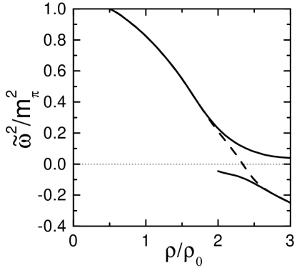
Figure 5: Effective pion gap (75) versus nuclear density, see ref. [9].

where the momentum $\mbox{\boldmath$p$}=\mbox{\boldmath$p$}_{c}$ corresponds to the minimum of the gap at zero mean field $\varphi_{\pi}=0$ [8, 9]. Fig. 5 illustrates the behavior of the effective pion gap $\widetilde{\omega}^{2}({\mbox{\boldmath$p$}}_{c})$ as a function of the baryon density $\rho$. At low densities, $\mbox{Re}\Sigma^{R}_{\pi}$ is small and one obviously has $\widetilde{\omega}^{2}>0$. The dashed line in Fig. 5 describes the case where the $\pi\pi$ fluctuations are artificially switched off and the phase transition turns out to be of second order. At the critical point of the pion condensation ($\rho=\rho_{c}$) this value of $\widetilde{\omega}^{2}$ with switched-off $\pi\pi$ fluctuations changes its sign. In reality the $\pi\pi$ fluctuations are significant in the vicinity of the critical point [64, 65, 66]. The corresponding contribution to the pion self-energy behaves as $T/\widetilde{\omega}(\varphi_{\pi},\mbox{\boldmath$p$}_{c})$ at $T>\mid\widetilde{\omega}^{2}(\varphi_{\pi},\mbox{\boldmath$p$}_{c})/m_{\pi}\mid$, and $\widetilde{\omega}^{2}({\mbox{\boldmath$p$}}_{c})$ does not cross the zero line at all. Rather there are two branches (solid curves in Fig. 5) with positive and respectively negative value for $\widetilde{\omega}^{2}({\mbox{\boldmath$p$}}_{c})$ and the transition becomes of the first order. Calculations of refs [64, 65, 66] demonstrate that at $\rho>\rho_{c}$ the free energy of the state with $\widetilde{\omega}^{2}({\mbox{\boldmath$p$}}_{0})>0$, where the pion mean field is zero, becomes larger than that of the corresponding state with $\widetilde{\omega}^{2}({\mbox{\boldmath$p$}}_{c})<0$ and a finite mean field. Thus, at $\rho=\rho_{c}$ the first-order phase transition to the inhomogeneous pion-condensate state occurs. At $\rho>\rho_{c}$ the state with $\widetilde{\omega}^{2}({\mbox{\boldmath$p$}}_{c})>0$ is meta-stable and the state with $\widetilde{\omega}^{2}({\mbox{\boldmath$p$}}_{c})<0$ and $\widetilde{\varphi}_{\pi}\neq 0$ becomes the ground state.

Before we discuss a self-consistent scheme for a quantitative treatment of this problem we like to qualitatively explain how the instability towards pion condensation develops dynamically. To simplify the treatment we assume that the pion density is low ($\rho_{\pi}\ll\rho$) and further use the fact that the pion is much lighter than the nucleon ($m_{\pi}/m_{N}\simeq 1/7$). This allows us to consider the pion sub-system as a light admixture in a heavy baryon environment, neglecting the feedback of the pions onto the baryons. It provides nucleon Green’s functions unaffected by the pion distribution. This very approximation was used in the first works exploring the possibility of the pion condensation in dense nuclear matter  [5, 6, 7]. We will use it for the pion retarded self-energy, thus neglecting the contribution from pion fluctuations (see dashed curve in Fig. 5). Within the above approximations the quantum kinetic equation (46) for the pion distribution $f_{\pi}$ in homogeneous and equilibrated baryon environment becomes

$$\frac{1}{2}\Gamma B_{\mu}\partial^{\mu}_{X}f_{\pi}=\Gamma_{\mbox{\scriptsize in}}-\Gamma f_{\pi}.$$ (76)

Here $B_{\mu}$ is defined in Eq. (69) and all subscripts $\pi$ are omitted, except for the pion distribution function $f_{\pi}$.

We like now to illustrate that the second branch in Fig. 5 with negative $\widetilde{\omega}^{2}$ constructed under the assumption of vanishing mean field is indeed unstable and becomes stabilized by a finite mean field. The instability of the system can be discussed considering a weak perturbation $\delta f_{\pi}$ of the pion distribution $f^{(0)}_{\pi}=\left[\exp(p_{0}/T)-1\right]^{-1}$ which we assume equilibrated in the rest frame of the system. Linearizing Eq. (76) we find

$$\frac{1}{2}B_{\mu}\partial^{\mu}_{X}\delta f_{\pi}+\delta f_{\pi}=0,$$ (77)

with the solution

$$\delta f_{\pi}(t,p)=\delta f_{0}(p)\exp\left[-2t/B_{0}(p)\right],$$ (78)

where for simplicity the initial fluctuation $\delta f_{0}(p)$ of the pion distribution is assumed to be space-independent. Let us consider the case, where $p_{0}\to 0$ and $\mid\mbox{\boldmath$p$}\mid\simeq p_{F}$. This four-momentum region, being far from the pion mass shell, is right the region, where the pion instability is expected in symmetric nuclear matter. Here the real part of the pion self-energy ${\mathrm{Re}}\Sigma^{R}$ is an even function of the pion energy $p_{0}$ while the width is an odd function and proportional to $p_{0}$ for $p_{0}\rightarrow 0$. Using the results of refs. [8, 9] $2p_{0}-\partial{\mathrm{Re}}\Sigma^{R}/\partial p_{0}\rightarrow 0$, $\Gamma=\beta({\mbox{\boldmath$p$}})p_{0}$ and $\beta({\mbox{\boldmath$p$}})\sim m_{\pi}$ for $p_{0}\rightarrow 0$, we get $B_{0}=\beta({\mbox{\boldmath$p$}})/\widetilde{\omega}^{2}({\mbox{\boldmath$p$}})$ from Eq. (69) and therefore

$$\delta f_{\pi}(t,p_{0}=0,{\mbox{\boldmath$p$}})=\delta f_{0}(p_{0}=0,{\mbox{\boldmath$p$}})\;\exp\left[-2\widetilde{\omega}^{2}({\mbox{\boldmath$p$}})t/\beta({\mbox{\boldmath$p$}})\right].$$ (79)

The above solution shows that for $\widetilde{\omega}^{2}>0$ initial fluctuations are damped, whereas they grow in the opposite case. Thus, the change of sign of $\widetilde{\omega}^{2}(\mbox{\boldmath$p$}_{c})$ leads to an instability of the virtual pion distribution at low energies and momenta $\simeq\mbox{\boldmath$p$}_{c}$. The solution (79) illustrates the important role of the width in the quantum kinetic description. If the width would be neglected in the quantum kinetic equation, one would fail to find the above instability.

The growth of the pion distribution $\delta f_{\pi}$ is accompanied by a growth of the condensate field $\varphi_{\pi}$. Due to the latter the increase of the virtual pion distribution slows down and finally stops when the mean field reaches its stationary value. Therefore, a consistent treatment of the problem requires the solution of the coupled system of the quantum kinetic equation (46) and the mean field equation (50). In order to find the behavior of the virtual pion distribution one also has to include the mean field contribution to the pion self-energy. Considering only small mean fields we keep terms of the lowest-order in $\varphi_{\pi}$. Then $\Sigma^{R}$ acquires an additional contribution $\Sigma^{R}(\varphi_{\pi})=\Sigma^{R}(\varphi_{\pi}=0)+\lambda_{\mbox{\scriptsize eff}}\mid\varphi_{\pi}\mid^{2}$, where $\lambda_{\mbox{\scriptsize eff}}$ denotes the total in-medium pion-pion interaction. Within the same order the mean-field equation becomes

$$\left[\widetilde{\omega}^{2}(\mbox{\boldmath$p$}_{c})+\lambda_{\mbox{\scriptsize eff}}\widetilde{\varphi}_{\pi}^{2}(t)+\frac{1}{2}\beta(\mbox{\boldmath$p$}_{c})\partial_{t}\right]\widetilde{\varphi}_{\pi}(t)=0.$$ (80)

Here we have assumed the simplest structure for the condensate field $\varphi_{\pi}=\widetilde{\varphi}_{\pi}(t)\mbox{exp}({\mathrm{i}}\mbox{\boldmath$p$}_{c}\mbox{\boldmath$r$})$, where $\widetilde{\varphi}_{\pi}(t)$ is a space-homogeneous real function which varies slowly in time. Also one should do the replacement $\widetilde{\omega}^{2}(\mbox{\boldmath$p$}_{c})\rightarrow\widetilde{\omega}^{2}(\varphi_{\pi},\mbox{\boldmath$p$}_{c})\equiv\widetilde{\omega}^{2}(\mbox{\boldmath$p$}_{c})+\lambda_{\mbox{\scriptsize eff}}\mid\varphi_{\pi}\mid^{2}$ in the above equations (76) - (79) for the pion distribution.

The time dependence of $\widetilde{\varphi}$ can qualitatively be understood inspecting the two limits of small and large times. At short times the mean field is still small and one can neglect the $\lambda_{\mbox{\scriptsize eff}}\widetilde{\varphi}^{2}(t)$ term in Eq. (80). Then the mean field

$$\widetilde{\varphi}_{\pi}(t)=\widetilde{\varphi}_{\pi}(0)\exp\left[-2\widetilde{\omega}^{2}(\mbox{\boldmath$p$}_{c})t/\beta(\mbox{\boldmath$p$}_{c}\right]$$ (81)

grows exponentially with time, just like the distribution function (79). Here $\widetilde{\varphi}_{\pi}(0)$ is an initial small fluctuation of the field. At later times the solution of Eq. (80) approaches the stationary limit $\widetilde{\varphi}_{\pi}\rightarrow\widetilde{\varphi}_{\pi}^{\mbox{\scriptsize stat}}$ with

$$(\widetilde{\varphi}_{\pi}^{\mbox{\scriptsize stat}})^{2}=-\widetilde{\omega}^{2}(\mbox{\boldmath$p$}_{c})/\lambda_{\mbox{\scriptsize eff}}(\mbox{\boldmath$p$}_{c}).$$ (82)

Since simultaneously $\widetilde{\omega}^{2}(\varphi_{\pi},\mbox{\boldmath$p$}_{c})=\widetilde{\omega}^{2}(\mbox{\boldmath$p$}_{c})+\lambda_{\mbox{\scriptsize eff}}\mid\varphi_{\pi}\mid^{2}\rightarrow 0$, the change in the pion distribution $\delta f_{\pi}$ will saturate. This stationary solution $\widetilde{\varphi}_{\pi}^{\mbox{\scriptsize stat}}$ is stable as can be seen from linearizing Eq. (80) around $\widetilde{\varphi}_{\pi}^{\mbox{\scriptsize stat}}$

$$\widetilde{\varphi}_{\pi}(t)=\widetilde{\varphi}_{\pi}^{\mbox{\scriptsize stat}}-\delta\widetilde{\varphi}_{0}\exp\left[4\widetilde{\omega}^{2}(\mbox{\boldmath$p$}_{c})t/\beta(\mbox{\boldmath$p$}_{c})\right],$$ (83)

since the exponent is negative. Here $\delta\widetilde{\varphi}_{0}$ denotes an arbitrary initial space-homogeneous fluctuation.

The physics can again be cast into a $\Phi$-derivable form, where the $\Phi$ functional should include at least the following diagrams

$$\Phi = \,\,\parbox{28.45274pt}{ \begin{picture}(10.0,10.0)\immediate\ignorespaces\immediate\ignorespaces\immediate\ignorespaces\immediate\ignorespaces\immediate\ignorespaces\put(0.0,0.0){\includegraphics{migdal-d.18}}\ignorespaces\immediate\ignorespaces\immediate\ignorespaces\immediate\ignorespaces\immediate\ignorespaces\immediate\ignorespaces\immediate\ignorespaces\immediate\ignorespaces\immediate\ignorespaces\immediate\ignorespaces\immediate\ignorespaces\immediate\ignorespaces\immediate\ignorespaces \immediate\ignorespaces{\put(5.0,-2.10876){\makebox(0.0,0.0)[t]{\raisebox{-1.70717pt}{\hskip 28.45274pt(a)}}}}\end{picture}}\,\,+\,\,\parbox{56.9055pt}{ \begin{picture}(20.0,20.0)\immediate\ignorespaces\immediate\ignorespaces\immediate\ignorespaces\immediate\ignorespaces\immediate\ignorespaces\put(0.0,0.0){\includegraphics{migdal-d.19}}\ignorespaces\immediate\ignorespaces\immediate\ignorespaces\immediate\ignorespaces\immediate\ignorespaces\immediate\ignorespaces\immediate\ignorespaces\immediate\ignorespaces\immediate\ignorespaces\immediate\ignorespaces\immediate\ignorespaces\immediate\ignorespaces\immediate\ignorespaces\immediate\ignorespaces\immediate\ignorespaces\immediate\ignorespaces\immediate\ignorespaces \immediate\ignorespaces{\put(17.31732,3.10338){\makebox(0.0,0.0)[lt]{\raisebox{-1.99168pt}{(b)}}}}\end{picture}}\,\,+\,\,\parbox{85.35826pt}{ \begin{picture}(30.0,20.0)\immediate\ignorespaces\immediate\ignorespaces\immediate\ignorespaces\immediate\ignorespaces\immediate\ignorespaces\put(0.0,0.0){\includegraphics{migdal-d.20}}\ignorespaces\immediate\ignorespaces\immediate\ignorespaces\immediate\ignorespaces\immediate\ignorespaces\immediate\ignorespaces\immediate\ignorespaces\immediate\ignorespaces\immediate\ignorespaces\immediate\ignorespaces\immediate\ignorespaces\immediate\ignorespaces\immediate\ignorespaces\immediate\ignorespaces\immediate\ignorespaces\immediate\ignorespaces\immediate\ignorespaces\immediate\ignorespaces\immediate\ignorespaces\immediate\ignorespaces \immediate\ignorespaces{\put(27.9009,3.29892){\makebox(0.0,0.0)[lt]{\raisebox{-1.99168pt}{(c)}}}}\end{picture}}\,\,\dots+\,\,\parbox{85.35826pt}{ \begin{picture}(30.0,20.0)\immediate\ignorespaces\immediate\ignorespaces\immediate\ignorespaces\immediate\ignorespaces\immediate\ignorespaces\put(0.0,0.0){\includegraphics{migdal-d.21}}\ignorespaces\immediate\ignorespaces\immediate\ignorespaces\immediate\ignorespaces\immediate\ignorespaces\immediate\ignorespaces\immediate\ignorespaces\immediate\ignorespaces\immediate\ignorespaces\immediate\ignorespaces\immediate\ignorespaces\immediate\ignorespaces\immediate\ignorespaces\immediate\ignorespaces\immediate\ignorespaces\immediate\ignorespaces\immediate\ignorespaces\immediate\ignorespaces\immediate\ignorespaces \immediate\ignorespaces{\put(27.9009,3.29892){\makebox(0.0,0.0)[lt]{\raisebox{-1.99168pt}{(d)}}}\put(12.00027,2.00012){\makebox(0.0,0.0)[l]{{$\dots$}}}}\end{picture}}$$

$$+ \,\,\parbox{31.29802pt}{ \immediate\ignorespaces\immediate\ignorespaces\immediate\ignorespaces\immediate\ignorespaces\immediate\ignorespaces\leavevmode\includegraphics{migdal-d.22}\ignorespaces\immediate\ignorespaces\immediate\ignorespaces\immediate\ignorespaces\immediate\ignorespaces\immediate\ignorespaces\immediate\ignorespaces\immediate\ignorespaces\immediate\ignorespaces\immediate\ignorespaces\immediate\ignorespaces\immediate\ignorespaces\immediate\ignorespaces\immediate\ignorespaces\immediate\ignorespaces \immediate\ignorespaces}_{\mbox{(e)}}+\,\,\parbox{31.29802pt}{ \immediate\ignorespaces\immediate\ignorespaces\immediate\ignorespaces\immediate\ignorespaces\immediate\ignorespaces\leavevmode\includegraphics{migdal-d.23}\ignorespaces\immediate\ignorespaces\immediate\ignorespaces\immediate\ignorespaces\immediate\ignorespaces\immediate\ignorespaces\immediate\ignorespaces\immediate\ignorespaces\immediate\ignorespaces\immediate\ignorespaces\immediate\ignorespaces\immediate\ignorespaces\immediate\ignorespaces\immediate\ignorespaces\immediate\ignorespaces \immediate\ignorespaces}_{\mbox{(f)}}+\;\;\parbox{48.36967pt}{ \immediate\ignorespaces\immediate\ignorespaces\immediate\ignorespaces\immediate\ignorespaces\immediate\ignorespaces\leavevmode\includegraphics{migdal-d.24}\ignorespaces\immediate\ignorespaces\immediate\ignorespaces\immediate\ignorespaces\immediate\ignorespaces\immediate\ignorespaces\immediate\ignorespaces\immediate\ignorespaces\immediate\ignorespaces\immediate\ignorespaces\immediate\ignorespaces \immediate\ignorespaces}_{\raisebox{-8.53581pt}{\mbox{(g)}}}+\,\,\parbox{36.98857pt}{ \immediate\ignorespaces\immediate\ignorespaces\immediate\ignorespaces\immediate\ignorespaces\immediate\ignorespaces\leavevmode\includegraphics{migdal-d.25}\ignorespaces\immediate\ignorespaces\immediate\ignorespaces\immediate\ignorespaces\immediate\ignorespaces\immediate\ignorespaces\immediate\ignorespaces\immediate\ignorespaces\immediate\ignorespaces\immediate\ignorespaces\immediate\ignorespaces\immediate\ignorespaces\immediate\ignorespaces \immediate\ignorespaces}_{\raisebox{-14.22636pt}{\mbox{(h)}}}+\,\,\parbox{36.98857pt}{ \immediate\ignorespaces\immediate\ignorespaces\immediate\ignorespaces\immediate\ignorespaces\immediate\ignorespaces\leavevmode\includegraphics{migdal-d.26}\ignorespaces\immediate\ignorespaces\immediate\ignorespaces\immediate\ignorespaces\immediate\ignorespaces\immediate\ignorespaces\immediate\ignorespaces\immediate\ignorespaces\immediate\ignorespaces\immediate\ignorespaces\immediate\ignorespaces\immediate\ignorespaces\immediate\ignorespaces\immediate\ignorespaces \immediate\ignorespaces}_{\raisebox{-14.22636pt}{\mbox{(i)}}}$$ (84)

Here bold and bold-wavy lines relate to baryon and pion Green’s functions, respectively, while the wavy line terminated by cross denotes the pion condensate. Since in the broken phase the mean pion field mixes nucleon with $\Delta$ configurations we adopt the $SU(4)$ formulation of the model, introduced in ref. [67]. There one deals with a unified description of baryons ($N$ and $\Delta$), based on $20\times 20$ matrix Hamiltonian in the basis of $20$ $\Delta$–nucleon spin–isospin states. Thus, the solid lines symbolize a unified propagator matrix for $\Delta$-resonance and nucleon. The mixing is provided by condensate–baryon coupling (diagram (g)). Numerical symmetry factors are omitted in Eq. (8).

Functional variation of $\Phi$ with respect to propagators provides the corresponding self-energies. Diagrammatically this variation corresponds to cutting and opening the respective propagator lines of the diagrams of $\Phi$ in Eq. (8). Thus diagrams (a) to (d), (f) and (h) contribute to the pion self-energy. Diagram (a) accounts for the baryon particle–hole contributions to the pion self-energy. It includes $NN^{-1}$, $\Delta N^{-1}$, $N\Delta^{-1}$ and $\Delta\Delta^{-1}$ terms. The subsequent series of diagrams (b) to (d) renormalizes baryon–pion vertex including baryon–baryon correlations in terms of the Landau–Migdal parameter $g^{\prime}$. Diagram (f) accounts for the pion fluctuations. It is proportional to $\sim{T}/{\widetilde{\omega}(\varphi_{\pi},\mbox{\boldmath$p$}_{c})}$ and thus causes the transition to be of first order. This becomes especially important for the case of heated and even non-equilibrium dense matter, where the effective pion gap [65, 66] drops. One should notice that pion fluctuation contributions are also present in the particle-hole diagram (a) when opened perturbatively. Diagram (h) corresponds to pion interactions with the condensate which is responsible for the stabilization of the condensate solution (82).

Likewise cutting and opening the solid lines in $\Phi$ determines the baryon self-energy which describes the feedback of the pions onto the baryonic subsystem. This feedback is required for the conserving and thermodynamically consistent treatment of the problem. Diagrams of the first line correspond to the modification of the baryon motion by the multiple interaction with the pions corrected by correlations. Diagram (e) generates a purely local interaction contribution whereas diagram (g) with the coupling of the condensate to baryons leads to the mixing of $N$ and $\Delta$.

Variation of $\Phi$ with respect to the condensates (wavy line with cross) determines the source term $J$ in the equation for the mean field (50). The value $\lambda_{\mbox{\scriptsize eff}}$ entering Eq. (80) is generated by the the last two diagrams (h) and (i) of Eq. (8).

The kinetic description (46) for the particle distribution together with the equation of motion for the mean field (50) is still insufficient for the numerical simulations of the dynamics of the phase transition. The reason is that the creation of seeds of the new phase, which initiate the growth of the mean field and the particle distribution, is due to fluctuations, cf. Eqs. (79) and (81). However, the scheme of Eqs. (46) and (50) provides no sources of stochastic fluctuations. Thus, it can only simulate the dynamics of one of the phases rather than the transition between them. The required stochastic sources may be introduced into the transport theory in the spirit of the Boltzmann–Langevin approach developed in refs [68, 69, 70] and the stochastic interpretation of the Kadanoff–Baym equations [71]. The stochastic transport approach offers an appropriate framework for the description of the unstable dynamics by means of a stochastic force in the mean field equation and a stochastic collision term in the transport equation, which both act as a source for a continuous branching of the dynamical trajectories.

The above example shows that we really need the off-mass-shell kinetics to describe the dynamics of the pion-condensate phase transition, since the corresponding instability of the pion distribution function occurs far from the pion mass shell, cf. Eq. (79). Besides the conserving property and thermodynamic consistency of the $\Phi$-derivable approximation it also leads us to the proper order of the phase transition.

9 Summary and Prospects

A number of problems arising in different dynamical systems, e.g. in heavy-ion collisions, require an explicit treatment of dynamical evolution of particles with finite mass-width. This was demonstrated for the example of bremsstrahlung from a nuclear source, where the soft part of the spectrum can be reproduced only provided the mass-widths of nucleons in the source are taken explicitly into account. In this case the mass-width arises due to collisional broadening of nucleons. Another examples considered concern propagation of broad resonances (like $\rho$-meson and $\Delta$) in the medium. Decays of $\rho$-mesons are an important source of di-leptons radiated by excited nuclear matter. As shown, a consistent description of the invariant-mass spectrum of radiated di-leptons can be only achieved if one accounts for the in-medium modification of the $\rho$-meson width (more precisely, its spectral function). The principle of actio = re-actio was demonstrated on a pedagogical example when there is only $\pi N\Delta$ coupling and in the limit of a dilute nuclear matter. We also expect a consistent description of chiral $\sigma$-, $\pi$- condensates together with fluctuations, as an immediate application of our results to multi-component systems.

We have argued that the Kadanoff–Baym equation within the first-order gradient approximation, slightly modified to make the set of Dyson’s equations exactly consistent (rather than up to the second-order gradient terms), together with algebraic equation for the spectral function provide a proper frame for a quantum four-phase-space kinetic description that applies also to systems of unstable particles. The quantum four-momentum-space kinetic equation proves to be charge and energy–momentum conserving and thermodynamically consistent, provided it is based on a $\Phi$-derivable approximation. The $\Phi$ functional also gives rise to a very natural representation of the collision term. Various self-consistent approximations are known since long time which do not explicitly use the $\Phi$-derivable concept like self-consistent Born and T-matrix approximations. The advantage the $\Phi$ functional method consists in offering a regular way of constructing various self-consistent approximations.

We have also addressed the question whether a closed non-equilibrium system approaches the thermodynamic equilibrium during its evolution. We obtained a definite expression for a local (Markovian) entropy flow and were able to explicitly demonstrate the $H$-theorem for some of the common choices of $\Phi$ approximations. This expression holds beyond the quasiparticle picture and thus generalizes the well-known Boltzmann kinetic entropy. Memory effects in the quantum four-momentum-space kinetics were discussed and a general strategy to deduce memory corrections to the entropy was outlined.

At the example of pion-condensate phase transition in symmetric nuclear matter we demonstrated important role of the width effects in the dynamics and we formulated a self-consistent $\Phi$ derivable scheme for the transport treatment of this problem. An interesting application of such self-consistent transport description is possible to dynamics of the phase transition of a neutron star to the pion or kaon condensate state accompanied by the corresponding neutrino burst. In view of the letter, another application concerns description of the neutrino transport in supernovas and hot neutron stars during first few minutes of their evolution. At an initial stage, neutrinos typically of thermal energy, produced outside (in the mantel) and inside the neutron-star core, are trapped within the regions of production. However, coherent effects in neutrino production and their rescattering on nucleons [23] reduce the opacity of the nuclear-medium and may allow for soft neutrinos to escape the core and contribute to the heating off the mantle. The extra energy transport may be sufficient to blow off the supernova’s mantle in the framework of the shock-reheating mechanism [72]. The description of the neutrino transport in the semi-transparent region should therefore be treated with the due account of mass-widths effects.

Further applications concern relativistic plasmas, such as QCD and QED plasmas. The plasma of deconfined quarks and gluons was present in the early Universe, it may exist in cores of massive neutron stars, and may also be produced in laboratory in ultra-relativistic nucleus–nucleus collisions. All these systems need a proper treatment of particle transport. Perturbative description of soft-quanta propagation suffers of infrared divergences and one needs a systematic study of the particle mass-width effects in order to treat them, cf. ref. [23]. A thermodynamic $\Phi$-derivable approximation for hot relativistic QED plasmas—a gas of electrons and positrons in a thermal bath of photons—was recently considered in ref.  [73]. Their treatment may be also applied to the high-temperature super-conductors and the fractional quantum Hall effect [74, 75]. Formulated above approach allows for a natural generalization of such a $\Phi$-derivable schemes to the dynamical case.

Acknowledgment: We are grateful to G. Baym, G.E. Brown, P. Danielewicz, H. Feldmeier, B. Friman, C. Greiner, E.E. Kolomeitsev, P.C. Martin, U. Mosel and S. Leupold for fruitful discussions. Two of us (Y.B.I. and D.N.V.) highly appreciate the hospitality and support rendered to us at Gesellschaft für Schwerionenforschung. This work has been supported in part by DFG (project 436 Rus 113/558/0). Y.B.I and D.N.V. were partially supported by RFBR grant NNIO-00-02-04012. Y.B.I. was also partially supported by RFBR grant 00-15-96590.

References

- [1] L.D. Landau, ZhETF 30, 1058 (1956) [ Sov. Phys. JETP 3, 920 (1956)].
- [2] A.B. Migdal, Nuclear Theory: the Quasiparticle Method, W.A. Benjamin, N.Y. 1968.
- [3] A.B. Migdal, Theory of Finite Fermi Systems and properties of Atomic Nuclei, Wiley and Sons, New York 1967 (Russ. ed. 1965), 2-nd edition, Moscow, Nauka 1983 in Russian.
- [4] E.M. Lifshiz and L.P. Pitaevskii, Statistical Physics P2, V9, Pergamon 1980.
- [5] A.B. Migdal, ZhETF 61, 2209 (1971) [Sov. Phys. JETP 34, 1184 (1972)].
- [6] A.B. Migdal, ZhETF 63, 1993 (1972) [Sov. Phys. JETP 36, 1052 (1973)].
- [7] A.B. Migdal, Phys. Rev. Lett. 31, 257 (1973); Nucl. Phys. A210, 421 (1973); Phys. Lett. 47B, 96 (1973), 52B, 172, 264 (1974).
- [8] A.B. Migdal, Rev. Mod. Phys. 50, 107 (1978).
- [9] A. B. Migdal, E. E. Saperstein, M. A. Troitsky and D.N.Voskresensky, Phys. Rep. 192, 179 (1990).
- [10] D.N. Voskresensky, Nucl. Phys. A555, 293 (1993).
- [11] L. D. Landau and I. Pomeranchuk, Dokl. Akad. Nauk SSSR 92, 553, 735 (1953); also in ”Collected Papers of Landau”, ed. Ter Haar (Gordon & Breach, 1965) papers 75 - 77.
- [12] A. B. Migdal, Phys. Rev. 103, 1811 (1956) [ Sov. Phys. JETP 5, 527 (1957)].
- [13] P. L. Anthony, et al., Phys. Rev. Lett. 75, 1949 (1995); S. Klein, Rev. Mod. Phys. 71, 1501 (1999).
- [14] J. Schwinger, J. Math. Phys. 2, 407 (1961).
- [15] L.P. Kadanoff and G. Baym, Quantum Statistical Mechanics (Benjamin, 1962).
- [16] L.P. Keldysh, ZhETF 47, 1515 (1964) [Sov. Phys. JETP 20, 1018 (1965)].
- [17] G. Baym and L.P. Kadanoff, Phys. Rev. 124, 287 (1961).
- [18] G. Baym, Phys. Rev. 127, 1391 (1962).
- [19] J. M. Luttinger and J. C. Ward, Phys. Rev. 118, 1417 (1960).
- [20] A.A. Abrikosov, L.P. Gorkov, I.E. Dzyaloshinski, Methods of Quantum Field Theory in Statistical Physics , Dover Pub., INC. N.Y., 1975.
- [21] Yu.B. Ivanov, J. Knoll, and D.N. Voskresensky, Nucl. Phys. A 657, 413 (1999).
- [22] Yu.B. Ivanov, J. Knoll and D.N. Voskresensky, Nucl. Phys. A 672, 313 (2000).
- [23] J. Knoll and D.N. Voskresensky, Ann. Phys. 249, 532 (1996); Phys. Lett. B 351, 43 (1995).
- [24] H. van Hees and J. Knoll, proceedings of the Intern. Workshop XXVIII on Gross Properties of Nuclei and Nuclear Excitations, Hirschegg, Austria, Jan 16-22,2000, hep-ph/0002087, and to be published.
- [25] W. Weinhold, B.L. Friman, and W. Nörenberg, Acta Phys. Pol. 27, 3249 (1996); Phys. Lett. B 433, 236 (1998).
- [26] J. Knoll and C. Guet, Nucl. Phys. A 494, 334 (1989); M. Durand and J. Knoll, Nucl. Phys. A 496, 539 (1989).
- [27] D. N. Voskresensky and A. V. Senatorov, Yad. Fiz. 45, 657 (1987) [in Engl. translation Sov.J.Nucl.Phys. 45, 411 (1987).
- [28] J. Knoll, proceedings of the Erice School on Nuclear Physics in Erice, Sicily, Italy, September 17 -25 1998, published in Progress in Particle and Nuclear Physics 42, 177 (1999).
- [29] M. Herrmann, B.L. Friman, and W. Nörenberg, Nucl. Phys. A 560, 411 (1993).
- [30] R. Rapp, G. Chanfray, and J. Wambach, Nucl. Phys. A 617, 472 (1997).
- [31] S. Leupold, U. Mosel, Phys. Rev. C 58, 2939 (1998).
- [32] F. Klingl, N. Kaiser, and W. Weise, Nucl. Phys. A 624, 527 (1997).
- [33] B.L. Friman and H.-J. Pirner, Nucl. Phys. A 617, 496 (1997)
- [34] B. Friman, M. Lutz and G. Wolf, nucl-th/9811040, in Proc. ”Baryons 98”, Bonn, 22.-26. September 1998, World Scientific 1999, 663-674 and in Proc. ”Intern. Workshop XXVII on Gross Properties of Nuclei and Nuclear Excitations”, Hirschegg, January 2000; nucl-th/0003012.
- [35] P. Danielewicz and G.F. Bertsch, Nucl. Phys. A 533, 712 (1991).
- [36] M. Effenberger, E.L. Bratkovskaya and U. Mosel, Phys. Rev. C 60, 051901 (1999).
- [37] M. Effenberger, E.L. Bratkovskaya, W. Cassing, U. Mosel, Phys. Rev. C 60 027601 (1999).
- [38] E. Beth, G.E. Uhlenbeck, Physica 4, 915 (1937).
- [39] K. Huang, ”Statistical Mechanics”, Wiley, New York (1963).
- [40] R. Dashen, S. Ma, H.J. Bernstein, Phys.Rev. 187, 345 (1969).
- [41] A. Z. Mekjian, Phys. Rev. C 17, 1051 (1978).
- [42] R. Venugopalan and M. Prakash, Nucl. Phys. A 456, 718 (1992).
- [43] W. Lenz, Z. Phys. 56, 778 (1929).
- [44] L.D. Landau and E.M. Lifshiz, Quantum Mechanics, Part 3, Pergamon press, 1977.
- [45] C.B. Dover, J. Hüfner and R.H. Lemmer, Ann. Phys. (NY) 66, 248 (1971).
- [46] M. Lutz, A. Steiner and W. Weise, Nucl. Phys. A 574, 755 (1994).
- [47] P. Danielewicz and S. Pratt, Phys.Rev. C53, 249 (1996).
- [48] W. Botermans and R. Malfliet, Phys. Rep. 198, 115 (1990).
- [49] S. Leupold, Nucl. Phys. A 672, 475 (2000).
- [50] W. Cassing and S. Juchem, Nucl.Phys.A 672, 417 (2000).
- [51] B. Bezzerides and D.F. DuBois, Ann. Phys. (N.Y.) 70, 10 (1972).
- [52] P. Lipavsky, V. Spicka and B. Velicky, Phys. Rev. D 34, 6933 (1986).
- [53] V. Spicka and P. Lipavsky, Phys. Rev. Lett. 73, 3439 (1994); Phys. Rev. B 52, 14615 (1995).
- [54] W.D. Kraeft, D. Kremp, W. Ebeling and G. Röpke, Quantum Statistics of Charged Particle Systems (Akademie-Verlag, Berlin, 1986).
- [55] M. Bonitz, Quantum Kinetic Theory (Teubner, Stuttgart/Leipzig, 1998).
- [56] Th. Bornath, D. Kremp, W. D. Kraeft, and M. Schlanges, Phys. Rev. E 54, 3274 (1996).
- [57] M. Schönhofen, M. Cubero, B. Friman, W. Nörenberg and Gy. Wolf, Nucl. Phys. A 572, 112 (1994).
- [58] S. Jeon and L.G. Yaffe, Phys. Rev. D 53, 5799 (1996).
- [59] D.N. Voskresensky, D. Blaschke, G. Röpke and H. Schulz, Int. Mod. Phys. J. E 4, 1 (1995).
- [60] J.M. Cornwall, R. Jackiw and E. Tomboulis, Phys. Rev. D 10, 2428 (1974).
- [61] G. Baym and C. Pethick, Landau Fermi–Liquid Theory (John Wiley and Sons, INC, N.Y., 1991).
- [62] G.M. Carneiro and C. J. Pethick, Phys. Rev. B 11, 1106 (1975).
- [63] Akmal, A., Pandharipande, V. R., and Ravenhall, D. G., Phys. Rev.C 58, 1804 (1998).
- [64] A.M. Dyugaev,Pisma v ZhETF 22, 181 (1975).
- [65] D.N. Voskresensky and I.N. Mishustin, Pisma v ZhETF 34, 317 ( 1981) [in Engl.: JETP Lett. 34, 303 (1981)]; Yad. Fiz. 35, ( 1982) [in Engl.:Sov. J. Nucl. Phys. 35, 667 (1982)].
- [66] A.M. Dyugaev, Pisma v ZhETF. 35, 341 (1982); ZhETF 83, 1005 (1982); Yad. Fiz. 38, 1131 (1983) [in Engl.:Sov. J. Nucl. Phys. 38, 680 (1983)].
- [67] D. Campbell, R. Dashen and J. Manassash, Phys. Rev. D12, 979, 1010 (1975).
- [68] S. Ayik and C. Gregoire, Phys. Lett. B212, 269 (1988); Nucl. Phys. A513, 187 (1990).
- [69] J. Randrup and B. Remaud, Nucl. Phys. A514, 339 (1990).
- [70] Yu.B. Ivanov and S. Ayik, Nucl.Phys. A593, 233 (1995).
- [71] C. Greiner and S. Leupold, Ann. Phys. 270, 328 (1998).
- [72] H.A. Bethe and J.R. Wilson, Astroph. J. 295, 14 (1985).
- [73] B. Vanderheyden and G. Baym, J. Stat. Phys. 93, 843 (1998).
- [74] B.I. Halperin, P.A. Lee and N. Read, Phys Rev. B47, 7312 (1993).
- [75] L.B. Ioffe and A.I. Larkin, B39, 8988 (1989).