ANL-PHY-9530-TH-2000

nucl-th/0005064

DYSON-SCHWINGER EQUATIONS:

DENSITY, TEMPERATURE AND CONTINUUM STRONG QCD

Craig D. Roberts and Sebastian M. Schmidt

Physics Division, Building 203, Argonne National Laboratory, Argonne, IL 60439-4843, USA

e-mail: cdroberts@anl.gov     basti@theory.phy.anl.gov

ABSTRACT
Continuum strong QCD is the application of models and continuum quantum field theory to the study of phenomena in hadronic physics, which includes; e.g., the spectrum of QCD bound states and their interactions; and the transition to, and properties of, a quark gluon plasma. We provide a contemporary perspective, couched primarily in terms of the Dyson-Schwinger equations but also making comparisons with other approaches and models. Our discourse provides a practitioners’ guide to features of the Dyson-Schwinger equations [such as confinement and dynamical chiral symmetry breaking] and canvasses phenomenological applications to light meson and baryon properties in cold, sparse QCD. These provide the foundation for an extension to hot, dense QCD, which is probed via the introduction of the intensive thermodynamic variables: chemical potential and temperature. We describe order parameters whose evolution signals deconfinement and chiral symmetry restoration, and chronicle their use in demarcating the quark gluon plasma phase boundary and characterising the plasma’s properties. Hadron traits change in an equilibrated plasma. We exemplify this and discuss putative signals of the effects. Finally, since plasma formation is not an equilibrium process, we discuss recent developments in kinetic theory and its application to describing the evolution from a relativistic heavy ion collision to an equilibrated quark gluon plasma.

PACS:              05.20.Dd, 11.10.Wx, 11.15.Tk, 12.38.Mh, 24.85.+p, 25.75.Dw

KEYWORDS:

Dyson-Schwinger Equations, Hadron Physics, Kinetic Theory, Nonperturbative QCD Modelling, Particle Production, Quark-Gluon Plasma

To appear in:
Progress in Particle and Nuclear Physics 45 (2000) 2nd issue

1 Prologue

Continuum strong QCD. The phrase comes to us via Ref. [1], although that is likely not its debut. In our usage it embraces all continuum nonperturbative methods and models that seek to provide an intuitive understanding of strong interaction phenomena, and particularly those where a direct connection with QCD can be established, in one true limit or another. The community of continuum strong QCD practitioners is a large one and that is helped by the appealing simplicity of models, which facilitates insightful contributions that are not labour intensive.

Our goal is to present an image of the gamut of strong QCD phenomena currently at the forefront of the interaction between experiment and theory, and of contemporary methods and their application. Our portrayal will not be complete but ought to serve as a conduit into this field. We judge that the best means to pursue our aim is to focus on a particular approach, making connections and comparisons with others when possible and helpful. All methods have strengths and weaknesses, and, when modelling is involved, they are not always obviously systematic. That is the cost of leaving perturbation theory behind. They can also yield internally consistent results that nevertheless are without fidelity to QCD. Vigilance is therefore necessary but herein lies another benefit of a leagued community.

Everyone has a favourite tool and the Dyson-Schwinger equations [DSEs] are ours: they provide the primary medium for this discourse. The framework is appropriate here because the last decade has seen something of a renaissance in its phenomenological application and we chronicle that herein. Additionally, the DSEs have been applied simultaneously to phenomena as apparently unconnected as low-energy $\pi\pi$ scattering, $B\to D^{\ast}$ decays and the equation of state for a quark gluon plasma, and hence they provide a single framework that serves to conduct us through a wide range of hadron physics. Focusing on one approach is no impediment to a broad perspective: the continuum, nonperturbative studies complement each other, with agreement between them being a strong signal of a real effect. In this and their flexibility they provide a foil to the phlegmatic progress of numerical simulations of lattice-QCD, and a fleet guide to unanticipated phenomena.

To close this short introduction we present a list of abbreviations. They are defined in the text when first introduced, however, that point can be difficult to locate.

BSA	…	Bethe-Salpeter amplitude	BSE	…	Bethe-Salpeter equation
DCSB	…	dynamical chiral symmetry breaking	DSE	…	Dyson-Schwinger equation
EOS	…	equation of state	LHC	…	large hadron collider
QCD	…	quantum chromodynamics	QC2D	…	two-colour QCD
QED	…	quantum electrodynamics	QED3	…	three-dimensional QED
QGP	…	quark gluon plasma	RHIC	…	relativistic heavy ion collider

2 Dyson-Schwinger Equations

In introducing the DSEs we find useful the brief text book discussions in Chap. 10 of Ref. [2] and Chap. 2 of Ref. [3], and particularly their use in proving the renormalisability of quantum electrodynamics [QED] in Ref. [4], Chap. 19. However, these sources do not cover the use of DSEs in contemporary nuclear and high-energy physics. Reference [5] ameliorates that with a wide ranging review of the theoretical and phenomenological applications extant when written, and it provides a good foundation for us.

The DSEs are a nonperturbative means of analysing a quantum field theory. Derived from a theory’s Euclidean space generating functional, they are an enumerable infinity of coupled integral equations whose solutions are the $n$-point Schwinger functions [Euclidean Green functions], which are the same matrix elements estimated in numerical simulations of lattice-QCD. In theories with elementary fermions, the simplest of the DSEs is the gap equation, which is basic to studying dynamical symmetry breaking in systems as disparate as ferromagnets, superconductors and QCD. The gap equation is a good example because it is familiar and has all the properties that characterise each DSE: its solution is a $2$-point function [the fermion propagator] while its kernel involves higher $n$-point functions; e.g., in a gauge theory, the kernel is constructed from the gauge-boson $2$-point function and fermion–gauge-boson vertex, a $3$-point function; a weak-coupling expansion yields all the diagrams of perturbation theory; and solved self-consistently, the solution of the gap equation exhibits nonperturbative effects unobtainable at any finite order in perturbation theory; e.g, dynamical symmetry breaking.

The coupling between equations; i.e., the fact that the equation for a given $m$-point function always involves at least one $n>m$-point function, necessitates a truncation of the tower of DSEs in order to define a tractable problem. One systematic and familiar truncation is a weak coupling expansion to reproduce perturbation theory. However, that precludes the study of nonperturbative phenomena and hence something else is needed for the investigation of strongly interacting systems, bound state phenomena and phase transitions.

In analysing the ferromagnetic transition, the Hartree-Fock approximation yields qualitatively reliable information and in QED and QCD its analogue: the rainbow truncation, has proven efficacious. However, a priori it can be difficult to judge whether a given truncation will yield reliable results and a systematic improvement is not always obvious. It is here that some model-dependence enters but that is not new, being typical in the study of strongly-interacting few- and many-body systems. To proceed with the DSEs one just employs a truncation and explores its consequences, applying it to different systems and constraining it, where possible, by comparisons with experimental data and other theoretical approaches on their common domain. In this way a reliable truncation can be identified and then attention paid to understanding the keystone of its success and improving its foundation. This pragmatic approach has proven rewarding in strong QCD, as we shall describe.

2.1 DSE Primer

Lattice-QCD is defined in Euclidean space because the zero chemical potential [$\mu=0$] Euclidean QCD action defines a probability measure, for which many numerical simulation algorithms are available. The Gaussian distribution:

$${\cal K}_{t}(q,q^{\prime})=(2\pi t)^{-3/2}\,\exp[-\left(q-q^{\prime}\right)^{2}/(2t)]\,,$$ (2.1.1)

defines the simplest probability measure: $dq^{\prime}\,{\cal K}_{t}(q,q^{\prime})$. ${\cal K}_{t}$ is positive and normalisable, which allows its interpretation as a probability density. An heuristic exposition of probability measures in quantum field theory can be found in Ref. [3], Chap. 6, while Ref. [6], Chaps. 3 and 6, provides a more rigorous discussion in the context of quantum mechanics and quantum field theory.

Working in Euclidean space, however, is more than simply pragmatic: Euclidean lattice field theory is currently a primary candidate for the rigorous definition of an interacting quantum field theory [6, 7] and that relies on it being possible to define the generating functional via a proper limiting procedure. The moments of the measure; i.e., vacuum expectation values of the fields, are the $n$-point Schwinger functions and the quantum field theory is completely determined once all its Schwinger functions are known. The time-ordered Green functions of the associated Minkowski space theory can be obtained in a well-defined fashion from the Schwinger functions. This is one reason why we employ a Euclidean formulation. Another is a desire to maintain contact with perturbation theory where the renormalisation group equations for QCD and their solutions are best understood [8].

To make clear our conventions: for $4$-vectors $a$, $b$:

$$a\cdot b:=a_{\mu}\,b_{\nu}\,\delta_{\mu\nu}:=\sum_{i=1}^{4}\,a_{i}\,b_{i}\,,$$ (2.1.2)

so that a spacelike vector, $Q_{\mu}$, has $Q^{2}>0$; our Dirac matrices are Hermitian and defined by the algebra

$$\{\gamma_{\mu},\gamma_{\nu}\}=2\,\delta_{\mu\nu}\,;$$ (2.1.3)

and we use

$$\gamma_{5}:=-\,\gamma_{1}\gamma_{2}\gamma_{3}\gamma_{4}$$ (2.1.4)

so that

$${\rm tr}\left[\gamma_{5}\gamma_{\mu}\gamma_{\nu}\gamma_{\rho}\gamma_{\sigma}\right]=-4\,\varepsilon_{\mu\nu\rho\sigma}\,,\;\varepsilon_{1234}=1\,.$$ (2.1.5)

The Dirac-like representation of these matrices is:

$$\vec{\gamma}=\left(\begin{array}[]{cc}0&-i\vec{\tau}\\ i\vec{\tau}&0\end{array}\right),\;\gamma_{4}=\left(\begin{array}[]{cc}\tau^{0}&0\\ 0&-\tau^{0}\end{array}\right),$$ (2.1.6)

where the $2\times 2$ Pauli matrices are:

$$\tau^{0}=\left(\begin{array}[]{cc}1&0\\ 0&1\end{array}\right),\;\tau^{1}=\left(\begin{array}[]{cc}0&1\\ 1&0\end{array}\right),\;\tau^{2}=\left(\begin{array}[]{cc}0&-i\\ i&0\end{array}\right),\;\tau^{3}=\left(\begin{array}[]{cc}1&0\\ 0&-1\end{array}\right).$$ (2.1.7)

Using these conventions the [unrenormalised] Euclidean QCD action is

$$S[\bar{q},q,A]=\ \int d^{4}x\,\left[\mbox{\footnotesize$\frac{1}{4}$}\,F_{\mu\nu}^{a}F_{\mu\nu}^{a}+\mbox{\footnotesize$\frac{1}{2\xi}$}\,\partial\cdot A^{a}\,\partial\cdot A^{a}+\sum_{f=1}^{N_{f}}\,\bar{q}_{f}\left(\gamma\cdot\partial+m_{f}+ig\,\mbox{\footnotesize$\frac{1}{2}$}\lambda^{a}\,\gamma\cdot A^{a}\right)q_{f}\right],$$ (2.1.8)

where: $F_{\mu\nu}^{a}=\partial_{\mu}A_{\nu}^{a}-\partial_{\nu}A_{\mu}^{a}-gf^{abc}A_{\mu}^{b}A_{\nu}^{s}$; $N_{f}$ is the number of quark flavours; $m_{f}$ are the current-quark masses; $\{\lambda^{a}:a=1,\ldots,8\}$ with $[\lambda^{a},\lambda^{b}]=2if^{abc}\lambda^{c}$ are the Gell-Mann matrices for $SU(3)$ colour; and $\xi$ is the covariant gauge fixing parameter. The generating functional follows:

$${\cal Z}[\bar{\eta},\eta,J]=\int\,d\mu(\bar{q},q,A,\bar{\omega},\omega)\,\exp\int d^{4}x\left[\bar{q}\,\eta+\bar{\eta}\,q+J_{\mu}^{a}\,A_{\mu}^{a}\right],$$ (2.1.9)

with sources: $\bar{\eta}$, $\eta$, $J$, and a functional integral measure

$$d\mu(\bar{q},q,A,\bar{\omega},\omega):=$$

$$\prod_{x}\prod_{\phi}{\cal D}\bar{q}_{\phi}(x){\cal D}q_{\phi}(x)\prod_{a}{\cal D}\bar{\omega}^{a}(x){\cal D}\omega^{a}(x)\prod_{\mu}{\cal D}A_{\mu}^{a}(x)\exp(-S[\bar{q},q,A]-S^{g}[\bar{\omega},\omega,A])\,,$$

where $\phi$ represents both the flavour and colour index of the quark field, and $\bar{\omega}$ and $\omega$ are scalar, Grassmann [ghost] fields that are a necessary addition in covariant gauges, and most other gauges too. [Without gauge fixing the action is constant along trajectories of gauge-equivalent gluon field configurations, which leads to a gauge-orbit volume-divergence in the continuum generating functional.] The normalisation

$${\cal Z}[\bar{\eta}=0,\eta=0,J=0]=1$$ (2.1.11)

is implicit in the measure.

The ghosts only couple directly to the gauge field:

$$S_{g}[\bar{\omega},\omega,A]=\int d^{4}x\,\left[-\partial_{\mu}\bar{\omega}^{a}\,\partial_{\mu}\omega^{a}-gf^{abc}\,\partial_{\mu}\bar{\omega}^{a}\,\omega^{b}\,A_{\mu}^{c}\right]\,,$$ (2.1.12)

and restore unitarity in the subspace of transverse [physical] gauge fields. Practically, the normalisation means that ghost fields are unnecessary in the calculation of gauge invariant observables using lattice-regularised QCD because the gauge-orbit volume-divergence in the generating functional, associated with the uncountable infinity of gauge-equivalent gluon field configurations in the continuum, is rendered finite by the simple expedient of only summing over a finite number of configurations.

It is not necessary to employ the covariant gauge fixing condition in constructing the measure although it does yield DSEs with a simple form. Indeed a rigorous definition of the measure may require a gauge fixing functional that either completely eliminates Gribov copies or restricts the functional integration domain to a subspace without them. Concerned, as they are, with unobservable degrees of freedom, such modifications of the measure cannot directly affect the colour-singlet $n$-point functions that describe physical observables. However, they have the capacity to modify the infrared behaviour of coloured $n$-point functions [9, 10] and thereby influence the manner in which we intuitively understand observable effects.

The DSEs are derived from the generating functional using the elementary observation that, with sensible Euclidean space boundary conditions, the integral of a total derivative is zero:

$$0=\int\,\frac{\delta}{\delta A}\,d\mu(\bar{q},q,A,\bar{\omega},\omega)\,\exp\int d^{4}x\left[\bar{q}\,\eta+\bar{\eta}\,q+J_{\mu}^{a}\,A_{\mu}^{a}\right].$$ (2.1.13)

Examples of such derivations: the QED gap equation, the equation for the photon vacuum polarisation and that for the fermion-fermion scattering matrix [a $4$-point function], are presented in Ref. [2], Chap. 10. The scattering matrix is important because it lies at the heart of two-body bound state studies in quantum field theory, being a keystone of the Bethe-Salpeter equation. Section 2.1 of Ref. [5] repeats the first two derivations and also makes explicit the effects of renormalisation. Herein we simply begin with the relevant DSE leaving its derivation as an exercise. That too can be side-stepped if a Minkowski space version of the desired DSE is at hand. Then one need merely employ the transcription rules:

Configuration Space

1. $\displaystyle\int^{M}\,d^{4}x^{M}\,\rightarrow\,-i\int^{E}\,d^{4}x^{E}$

2. $/\!\!\!\partial\,\rightarrow\,i\gamma^{E}\cdot\partial^{E}$

3. $/\!\!\!\!A\,\rightarrow\,-i\gamma^{E}\cdot A^{E}$

4. $A_{\mu}B^{\mu}\,\rightarrow\,-A^{E}\cdot B^{E}$

5. $x^{\mu}\partial_{\mu}\to x^{E}\cdot\partial^{E}$

Momentum Space

1. $\displaystyle\int^{M}\,d^{4}k^{M}\,\rightarrow\,i\int^{E}\,d^{4}k^{E}$

2. $/\!\!\!k\,\rightarrow\,-i\gamma^{E}\cdot k^{E}$

3. $/\!\!\!\!A\,\rightarrow\,-i\gamma^{E}\cdot A^{E}$

4. $k_{\mu}q^{\mu}\,\rightarrow\,-k^{E}\cdot q^{E}$

5. $k_{\mu}x^{\mu}\,\rightarrow\,-k^{E}\cdot x^{E}$

These rules are valid in perturbation theory; i.e., the correct Minkowski space integral for a given diagram will be obtained by applying these rules to the Euclidean integral: they take account of the change of variables and rotation of the contour. However, for the diagrams that represent DSEs, which involve dressed $n$-point functions whose analytic structure is not known a priori, the Minkowski space equation obtained using this prescription will have the right appearance but it’s solutions may bear no relation to the analytic continuation of the solution of the Euclidean equation.

2.2 Core Issues

The use of DSEs as a unifying, phenomenological tool in QCD has grown much since the publication of Ref. [5], and Ref. [11] reviews applications to electromagnetic and hadronic interactions of light mesons and the connection to the successful Nambu-Jona-Lasinio [12, 13, 14] and Global-Colour [15] models. In most of their widespread applications these two models yield results kindred to those obtained with the rainbow-ladder DSE truncation.

Quark DSE [Gap Equation]       The idea that the fermion DSE, or gap equation, can be used to study dynamical chiral symmetry breaking [DCSB] perhaps began with a study of the electron propagator [16]. Since that analysis there have been many studies of dynamical mass generation in QED, and those reviewed in Ref. [5] establish the context: there is some simplicity in dealing with an Abelian theory. Continuing research has led to an incipient understanding of the role played by multiplicative renormalisability and gauge covariance in constraining the dressed-fermion-photon vertex [17], and progress in this direction provides intuitive guidance for moving beyond the rainbow truncation. However, the studies have also made plain the difficulty in defining the chiral limit of a theory without asymptotic freedom. Renormalised, strong coupling, quenched QED yields a scalar self energy for the electron that is not positive-definite: damped oscillations appear after the renormalisation point [18]. [Quenched $=$ bare photon propagator in the gap equation. It is the simplest and most widely explored truncation of the gauge sector.] This pathology can be interpreted as a signal that four fermion operators $\sim[\bar{\psi}(x)\psi(x)]^{2}$ have acquired a large anomalous dimension and have thus become relevant operators for the range of gauge couplings that support DCSB. That hypothesis has implications for the triviality of the theory, and is reviewed and explored in Refs. [5, 19]. Nonperturbative QED remains an instructive challenge.

The study of DCSB in QCD is much simpler primarily because the chiral limit is well-defined. We discuss that now using the renormalised quark-DSE:

$$S(p)^{-1} = Z_{2}\,(i\gamma\cdot p+m_{\rm bare})+\,Z_{1}\int^{\Lambda}_{q}\,g^{2}D_{\mu\nu}(p-q)\frac{\lambda^{a}}{2}\gamma_{\mu}S(q)\Gamma^{a}_{\nu}(q,p)\,,$$ (2.2.1)

where $D_{\mu\nu}(k)$ is the renormalised dressed-gluon propagator, $\Gamma^{a}_{\nu}(q;p)$ is the renormalised dressed-quark-gluon vertex, $m_{\rm bare}$ is the $\Lambda$-dependent current-quark bare mass that appears in the Lagrangian and $\int^{\Lambda}_{q}:=\int^{\Lambda}d^{4}q/(2\pi)^{4}$ represents mnemonically a translationally-invariant regularisation of the integral, with $\Lambda$ the regularisation mass-scale. The final stage of any calculation is to remove the regularisation by taking the limit $\Lambda\to\infty$. Using a translationally invariant regularisation makes possible the preservation of Ward-Takahashi identities, which is crucial in studying DCSB, for example. One implementation well-suited to a nonperturbative solution of the DSE is Pauli-Villars regularisation, which has the quark interacting with an additional massive gluon-like vector boson: mass$\,\sim\Lambda$, that decouples as $\Lambda\to\infty$ [20]. An alternative is a numerical implementation of dimensional regularisation, which, although more cumbersome, can provide the necessary check of scheme-independence [21].

In Eq. (2.2.1), $Z_{1}(\zeta^{2},\Lambda^{2})$ and $Z_{2}(\zeta^{2},\Lambda^{2})$ are the quark-gluon-vertex and quark wave function renormalisation constants, which depend on the renormalisation point, $\zeta$, and the regularisation mass-scale, as does the mass renormalisation constant

$$Z_{m}(\zeta^{2},\Lambda^{2})=Z_{4}(\zeta^{2},\Lambda^{2})/Z_{2}(\zeta^{2},\Lambda^{2}),$$ (2.2.2)

with the renormalised mass given by

$$m(\zeta):=m_{\rm bare}(\Lambda)/Z_{m}(\zeta^{2},\Lambda^{2}).$$ (2.2.3)

Although we have suppressed the flavour label, $S$, $\Gamma^{a}_{\mu}$ and $m_{\rm bare}$ depend on it. However, one can always use a flavour-independent renormalisation scheme, which we assume herein, and hence all the renormalisation constants are flavour-independent [20, 22].

The solution of Eq. (2.2.1) has the form

$$S(p)^{-1}=i\gamma\cdot p\,A(p^{2},\zeta^{2})+B(p^{2},\zeta^{2})=\frac{1}{Z(p^{2},\zeta^{2})}\left[i\gamma\cdot p+M(p^{2},\zeta^{2})\right]\,.$$ (2.2.4)

The functions $A(p^{2},\zeta^{2})$, $B(p^{2},\zeta^{2})$ embody the effects of vector and scalar quark-dressing induced by the quark’s interaction with its own gluon field. The ratio: $M(p^{2},\zeta^{2})$, is the quark mass function and a pole mass would be the solution of

$$m_{\rm pole}^{2}-M^{2}(p^{2}=-m_{\rm pole}^{2},\zeta^{2})=0.$$ (2.2.5)

A widely posed conjecture is that confinement rules out a solution of this equation [23]. We discuss this further below.

Equation (2.2.1) must be solved subject to a renormalisation [boundary] condition, and because the theory is asymptotically free it is practical and useful to impose the requirement that at a large spacelike $\zeta^{2}$

$$\left.S(p)^{-1}\right|_{p^{2}=\zeta^{2}}=i\gamma\cdot p+m(\zeta)\,,$$ (2.2.6)

where $m(\zeta)$ is the renormalised current-quark mass at the scale $\zeta$. By “large” here we mean $\zeta^{2}\gg\Lambda_{\rm QCD}^{2}$ so that in quantitative, model studies extensive use can be made of matching with the results of perturbation theory. It is the ultraviolet stability of QCD; i.e., the fact that perturbation theory is valid at large spacelike momenta, that makes possible a straightforward definition of the chiral limit. It also provides the starkest contrast to strong coupling QED.

Multiplicative renormalisability in gauge theories entails that

$$\frac{A(p^{2},\zeta^{2})}{A(p^{2},\bar{\zeta}^{2})\rule{0.0pt}{8.61108pt}}=\frac{Z_{2}(\zeta^{2},\Lambda^{2})}{Z_{2}(\bar{\zeta}^{2},\Lambda^{2})\rule{0.0pt}{8.61108pt}}=A(\bar{\zeta}^{2},\zeta^{2})=\frac{1}{A(\zeta^{2},\bar{\zeta}^{2})\rule{0.0pt}{8.61108pt}}$$ (2.2.7)

and beginning with Ref. [24] this relation has been used efficaciously to build realistic Ansätze for the fermion–photon vertex in quenched QED. A systematic approach to such nonperturbative improvements is developing [25, 26] and these improvements continue to provide intuitive guidance in QED, where they complement the perturbative calculation of the vertex [27]. They are also useful in exploring model dependence in QCD studies.

At one loop in QCD perturbation theory

$$Z_{2}(\zeta^{2},\Lambda^{2})=\left[\frac{\alpha(\Lambda^{2})}{\alpha(\zeta^{2})}\right]^{-\gamma_{F}/\beta_{1}}\!,\;\gamma_{F}=\mbox{\footnotesize$\frac{2}{3}$}\xi,\;\beta_{1}=\mbox{\footnotesize$\frac{1}{3}$}N_{f}-\mbox{\footnotesize$\frac{11}{2}$},$$ (2.2.8)

and at this order the running strong coupling is

$$\alpha(\zeta^{2})=\frac{\pi}{\rule{0.0pt}{14.39996pt}-\mbox{\footnotesize$\frac{1}{2}$}\beta_{1}\ln\left[\zeta^{2}/\Lambda_{\rm QCD}^{2}\right]}\,.$$ (2.2.9)

In Landau gauge: $\xi=0$, so $Z_{2}\equiv 1$ at one loop order. This, plus the fact that Landau gauge is a fixed point of the renormalisation group [Eq. (2.2.20)], makes it the most useful covariant gauge for model studies. It also underlies the quantitative accuracy of Landau gauge, rainbow truncation estimates of the critical coupling in strong QED [17, 28]. In a self consistent solution of Eq. (2.2.1), $Z_{2}\neq 1$ even in Landau gauge but, at large $\zeta^{2}$, the $\zeta$-dependence is very weak. However, as will become evident, in studies of realistic QCD models this dependence becomes significant for $\zeta^{2}\mathrel{\hbox to0.0pt{\lower 4.0pt\hbox{\hskip 0.0pt$\sim$}\hss}\raise 1.0pt\hbox{$<$}}1$–$2\,$GeV², and is driven by the same effect that causes DCSB.

The dressed-quark mass function: $M(p^{2},\zeta^{2})=B(p^{2},\zeta^{2})/A(p^{2},\zeta^{2})$, is independent of the renormalisation point; i.e., with $\zeta\neq\bar{\zeta}$

$$M(p^{2},\zeta^{2})=M(p^{2},\bar{\zeta}^{2}):=M(p^{2})\,,\;\forall\,p^{2}\,:$$ (2.2.10)

it is a function only of $p^{2}/\Lambda_{\rm QCD}^{2}$, which is another constraint on models. At one loop order the running [or renormalised] mass

$$m(\zeta)=M(\zeta^{2})=\frac{\hat{m}}{\left(\rule{0.0pt}{14.39996pt}\mbox{\footnotesize$\frac{1}{2}$}\ln\left[\zeta^{2}/\Lambda_{\rm QCD}^{2}\right]\right)^{\gamma_{m}}}\,,\;\gamma_{m}=12/(33-2N_{f})\,,$$ (2.2.11)

where $\hat{m}$ is the renormalisation point independent current-quark mass, and the mass renormalisation constant is, Eq. (2.2.2),

$$Z_{m}(\zeta^{2},\Lambda^{2})=\left[\frac{\alpha(\Lambda^{2})}{\alpha(\zeta^{2})}\right]^{\gamma_{m}}\,.$$ (2.2.12)

The mass anomalous dimension, $\gamma_{m}$, is independent of the gauge parameter to all orders perturbation theory and for two different quark flavours the ratio: $m_{f_{1}}(\zeta)/m_{f_{2}}(\zeta)=\hat{m}_{f_{1}}/\hat{m}_{f_{2}}$, which is independent of the renormalisation point and of the renormalisation scheme. The chiral limit is unambiguously defined by

$${\bf chiral~{}limit}:\;\hat{m}=0\,.$$ (2.2.13)

In this case there is no perturbative contribution to the scalar piece of the quark self energy; i.e., $B(p^{2},\zeta^{2})\equiv 0$ at every order in perturbation theory and in fact there is no scalar mass-like divergence in the calculation of the self energy. This is manifest in the quark DSE, with Eq. (2.2.1) yielding, in addition to the perturbative result: $B(p^{2},\zeta^{2})\equiv 0$, a solution $M(p^{2})=B(p^{2},\zeta^{2})/A(p^{2},\zeta^{2})\neq 0$ that is power-law suppressed in the ultraviolet: $M(p^{2})\sim 1/p^{2}$, guaranteeing convergence of the associated integral without subtraction. Dynamical chiral symmetry breaking is

$${\bf DCSB:}\;M(p^{2})\neq 0\,\;{\rm when}\;\hat{m}=0\,.$$ (2.2.14)

As we shall see, in QCD this is possible if and only if the quark condensate is nonzero. The criteria are equivalent.

The solution of the quark DSE depends on the anatomy of the dressed-gluon propagator, which in concert with the dressed-quark-gluon vertex encodes in Eq. (2.2.1) all effects of the quark-quark interaction. In a covariant gauge the renormalised propagator is

$$D_{\mu\nu}(k)=\left(\delta_{\mu\nu}-\frac{k_{\mu}k_{\nu}}{k^{2}}\right)\frac{d(k^{2},\zeta^{2})}{k^{2}}+\xi\,\frac{k_{\mu}k_{\nu}}{k^{4}}\,,$$ (2.2.15)

where $d(k^{2},\zeta^{2})=1/[1+\Pi(k^{2},\zeta^{2})]$, with $\Pi(k^{2},\zeta^{2})$ the renormalised gluon vacuum polarisation for which the conventional renormalisation condition is

$$\Pi(\zeta^{2},\zeta^{2})=0\,;\;{\rm i.e.,}\;d(\zeta^{2},\zeta^{2})=1\,.$$ (2.2.16)

For the dressed gluon propagator, multiplicative renormalisability entails

$$\frac{d(k^{2},\zeta^{2})}{d(k^{2},\bar{\zeta}^{2})\rule{0.0pt}{8.61108pt}}=\frac{Z_{3}(\bar{\zeta}^{2},\Lambda^{2})}{Z_{3}(\zeta^{2},\Lambda^{2})\rule{0.0pt}{8.61108pt}}=d(\zeta^{2},\bar{\zeta}^{2})=\frac{1}{d(\bar{\zeta}^{2},\zeta^{2})\rule{0.0pt}{8.61108pt}}\,,$$ (2.2.17)

and at one loop in perturbation theory

$$Z_{3}(\zeta^{2},\Lambda^{2})=\left[\frac{\alpha(\Lambda^{2})}{\alpha(\zeta^{2})}\right]^{-\gamma_{1}/\beta_{1}},\;\gamma_{1}=\mbox{\footnotesize$\frac{1}{3}$}N_{f}-\mbox{\footnotesize$\frac{1}{4}$}(13-3\,\xi)\,.$$ (2.2.18)

The gauge parameter is also renormalisation point dependent; i.e., the renormalised theory has a running gauge parameter. However, because of Becchi-Rouet-Stora [BRST or gauge] invariance, there is no new dynamical information in that: its evolution is completely determined by the gluon wave function renormalisation constant

$$\xi(\zeta^{2})=Z_{3}^{-1}(\zeta^{2},\Lambda^{2})\,\xi_{\rm bare}(\Lambda)\,.$$ (2.2.19)

One can express $\xi(\zeta^{2})$ in terms of a renormalisation point invariant gauge parameter: $\hat{\xi}$, which is an overall multiplicative factor in the formula and hence

$${\bf Landau~{}Gauge:}\;\hat{\xi}=0\Rightarrow\xi(\zeta^{2})\equiv 0$$ (2.2.20)

at all orders in perturbation theory; i.e., Landau gauge is a fixed point of the renormalisation group.

The renormalised dressed-quark-gluon vertex has the form

$$\Gamma^{a}_{\nu}(k,p)=\frac{\lambda^{a}}{2}\Gamma_{\nu}(k,p)\,;$$ (2.2.21)

i.e., the colour matrix structure factorises. It is a fully amputated vertex, which means all the analytic structure associated with elementary excitations has been eliminated. To discuss this further we introduce the notion of a particle-like singularity. It is one of the form: $P=k-p$,

$$\frac{1}{(P^{2}+b^{2})^{x}},\;x\in(0,1]\,.$$ (2.2.22)

If the vertex possesses such a singularity then it can be expressed in terms of non-negative spectral densities, which is impossible if $x>1$. $x=1$ is the ideal case of an isolated $\delta$-function distribution in the spectral densities and hence an isolated free-particle pole. $x\in(0,1)$ corresponds to an accumulation at the particle pole of branch points associated with multiparticle production, as occurs with the electron propagator in QED because of photon dressing.

The vertex is a fully amputated $3$-point function. Hence, the presence of such a singularity entails the existence of a flavour singlet composite (quark-antiquark bound state) with colour octet quantum numbers and mass $m=b$. The bound state amplitude follows immediately from the associated homogeneous Bethe-Salpeter equation, which the singularity allows one to derive. Such an excitation must not exist as an asymptotic state, that would violate the observational evidence of confinement, and any modelling of $\Gamma_{\mu}^{a}(k,p)$ ought to be consistent with this.

Expressing the Dirac structure of $\Gamma_{\nu}(k,p)$ requires $12$ independent scalar functions:

$$\Gamma_{\nu}(k,p)=\gamma_{\nu}\,F_{1}(k,p,\zeta)+\ldots\,,$$ (2.2.23)

which for our purposes it is not necessary to reproduce fully. A pedagogical discussion of the perturbative calculation of $\Gamma_{\nu}(k,p)$ can be found in Ref. [29] while Refs. [30, 31] explore its nonperturbative structure and properties. We only make $F_{1}(k,p,\zeta)$ explicit because the renormalisability of QCD entails that it alone is ultraviolet divergent. Defining

$$f_{1}(k^{2},\zeta^{2}):=F_{1}(k,-k,\zeta)\,,$$ (2.2.24)

the conventional renormalisation boundary condition is

$$f_{1}(\zeta^{2},\zeta^{2})=1\,,$$ (2.2.25)

which is practical because QCD is asymptotically free. Multiplicative renormalisability entails

$$\frac{f_{1}(k^{2},\zeta^{2})}{f_{1}(k^{2},\bar{\zeta}^{2})\rule{0.0pt}{8.61108pt}}=\frac{Z_{1}(\zeta^{2},\Lambda^{2})}{Z_{1}(\bar{\zeta}^{2},\Lambda^{2})\rule{0.0pt}{8.61108pt}}=f_{1}(\bar{\zeta}^{2},\zeta^{2})=\frac{1}{f_{1}(\zeta^{2},\bar{\zeta}^{2})\rule{0.0pt}{8.61108pt}}\,,$$ (2.2.26)

and at one loop order

$$Z_{1}(\mu^{2},\Lambda^{2})=\left[\frac{\alpha(\Lambda^{2})}{\alpha(\mu^{2})}\right]^{-\gamma_{\Gamma}/\beta_{1}}\,,\;\gamma_{\Gamma}=\mbox{\footnotesize$\frac{1}{2}$}[\mbox{\footnotesize$\frac{3}{4}$}(3+\xi)+\mbox{\footnotesize$\frac{4}{3}$}\xi]\,.$$ (2.2.27)

Dynamical Chiral Symmetry Breaking       At this point each element in the quark DSE, Eq. (2.2.1), is defined, with some of their perturbative properties elucidated, and the question is how does that provide an understanding of DCSB? It is best answered using an example, in which the model-independent aspects are made clear.

The quark DSE is an integral equation and hence its elements must be known at all values of their momentum arguments, not just in the perturbative domain but also in the infrared. While the gluon propagator and quark-gluon vertex each satisfy their own DSE, that couples the quark DSE to other members of the tower of equations and hinders rather than helps in solving the gap equation. Therefore here, as with all applications of the gap equation, one employs Ansätze for the interaction elements [$D_{\mu\nu}(k)$ and $\Gamma_{\nu}(k,p)$], constrained as much and on as large a domain as possible. This approach has a long history in exploring QCD and we illustrate it using the model of Ref. [20].

The renormalised dressed-ladder truncation of the quark-antiquark scattering kernel [$4$-point function] is

$$\bar{K}(p,q;P)_{tu}^{rs}=g^{2}(\zeta^{2})\,D_{\mu\nu}(p-q)\,\left[\rule{0.0pt}{8.39996pt}\Gamma^{a}_{\mu}(p_{+},q_{+})\,S(q_{+})\right]_{tr}\,\left[\rule{0.0pt}{8.39996pt}S(q_{-})\,\Gamma^{a}_{\nu}(q_{-},p_{-})\right]_{su},$$ (2.2.28)

where $p_{\pm}=p\,\pm\,P/2$, $q_{\pm}=q\,\pm\,P/2$, with $P$ the total momentum of the quark-antiquark pair, and although we use it now we have suppressed the $\zeta$-dependence of the Schwinger functions. From Eqs. (2.2.16-2.2.18) it follows that for $Q^{2}:=(p-q)^{2}$ large and spacelike

$$d(Q^{2},\zeta^{2})=\frac{Z_{3}(\zeta^{2},\Lambda^{2})}{Z_{3}(Q^{2},\Lambda^{2})}\,d(\zeta^{2},\zeta^{2})=\left[\frac{\alpha(Q^{2})}{\alpha(\zeta^{2})}\right]^{\gamma_{1}/\beta_{1}}\Rightarrow D_{\mu\nu}(p-q)=\left[\frac{\alpha(Q^{2})}{\alpha(\zeta^{2})}\right]^{\gamma_{1}/\beta_{1}}\,\!\!\!D_{\mu\nu}^{\rm free}(p-q)\,.$$ (2.2.29)

Using this and analogous results for the other Schwinger functions then on the kinematic domain for which $Q^{2}\sim p^{2}\sim q^{2}$ is large and spacelike [$g^{2}(\zeta^{2}):=4\pi\alpha(\zeta^{2})$]

$$\bar{K}(p,q;P)_{tu}^{rs}\approx 4\pi\alpha(Q^{2})\,D_{\mu\nu}^{\rm free}(p-q)\,\left[\rule{0.0pt}{8.39996pt}\mbox{\footnotesize$\frac{1}{2}$}\lambda^{a}\gamma_{\mu}\,S^{\rm free}(q_{+})\right]_{tr}\,\left[\rule{0.0pt}{8.39996pt}S^{\rm free}(q_{-})\,\mbox{\footnotesize$\frac{1}{2}$}\lambda^{a}\gamma_{\nu}\right]_{su},$$ (2.2.30)

because Eqs. (2.2.8), (2.2.18) and (2.2.27) yield

$$\frac{2\,\gamma_{F}}{\beta_{1}}+\frac{\gamma_{1}}{\beta_{1}}-\frac{2\,\gamma_{\Gamma}}{\beta_{1}}=1\,.$$ (2.2.31)

This is one way of understanding the origin of an often used Ansatz in studies of the gap equation; i.e., making the replacement

$$g^{2}D_{\mu\nu}(k)\to 4\pi\,\alpha(k^{2})\,D_{\mu\nu}^{\rm free}(k)$$ (2.2.32)

in Eq. (2.2.1), and using the “rainbow truncation:”

$$\Gamma_{\nu}(q,p)=\gamma_{\nu}\,.$$ (2.2.33)

Equation (2.2.32) is often described as the “Abelian approximation” because the left- and right-hand-sides [r.h.s.] are equal in QED. In QCD, equality between the two sides cannot be obtained easily by a selective resummation of diagrams. As reviewed in Ref. [5], Eqs. (5.1-5.8), it can only be achieved by enforcing equality between the renormalisation constants for the ghost-gluon vertex and ghost wave function: $\tilde{Z}_{1}=\tilde{Z}_{3}$. A mutually consistent constraint, which follows formally from $\tilde{Z}_{1}=\tilde{Z}_{3}$, is to enforce the Abelian Ward identity: $Z_{1}=Z_{2}$. At one-loop this corresponds to neglecting the contribution of the 3-gluon vertex to $\Gamma_{\nu}$, in which case $\gamma_{\Gamma}\to\mbox{\footnotesize$\frac{2}{3}$}\xi=\gamma_{F}$. This additional constraint provides the basis for extensions of Eq. (2.2.33); i.e., using Ansätze for $\Gamma_{\nu}$ that are consistent with the QED vector Ward-Takahashi identity; e.g., Ref. [32].

Arguments such as these inspire the following Ansatz for the kernel in Eq. (2.2.1) [20]:

$$Z_{1}\,\int^{\Lambda}_{q}\,g^{2}D_{\mu\nu}(p-q)\frac{\lambda^{a}}{2}\gamma_{\mu}S(q)\Gamma^{a}_{\nu}(q,p)\to\int^{\Lambda}_{q}\,{\cal G}((p-q)^{2})\,D_{\mu\nu}^{\rm free}(p-q)\frac{\lambda^{a}}{2}\gamma_{\mu}S(q)\frac{\lambda^{a}}{2}\gamma_{\nu}\,,$$ (2.2.34)

with the ultraviolet behaviour of the “effective coupling:” ${\cal G}(k^{2})$, fixed by that of the strong running coupling. Since it is not possible to calculate $Z_{1}$ nonperturbatively without analysing the DSE for the dressed-quark-gluon vertex, this Ansatz absorbs it in the model effective coupling.

Equation (2.2.34) is a model for the product of the dressed-propagator and dressed-vertex and its definition is complete once the behaviour of ${\cal G}(k^{2})$ in the infrared is specified; i.e., for $k^{2}\mathrel{\hbox to0.0pt{\lower 4.0pt\hbox{\hskip 0.0pt$\sim$}\hss}\raise 1.0pt\hbox{$<$}}1$-$2\,$GeV². Reference [20] used

$$\frac{{\cal G}(k^{2})}{k^{2}}=8\pi^{4}D\delta^{4}(k)+\frac{4\pi^{2}}{\omega^{6}}Dk^{2}{\rm e}^{-k^{2}/\omega^{2}}+4\pi\,\frac{\gamma_{m}\pi}{\mbox{\footnotesize$\frac{1}{2}$}\ln\left[\tau+\left(1+k^{2}/\Lambda_{\rm QCD}^{2}\right)^{2}\right]}{\cal F}(k^{2})\,,$$ (2.2.35)

with ${\cal F}(k^{2})=[1-\exp(-k^{2}/[4m_{t}^{2}])]/k^{2}$ and $\tau={\rm e}^{2}-1$. For $N_{f}=4$, $\Lambda_{\rm QCD}^{N_{f}=4}=0.234\,{\rm GeV}$. The qualitative features of Eq. (2.2.35) are plain. The first term is an integrable infrared singularity [33] and the second is a finite-width approximation to $\delta^{4}(k)$, normalised such that it has the same $\int d^{4}k$ as the first term. In this way the infrared strength is split into the sum of a zero-width and a finite-width piece. The last term in Eq. (2.2.35) is proportional to $\alpha(k^{2})/k^{2}$ at large spacelike-$k^{2}$ and has no singularity on the real-$k^{2}$ axis.

There are ostensibly three parameters in Eq. (2.2.35): $D$, $\omega$ and $m_{t}$. However, in Ref. [20] the authors fixed $\omega=0.3\,$GeV$(=1/[.66\,{\rm fm}])$ and $m_{t}=0.5\,$GeV$(=1/[.39\,{\rm fm}])$, and only varied $D$ and the renormalised $u=d$- and $s$-current-quark masses in an attempt to obtain a good description of low-energy $\pi$- and $K$-meson properties, using a renormalisation point $\zeta=19\,$GeV that is large enough to be in the perturbative domain. [The numerical values of $\omega$ and $m_{t}$ are chosen so as to ensure that ${\cal G}(k^{2})\approx 4\pi\alpha(k^{2})$ for $k^{2}>2\,$GeV². Minor variations in $\omega$ and $m_{t}$ can be compensated by small changes in $D$.] Such a procedure could self-consistently yield $D=0$, which would indicate that agreement with observable phenomena precludes an infrared enhancement in the effective interaction. However, that was not the case and a good fit required

$$D=(0.884\,{\rm GeV})^{2}\,,$$ (2.2.36)

with renormalised current-quark masses

$$\begin{array}[]{cc}m_{u,d}(\zeta)=3.74\,{\rm MeV}\,,&m_{s}(\zeta)=82.5\,{\rm MeV}\,,\end{array}$$ (2.2.37)

which are in the ratio $1\,$:$\,22$, and yielded, in MeV,

$$\begin{array}[]{l|cccc}&m_{\pi}&m_{K}&f_{\pi}&f_{K}\\ \hline\cr{\rm Calc.\,~{}\cite[cite]{[\@@bibref{}{mr97}{}{}]}}&139&497&131&154\\ {\rm Expt.~{}\cite[cite]{[\@@bibref{}{pdg98}{}{}]}}&139&496&131&160\end{array}$$ (2.2.38)

and other quantities to be described below. An explanation of how this fit was accomplished requires a discussion of the homogeneous Bethe-Salpeter equation, which we postpone. Here we instead focus on describing the properties of the DSE solution obtained with these parameter values.

Using Eqs. (2.2.1-2.2.3) and (2.2.34) the gap equation can be written

$$S(p,\zeta)^{-1} = Z_{2}\,i\gamma\cdot p+Z_{4}\,m(\zeta)+\Sigma^{\prime}(p,\Lambda)\,,$$ (2.2.39)

with the regularised quark self energy

$$\Sigma^{\prime}(p,\Lambda) := \int^{\Lambda}_{q}\,{\cal G}((p-q)^{2})\,D_{\mu\nu}^{\rm free}(p-q)\frac{\lambda^{a}}{2}\gamma_{\mu}S(q)\frac{\lambda^{a}}{2}\gamma_{\nu}\,.$$ (2.2.40)

When $\hat{m}\neq 0$ the renormalisation condition, Eq. (2.2.6), is straightforward to implement. Writing

$$\Sigma^{\prime}(p,\Lambda):=i\gamma\cdot p\,\left(A^{\prime}(p^{2},\Lambda^{2})-1\right)+B^{\prime}(p^{2},\Lambda^{2})\,,$$ (2.2.41)

which emphasises that these functions depend on the regularisation mass-scale, $\Lambda$, Eq. (2.2.6) entails

$$Z_{2}(\zeta^{2},\Lambda^{2})=2-A^{\prime}(\zeta^{2},\Lambda^{2})\;\;{\rm and}\;\;m(\zeta)=Z_{2}(\zeta^{2},\Lambda^{2})\,m_{\rm bm}(\Lambda^{2})+B^{\prime}(\zeta^{2},\Lambda^{2})$$ (2.2.42)

so that

$$A(p^{2},\zeta^{2})=1+A^{\prime}(p^{2},\Lambda^{2})-A^{\prime}(\zeta^{2},\Lambda^{2})\,,\;\;B(p^{2},\zeta^{2})=m(\zeta)+B^{\prime}(p^{2},\Lambda^{2})-B^{\prime}(\zeta^{2},\Lambda^{2})\,.$$ (2.2.43)

Multiplicative renormalisability requires that having fixed the solutions at a single renormalisation point, $\zeta$, their form at another point, $\bar{\zeta}$, is given by

$$S^{-1}(p,\bar{\zeta})=i\gamma\cdot p\,A(p^{2},\bar{\zeta}^{2})+B(p^{2},\bar{\zeta}^{2})=\frac{Z_{2}(\bar{\zeta}^{2},\Lambda^{2})}{Z_{2}(\zeta^{2},\Lambda^{2})}S^{-1}(p,\zeta)\,.$$ (2.2.44)

This feature is evident in the solutions obtained in Ref. [20]. It means that, in evolving the renormalisation point to $\bar{\zeta}$, the “1” in Eqs. (2.2.43) is replaced by $Z_{2}(\bar{\zeta}^{2},\Lambda^{2})/Z_{2}(\zeta^{2},\Lambda^{2})$, and the “$m(\zeta)$” by $m(\bar{\zeta})$; i.e., the “seeds” in the integral equation evolve according to the QCD renormalisation group. This is why Eq. (2.2.34) is called a “renormalisation-group-improved rainbow truncation.”

Turning to the chiral limit, it follows from Eqs. (2.2.2), (2.2.3), (2.2.11) and (2.2.13) that for $\hat{m}=0$

$$Z_{2}(\zeta^{2},\Lambda^{2})\,m_{\rm bare}(\Lambda^{2})=0\,,\;\forall\Lambda\,.$$ (2.2.45)

Hence, as remarked on page 2.2.13, there is no subtraction in the equation for $B(p^{2},\zeta^{2})$; i.e., Eq. (2.2.43) becomes

$$B(p^{2},\zeta^{2})=B^{\prime}(p^{2},\Lambda^{2})\,,\;\lim_{\Lambda\to\infty}B^{\prime}(p^{2},\Lambda^{2})<\infty\,,$$ (2.2.46)

which is only possible if the mass function is at least $1/p^{2}$-suppressed. This is not the case in quenched strong coupling QED, where the mass function behaves as $\sim\cos({\rm const.}\,\ln[p^{2}/\zeta^{2}])/(p^{2}/\zeta^{2})^{1/2}$ [35, 36], and that is the origin of the complications indicated on page 2.2 [5, 19, 21].

Fig. 2.1: Quark mass function obtained as a solution of Eq. (2.2.1) using the model of Eqs. (2.2.34), (2.2.35), and current-quark masses, fixed at $\zeta=19\,$GeV: $m_{u,d}^{\zeta}=3.7\,$MeV, $m_{s}^{\zeta}=82\,$MeV, $m_{c}^{\zeta}=0.58\,$GeV and $m_{b}^{\zeta}=3.8\,$GeV. The indicated solutions of $M^{2}(p^{2})=p^{2}$ define the Euclidean constituent-quark mass, $M^{E}_{f}$ in Eq. (2.2.56), which takes the values: $M^{E}_{u}=0.56\,$GeV, $M^{E}_{s}=0.70\,$GeV, $M^{E}_{c}=1.3\,$GeV, $M^{E}_{b}=4.6\,$GeV. (Adapted from Refs. [37, 38].)

In Fig. 2.1 we present the renormalised dressed-quark mass function, $M(p^{2})$, obtained by solving Eq. (2.2.39) using the model and parameter values of Ref. [20], Eqs. (2.2.34-2.2.37), and also in the chiral limit and with typical heavy-quark current-mass values. In the presence of explicit chiral symmetry breaking Eq. (2.2.11) describes the form of $M(p^{2})$ for $p^{2}>{\rm O}(1\,{\rm GeV}^{2})$. In the chiral limit, however, the ultraviolet behaviour is given by

$$M(p^{2})\stackrel{{\scriptstyle{\rm large}-p^{2}}}{{=}}\,\frac{2\pi^{2}\gamma_{m}}{3}\,\frac{\left(-\,\langle\bar{q}q\rangle^{0}\right)}{p^{2}\left(\mbox{\footnotesize$\frac{1}{2}$}\ln\left[p^{2}/\Lambda_{\rm QCD}^{2}\right]\right)^{1-\gamma_{m}}}\,,$$ (2.2.47)

where $\langle\bar{q}q\rangle^{0}$ is the renormalisation-point-independent vacuum quark condensate. This behaviour too is characteristic of the QCD renormalisation group [39] and exhibits the power-law suppression anticipated on page 2.2.13. These results for the large $p^{2}$ behaviour of the mass function are model independent; i.e., they arise only because the DSE truncation is consistent with the QCD renormalisation group at one loop. (It has long been known that the truncation defined by Eq. (2.2.34) yields results in agreement with the QCD renormalisation group at one loop; e.g., Refs. [40, 41].)

The gauge invariant expression for the renormalisation-point-dependent vacuum quark condensate was derived in Ref. [42]:

$$\,-\,\langle\bar{q}q\rangle_{\zeta}^{0}:=Z_{4}(\zeta^{2},\Lambda^{2})\,N_{c}{\rm tr}_{\rm D}\int^{\Lambda}_{q}\,S^{0}(q,\zeta)\,,$$ (2.2.48)

where ${\rm tr}_{D}$ identifies a trace over Dirac indices only and the superscript “$0$” indicates the quantity was calculated in the chiral limit. Substituting Eq. (2.2.47) into Eq. (2.2.48), recalling that $Z_{4}=Z_{m}$ in Landau gauge and using Eq. (2.2.12), yields the one-loop expression

$$\langle\bar{q}q\rangle_{\zeta}^{0}=\left(\mbox{\footnotesize$\frac{1}{2}$}\ln\zeta^{2}/\Lambda_{\rm QCD}^{2}\right)^{\gamma_{m}}\,\langle\bar{q}q\rangle^{0}\,.$$ (2.2.49)

Employing Eq. (2.2.11), this exemplifies the general result that

$$m(\zeta)\,\langle\bar{q}q\rangle_{\zeta}^{0}=\hat{m}\langle\bar{q}q\rangle^{0}\,;$$ (2.2.50)

i.e., that this product is renormalisation point invariant and, importantly, it shows that the behaviour expressed in Eq. (2.2.47) is exactly that required for consistency with the gauge invariant expression for the quark condensate. A model, such as Ref. [43], in which the scalar projection of the chiral limit dressed-quark propagator falls faster than $1/p^{4}$, up to $\ln$-corrections, is only consistent with this quark condensate vanishing, and it is this condensate that appears in the current algebra expression for the pion mass [42].

Equation (2.2.47) provides a reliable means of calculating the quark condensate because corrections are suppressed by powers of $\Lambda_{\rm QCD}^{2}/\zeta^{2}$. Analysing the asymptotic form of the numerical solution one finds

$$-\langle\bar{q}q\rangle^{0}=(0.227\,{\rm GeV})^{3}\,.$$ (2.2.51)

Using Eq. (2.2.49) one can define a one-loop evolved condensate

$$\left.-\langle\bar{q}q\rangle_{\zeta}^{0}\right|_{\zeta=1\,{\rm GeV}}:=-\left(\ln\left[1/\Lambda_{\rm QCD}\right]\right)^{\gamma_{m}}\,\langle\bar{q}q\rangle^{0}=(0.241\,{\rm GeV})^{3}\,.$$ (2.2.52)

This can be directly compared with the value of the quark condensate employed in contemporary phenomenological studies [44]: $(0.236\pm 0.008\,{\rm GeV})^{3}$. The authors of Ref. [20] noted that increasing $\omega\to 1.5\,\omega$ in ${\cal G}(k^{2})$ increases the calculated value in Eq. (2.2.52) by $\sim 10$%; i.e., the magnitude of the condensate is correlated with the degree of infrared enhancement/strength in the effective interaction. That is unsurprising because it has long been known that there is a critical coupling for DCSB; i.e., the kernel in the gap equation must have an integrated strength that exceeds some critical value [40]. This is true in all fermion-based studies of DCSB.

The renormalisation-point-invariant current-quark masses corresponding to the $m_{f}(\zeta)$ in Fig. 2.1 are obtained in the following way: using Eq. (2.2.48), direct calculation from the chiral limit numerical solution gives

$$\langle\bar{q}q\rangle_{\zeta=19\,{\rm GeV}}^{0}=-(0.275\,{\rm GeV})^{3}\,,$$ (2.2.53)

and hence from the values of $m_{f}^{\zeta}\equiv m_{f}(\zeta)$ listed in Fig. 2.1 and Eqs. (2.2.50), (2.2.51), in MeV,

$$\begin{array}[]{cccc}\hat{m}_{u,d}=6.60\,,&\hat{m}_{s}=147\,,&\hat{m}_{c}=1\,030\,,&\hat{m}_{b}=6\,760\,,\end{array}$$ (2.2.54)

from which also follow one-loop evolved values in analogy with Eq. (2.2.52):

$$\begin{array}[]{cccc}m_{u,d}^{1\,{\rm GeV}}=5.5\,,&m_{s}^{1\,{\rm GeV}}=130\,,&m_{c}^{1\,{\rm GeV}}=860\,,&m_{b}^{1\,{\rm GeV}}=5\,700\,.\end{array}$$ (2.2.55)

Figure 2.1 highlights a number of qualitative aspects of the quark mass function. One is the difference in the ultraviolet between the behaviour of $M(p^{2})$ in the chiral limit and in the presence of explicit chiral symmetry breaking. In the infrared, however, the $u,d$-quark mass function and the chiral limit solution are almost indistinguishable. The chiral limit solution is nonzero only because of the nonperturbative DCSB mechanism whereas the $u,d$-quark mass function is purely perturbative at $p^{2}>20\,$GeV². Hence the evolution to coincidence of the chiral-limit and $u,d$-quark mass functions makes clear the transition from the perturbative to the nonperturbative domain. It is on this nonperturbative domain that $A(p^{2},\zeta^{2})$ differs significantly from one. [This behaviour and that of the light-quark mass function depicted in Fig. 2.1 have recently been confirmed in numerical simulations of lattice-QCD [45].] A concomitant observation is that the DCSB mechanism has a significant effect on the propagation characteristics of $u,d,s$-quarks. However, as evident in the figure, that is not the case for the $b$-quark. Its large current-quark mass almost entirely suppresses momentum-dependent dressing, so that $M_{b}(p^{2})$ is nearly constant on a substantial domain. This is true to a lesser extent for the $c$-quark.

To quantify the effect of the DCSB mechanism on massive quark propagation characteristics the authors of Ref. [37, 38] introduced a single measure: ${\cal L}_{f}:=M^{E}_{f}/m_{f}^{\zeta}$, where $M^{E}_{f}$ is the Euclidean constituent-quark mass, defined as the solution of

$$(M_{f}^{E})^{2}-M^{2}(p^{2}=(M_{f}^{E})^{2},\zeta^{2})=0\,.$$ (2.2.56)

In this exemplifying model the Euclidean constituent-quark mass takes the values listed in the figure, which have magnitudes and ratios consistent with contemporary phenomenology; e.g., Refs. [34, 46], and

$$\begin{array}[]{c|ccccc}f&u,d&s&c&b\\ \hline\cr{\cal L}_{f}&150&10&2.2&1.2\end{array}\,.$$ (2.2.57)

These values are representative and definitive: for light-quarks ${\cal L}_{q=u,d,s}\sim 10$-$100$, while for heavy-quarks ${\cal L}_{Q=c,b}\sim 1$, and highlight the existence of a mass-scale characteristic of DCSB: $M_{\chi}$. The propagation characteristics of a flavour with $m_{f}^{\zeta}\leq M_{\chi}$ are significantly altered by the DCSB mechanism, while for flavours with $m_{f}^{\zeta}\gg M_{\chi}$ momentum-dependent dressing is almost irrelevant. It is apparent and unsurprising that $M_{\chi}\sim 0.2\,$GeV$\,\sim\Lambda_{\rm QCD}$. This feature of the dressed-quark mass function provides the foundation for a constituent-quark-like approximation in the treatment of heavy-meson decays and transition form factors [38].

To recapitulate. The quark DSE describes the phenomena of DCSB and the concomitant dynamical generation of a momentum dependent quark mass function, with the renormalisation-group-improved rainbow-truncation yielding model-independent results for the momentum dependence of the mass function in the ultraviolet. For light quarks, defined by ${\cal L}_{f}\gg 1$, the magnitude of the mass function in the infrared; i.e., for $p^{2}\mathrel{\hbox to0.0pt{\lower 4.0pt\hbox{\hskip 0.0pt$\sim$}\hss}\raise 1.0pt\hbox{$<$}}1$-$2\,$GeV², is determined by the behaviour of the effective quark-quark interaction on the same domain, and so is the value of the vacuum quark condensate. An infrared enhancement in this effective interaction is required to describe observable light-meson phenomena. We have only provided a single illustration but it is supported by, e.g., Refs. [47, 48, 49, 50, 51, 52] and the observation that with insufficient infrared integrated strength in the kernel of Eq. (2.2.1) the quark condensate vanishes [53, 54, 55, 56, 57], which is a poor starting point for light-hadron phenomenology. The question now arises, where does this strength come from?

Fig. 2.2: From top to bottom, depictions of the DSEs for the gluon (spring), ghost (dashed-line) and quark (solid-line) $2$-point functions. Following convention, a filled circle denotes a fully dressed propagator and an open circle, a one-particle irreducible vertex; e.g., the open circle in the first line represents the dressed-three-gluon vertex. The figure illustrates the interrelation between elements in the tower of DSEs: the gluon propagator appears in the DSE for the quark and ghost propagator; the ghost and quark propagator in the DSE for the gluon, etc. (Adapted from Ref. [58].)

Gluon DSE       Guidance here comes from studies of the DSE satisfied by the dressed-gluon propagator, which is depicted in Fig. 2.2. However, as we now describe, these studies are inconclusive.

Early analyses [59] used the ghost-free axial gauge: $n\cdot A^{a}=0$, $n^{2}>1$, in which case the second equation in the figure is absent and two independent scalar functions: $F_{1}$, $F_{2}$, are required to fully specify the dressed-gluon propagator, cf. the covariant gauge expression in Eq. (2.2.15), which requires only one function. In the absence of interactions: $F_{1}(k^{2})=-1/k^{2}$, $F_{2}(k^{2})\equiv 0$. These studies employed an Ansatz for the three-gluon vertex that doesn’t possess a particle-like singularity and neglected the coupling to the quark DSE. They also assumed $F_{2}\equiv 0$, even nonperturbatively, and ignored it in solving the DSE. The analysis then yielded

$$F_{1}(k^{2})\stackrel{{\scriptstyle k^{2}\to 0}}{{\sim}}\frac{1}{k^{4}}\,;$$ (2.2.58)

i.e., a marked infrared enhancement that can yield an area law for the Wilson loop [60] and hence confinement, and DCSB as described above without fine-tuning. This effect is driven by the gluon vacuum polarisation, diagram three in the first line of Fig. (2.2). A similar result was obtained in Ref. [61]. However, a possible flaw in these analyses was identified in Ref. [62], which argued from properties of the spectral density in ghost-free gauges that $F_{2}$ cannot be zero but acts to cancel the enhancement in $F_{1}$. [Preserving $F_{2}$ yields a coupled system of equations for the gluon propagator that is at least as complicated as that obtained in covariant gauges, which perhaps outweighs the apparent benefit of eliminating ghost fields in the first place.]

There have also been analyses of the gluon DSE using Landau gauge and those of Refs. [63, 64, 65, 66, 67] are unanimous in arriving at the covariant gauge analogue of Eq. (2.2.58), again driven by the gluon vacuum polarisation diagram. In these studies Ansätze were used for the dressed-three-gluon vertex, all of which were free of particle-like singularities. However, these studies too have weaknesses: based on an anticipated dominance of the gluon-vacuum polarisation, truncations were implemented so that only the third and fifth diagrams on the r.h.s. of the first equation in Fig. (2.2) were retained. In covariant gauges there is a priori no reason to neglect the ghost loop contribution, diagram six, although perturbatively its contribution is estimated to be small [67].

Another class of Landau gauge studies are described in Refs. [68, 69], which propose solving the DSEs via rational polynomial Ansätze for the one-particle irreducible components of the Schwinger functions appearing in Fig. 2.2; i.e., the self energies and vertices. This method attempts to preserve aspects of the organising principle of perturbation theory in truncating the DSEs. In concrete calculations, for simplicity, only the first, third and sixth diagrams on the r.h.s. of the first equation in Fig. 2.2 survive, the last [fermion] equation is neglected and the leading order solution of the ghost equation has the appearance of the massless free propagator: $\sim 1/k^{2}$. The analysis suggests that a consistent solution for the dressed-gluon propagator is one that vanishes at $k^{2}=0$; i.e., in Eq. (2.2.15)

$$d(k^{2})\sim\frac{k^{4}}{k^{4}+\gamma^{4}}\,.$$ (2.2.59)

However, the associated polynomial Ansatz for the dressed-three-gluon vertex exhibits particle-like singularities and this is characteristic of the method. The question of how this can be made consistent with the absence of coloured bound states in the strong interaction spectrum is currently unanswered.

Proponents of the result in Eq. (2.2.59) claim support from studies [9, 10] of “complete” gauge fixing; i.e., in the outcome of attempts to construct a Fadde^′ev-Popov-like determinant that eliminates Gribov copies or ensures that the functional integration domain for the gauge field is restricted to a subspace without them. Fixing a so-called “minimal Landau gauge,” which enforces a constraint of integrating only over gauge field configurations inside the Gribov horizon; i.e., on the simplest domain for which the Faddeév-Popov operator is invertible, the dressed-gluon $2$-point function is shown to vanish at $k^{2}=0$. However, the approach advocated in Refs. [68, 69] makes no use of the additional ghost-like fields necessary to restrict the integration domain.

Thus far in this discussion of the gluon DSE we have reported nothing qualitatively new and a more detailed review of the studies described can be found in Ref. [5], Sec. 5.1. What about contemporary studies?

The direct approach to solving the Landau gauge gluon DSE, pioneered in Refs. [63, 64, 65, 66, 67], has been revived by two groups: ${\cal A}$, Refs. [58, 70, 71]; and ${\cal B}$, Refs. [72, 73, 74, 75], with the significant new feature that nonperturbative effects in the ghost sector are admitted; i.e., a nonperturbative solution of the DSE for the ghost propagator is sought in the form

$$G^{ab}(k)=-\delta^{ab}\,\frac{\varpi(k^{2})}{k^{2}}\,\;[{\rm without~{}interactions,~{}}\varpi(k^{2})\equiv 1].$$ (2.2.60)

These studies analyse a truncated gluon-ghost DSE system, retaining only the third and sixth loop diagrams in the first equation of Fig. (2.2) and also the second equation. Superficially this is the same complex of equations as studied in Refs. [68, 69]. However, the procedure for solving it is different, arguably less systematic but also less restrictive. The difference between the groups is that ${\cal A}$ employ Ansätze for the dressed-ghost-gluon and dressed-three-gluon vertices constructed so as to satisfy the relevant Slavnov-Taylor identities while ${\cal B}$ simply use the bare, perturbative vertices. Nevertheless they agree in the conclusion that in this case the infrared behaviour of the gluon DSE’s solution is determined by the ghost loop alone: it overwhelms the gluon vacuum polarisation contribution. That is emphasised in Ref. [74], which eliminates every loop diagram in truncating the first equation of Fig. 2.2 except the ghost loop and still recovers the behaviour of Ref. [75]. That behaviour is

$$\varpi(k^{2})\sim\frac{1}{(k^{2})^{\kappa}},\;d(k^{2})\sim(k^{2})^{2\kappa}\,\;{\rm for~{}}k^{2}\mathrel{\hbox to0.0pt{\lower 4.0pt\hbox{\hskip 0.0pt$\sim$}\hss}\raise 1.0pt\hbox{$<$}}\Lambda^{2}_{\rm QCD}\,,\;{\rm with~{}}0.8\mathrel{\hbox to0.0pt{\lower 4.0pt\hbox{\hskip 0.0pt$\sim$}\hss}\raise 1.0pt\hbox{$<$}}\kappa\leq 1.$$ (2.2.61)

Exact evaluation of the angular integrals that arise when solving the integral equations gives the integer valued upper bound, $\kappa=1$ [73]. This corresponds to a dressed-gluon $2$-point function that vanishes at $k^{2}=0$, although the suppression is very sudden with the propagator not peaking until $k^{2}\approx\Lambda^{2}_{\rm QCD}$, where

$$(\left.d(k^{2})/k^{2})\right|_{k^{2}=\Lambda_{\rm QCD}^{2}}\sim 100/\Lambda_{\rm QCD}^{2}\,;$$ (2.2.62)

i.e., it is very much enhanced over the free propagator. [See, e.g., Ref. [58], Fig. 12.] $\kappa=1$ also yields a dressed-ghost propagator that exhibits a dipole enhancement analogous to that of Eq. (2.2.58). A [renormalisation group invariant] strong running coupling consistent with this truncations is:

$$\alpha(k^{2}):=\mbox{\footnotesize$\frac{1}{4\pi}$}\,g^{2}\,\varpi^{2}(k^{2})\,d(k^{2})$$ (2.2.63)

and its value at $k^{2}=0$ is fixed by the numerical solutions:

$$\begin{array}[]{l|c|c}&{\cal A}&{\cal B}\\ \hline\cr\alpha(k^{2}=0)&9.5&\sim 4\;\mbox{or}\;12\end{array}\,.$$ (2.2.64)

[NB. Group ${\cal A}$ approximates the angular integrals and uses vertex Ansätze. Group ${\cal B}$ uses bare vertices and in Ref. [72] approximates the angular integrals to obtain $\alpha(0)\sim 12$, while in Ref. [73] the integrals are evaluated exactly, which yields $\alpha(0)=\mbox{\footnotesize$\frac{4}{3}$}\pi\approx 4.2$.]

The qualitative common feature is that the Grassmannian ghost loops act to suppress the dressed-gluon propagator in the infrared. That may also be said of Refs. [68, 69]. [Indications that the quark loop, diagram seven in Fig. 2.2, acts to oppose an enhancement of the type in Eq. (2.2.58) may here, with hindsight, be viewed as suggestive.] One aspect of ghost fields is that they enter because of gauge fixing via the Fadde^′ev-Popov determinant. Hence, while none of the groups introduce the additional Fadde^′ev-Popov contributions advocated in Refs. [9, 10], they nevertheless do admit ghost contributions, and in their solution the number of ghost fields does not have a qualitative impact. Reference [10] also obtains a dressed-propagator for the Fadde^′ev-Popov fields with a $k^{2}=0$ dipole singularity. It contributes to the action via the term employed to restrict the gauge field integration domain, in which capacity the dipole singularity can plausibly drive an area law for Wilson loops.

Schwinger functions are the primary object of study in numerical simulations of lattice-QCD and Refs. [76] report contemporary estimates of the lattice Landau gauge dressed-gluon $2$-point function. They are consistent with a finite although not necessarily vanishing value of $d(k^{2}=0)$. However, simulations of the dressed-ghost $2$-point function find no evidence of a dipole singularity, with the ghost propagator behaving as if $\varpi(k^{2})=1$ in the smallest momentum bins [77]. [NB. Since the quantitative results from groups ${\cal A}$ and ${\cal B}$ differ and exhibit marked sensitivity to details of the numerical analysis, any agreement between the DSE results for $\varpi(k^{2})$ or $d(k^{2})$ and the lattice data on some subdomain can be regarded as fortuitous.]

The behaviour in Eqs. (2.2.61) also entails the presence of particle-like singularities in extant Ansätze for the dressed-ghost-gluon, dressed-three-gluon and dressed-quark-gluon vertices that are consistent with the relevant Slavnov-Taylor identities. [$\kappa=1$ corresponds to an ideal simple pole singularity.] Hence while this behaviour may be consistent with the confinement of elementary excitations, as currently elucidated it also predicts the existence of coloured bound states in the strong interaction spectrum. Furthermore, while it does yield a strong running coupling with $\alpha(k^{2}=0)\mathrel{\hbox to0.0pt{\lower 4.0pt\hbox{\hskip 0.0pt$\sim$}\hss}\raise 1.0pt\hbox{$>$}}1$, that makes DCSB dependent on fine tuning [57], and quantitative calculations based on the present numerical solutions give a quark condensate only $\sim 5$% of the value in Eq. (2.2.52) [78]. Notwithstanding these remarks, the studies of Refs. [58, 70, 71] and subsequently Refs. [72, 73, 74, 75] are laudable. They have focused attention on a previously unsuspected qualitative sensitivity to truncations in the gauge sector.

To recapitulate. It is clear from Refs. [53, 54, 55, 56, 57] that DCSB requires the effective interaction in the quark DSE to be strongly enhanced at $k^{2}\sim\Lambda^{2}_{\rm QCD}$. [Remember too that modern lattice simulations [45] confirm the pattern of behaviour exhibited by quark DSE solutions obtained with such an enhanced interaction.] Studies of QCD’s gauge sector indicate that gluon-gluon and/or gluon-ghost dynamics can generate such an enhancement. However, the qualitative nature of the mechanism and its strength remains unclear: is it the gluon vacuum polarisation or that of the ghost that is the driving force? It is a contemporary challenge to explore and understand this.

Finally, in discussing aspects of the gauge sector one might consider whether instanton configurations play a role? Instantons are solutions of the classical equation of motion for the Euclidean gauge field. As such they form a set of measure zero in the gauge field integration space. Nonetheless, they can form the basis for a semi-classical approximation to the gauge field action and models based on this notion have been phenomenologically successful [79]. In this context we note that the DSEs in Fig. (2.2) are derived nonperturbatively and their self-consistent solution includes the effects of all field configurations. Hence instanton-like configurations may contribute to the form of the solution. However, a successful description of observable phenomena does not require that their contribution be quantified in a particular truncation. Nevertheless, one might estimate that a dilute liquid of instantons, each with radius $\bar{\rho}\approx 1/(0.6\,$GeV), could significantly effect the propagation characteristics of gluons only on the domain of intermediate momenta: $k^{2}\sim(0.6\,{\rm GeV})^{2}$. Therefore they cannot qualitatively affect the infrared aspects discussed in this subsection. They also make no contribution in the perturbative domain: $k^{2}\mathrel{\hbox to0.0pt{\lower 4.0pt\hbox{\hskip 0.0pt$\sim$}\hss}\raise 1.0pt\hbox{$>$}}1$–$2\,$GeV², where the perturbative matching inherent in the DSEs is a strength that makes possible a unification of infrared and ultraviolet phenomena, such as in the behaviour of bound state elastic and transition form factors; e.g., Refs. [80, 81, 82, 83, 84, 85].

Confinement       Confinement is the failure to directly observe coloured excitations in a detector: neither quarks nor gluons nor coloured composites. The contemporary hypothesis is stronger; i.e., coloured excitations cannot propagate to a detector. To ensure this it is sufficient that coloured $n$-point functions violate the axiom of reflection positivity [6], which is guaranteed if the Fourier transform of the momentum-space $n$-point Schwinger function is not a positive-definite function of its arguments. Reflection positivity is one of a set of five axioms that must be satisfied if the given $n$-point function is to have a continuation to Minkowski space and hence an association with a physical, observable state. If an Hamiltonian exists for the theory but a given $n$-point function violates reflection positivity then the space of observable states, which is spanned by the eigenstates of the Hamiltonian, does not contain anything corresponding to the excitation(s) described by that Schwinger function. [The violation of reflection positivity is not a necessary condition for confinement [23]. A text-book counterexample is massless two-dimensional QED [86] but in this case confinement of electric charge and DCSB both arise as a peculiar consequence of the number of dimensions.]

The free boson propagator does not violate reflection positivity:

$$\Delta(x):=\int\frac{d^{4}k}{(2\pi)^{4}}\,{\rm e}^{ik\cdot x}\,\frac{1}{k^{2}+m^{2}}=\frac{1}{4\pi^{2}x}\int_{0}^{\infty}d\ell\,J_{1}(\ell x)\,\frac{\ell^{2}}{\ell^{2}+m^{2}}=\frac{m}{4\pi^{2}x}\,K_{1}(mx)\,.$$ (2.2.65)

Here $x:=(x\cdot x)^{1/2}>0$, $J_{1}$ is an oscillatory Bessel function of the first kind and $K_{1}$ is the monotonically decreasing, strictly convex-up, non-negative modified Bessel function of the second kind. The same is true of the free fermion propagator:

$$S(x)=\int\frac{d^{4}k}{(2\pi)^{4}}\,{\rm e}^{ik\cdot x}\,\frac{m-i\gamma\cdot k}{k^{2}+m^{2}}=(m-\gamma\cdot\partial)\Delta(x)=\frac{m^{2}}{4\pi^{2}x}\left[K_{1}(mx)+\frac{\gamma\cdot x}{x}K_{2}(mx)\right]\,,$$ (2.2.66)

which is also positive definite. The spatially averaged Schwinger function is a particularly insightful tool [54, 87]. Consider the fermion and let $T=x_{4}$ represent Euclidean “time,” then

$$\sigma_{S}(T):=\int d^{3}x\,{\rm tr}_{D}S(\vec{x},T)=\frac{1}{\pi}\int_{0}^{\infty}\,d\ell\,\frac{m}{\ell^{2}+m^{2}}\,\cos(\ell T)=\mbox{\footnotesize$\frac{1}{2}$}\,{\rm e}^{-mT}.$$ (2.2.67)

Hence the free fermion’s mass can be easily obtained from the large $T$ behaviour of the spatial average:

$$m\,T=-\lim_{T\to\infty}\ln\sigma_{S}(T)\,.$$ (2.2.68)

[The boson analogy is obvious.] This is just the approach used to determine bound state masses in simulations of lattice-QCD.

For contrast, consider the dressed-gluon $2$-point function in Eq. (2.2.59):

$$D(x):=\int\frac{d^{4}k}{(2\pi)^{4}}\,{\rm e}^{ik\cdot x}\,\frac{k^{2}}{k^{4}+\gamma^{4}}=\frac{1}{4\pi^{2}x}\int_{0}^{\infty}d\ell\,J_{1}(\ell x)\,\frac{\ell^{4}}{\ell^{4}+\gamma^{4}}=-\frac{\gamma}{4\pi^{2}x}\,\left.\left(\frac{d}{dz}{\rm ker}(z)\right)\right|_{z=\gamma x}\,,$$ (2.2.69)

where ker$(z)$ is the oscillatory Thomson function. $D(x)$ is not positive definite and hence a dressed-gluon $2$-point function that vanishes at $k^{2}=0$ violates the axiom of reflection positivity and is therefore not observable; i.e., the excitation it describes is confined. At asymptotically large Euclidean distances

$$D(x) \stackrel{{\scriptstyle x\to\infty}}{{\propto}} \frac{\gamma^{1/2}}{x^{3/2}}\,{\rm e}^{-\gamma x/\surd 2}\,\left[\cos(\mbox{\footnotesize$\frac{1}{\sqrt{2}}$}\gamma x+\mbox{\footnotesize$\frac{\pi}{8}$})+\sin(\mbox{\footnotesize$\frac{1}{\sqrt{2}}$}\gamma x+\mbox{\footnotesize$\frac{\pi}{8}$})\right]\,.$$ (2.2.70)

Comparing this with Eq. (2.2.65) one identifies a mass as the coefficient in the exponential: $m_{D}=\gamma/\surd 2$. [NB. At large $x$, $K_{1}(x)\propto\exp(-x)/\surd x$.] By an obvious analogy, the coefficient in the oscillatory term is the lifetime [68, 69]: $\tau=1/m_{D}$. Both the mass and lifetime are tied to the dynamically generated mass-scale $\gamma$, which, using

$$\frac{z}{z^{2}+\gamma^{4}}=\mbox{\footnotesize$\frac{1}{2}$}\,\frac{1}{z+i\gamma^{2}}+\mbox{\footnotesize$\frac{1}{2}$}\,\frac{1}{z-i\gamma^{2}}\,,$$ (2.2.71)

is just the displacement of the complex conjugate poles from the real-$k^{2}$ axis. It is a general result that the Fourier transform of a real function with complex conjugate poles is not positive definite. Hence the existence of such poles in a $n$-point Schwinger function is a sufficient condition for the violation of reflection positivity and thus for confinement. The spatially averaged Schwinger function is also useful here.

$$D(T):=\int d^{3}x\,D(\vec{x},T)=\frac{1}{\pi}\int_{0}^{\infty}\,d\ell\,\frac{\ell^{2}}{\ell^{4}+\gamma^{4}}\,\cos(\ell T)=\frac{1}{2\gamma}\,{\rm e}^{-\frac{1}{\surd 2}\gamma T}\,\cos(\mbox{\footnotesize$\frac{1}{\surd 2}$}\gamma T+\mbox{\footnotesize$\frac{\pi}{4}$})\,,$$ (2.2.72)

and, generalising Eq. (2.2.68), one can define a $T$-dependent mass:

$$m(T)\,T:=-\ln D(T)=\ln(2\gamma)+\mbox{\footnotesize$\frac{1}{\surd 2}$}\gamma\,T-\ln\left[\cos(\mbox{\footnotesize$\frac{1}{\surd 2}$}\gamma T+\mbox{\footnotesize$\frac{\pi}{4}$})\right]\,.$$ (2.2.73)

It exhibits periodic singularities whose frequency is proportional to the dynamical mass-scale that is responsible for the violation of reflection positivity. If a dressed-fermion $2$-point function has complex conjugate poles it too will be characterised by a $T$-dependent mass that exhibits such behaviour.

This reflection positivity criterion has been employed to very good effect in three dimensional QED [88]. First, some background. QED₃ is confining in the quenched truncation [89]. That is evident in the classical potential

$$V(r):=\int_{-\infty}^{\infty}dx_{3}\,\int\frac{d^{3}k}{(2\pi)^{3}}\,{\rm e}^{i\vec{k}\cdot\vec{x}+ik_{3}x_{3}}\,\frac{e^{2}}{k^{2}}=\frac{e^{2}}{2\pi}\ln(e^{2}r)\,,\;r^{2}=x_{1}^{2}+x_{2}^{2}\,,$$ (2.2.74)

which describes the interaction between two static sources. [NB. $e^{2}$ has the dimensions of mass in QED₃.] It is a logarithmically growing potential, showing that the energy required to separate two charges is infinite. Furthermore, $V(r)$ is just a one-dimensional average of the spatial gauge-boson $2$-point Schwinger function and it is not positive definite, which indicates that the photon is also confined.

If now, however, the photon vacuum polarisation tensor is evaluated at order $e^{2}$ using $N_{f}$ massless fermions then, using the notation of Eq. (2.2.15), the photon propagator is characterised by [90]

$$\frac{d(k^{2})}{k^{2}}=\frac{1}{k^{2}+\tilde{\alpha}k}\,,\;\mbox{from~{}}\Pi(k^{2})=\frac{\tilde{\alpha}}{k}\,,\;\tilde{\alpha}=N_{f}e^{2}/8\,,$$ (2.2.75)

and one finds [91]

$$V(r)=\frac{e^{2}}{4}\left[\mbox{\bf H}_{0}(\tilde{\alpha}r)-N_{0}(\tilde{\alpha}r)\right]\,,$$ (2.2.76)

where H${}_{0}(x)$ is a Struve function and $N_{0}(x)$ a Neumann function, both of which are related to Bessel functions. In this case $V(r)$ is positive definite, with the limiting cases

$$V(r)\stackrel{{\scriptstyle r\approx 0}}{{\sim}}-\ln(\tilde{\alpha}r)\,,\;\;V(r)\stackrel{{\scriptstyle r\to\infty}}{{=}}\frac{e^{2}}{2\pi}\,\frac{1}{\tilde{\alpha}r}\,,$$ (2.2.77)

and confinement is lost in QED₃. That is easy to understand: pairs of massless fermions cost no energy to produce and can propagate to infinity so they are very effective at screening the interaction.

With $d(k^{2})=1/[1+\Pi(k^{2})]$ and sensible, physical constraints on the form of $\Pi(k^{2})$, such as boundedness and vanishing in the ultraviolet, one can show that [92]

$$V(r)\stackrel{{\scriptstyle r\to\infty}}{{=}}\frac{e^{2}}{2\pi}\,\frac{1}{1+\Pi(0)}\ln(e^{2}r)+{\rm const.}+h(r)\,,$$ (2.2.78)

where $h(r)$ falls-off at least as quickly as $1/r$. Hence, the existence of a confining potential in QED₃ just depends on the value of the vacuum polarisation at the origin. In the quenched truncation, $\Pi(0)=0$ and the theory is logarithmically confining. With massless fermions, $1/[1+\Pi(0)]=0$ and confinement is absent. Finally, when the vacuum polarisation is evaluated from a loop of massive fermions, whether that mass is obtained dynamically via the gap equation or simply introduced as an external parameter, one obtains $\Pi(0)<\infty$ and hence a confining theory.

Fig. 2.3: $\Delta(T):=-\sigma_{S}(T)$ from Eq. (2.2.67) for QED₃ with $2$ flavours of fermion. $\Diamond$: confining, quenched theory; $+$, massless fermions used to evaluate the photon vacuum polarisation tensor; $\times$, as before but with fixed-mass fermions; $\Box$, again but fermions with a momentum-dependent mass function. (Adapted from Ref. [88].)

In Ref. [88] the QED₃ gap equation is solved for all four cases and the fermion propagator analysed. The results are summarised by Fig. 2.3. In the quenched theory, Eq. (2.2.74), the dressed-fermion $2$-point function exhibits exactly those periodic singularities that, via Eq. (2.2.73), are indicative of complex conjugate poles. Hence this feature of the $2$-point function, tied to the violation of reflection positivity, is a clear signal of confinement in the theory. That is emphasised further by a comparison with the theory that is unquenched via massless fermions in the vacuum polarisation, Eq. (2.2.75). As we have described, that theory is not confining and in this case $\sigma_{S}(T)$ has the noninteracting, unconfined free particle form in Eq. (2.2.67). The difference could not be more stark. The remaining two cases exhibit the periodic singularities that signal confinement, just as they should based on Eq. (2.2.78).

At this point we note that any concern that the presence of complex conjugate singularities in coloured $n$-point functions leads to a violation of causality is misguided. Microscopic causality only constrains the commutativity of operators, and products thereof, that represent elements in the space of observable particle states; i.e., the space spanned by eigenstates of the Hamiltonian. Since Schwinger functions that violate reflection positivity do not have a continuation into that space there can be no question of violating causality. It is only required that ${\cal S}$-matrix elements that describe colour-singlet to colour-singlet transitions should satisfy the axioms, including reflection positivity.

The violation of reflection positivity by coloured $n$-point functions is a sufficient condition for confinement. However, it is not necessary, as the example of planar, two-dimensional QCD shows [93]. There the fermion two-point function exhibits particle-like singularities but the colour singlet meson bound state amplitudes, obtained from a Bethe-Salpeter equation, vanish at momenta coincident with the constituent-fermion mass shell. This excludes the pinch singularities that would otherwise lead to bound state break-up and liberation of the constituents. It is a realisation of confinement via a failure of the cluster decomposition property [CDP] [6, 94]. The CDP is a requirement that the difference between the vacuum expectation value of a product of fields and all products of vacuum expectation values of subsets of these fields must vanish faster than any power. [This is modified slightly in theories, like QED, with a massless, asymptotic state: the photon.] It can be understood as a statement about charge screening and its failure means that, irrespective of the separation between sources, the interaction between them is never negligible. That is an appealing, intuitive representation of confinement. Failure of the CDP is an implicit basis for confinement in the bulk of QCD potential models with; e.g., Refs. [95, 96] providing contemporary illustrations.

Confinement is a more contentious issue than DCSB and its origin and realisation less-well understood. However, in this subsection we have described a perspective that is common to many authors, and an interested reader will find variations and more expansive discussions of various points in; e.g., Refs. [9, 10, 23, 67, 68, 69], and complementary perspectives in; e.g., Refs. [97, 98, 99, 100, 101, 102, 103]. It is, of course, because confinement is poorly understood that its study and modelling are important. To presume otherwise is a misapprehension.

2.3 Phenomenological Applications

When Ref. [5] was written the only application of DSEs to observable phenomena consisted in the oft-repeated calculation of well-known quantities, such as the pion mass and decay constant. References [47, 104] represent a departure from that, and are progenitors of the wide-ranging application of DSEs to observables newly accessible at the current generation of experimental facilities. Many of these applications are reviewed in Refs. [11, 105, 106] and herein we only describe three recent, significant developments.

Light Mesons       The model used to illustrate renormalisation and DCSB in Sec. 2.2 has been applied to the calculation of vector meson masses and decay constants [52], and to elucidate the role of vector mesons in connection with the electromagnetic pion form factor [107]. These studies are important because, in concert with Ref. [20], they complete a DSE description of those light-mesons in the strong interaction spectrum that are most often produced in reactions involving hadrons. In so doing they illustrate the efficacy of the renormalisation-group-improved rainbow-ladder truncation for flavour non-singlet pseudoscalar and vector mesons composed of light-quarks ($u$, $d$, $s$), and thereby that of the systematic, Ward-Takahashi identity preserving truncation scheme introduced in Ref. [108].

The renormalised homogeneous Bethe-Salpeter equation for a bound state of a dressed-quark and dressed-antiquark with total momentum $P$ is

$$[\Gamma_{H}(k;P)]_{tu}=\int^{\Lambda}_{q}\,[\chi(q;P)]_{rs}K_{tu}^{rs}(q,k;P)\,,\;\chi(q;P):={\cal S}(q_{+})\,\Gamma_{H}(q;P)\,{\cal S}(q_{+})\,,$$ (2.3.1)

with: $\Gamma_{H}(k;P)$ the Bethe-Salpeter amplitude [BSA], where $H$ specifies the flavour structure of the meson; ${\cal S}(p):={\rm diag}[S_{u}(p),S_{d}(p),S_{s}(p)]$; $q_{+}=q+\eta_{P}P$, $q_{-}=q-(1-\eta_{P})P$; and $r,\ldots,u$ represent colour-, Dirac- and flavour-matrix indices. [$\eta_{P}\in[0,1]$ is the momentum partitioning parameter. It appears in Poincaré covariant treatments because, in general, the definition of the relative momentum is arbitrary. Physical observables, such as the mass, must be independent of $\eta_{P}$ but that is only possible if the Bethe-Salpeter amplitude depends on it. $\eta_{P}=1/2$ for charge-conjugation eigenstates.]

In Eq. (2.3.1), $K^{rs}_{tu}(q,k;P)$ is the renormalised, fully-amputated quark-antiquark scattering kernel, which, as we have seen, also appears implicitly in Eq. (2.2.1) because it is the kernel of the inhomogeneous DSE satisfied by $\Gamma_{\nu}(q;p)$. $K^{rs}_{tu}(q,k;P)$ is a $4$-point Schwinger function, obtained as the sum of a countable infinity of skeleton diagrams. It is two-particle-irreducible, with respect to the quark-antiquark pair of lines and does not contain quark-antiquark to single gauge-boson annihilation diagrams, such as would describe the leptonic decay of a pseudoscalar meson. [A connection between the fully-amputated quark-antiquark scattering amplitude: $M=K+K({\cal S}{\cal S})K+\ldots\,$, and the Wilson loop is discussed in Ref. [100].] The complexity of $K^{rs}_{tu}(q,k;P)$ is one reason why quantitative studies of the quark DSE currently employ Ansätze for $D_{\mu\nu}(k)$ and $\Gamma_{\nu}(k,p)$. However, as illustrated by Ref. [42], the complexity of $K^{rs}_{tu}(q,k;P)$ does not prevent one from analysing aspects of QCD in a model independent manner and proving general results that provide useful constraints on model studies.

Equation (2.3.1) is an eigenvalue problem and solutions exist only for particular, separated values of $P^{2}$. The eigenvector associated with each eigenvalue: $\Gamma_{H}(k;P)$, the BSA, is a one-particle-irreducible, fully-amputated quark-meson vertex. In the flavour non-singlet pseudoscalar channels the solutions having the lowest eigenvalues correspond to the $\pi$- and $K$-mesons, while in the vector channels they correspond to the $\omega$-, $\rho$- and $\phi$ mesons.

Following Ref. [108], the renormalised inhomogeneous BSE for the axial-vector vertex, consistent with the renormalisation–group-improved quark DSE, Eqs. (2.2.39) and (2.2.40), is

$$\Gamma_{5\mu}^{l}(k;P)=Z_{2}\,\mbox{\footnotesize$\frac{1}{2}$}\lambda^{l}\gamma_{5}\gamma_{\mu}-\int^{\Lambda}_{q}{\cal G}((k-q)^{2})\,D_{\alpha\beta}^{\rm free}(k-q)\frac{\lambda^{a}}{2}\gamma_{\alpha}\,{\cal S}(q_{+})\,\Gamma_{5\mu}^{l}(q;P)\,{\cal S}(q_{-})\,\frac{\lambda^{a}}{2}\gamma_{\beta}\,,$$ (2.3.2)

where $\{\mbox{\footnotesize$\frac{1}{2}$}\lambda_{F}^{l}:l=1,\ldots,8\}$ are the generators of $SU(3)_{\rm flavour}$. It is straightforward to verify that the axial-vector Ward-Takahashi identity is satisfied; i.e.,

$$P_{\mu}\Gamma_{5\mu}^{l}(k;P)={\cal S}^{-1}(k_{+})\,\mbox{\footnotesize$\frac{1}{2}$}\lambda^{l}i\gamma_{5}+\mbox{\footnotesize$\frac{1}{2}$}\lambda^{l}i\gamma_{5}\,{\cal S}^{-1}(k_{-})-M_{\zeta}\,i\Gamma_{5}^{l}(k;P)-i\Gamma_{5}^{l}(k;P)\,M_{\zeta}\,,$$ (2.3.3)

where $M_{\zeta}={\rm diag}[m_{u}(\zeta),m_{d}(\zeta),m_{s}(\zeta)]$ and the renormalised pseudoscalar vertex satisfies its own inhomogeneous BSE:

$$\Gamma_{5}^{l}(k;P)=Z_{4}\,\mbox{\footnotesize$\frac{1}{2}$}\lambda^{l}\gamma_{5}-\int^{\Lambda}_{q}{\cal G}((k-q)^{2})\,D_{\mu\nu}^{\rm free}(k-q)\frac{\lambda^{a}}{2}\gamma_{\mu}\,{\cal S}(q_{+})\,\Gamma_{5}^{l}(q;P)\,{\cal S}(q_{-})\,\frac{\lambda^{a}}{2}\gamma_{\nu}\,.$$ (2.3.4)

[NB. The product $M_{\zeta}\,\Gamma_{5}^{l}(k;P)$ is renormalisation point independent.]

The pseudoscalar mesons appear as poles in both the axial-vector and pseudoscalar vertices [20, 42] and equating pole residues yields the homogeneous BSE

$$\Gamma_{H}(k;P)+\int^{\Lambda}_{q}{\cal G}((k-q)^{2})\,D_{\mu\nu}^{\rm free}(k-q)\frac{\lambda^{a}}{2}\gamma_{\mu}\,{\cal S}(q_{+})\,\Gamma_{H}(q;P)\,{\cal S}(q_{-})\,\frac{\lambda^{a}}{2}\gamma_{\nu}=0\,.$$ (2.3.5)

As is characteristic of homogeneous equations, the normalisation of the solution is not fixed by this equation. The canonical normalisation enforces a requirement that the bound state contribution to the fully-amputated quark-antiquark scattering amplitude: $M$, have unit residue. In this rainbow-ladder truncation that condition is expressed via

$$2P_{\mu}=\int^{\Lambda}_{q}{\rm tr}\left[\bar{\Gamma}_{H}(q;-P)\,\frac{\partial{\cal S}(q_{+})}{\!\!\!\!\!\!\partial P_{\mu}}\,\Gamma_{H}(q;P)\,{\cal S}(q_{-})+\bar{\Gamma}_{H}(q;-P)\,{\cal S}(q_{+})\,\Gamma_{H}(q;P)\,\frac{\partial{\cal S}(q_{-})}{\!\!\!\!\!\!\partial P_{\mu}}\right]\,,$$ (2.3.6)

where

$$\bar{\Gamma}_{H}(k,-P)^{\rm t}:=C^{-1}\Gamma_{H}(-k,-P)C\,,$$ (2.3.7)

with $C=\gamma_{2}\gamma_{4}$ the charge conjugation matrix:

$$C\gamma_{\mu}^{\rm t}C^{\dagger}=-\gamma_{\mu}\,;\;[C,\gamma_{5}]=0\,,$$ (2.3.8)

and $X^{\rm t}$ denotes the matrix transpose of $X$. The general form of a pseudoscalar BSA is

$$\Gamma_{H}(k;P)={\cal T}^{H}\gamma_{5}\left[iE_{H}(k;P)+\gamma\cdot PF_{H}(k;P)\rule{0.0pt}{14.22636pt}+\gamma\cdot k\,k\cdot P\,G_{H}(k;P)+\sigma_{\mu\nu}\,k_{\mu}P_{\nu}\,H_{H}(k;P)\right]\,,$$ (2.3.9)

where ${\cal T}^{H}$ is a matrix that describes the flavour content of the meson; e.g., ${\cal T}^{\pi^{+}}=\mbox{\footnotesize$\frac{1}{2}$}(\lambda_{F}^{1}+i\lambda_{F}^{2})$ and, for bound states of constituents with equal current-quark masses, the scalar functions $E$, $F$, $G$ and $H$ are even under $k\cdot P\to-k\cdot P$. [NB. Since the homogeneous BSE is an eigenvalue problem, $E_{H}(k;P)=E_{H}(k^{2},k\cdot P|P^{2})$; i.e., $P^{2}$ is not a variable, instead it labels the solution. The same is true of each function.]

Equation (2.3.5) also describes vector mesons, as can be shown by considering the inhomogeneous equation for the renormalised vector vertex. In general, twelve independent scalar functions are required to express the Dirac structure of a vector vertex. However, a vector meson bound state is transverse:

$$P_{\mu}\Gamma_{\mu}^{H}(k^{2},k\cdot P|P^{2}=-m_{H}^{2})=0\,,$$ (2.3.10)

where $m_{H}$ is the bound state’s mass, and this constraint reduces to eight the number of independent scalar functions. One therefore has

$$\Gamma_{\mu}^{H}(k;P)={\cal T}^{H}\,\sum_{l=1}^{8}\,O_{\mu}^{l}\,F_{l}(k;P)\,,$$ (2.3.11)

with eight orthonormalised matrix covariants [52]

$$\begin{array}[]{rcllcl}O_{\mu}^{1}&=&\gamma_{\mu}^{\rm T}\,,&\;O_{\mu}^{2}&=&\mbox{\footnotesize$\frac{6}{\surd 5}$}\left(\hat{k}_{\mu}^{\rm T}\,\gamma^{\rm T}\cdot\hat{k}-\mbox{\footnotesize$\frac{1}{3}$}\gamma_{\mu}^{\rm T}\,\hat{k}^{\rm T}\cdot\hat{k}^{\rm T}\right)\,,\\ O_{\mu}^{3}&=&2\hat{k}^{\rm T}\gamma\cdot\hat{P}\,,&\;O_{\mu}^{4}&=&i\surd 2\left(\gamma_{\mu}^{\rm T}\,\gamma\cdot\hat{k}^{\rm T}\,\gamma\cdot\hat{P}+\hat{k}_{\mu}^{\rm T}\,\gamma\cdot\hat{P}\right)\,,\\ O_{\mu}^{5}&=&2\hat{k}_{\mu}^{\rm T}\,,&\;O_{\mu}^{6}&=&\mbox{\footnotesize$\frac{i}{\surd 2}$}\left(\gamma_{\mu}^{\rm T}\,\gamma^{\rm T}\cdot\hat{k}-\gamma^{\rm T}\,\cdot\hat{k}\gamma_{\mu}^{\rm T}\right)\,,\\ O_{\mu}^{7}+\mbox{\footnotesize$\frac{1}{\surd 2}$}O_{\mu}^{8}&=&i\sqrt{\mbox{\footnotesize$\frac{3}{5}$}}\,[1+(\hat{k}\cdot\hat{P})^{2}]\left(\gamma_{\mu}^{\rm T}\,\gamma\cdot\hat{P}-\gamma\cdot\hat{P}\,\gamma_{\mu}^{\rm T}\right)\,,&\;O_{\mu}^{8}&=&2i\sqrt{\mbox{\footnotesize$\frac{6}{5}$}}\,\hat{k}_{\mu}^{\rm T}\,\gamma^{\rm T}\cdot\hat{k}\,\gamma\cdot\hat{P}\,,\end{array}$$ (2.3.12)

where: $\gamma_{\mu}^{\rm T}:=\gamma_{\mu}+\gamma\cdot\hat{P}\,\hat{P}_{\mu}$, $\hat{P}\cdot\hat{P}=-1$; and $\hat{k}\cdot\hat{k}=1$, $\hat{k}_{\mu}^{\rm T}:=\hat{k}_{\mu}+\hat{k}\cdot\hat{P}\,\hat{P}_{\mu}$. With this decomposition the magnitudes of the invariant functions, $F_{l}$, are a direct measure of the relative importance of a given Dirac covariant in the BSA; e.g., one expects $F_{1}$ to be the function with the greatest magnitude for $J^{PC}=1^{-\,-}$ bound states.

To calculate the meson masses, one first solves Eqs. (2.2.39) and (2.2.40) for the renormalised dressed-quark propagator. This numerical solution for $S(p)$ is used in the pseudoscalar BSE, Eq. (2.3.5) under the substitution of Eq. (2.3.9), which is a coupled set of four homogeneous equations, one set for each meson; and the vector BSE, Eq. (2.3.5) with Eq. (2.3.11), a coupled set of eight equations for each meson. Solving the equations is a challenging numerical exercise, requiring careful attention to detail, and two complementary methods were both used in Refs. [20, 52]. While the numerical methods were identical, the authors of Ref. [52] used a simplified version of the effective interaction:

$$\frac{{\cal G}(k^{2})}{k^{2}}=\frac{4\pi^{2}}{\omega^{6}}Dk^{2}{\rm e}^{-k^{2}/\omega^{2}}+4\pi\,\frac{\gamma_{m}\pi}{\mbox{\footnotesize$\frac{1}{2}$}\ln\left[\tau+\left(1+k^{2}/\Lambda_{\rm QCD}^{2}\right)^{2}\right]}{\cal F}(k^{2})\,,$$ (2.3.13)

and varied the single parameter $D$ along with the current-quark masses: $\hat{m}_{u}=\hat{m}_{d}$ and $\hat{m}_{s}$, in order to reproduce the observed values of $m_{\pi}$, $m_{K}$ and $f_{\pi}$. All other calculated results are predictions in the sense that they are unconstrained. (NB. The Poincaré invariant four-dimensional BSE is solved directly, eschewing the commonly used artefice of a three-dimensional reduction, which introduces spurious effects when imposing compatibility with Goldstone’s theorem and also leads to a misinterpretation of a model’s parameters [109].)

Before reporting the results it is necessary to introduce the formulae for the meson decay constants: $f_{H}$, which completely describe the strong interaction contribution to a meson’s weak or electromagnetic decay. Following Ref. [42], the pseudoscalar meson decay constant is given by

$$\mbox{\footnotesize$\frac{1}{\surd 2}$}\,f_{H}P_{\mu}:=\langle 0|\,\bar{\cal Q}({\cal T}^{H})^{\rm t}\gamma_{\mu}\gamma_{5}{\cal Q}\,|H(P)\rangle=Z_{2}\,{\rm tr}\int^{\Lambda}_{k}\,\left({\cal T}^{H}\right)^{\rm t}\gamma_{5}\gamma_{\mu}\,{\cal S}(k_{+})\,\Gamma_{H}(k;P)\,{\cal S}(k_{-})\,,$$ (2.3.14)

where here ${\cal Q}={\rm column}(u,d,s)$. The factor of $Z_{2}$ on the r.h.s. ensures that $f_{H}$ is gauge invariant, and independent of the renormalisation point and regularisation mass-scale; i.e., that $f_{H}$ is truly an observable. Equation (2.3.14) is the pseudovector projection of the unamputated Bethe-Salpeter wave function, $\chi(k;P)$, calculated at the origin in configuration space. As such, it is one field theoretical generalisation of the “wave function at the origin,” which describes the decay of bound states in quantum mechanics. The analogous expression for vector mesons is [38]

$$\mbox{\footnotesize$\frac{1}{\surd 2}$}\,f_{H}m_{H}\,\epsilon_{\mu}^{\lambda}(P) := \langle 0|\,\bar{\cal Q}({\cal T}^{H})^{\rm t}\gamma_{\mu}{\cal Q}\,|H(P)\rangle$$ (2.3.15)

$$\Rightarrow \mbox{\footnotesize$\frac{1}{\surd 2}$}f_{H}m_{H}=\mbox{\footnotesize$\frac{1}{3}$}Z_{2}\,{\rm tr}\int^{\Lambda}_{k}\,\left({\cal T}^{H}\right)^{\rm t}\gamma_{\mu}\,{\cal S}(k_{+})\,\Gamma_{\mu}^{H}(k;P)\,{\cal S}(k_{-})\,,$$

where $\epsilon_{\mu}^{\lambda}(P)$ is the vector meson’s polarisation vector: $P\cdot\epsilon^{\lambda}(P)=0$.

A best-fit is obtained [52] with

$$D=(1.12\,{\rm GeV})^{2}\,,$$ (2.3.16)

which is a 60% increase over Eq. (2.2.36), as expected because the single Gaussian term in Eq. (2.3.13) must here replace the sum of the first two terms in Eq. (2.2.35); and renormalised current-quark masses

$$\begin{array}[]{cc}m_{u,d}^{1\,{\rm GeV}}=5.5\,{\rm MeV}\,,&m_{s}^{1\,{\rm GeV}}=124\,{\rm MeV}\,,\end{array}$$ (2.3.17)

which are little changed from the values used in Ref. [20], Eq. (2.2.55). [NB. $\omega$ and $m_{t}$ are unchanged. See the discussion preceding Eq. (2.2.36).] The results are presented in Table 2.1, and are characterised by a root-mean-square error over predicted quantities of just $3.6\,$%. We emphasise that this is obtained with a one-parameter model of the effective interaction.

Table 2.1: Masses and decay constants [in GeV] of light vector and flavour nonsinglet pseudoscalar mesons calculated using the renormalisation-group-improved rainbow-ladder truncation. The underlined quantities were fitted. The “Obs.” value of the vacuum quark condensate is the global estimate of Ref. [44] and the masses are taken from Ref. [34], as are $f_{\pi}$, $f_{K}$. The vector meson decay constants are discussed in connection with Eqs. (2.3.18-2.3.20). For $\hat{m}_{u}=\hat{m}_{d}$, the rainbow-ladder truncation gives $m_{\omega}=m_{\rho}$. This degeneracy is lifted by meson-loop self-energy contributions, such as $\rho\to\pi\pi\to\rho$ [87, 110, 111]. The root-mean-square error over predicted quantities is just $3.6\,$%. (Adapted from Ref. [52].)

$$\begin{array}[]{l|ccccccccccc}&-(\langle\bar{q}q\rangle^{0}_{1\,{\rm GeV}})^{1/3}&m_{\pi}&m_{K}&m_{\rho}&m_{K^{\ast}}&m_{\phi}&f_{\pi}&f_{K}&f_{\rho}&f_{K^{\ast}}&f_{\phi}\\ \hline\cr\rule{0.0pt}{11.99998pt}{\rm Obs.}&0.236&0.139&0.496&0.770&0.892&1.020&0.130&0.160&0.216&0.225&0.238\\ \rule{0.0pt}{11.99998pt}{\rm Calc.}&0.242&\underline{0.139}&\underline{0.496}&0.747&0.956&1.088&\underline{0.130}&0.154&0.197&0.246&0.255\\ \hline\cr\end{array}$$

Experimental values of the pseudoscalar meson decay constants are obtained directly via observation of their prominent $\beta$-decay mode. However, for the vector mesons this mode is not easily accessible and to proceed we note that the rainbow-ladder truncation predicts ideal flavour mixing. Using this and isospin symmetry, one can relate the $f_{\rho}$ matrix element to that describing $\rho\to e^{+}e^{-}$ decay:

$$\frac{m_{\rho}^{2}}{g_{\rho}}\,\epsilon^{\lambda}_{\mu}(P):=\mbox{\footnotesize$\frac{1}{\surd 2}$}\,\langle 0|\bar{\cal Q}\,Q_{e}\,({\cal T}^{\rho^{0}})^{\rm t}\gamma_{\mu}{\cal Q}|\rho^{0}_{\lambda}(P)\rangle=\langle 0|\bar{\cal Q}({\cal T}^{\rho^{-}})^{\rm t}\gamma_{\mu}{\cal Q}|\rho^{-}_{\lambda}(p)\rangle=\mbox{\footnotesize$\frac{1}{\surd 2}$}f_{\rho}m_{\rho}\,\epsilon^{\lambda}_{\mu}(P)\,,$$ (2.3.18)

with $Q_{e}:={\rm diag}[2/3,-1/3,-1/3]$; i.e., the quark’s electromagnetic charge matrix. $\Gamma_{\rho^{0}\to e^{+}e^{-}}=6.77\pm 0.32\,$keV [34] $\Rightarrow$ $g_{\rho}=5.03\pm 0.12$ and hence $f_{\rho}=216\pm 5\,$MeV. For the $\phi$-meson

$$\frac{m_{\phi}^{2}}{g_{\phi}}\,\epsilon^{\lambda}_{\mu}(P):=\mbox{\footnotesize$\frac{1}{3}$}\,\langle 0|\bar{s}\gamma_{\mu}s|\phi_{\lambda}(P)\rangle:=\mbox{\footnotesize$\frac{1}{3}$}\,f_{\phi}m_{\phi}\,\epsilon^{\lambda}_{\mu}(P)$$ (2.3.19)

and hence $\Gamma_{\phi\to e^{+}e^{-}}=1.37\pm 0.05\,$keV [34] $\Rightarrow$ $g_{\phi}=12.9\pm 0.2$ or $f_{\phi}=238\pm 4\,$MeV. $f_{K^{\ast}}$ follows from [52]

$$\Gamma_{\tau\to K^{\ast}\nu_{\tau}}/\Gamma_{\tau\to\rho\nu_{\tau}}=0.051\;\Rightarrow\;f_{K^{\ast}}=1.042\,f_{\rho}\,.$$ (2.3.20)

A number of other important observations are recorded in Refs. [20, 52]. First: The calculated values of observable quantities are independent of the momentum partitioning parameter: $\eta_{P}$, when all of the Dirac covariants, and their complete momentum dependence, are retained; i.e., Poincaré invariance is manifest. Second: For pseudoscalar mesons the leading $\gamma_{5}$-covariant is dominant but the pseudovector components also play an important role; e.g., $f_{K}$ is $\mathrel{\hbox to0.0pt{\lower 4.0pt\hbox{\hskip 0.0pt$\sim$}\hss}\raise 1.0pt\hbox{$<$}}30$% smaller without them. For the vector mesons, while $F_{1}$ is dominant, $F_{2\ldots 5}$ are also important; e.g., $m_{\rho}$ is $\mathrel{\hbox to0.0pt{\lower 4.0pt\hbox{\hskip 0.0pt$\sim$}\hss}\raise 1.0pt\hbox{$>$}}20$% larger without them. Third: Flavour nonsinglet pseudoscalar mesons obey a mass formula [20, 42, 112], exact in QCD,

$$f_{H}\,m_{H}^{2}={\cal M}_{H}^{\zeta}\,r^{\zeta}_{H}\,,\;\;{\cal M}_{H}^{\zeta}={\rm tr}_{F}[M_{\zeta}\{{\cal T}^{H},({\cal T}^{H})^{\rm t}\}]\,,$$ (2.3.21)

where

$$r^{\zeta}_{H}=-i\sqrt{2}\,Z_{4}\,{\rm tr}\int^{\Lambda}_{k}\,\left({\cal T}^{H}\right)^{\rm t}\gamma_{5}\,{\cal S}(k_{+})\,\Gamma_{H}(k;P)\,{\cal S}(k_{-}):=-2i\,\langle\bar{q}q\rangle_{\zeta}^{H}\,\frac{1}{f_{H}}$$ (2.3.22)

is the gauge-invariant and cutoff-independent residue of the pion pole in the pseudoscalar vertex. As a residue, it is an analogue of $f_{H}$ and describes the pseudoscalar projection of the unamputated Bethe-Salpeter wave function calculated at the origin in configuration space. For small current-quark masses, Eq. (2.3.21) yields the “Gell-Mann–Oakes–Renner” relation as a corollary. However, it is also valid for heavy-quarks and predicts [38, 113] $m_{H}\propto\hat{m}_{Q}$ in the heavy-meson domain, which is verified in the strong interaction spectrum. Fourth: The behaviour at large $k^{2}$ [ultraviolet relative momenta] is model independent, determined as it is by the one-loop improved strong running coupling. Fifth: For the pseudoscalar mesons, the asymptotic behaviour of the subdominant pseudovector amplitudes [$F_{H}$, $G_{H}$] is crucial for convergence of the integral describing $f_{H}$. For the vector mesons, the same is true of $F_{2\ldots 5}$. This is also a model-independent result because of the fourth point.

This subsection illustrates the reliability of the rainbow-ladder truncation for light vector and flavour nonsinglet pseudoscalar mesons. That is not an accident but rather, as elucidated in Ref. [108], it is the result of cancellations between vertex corrections and crossed-box contributions at each higher order in the quark-antiquark scattering kernel. There are two other classes of light-meson: scalar and axial-vector. A separable model [114] that expresses characteristics of the rainbow-ladder truncation has been employed successfully in calculating the masses and decay constants of $u$,$d$-quark axial-vector mesons [115]. Hence, while a more sophisticated study is still lacking, and is indeed required, this suggests that the truncation can provide a good approximation in this sector; i.e., that the conspiratorial cancellations are also effective here.

In the scalar channel, however, the rainbow-ladder truncation is not certain to provide a reliable approximation because the cancellations described above do not occur [116]. This is entangled with the phenomenological difficulties encountered in understanding the composition of scalar resonances below $1.4\,$GeV [34, 117, 118, 119]. For the isoscalar-scalar meson the problem is exacerbated by the presence of timelike gluon exchange contributions to the kernel, which are the analogue of those diagrams expected to generate the $\eta$-$\eta^{\prime}$ mass splitting in BSE studies [120]. If the rainbow-ladder truncation is employed one obtains ideal flavour mixing and degenerate isospin partners, and; e.g.,

$$\begin{array}[]{lr|ccc}&\mbox{Ref.}&(u/d)_{I=0,1}&u\bar{s}&s\bar{s}\\ \hline\cr{\rm calculated~{}mass}_{\rm\,in~{}GeV}&\cite[cite]{[\@@bibref{}{jain}{}{}]}&0.59&0.90&1.20\\ &\cite[cite]{[\@@bibref{}{pieterVM}{}{}]}&0.67&&\\ &\cite[cite]{[\@@bibref{}{conradsep}{}{}]}&0.71&1.18&1.54\\ &\cite[cite]{[\@@bibref{}{newsigmaT}{}{}]}&0.59&&\\ \hline\cr{\rm averaged~{}mass}&&0.64\pm 0.06&1.04\pm 0.20&1.37\pm 0.24\end{array}$$ (2.3.23)

($\,0^{++}$ mesons containing at least one $s$-quark were not considered in Refs. [52, 121].) Each model represented in this compilation was constrained to accurately describe $\pi$- and $K$-meson observables, and the standard deviation about their averaged vector meson masses is a factor of $2$–$5$ smaller than that exhibited in the last row here.

In Eq. (2.3.23) we do not compare directly with observed masses because of the uncertainty in identifying the members of the scalar nonet. We only note that: 1) the $u\bar{s}$ channel is least affected by those corrections to the rainbow-ladder truncation that can alter the feature of ideal flavour mixing and hence it may be appropriate to identify the $u\bar{s}$ scalar with the $K_{0}^{*}(1430)$, in which case the mass is underestimated by $\mathrel{\hbox to0.0pt{\lower 4.0pt\hbox{\hskip 0.0pt$\sim$}\hss}\raise 1.0pt\hbox{$<$}}30\,$%; and 2) an analysis of $\pi\pi$ data [118] identifies an isoscalar-scalar with

$$m_{0^{++}_{I=0}}\approx 0.46\,{\rm GeV}\,,\;\;\Gamma_{0^{++}_{I=0}\to\pi\pi}\sim 0.22{\rm-}0.47\,{\rm GeV}\,.$$ (2.3.24)

This supports ideal flavour mixing but, because $\Gamma_{\sigma}/m_{\sigma}$ is large, suggests an accurate calculation of this state’s mass will require a Bethe-Salpeter kernel that explicitly includes couplings to the important $\pi\pi$ mode. In contrast, that coupling can be handled perturbatively in the $\omega$-$\rho$ sector [87, 110, 111]. If this identification is correct then the mass estimate in Eq. (2.3.23) is $\mathrel{\hbox to0.0pt{\lower 4.0pt\hbox{\hskip 0.0pt$\sim$}\hss}\raise 1.0pt\hbox{$<$}}40\,$% too large.

The discussion here makes plain that the constituent-quark-like rainbow-ladder scalar bound states are significantly altered by corrections to the BSE’s kernel. That is good because it is consistent with observation: understanding the scalar meson nonet is a complex problem. (NB. The difficulties to be anticipated are illustrated; e.g., in Ref. [122].) Using the DSEs this complexity is expressed in unanswered questions. For example, why do timelike gluon exchange contributions to the kernel in the isoscalar-scalar channel not force a deviation from ideal flavour mixing and, returning to the pseudoscalar sector, what effect do they play in the $\eta$-$\eta^{\prime}$ mass splitting?

There are other contemporary questions. For example, which improvements to the rainbow-ladder kernel are necessary in order to study bound states containing at least one heavy-quark? The extent to which the cancellations elucidated in Ref. [108] persist as the current-quark mass evolves to values larger than $M_{\chi}$ is not known. Even though the rainbow-ladder truncation can provide an acceptable estimate of heavy-meson masses; e.g., Ref. [47], improvements are necessary and potentials derived from dual-QCD models; e.g., Refs. [97, 99], have been applied more exhaustively [123]. (Heavy-heavy-mesons are also amenable to study via heavy-quark expansions [124]). Other composites admitted by QCD can also be considered. The rainbow-ladder truncation has recently been applied to “exotic” light-mesons, predicting a $J^{PC}=1^{-+}$ meson with a mass of $\sim 1.4$ – $1.5\,$GeV [125]. [“exotic” because such a $J^{PC}$ value is unobtainable in the $q\bar{q}$ constituent quark model.] However, there is a dearth of DSE applications to the glueball spectrum, which has been explored using other methods; e.g., Refs. [95, 126, 127]. A gluon-sector analogue of the rainbow-ladder truncation is an obvious starting point and such studies must precede any exploration of hybrid quark-gluon states [128].

That applications in all these areas are actively being pursued and contemplated is an indication of a healthy discipline.

Electromagnetic Pion Form Factor and Vector Dominance       We have seen that the renormalisation group improved rainbow-ladder truncation of the quark-antiquark scattering kernel: $K$, provides a good understanding of colour singlet, mesonic spectral functions. That is a key success since describing these correlation functions is a core problem in QCD [79]. However, it is only a single step and one must proceed from this foundation to the study of scattering observables, which delve deeper into hadron structure.

The best such observables to study are elastic electromagnetic form factors, because the probe is well understood, and the simplest “target” for a theorist is the pion, as long as the theoretical framework accurately describes DCSB. The electromagnetic pion form factor is a much studied observable but here, to be concrete, we focus on the application of DSEs to this problem, and in that connection Ref. [129] is a pilot. As our exemplar we choose Ref. [107] because it is a direct application of the effective interaction described in the previous subsection, Eq. (2.3.13), and it is the most complete study to date.

In the isospin-symmetric limit the renormalised impulse approximation to the pion’s electromagnetic form factor is

$$(p_{1}+p_{2})_{\mu}\,F_{\pi}(q^{2}):=\Lambda_{\mu}(p_{1},p_{2})$$

$$=2\,{\rm tr}\int_{k}^{\Lambda}\bar{\Gamma}_{\pi}(k;-p_{2}){\cal S}(k_{++})\,iQ_{e}\Gamma^{\gamma}_{\mu}(k_{++},k_{+-})\,{\cal S}(k_{+-})\,\Gamma_{\pi}(k-q/2;p_{1})\,{\cal S}(k_{--})\,,$$

$k_{\alpha\beta}:=k+\alpha p_{1}/2+\beta q/2$ and $p_{2}:=p_{1}+q$. Here, $\Gamma_{\pi}(k;P)$ is the pion BSA, which has the form in Eq. (2.3.9), and ${\cal S}(k)={\rm diag}[S_{u=d}(k),S_{u=d}(k)]$. No renormalisation constants appear explicitly in Eq. (2.3) because the renormalised dressed-quark-photon vertex: $\Gamma^{\gamma}_{\mu}$, satisfies the vector Ward-Takahashi identity:

$$(p_{1}-p_{2})_{\mu}\,i\Gamma^{\gamma}_{\mu}(p_{1},p_{2})=S^{-1}(p_{1})-S^{-1}(p_{2})\,.$$ (2.3.26)

Importantly, this also ensures current conservation:

$$(p_{1}-p_{2})_{\mu}\,\Lambda_{\mu}(p_{1},p_{2})=0\,,$$ (2.3.27)

and, using Eq. (2.3.6), the correct normalisation of the form factor:

$$F(q^{2}=0)=1\,;$$ (2.3.28)

i.e., combining the rainbow-ladder truncation of the quark-antiquark scattering kernel with the impulse approximation yields a minimal, consistent approximation [130]. [NB. As the $\pi^{0}$ is a charge conjugation eigenstate, $F_{\pi^{0}}(q^{2})\equiv 0$, $\forall q^{2}$. The impulse approximation yields this result.]

The only quantity in Eq. (2.3) not already known is $\Gamma^{\gamma}_{\mu}$. It is the solution of an inhomogeneous BSE, which in rainbow-ladder truncation is

$$\Gamma_{\mu}^{\gamma}(k;P)=Z_{2}\,\gamma_{\mu}-\int^{\Lambda}_{q}{\cal G}((k-q)^{2})\,D_{\alpha\beta}^{\rm free}(k-q)\frac{\lambda^{a}}{2}\gamma_{\alpha}\,{\cal S}(q_{+})\,\Gamma_{\mu}^{\gamma}(k;P)\,{\cal S}(q_{-})\,\frac{\lambda^{a}}{2}\gamma_{\beta}\,.$$ (2.3.29)

It is straightforward to verify that Eq. (2.3.26) is satisfied, and owing to this the general solution of Eq. (2.3.29) involves only eight independent scalar functions and can be expressed as

$$\Gamma_{\mu}^{\gamma}(k;P)=\Gamma_{\mu}^{\rm BC}(k;P)+\sum_{l=1}^{8}\,O_{\mu}^{l}\,F_{l}^{\gamma}(k;P)\,,$$ (2.3.30)

where the matrices $O_{\mu}^{l}$ are given in Eq. (2.3.12) and [30]

$$\Gamma_{\mu}^{\rm BC}(k;P)=i\Sigma_{A}(k_{+}^{2},k_{-}^{2})\,\gamma_{\mu}+(k_{+}+k_{-})_{\mu}\,\left[\mbox{\footnotesize$\frac{1}{2}$}i\gamma\cdot(k_{+}+k_{-})\,\Delta_{A}(k_{+}^{2},k_{-}^{2})+\Delta_{B}(k_{+}^{2},k_{-}^{2})\right]\,;$$ (2.3.31)

$$\Sigma_{F}(k_{+}^{2},k_{-}^{2})=\mbox{\footnotesize$\frac{1}{2}$}\,[F(k_{+}^{2})+F(k_{-}^{2})]\,,\;\Delta_{F}(k_{+}^{2},k_{-}^{2})=\frac{F(k_{+}^{2})-F(k_{-}^{2})}{k_{+}^{2}-k_{-}^{2}}\,,$$ (2.3.32)

with $F=A,B$; i.e., the scalar functions in the dressed-quark propagator. $\Gamma_{\mu}^{\rm BC}(k;P)$ saturates the vector Ward-Takahashi identity, and the remaining terms are transverse and hence do not contribute to the r.h.s. of Eq. (2.3.26).

The importance of determining the dressed-quark-photon vertex from Eq. (2.3.29) was recognised in Ref. [131], where a solution was obtained using the simple model of ${\cal G}(k^{2})$ introduced in Ref. [33]. As is readily anticipated, the dressed-vertex exhibits isolated simple poles at timelike values of $P^{2}$. Each pole corresponds to a $1^{-\,-}$ bound state, $P^{2}=-\!$ mass-squared, and its matrix-valued residue is proportional to the bound state amplitude. For $Q^{2}$ in the neighbourhood of any one of these poles the behaviour of the pion form factor is primarily determined by the manifestation of that bound state in the $1^{-\,-}$ spectral density. Vector meson dominance, in any of its forms, is an Ansatz to be used for extrapolating outside of these neighbourhoods. A direct solution of Eq. (2.3.29) obviates the need for such an expedient and also any need to fabricate an interpretation of an off-shell bound state.

Fig. 2.4: Pion form factor calculated directly from the interaction in Eq. (2.3.13): solid line. The data are: open circles, Ref. [132]; squares, Ref. [133]; filled circles, Ref. [134]. No parameters were varied to obtain the result. The other curves depict results from simplified calculations: dotted line, retaining only the dominant vector covariants in Eq. (2.3.30), $F^{\gamma}_{1,\ldots,5}$; dashed line, retaining only $\Gamma_{\mu}^{\rm BC}$ calculated with the numerical solution of the quark DSE; dash-dot line, $\Gamma_{\mu}^{\gamma}(k;P)=\gamma_{\mu}$, which violates the Ward-Takahashi identity. (Adapted from Ref. [107].)

Using the interaction of Eq. (2.3.13), with its single parameter fixed as discussed in connection with Eq. (2.3.16), and solving numerically for the renormalised dressed-quark propagator, pion BSA and dressed-quark-photon vertex, Ref. [107] obtains the pion form factor depicted in Fig. 2.4 with

$$r_{\pi}^{2}:=-6\left.\frac{dF_{\pi}(y)}{dy}\right|_{y=0}\!\Rightarrow r_{\pi}=0.68\,{\rm fm}\;\;{\rm cf.}\;\;r_{\pi}^{\rm Obs}=0.663\pm 0.006\,.$$ (2.3.33)

The complete calculation describes the data for both spacelike and timelike momenta, plainly exhibiting the evolution to a simple pole corresponding to the $\rho$-meson. Here the $\rho$ is described by a simple pole on the real-$P^{2}$ axis because the rainbow-ladder truncation excludes the $\pi\pi$ contribution in the kernel. However, that can be included perturbatively [87, 110, 111] and estimates show it yields no-more-than a $15\,$% increase in $r_{\pi}$[135]. [NB. As illustrated by Refs. [136, 137, 138], the extension to $K$-meson form factors is straightforward but with the interesting new feature that, unlike the neutral pion’s elastic form factor, $F_{K^{0}}(Q^{2})\neq 0$, $\forall Q^{2}>0$, because the neutral kaons are not charge-conjugation eigenstates.]

Proponents of vector meson dominance Ansätze [139] have historically claimed support in the accuracy of the estimate $r_{\pi}^{2}\approx 6/m_{\rho}^{2}$ and in this connection one can ask what alternative does the direct calculation describe? To address this Ref. [107] observed that, for $Q^{2}\in[-m_{\rho}^{2},0.2\,{\rm GeV}^{2}]$, an interpolation of the solution of Eq. (2.3.29) is provided by

$$\Gamma_{\mu}^{\gamma}(k;Q)\approx\Gamma_{\mu}^{\rm BC}(k;Q)-\frac{1}{g_{\rho}}\,\frac{Q^{2}}{Q^{2}+m_{\rho}^{2}}\,\sum_{l=1}^{5}\,O_{\mu}^{l}\,F_{l}^{\rho}(k^{2}|Q^{2}=-m_{\rho}^{2})\,,$$ (2.3.34)

where

$$F_{l}^{\rho}(k^{2}|Q^{2}=-m_{\rho}^{2}):=\frac{2}{\pi}\int_{-1}^{1}\,dx\,\sqrt{1-x^{2}}\,F_{l}^{\rho}(k^{2},ik\,m_{\rho}\,x|Q^{2}=-m_{\rho}^{2})$$ (2.3.35)

are the leading Chebyshev moments of the five dominant scalar functions in the $\rho$-meson BSA and, following Ref. [42], $1/g_{\rho}$ is the residue of the $\rho$-meson pole in the photon vacuum polarisation. Substituting Eq. (2.3.34) into Eq. (2.3) yields

$$F_{\pi}(Q^{2})\approx F_{\pi}^{\rm BC}(Q^{2})-\frac{g_{\rho\pi\pi}}{g_{\rho}}\,F_{\rho\pi\pi}(Q^{2})\,\frac{Q^{2}}{Q^{2}+m_{\rho}^{2}}\,,$$ (2.3.36)

where $g_{\rho\pi\pi}\,F_{\rho\pi\pi}(Q^{2})$ is the impulse approximation to the $\rho\,\pi\pi$ vertex, $F_{\rho\pi\pi}(Q^{2}=-m_{\rho}^{2})=1$. Implicit in Eq. (2.3.34) is a clear but not unique definition of an off-shell $\rho$-$\bar{q}q$ correlation, which yields Eq. (2.3.36) as a calculable approximation to the form factor wherein

$$(r_{\pi}^{\rho})^{2}:=\frac{6}{m_{\rho}^{2}}\,\frac{g_{\rho\pi\pi}}{g_{\rho}}\,F_{\rho\pi\pi}(0).$$ (2.3.37)

This is simply the vector meson dominance result corrected for nonuniversality of the strong and electromagnetic $\rho$-meson couplings; i.e., $g_{\rho}\neq g_{\rho\pi\pi}$, and, via $F_{\rho\pi\pi}(0)$, for the nonpointlike nature of the off-shell $\rho$-$\bar{q}q$ correlation. $F_{\rho\pi\pi}(Q^{2})$ was not calculated in Ref. [107] and therefore here we make an estimate. Typically $F_{\rho\pi\pi}(0)\approx 0.5$ [110] and using experimental values for the observables [including $g_{\rho\pi\pi}=6.05$] we find

$$(r_{\pi}^{\rho})^{2}\sim 0.5\,r_{\pi}^{2},$$ (2.3.38)

which is a significant suppression with respect to the “naive” vector meson dominance estimate.

This illustration demonstrates that the pion charge radius is indeed influenced by the $\rho$-pole’s contribution to the $1^{-\,-}$ spectral density. However, that is unsurprising: the bound state poles are a significant feature of the dressed-vertex. More important is a realisation that the separation in Eq. (2.3.34) is completely arbitrary and hence so is the fraction of the charge radius attributed to the “off-shell $\rho$-meson.” One can shift any amount of strength between the two terms and yet maintain an accurate interpolation of the dressed-vertex. For example,

$$\frac{Q^{2}}{Q^{2}+m_{\rho}^{2}}=\frac{Q^{2}}{Q^{2}+m_{\rho}^{2}}\,{\rm e}^{-\omega(1+Q^{2}/m_{\rho}^{2})}+\frac{Q^{2}}{Q^{2}+m_{\rho}^{2}}\left[1-{\rm e}^{-\omega(1+Q^{2}/m_{\rho}^{2})}\right]\,,$$ (2.3.39)

is an apparently nugatory rearrangement. However, only the first term has a pole at $Q^{2}+m_{\rho}^{2}=0$, and substituting Eq. (2.3.39) into Eq. (2.3.34) and repeating the analysis one arrives at

$$(r_{\pi}^{\rho})^{2}={\rm e}^{-\omega}\,\frac{6}{m_{\rho}^{2}}\,\frac{g_{\rho\pi\pi}}{g_{\rho}}\,F_{\rho\pi\pi}(0)\,\stackrel{{\scriptstyle\omega=1}}{{\sim}}\,0.2\,r_{\pi}^{2}\,.$$ (2.3.40)

It is obvious now that $r_{\pi}^{\rho}$ can be made arbitrarily small while preserving $r_{\pi}\approx r_{\pi}^{\rm Obs}$. [NB. Eq. (2.3.40) and the procedure leading to it are no more contrived than Eq. (2.3.37) because Eq. (2.3.39) can be interpreted as “unfreezing” the vector meson BSA; i.e., of allowing the bound state correlation to be suppressed off-shell: $F_{l}^{\rho}(k^{2}|Q^{2}=-m_{\rho}^{2})\to\exp(-\omega[1+Q^{2}/m_{\rho}^{2}])\,F_{l}^{\rho}(k^{2}|Q^{2}=-m_{\rho}^{2})$.]

For large spacelike $Q^{2}$ the calculation of $F_{\pi}(Q^{2})$ directly from ${\cal G}(k^{2})$ is a computational challenge and for practical reasons the study in Ref. [107] was restricted to $Q^{2}\leq 1\,$GeV. The effective interaction doesn’t appear explicitly in the impulse approximation, Eq. (2.3), only the dressed-quark propagator, pion Bethe-Salpeter amplitude and dressed-quark-photon vertex. Hence the numerical analysis is markedly simplified if algebraic approximations to these Schwinger functions are employed.

This was the approach adopted in Ref. [130], which has since been used in a wide range of applications; e.g., Refs. [38, 84, 105, 106, 111, 140, 141]. It is efficacious because the vector and axial-vector Ward-Takahashi identities can be used to motivate Ansätze for $\Gamma_{\pi}$ and $\Gamma_{\mu}^{\gamma}$ that are expressed solely in terms of $S$. In the present context, algebraic models for $S$ and $\Gamma_{\pi}$ have been developed [82] that encode the important qualitative aspects of the DSE and BSE solutions in Ref. [20]. These forms, along with $\Gamma_{\mu}^{\gamma}$ determined via Eq. (2.3.31), make possible a calculation of $F_{\pi}(Q^{2})$, $\forall Q^{2}>0$, and an analytic analysis of the asymptotic behaviour. One finds that the pion’s pseudoscalar covariant can alone provide a quantitative description of $F_{\pi}(Q^{2})$ for $Q^{2}\mathrel{\hbox to0.0pt{\lower 4.0pt\hbox{\hskip 0.0pt$\sim$}\hss}\raise 1.0pt\hbox{$<$}}5\,$GeV². However, beyond this point the pseudovector covariants become important. It is these terms in Eq. (2.3.9) that ensure

$$Q^{2}\,F_{\pi}(Q^{2})={\rm const.},$$ (2.3.41)

up to calculable $\ln(Q/\Lambda_{\rm QCD})^{p}$-corrections, and this behaviour is unmistakable for $Q^{2}\mathrel{\hbox to0.0pt{\lower 4.0pt\hbox{\hskip 0.0pt$\sim$}\hss}\raise 1.0pt\hbox{$>$}}10\,$GeV². The anomalous dimension: $p$, is determined by that of $F_{\pi}$ and $G_{\pi}$, which is a model independent result. [NB. If the pseudovector covariants are neglected, $Q^{4}\,F_{\pi}(Q^{2})={\rm const.}$. Further, the dressed-quark propagator obtained in Ref. [43] necessarily yields results inconsistent with Eq. (2.3.41).] This application is an emphatic demonstration of the DSEs’ ability to provide a single and simultaneous description of the infrared and ultraviolet aspects of observables.

That is also much in evidence in the study of anomalous processes. As first observed [142] in connection with processes like $K^{+}K^{-}\to\pi^{+}\pi^{0}\pi^{-}$, the systematically truncated DSEs yield the anomalies of current algebra without any model dependence; i.e., the anomalies remain a feature of the global aspects of DCSB [143]. For the $\pi^{0}\to\gamma\gamma$ process this feature was verified in Refs. [82, 130, 144] and for the $\gamma\pi^{\ast}\to\pi\pi$ transition form factor, in Ref. [145]. Consequently the DSEs provide a single framework wherein the value of such transition form factors is fixed and model-independent at the soft-pion, zero momentum transfer point, and their evolution is calculable on the entire range of momentum transfer, reproducing the ultraviolet behaviour anticipated from perturbative QCD. These features have been elucidated and exploited in Refs. [83, 84, 85].

Describing Baryons       Hitherto we have described the application of DSEs to the study of mesonic observables, which requires and illustrates a contemporary understanding of the two-body problem in quantum field theory. Baryons, as a three-body problem, pose a greater challenge and historically they have been described using constituent-quark-like models, which remain an important contemporary tool; e.g., Refs. [46, 146]. We identify a beginning of progress with a direct assault on the baryon problem in a realisation [147, 148] that field theoretical models of the strong interaction admit the construction of a meson-diquark auxiliary-field effective action and thereby a description of baryons as loosely-bound quark-diquark composites.

A head-on DSE approach begins with a relativistic Fadde^′ev equation, which can be derived [149] by exploiting the fact that single gluon exchange between two quarks is attractive in the colour-antitriplet channel, whether or not the gluon is dressed. Indeed, using a rainbow-ladder truncation of the quark-quark scattering kernel, one obtains nonpointlike, colour-antitriplet diquark [quark-quark] bound states in the strong interaction spectrum [150]. However, as demonstrated in Ref. [108], this is a flaw of the rainbow-ladder truncation: higher order terms in the kernel ensure that the quark-quark scattering matrix does not exhibit the simple poles that correspond to asymptotic states. Nevertheless, studies with improved kernels [151] do support a physical interpretation of the spurious rainbow-ladder diquark masses. Denoting the mass by $m_{qq}$, then $\ell_{qq}:=1/m_{qq}$ represents the range over which a true diquark correlation in this channel can persist inside a baryon. In this sense they are “pseudo-particle” masses and can be used to estimate which two-body correlations should be retained in solving the Fadde^′ev equation. (NB. Gluon mediated interactions are repulsive in the colour-sextet quark-quark channel, just as they are in the colour-octet meson channel [150].)

Reference [114] tabulates calculated values of these pseudo-particle masses, from which we extract:

$$\begin{array}[]{l|cccccccc}(qq)_{J^{P}}&(ud)_{0^{+}}&(us)_{0^{+}}&(uu)_{1^{+}}&(us)_{1^{+}}&(ss)_{1^{+}}&(uu)_{1^{-}}&(us)_{1^{-}}&(ss)_{1^{-}}\\ \hline\cr m_{qq}\,({\rm GeV})&0.74&0.88&0.95&1.05&1.13&1.47&1.53&1.64\end{array}$$ (2.3.42)

The mass ordering is characteristic and model-independent, and indicates that an accurate study of the nucleon should retain the scalar and pseudovector correlations: $(ud)_{0^{+}}$, $(uu)_{1^{+}}$, because for these $m_{qq}\mathrel{\hbox to0.0pt{\lower 4.0pt\hbox{\hskip 0.0pt$\sim$}\hss}\raise 1.0pt\hbox{$<$}}m_{N}$. This expectation is verified in calculations, where one finds [15, 152, 153] that including the $(uu)_{1^{+}}$ correlation yields a nucleon whose mass is a welcome $\sim 33\,$% less-than that of a quark$+$scalar-diquark-only nucleon. We note that $m_{(ud)_{0^{+}}}/m_{(uu)_{1^{+}}}=0.78$ cf. $0.76=m_{N}/m_{\Delta}$ and hence one might anticipate that the presence of diquark correlations in baryons is likely to provide a straightforward explanation of the $N$-$\Delta$ mass-splitting. Lattice estimates, where available [155], agree with these results.

Fig. 2.5: A quark-diquark Fadde^′ev equation for a baryon with total momentum $P$: single line, quark propagator; double line, diquark propagator; $\Phi(p)$, quark-diquark Bethe-Salpeter amplitude. [For nonpointlike diquarks, the filled circle represents a diquark Bethe-Salpeter amplitude.] Here binding is effected by a participant quark leaving the diquark and joining with the dormant quark to form another diquark; i.e., via iterated quark exchange. (Adapted from Ref. [154].)

Reference [154] is an extensive study of the octet and decuplet baryon spectrum based on a quark-diquark Fadde^′ev equation. It represents the nucleon as a composite of a quark and pointlike diquark, which are bound together by a repeated exchange of roles between the dormant and diquark-participant quarks, as depicted in Fig. 2.5, and employs the confined-particle representation of the dressed-quark and -diquark propagators advocated in Ref. [114]. Seven parameters appear in the model and, unfortunately, variations are permitted in some of them that allow the calculated results to override intuitive expectations. For example, the $N$-$\Delta$ mass-splitting is fitted by adjusting the relative strength of the quark-diquark couplings in the scalar and pseudovector channels whilst simultaneously enforcing $m_{(ud)_{0^{+}}}=m_{(uu)_{1^{+}}}$. Bethe-Salpeter equation studies show that this is erroneous; i.e., these masses cannot be equal, and they and the couplings are not independent. Hence this means of generating the $N$-$\Delta$ mass-splitting is unlikely to be completely correct. Nevertheless, the importance of the study is a demonstration that an accurate description of the spectrum is possible, and indeed no calculated mass is more-than $1$% away from its experimental value. Improvements are now possible and they will build on the lessons Ref. [154] provides; e.g, replacing undetermined parameters with values obtained in precursor calculations. This is an important frontier.

Even before such thorough relativistic bound state calculations, the notion that diquark correlations in baryons could be significant found support in the analysis of scattering observables [156]. As remarked earlier, these observables delve deep into hadron structure and so are a perennial focus of theory and experiment. With a growing understanding of the nature of diquark correlations, detailed nucleon models are now being applied in the nonperturbative evaluation of nucleon structure functions; e.g., Ref. [157], and nucleon form factors [158, 159, 160, 161, 162]. As an exemplar, we review a calculation of the nucleon’s scalar form factor, which also yields the nucleon $\sigma$-term [162]. This is an important application because it illustrates the only method that allows an unambiguous off-shell extrapolation in the estimation of meson-nucleon form factors and thereby provides an analogue for the discussion of vector meson dominance, Eqs. (2.3.34-2.3.40).

Underlying Ref. [162] is the observation that nucleon propagation is described by a $6$-point Schwinger function

$$G_{\alpha\alpha^{\prime}}^{\tau\tau^{\prime}}(R-R^{\prime}):=\langle\Psi_{\alpha}^{\tau}(R)\bar{\Psi}_{\alpha^{\prime}}^{\tau^{\prime}}(R^{\prime})\rangle\,,$$ (2.3.43)

where

$$\Psi_{\alpha}^{\tau}(R) := \int\prod_{i=1}^{3}d^{4}x_{i}\,\psi(x_{i}-R;\alpha_{i},\tau_{i};\alpha,\tau)\varepsilon_{abc}\,q_{a}(x_{1};\alpha_{1},\tau_{1})\,q_{b}(x_{2};\alpha_{2},\tau_{2})\,q_{c}(x_{3};\alpha_{3},\tau_{3}),$$ (2.3.44)

$$\bar{\Psi}_{\alpha}^{\tau}(R) := \int\prod_{i=1}^{3}d^{4}x_{i}\,\psi(x_{i}-R;\alpha_{i},\tau_{i};\alpha,\tau)^{\ast}\varepsilon_{abc}\,\bar{q}_{a}(x_{1};\alpha_{1},\tau_{1})\,\bar{q}_{b}(x_{2};\alpha_{2},\tau_{2})\,\bar{q}_{c}(x_{3};\alpha_{3},\tau_{3}),$$ (2.3.45)

with: $q_{a}(x_{1};\alpha_{1},\tau_{1})$, etc., quark Grassmann variables; $\alpha_{i}$, $\alpha$ quark and nucleon Dirac subscripts; $\tau_{i}$, $\tau$ the isospin analogues; and $\varepsilon_{abc}$ ensuring colour neutrality. In these expressions $\psi(x_{i}-R;\alpha_{i},\tau_{i};\alpha,\tau)$ describes the distribution of quarks in the nucleon and; e.g., it can represent a nucleon Fadde^′ev amplitude. The electromagnetic interaction of this nucleon is described by the current

$$J_{\mu}(R^{\prime}-R_{0},R_{0}-R)=-\langle\bar{\Psi}(R^{\prime})\,\bar{q}(R_{0})iQ_{e}\gamma_{\mu}q(R_{0})\,\Psi(R)\rangle\,.$$ (2.3.46)

To proceed, Ref. [162] writes

$$\psi(x_{i}-R;\alpha_{i},\tau_{i};\alpha,\tau)=\int\prod_{i=1}^{3}\,\frac{d^{4}p_{i}}{(2\pi)^{4}}\psi(p_{i};\alpha_{i},\tau_{i};\alpha,\tau)\,\exp\left[-i\sum_{i=1}^{3}p_{i}\cdot(x_{i}-R)\right]\,$$ (2.3.47)

and employs a product Ansatz for the nucleon amplitude

$$\psi(p_{i};\alpha_{i},\tau_{i};\alpha,\tau)=\delta^{\tau\tau_{3}}\,\delta_{\alpha\alpha_{3}}\,\psi(p_{1}+p_{2},p_{3})\,\Delta(p_{1}+p_{2})\,\Gamma_{\alpha_{1}\alpha_{2}}^{\tau_{1}\tau_{2}}(p_{1},p_{2})\,,$$ (2.3.48)

where $\psi(\ell_{1},\ell_{2})$ is a Bethe-Salpeter-like amplitude characterising the relative-momentum dependence of the correlation between diquark and quark [$\sim\Phi$ in Fig. 2.5], $\Delta(K)$ describes the pseudo-particle propagation characteristics of the diquark, and

$$\Gamma_{\alpha_{1}\alpha_{2}}^{\tau_{1}\tau_{2}}(p_{1},p_{2}) = (Ci\gamma_{5})_{\alpha_{1}\alpha_{2}}\,(i\tau^{2})^{\tau_{1}\tau_{2}}\,\Gamma(p_{1},p_{2})$$ (2.3.49)

represents the momentum-dependence, and spin and isospin character of the diquark correlation; i.e., it corresponds to a Bethe-Salpeter-like amplitude for what here is a nonpointlike diquark. Complete antisymmetrisation is not explicit in this product Ansatz but that is effected in $\Psi$ via the contraction with the Grassmann elements, Eq. (2.3.44).

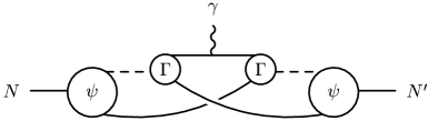
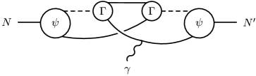
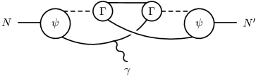
Fig. 2.6: Using the product Ansatz of Eq. (2.3.48), the impulse approximation to the electromagnetic current, Eq. (2.3.46), requires the calculation of these five contributions. $\psi$: $\psi(\ell_{1},\ell_{2})$ in (2.3.48); $\Gamma$: Bethe-Salpeter-like diquark amplitude in (2.3.49); dotted line: $\Delta(K)$, diquark propagator in (2.3.52); solid line: $S(q)$, quark propagator in (2.3.55). The lowest three diagrams, which describe the interchange between the dormant quark and the diquark participants, effect the antisymmetrisation of the nucleon’s Fadde^′ev amplitude. Current conservation follows because the photon-quark vertex is dressed, given in (2.3.31).

The impulse approximation to the electromagnetic current in this model can now be obtained directly from Eq. (2.3.46). This $8$-point Schwinger function expresses a product of eight Grassmann variables and, via an analogue of Wick’s theorem, that can be reduced to a sum of products of four $2$-point dressed-quark Schwinger functions and the dressed-quark-photon vertex, with momenta and indices correlated via Eq. (2.3.48). Using the $1\leftrightarrow 2$ particle exchange symmetry exhibited explicitly by Eq. (2.3.48) one arrives at the result depicted in Fig. 2.6.

The product Ansatz is completely specified once explicit forms for the functions are given and Ref. [162] employs

$$\psi(\ell_{1},\ell_{2}) = \frac{1}{{\cal N}_{\Psi}}\,{\cal F}(\ell^{2}/\omega_{\psi}^{2})\,,\;\ell:=\mbox{\footnotesize$\frac{1}{3}$}\,\ell_{1}-\mbox{\footnotesize$\frac{2}{3}$}\,\ell_{2}\,,$$ (2.3.50)

$$\Gamma(q_{1},q_{2}) = \frac{1}{{\cal N}_{\Gamma}}\,{\cal F}(q^{2}/\omega_{\Gamma}^{2})\,,\;q:=\mbox{\footnotesize$\frac{1}{2}$}\,q_{1}-\mbox{\footnotesize$\frac{1}{2}$}\,q_{2}\,,$$ (2.3.51)

$$\Delta(K) = \frac{1}{m_{\Delta}^{2}}\,{\cal F}(K^{2}/\omega_{\Gamma}^{2})\,,$$ (2.3.52)

$${\cal F}(y) = \frac{1-{\rm e}^{-y}}{y}\,,$$ (2.3.53)

whose parameters were fixed by fitting the proton’s charge form factor on $Q^{2}\in[0,3]\,$GeV² [160]:

$$\begin{array}[]{l|ccc}&\;\omega_{\psi}&\omega_{\Gamma}&m_{\Delta}\\ \hline\cr\mbox{in GeV}&\;0.20&1.4&0.63\end{array}\,,\;\;\;\;\begin{array}[]{l|ccc}&\;1/\omega_{\psi}&1/\omega_{\Gamma}&1/m_{\Delta}\\ \hline\cr\mbox{in fm}&0.99&0.14&0.31\end{array}\,.$$ (2.3.54)

The two tables demonstrate the internal consistency of the model. $d_{\Gamma}:=1/\omega_{\Gamma}$ is a measure of the mean separation between the quarks constituting the scalar diquark and $d_{\psi}:=1/\omega_{\psi}$ is the analogue for the quark-diquark separation. $d_{\Gamma}<d_{\psi}$ is necessary if the quark-quark clustering interpretation is to be valid. $\ell_{(ud)_{0^{+}}}=1/m_{\Delta}$ is a measure of the range over which the diquark persists and that must be significantly less than the nucleon’s diameter. [${\cal N}_{\Psi}$ and ${\cal N}_{\Gamma}$ are the nucleon and $(ud)$ diquark normalisation constants, which are defined and calculated analogously to Eq. (2.3.6), and ensure composite electric charges of $1$ for the proton and $1/3$ for the diquark.]

As is plain in Fig. 2.6, the calculation also involves the dressed-quark propagator and, based on the success of applications such as Refs. [38, 84, 105, 106, 111, 140, 141], the following algebraic parametrisation is employed in Refs. [160, 162]:

$$S(p) = -i\gamma\cdot p\,\sigma_{V}(p^{2})+\sigma_{S}(p^{2})\,,$$ (2.3.55)

$$\bar{\sigma}_{S}(x) = 2\,\bar{m}\,{\cal F}(2(x+\bar{m}^{2}))+{\cal F}(b_{1}x)\,{\cal F}(b_{3}x)\,\left[b_{0}+b_{2}{\cal F}(\epsilon x)\right]\,,$$ (2.3.56)

$$\bar{\sigma}_{V}(x) = \frac{1}{x+\bar{m}^{2}}\,\left[1-{\cal F}(2(x+\bar{m}^{2}))\right]\,,$$ (2.3.57)

$x=p^{2}/\lambda^{2}$, $\bar{m}$ = $m/\lambda$, $\bar{\sigma}_{S}(x)=\lambda\,\sigma_{S}(p^{2})$ and $\bar{\sigma}_{V}(x)=\lambda^{2}\,\sigma_{V}(p^{2})$. The mass-scale, $\lambda=0.566\,$GeV, and parameter values

$$\begin{array}[]{ccccc}\bar{m}&b_{0}&b_{1}&b_{2}&b_{3}\\ \hline\cr 0.00897&0.131&2.90&0.603&0.185\end{array}\;,$$ (2.3.58)

were fixed in a least-squares fit to light-meson observables[137]. [$\epsilon=10^{-4}$ in (2.3.56) acts only to decouple the large- and intermediate-$p^{2}$ domains.] This simple form captures the essential features of direct solutions of Eq. (2.2.1). It represents the dressed-quark propagator as an entire function, which is inspired by the algebraic solutions in Refs. [163, 164] and ensures confinement via the means described in Sec. 2.2; and exhibits DCSB with

$$-\langle\bar{q}q\rangle_{1\,{\rm GeV}^{2}}=\lambda^{3}\,\frac{3}{4\pi^{2}}\,\frac{b_{0}}{b_{1}\,b_{3}}\,\ln\frac{1}{\Lambda_{\rm QCD}^{2}}=(0.221\,{\rm GeV})^{3}\,,$$ (2.3.59)

which is calculated directly from Eqs. (2.2.12), (2.2.48) after noting that Eqs. (2.3.56), (2.3.57) yield the chiral limit quark mass function of Eq. (2.2.47) with $\gamma_{m}=1$. This is a general feature; i.e., the parametrisation exhibits asymptotic freedom at large-$p^{2}$ omitting only the additional $\ln(p^{2}/\Lambda_{\rm QCD}^{2})$-suppression, which is a useful but not necessary simplification. As we see here, this omission introduces model artefacts that are easily identified and accounted for.

Reference [160] obtains a good description of the proton’s charge and magnetic form factors, and also the neutron’s magnetic form factor. The nonpointlike nature of the scalar diquark correlation makes possible a magnetic moment ratio of $|\mu_{n}/\mu_{p}|=0.55$, cf. $0.68$ experimentally. This ratio is always less-than $0.5$ when the correlation is pointlike. The neutron’s charge form factor is poorly described. The charge-radius-squared is negative, consistent with the data, but is $60$% too large. That defect results primarily from neglecting the contribution of the axial-vector diquark.

The nucleon’s scalar form factor is

$$\sigma(q^{2})\,\bar{u}(P^{\prime})u(P):=\langle P^{\prime}|\,m(\bar{u}u+\bar{d}d)\,|P\rangle\,,$$ (2.3.60)

where the nucleon spinors satisfy:

$$\gamma\cdot P\,u(P)=iMu(P)\,,\;\bar{u}(P)\,\gamma\cdot P=iM\bar{u}(P)\,,$$ (2.3.61)

with the nucleon mass $M=0.94\,$GeV, $q=(P^{\prime}-P)$ and $R=(P^{\prime}+P)$. The $\pi N$ $\sigma$-term is just $\sigma(q^{2}=0)$, which is the in-nucleon expectation value of the explicit chiral symmetry breaking term in the QCD Lagrangian. The general form of a fermion-scalar vertex is

$$\Lambda\!\!\!_{\mbox{\large\boldmath$1$}}(q,P)=f_{1}+i\gamma\cdot q\,f_{2}+i\gamma\cdot R\,f_{3}+i\sigma_{\mu\nu}R_{\mu}q_{\nu}\,f_{4}\,,\;f_{i}=f_{i}(q^{2},R^{2})$$ (2.3.62)

since $q\cdot R=0$ for elastic processes. However, using Eqs. (2.3.61) the scalar current simplifies:

$$J_{\mbox{\large\boldmath$1$}}(P^{\prime},P) := \bar{u}(P^{\prime})\Lambda_{\mbox{\large\boldmath$1$}}(q,P)u(P)=s(q^{2})\,\bar{u}(P^{\prime})\,u(P)\,,$$ (2.3.63)

$$s(q^{2}) = f_{1}-2Mf_{3}+q^{2}f_{4}\,.$$ (2.3.64)

The impulse approximation to $J_{\mbox{\large\boldmath$1$}}(P^{\prime},P)$ is also given by the five diagrams in Fig. 2.6 but with the dressed-quark-photon vertex replaced by the dressed-quark-scalar vertex, which is the solution of an inhomogeneous BSE analogous to Eq. (2.3.29). In Ref. [162], to hasten an exemplifying result, the scalar vertex equation was solved using the Goldstone-theorem-preserving separable model of Ref. [114]. In that model the BSE assumes the form

$$\Gamma_{\mbox{\large\boldmath$1$}}(k;Q)=\mbox{\large\boldmath$1$}-\mbox{\footnotesize$\frac{4}{3}$}\int\frac{d^{4}q}{(2\pi)^{4}}\Delta(k-q)\gamma_{\mu}S(q_{+})\Gamma_{\mbox{\large\boldmath$1$}}(q;Q)S(q_{-})\gamma_{\mu}\,,$$ (2.3.65)

with the interaction

$$\Delta(k-q)=G(k^{2})G(q^{2})+k\cdot q\,F(k^{2})F(q^{2})\,,$$ (2.3.66)

where $F(k^{2})$, $G(k^{2})$ are regularised forms of the $A$, $B$ obtained from Eqs. (2.3.56), (2.3.57). [NB. The regularisation ensures convergence of necessary integrals in the separable model.] The solution of Eq. (2.3.65) is

$$\Gamma_{\mbox{\large\boldmath$1$}}(k;Q)=\mbox{\large\boldmath$1$}+t_{1}(Q^{2})\,G(k^{2})+\,i\,t_{2}(Q^{2})\,F(k^{2})\,\frac{k\cdot Q\,\gamma\cdot Q}{Q^{2}}+\,i\,t_{3}(Q^{2})F(k^{2})\,\gamma\cdot k\,.$$ (2.3.67)

The $\sigma$-term is only sensitive to the vertex at $Q^{2}=0$, where the solution reduces to

$$\Gamma_{\mbox{\large\boldmath$1$}}(k;Q)|_{Q^{2}=0}=\mbox{\large\boldmath$1$}+t_{1}(0)\,G(k^{2})+t_{3}(0)\,F(k^{2})\,i\gamma\cdot k\,,$$ (2.3.68)

with $t_{1}(0)=0.242\,$GeV, $t_{3}(0)=-0.0140\,$GeV. Calculation shows that at $k^{2}=0$ the $t_{1}$-term is 6-times larger than the bare term; i.e., it is dominant in the infrared. That is to be expected because it represents the effect of the nonperturbative DCSB mechanism in the solution. This and the other $t_{i}$-terms vanish as $k^{2}\to\infty$, which is just a manifestation of asymptotic freedom.

What makes the inhomogeneous scalar BSE important here is that it has a solution for all $Q^{2}$ and that solution exhibits a pole at the $\sigma$-meson mass; i.e., in the neighbourhood of $(-Q^{2})=m_{\sigma}^{2}=(0.715\,{\rm GeV})^{2}$

$$\Gamma_{\mbox{\large\boldmath$1$}}(k;Q)={\it regular}\;+\frac{n_{\sigma}m_{\sigma}^{2}}{Q^{2}+m_{\sigma}^{2}}\,\Gamma_{\sigma}(k;Q)\,,$$ (2.3.69)

where regular indicates terms that are regular in this neighbourhood and $\Gamma_{\sigma}(k;Q)$ is the canonically normalised $\sigma$-meson Bethe-Salpeter amplitude, whose form is exactly that of $(\Gamma_{\mbox{\large\boldmath$1$}}(k;Q)-\mbox{\large\boldmath$1$})$ in Eq. (2.3.67). This is qualitatively identical to the behaviour of the solution of Eq. (2.3.29) discussed above in connection with $F_{\pi}(Q^{2})$ and elucidated in Refs. [107, 131]. The simple pole appears in each of the functions $t_{i}(Q^{2})$ and a pole fit yields, with $m$ the current-quark mass,

$$m\,n_{\sigma}=3.3\,{\rm MeV}\,.$$ (2.3.70)

$n_{\sigma}m_{\sigma}^{2}$ is the analogue of the residue of the $\pi$-pole in the pseudoscalar vertex, Eq. (2.3.22): $-\sqrt{2}\,\langle\bar{q}q\rangle_{\pi}/f_{\pi}$, and its flow under the renormalisation group is identical. $m\,n_{\sigma}$ is renormalisation point independent and its value can be compared with

$$\frac{-m\langle\bar{q}q\rangle_{\pi}}{\mbox{\footnotesize$\frac{1}{\sqrt{2}}$}f_{\pi}}\,\frac{1}{m_{\sigma}^{2}}=3.6\,{\rm MeV};$$ (2.3.71)

i.e., the magnitude of $n_{\sigma}$ is typical of effects driven by dynamical chiral symmetry breaking. The $\sigma$-meson-$\bar{q}q$ coupling is defined on-shell

$$g_{\sigma\bar{q}q}:=\left.\Gamma_{\sigma}(0;Q)\right|_{Q^{2}=-m_{\sigma}^{2}}=12.6\,,$$ (2.3.72)

and its magnitude can be placed in context via a comparison with $g_{\pi\bar{q}q}=11.8$, which is defined analogously.

The expectation value in Eq. (2.3.60) is obtained with

$$\Gamma_{m}(k;Q)=m\,\Gamma_{\mbox{\large\boldmath$1$}}(k;Q)$$ (2.3.73)

as the probe vertex in Fig. 2.6, and using the solution for $\Gamma_{\mbox{\large\boldmath$1$}}$ described here the calculated $\sigma$-term is [162]

$$\sigma/M_{N}=0.015\,.$$ (2.3.74)

No parameters were varied to obtain this result, which may be compared with a recent lattice computation [165]: $\sigma/M_{N}=0.019\pm 0.05$, calculated using an extrapolation in the current-quark mass. Alternative extrapolation methods can lead to larger values; e.g., $\sigma/M_{N}=0.047$–$0.059$ [166], which are also suggested by some phenomenological analyses [12, 167]. [The $\sigma$-term is not directly accessible via experiment but a value is theoretically inferred by extrapolating $\pi N$ scattering data using dispersion relations [168]: $\sigma/M_{N}=0.047$–$0.076$.] Simple estimates indicate that the result in Eq. (2.3.74) increases with decreasing $m_{\sigma}$, and a reduction in $m_{\sigma}$ is a likely consequence of using an improved kernel in the inhomogeneous scalar BSE. Thus Eq. (2.3.74) is an excellent first estimate.

Fig. 2.7: $\sigma(q^{2})$ as calculated in Ref. [162] using the solution of the inhomogeneous scalar BSE, Eq. (2.3.65). The rapid increase with decreasing $q^{2}$ is associated with the evolution to the $\sigma$-meson pole. A similar feature was also encountered in the calculation of the pion’s electromagnetic form factor, see Fig. 2.4 on page 2.4 and the associated discussion. On this scale, $\sigma(q^{2})$ calculated without the $t_{2,3}(Q^{2})$ contributions is indistinguishable from the full calculation. (Adapted from Ref. [162].)

The nucleon’s scalar form factor is depicted in Fig. 2.7, where the evolution to the $\sigma$-meson pole is evident. Fitting ($t=-q^{2}$)

$$\sigma(t)=g_{\sigma NN}\,\frac{m\,n_{\sigma}}{1-t/m_{\sigma}^{2}}\,,\;t\in[0.1,0.5]\,{\rm GeV}^{2}\,,$$ (2.3.75)

which isolates the residue associated with $\Gamma_{m}(k;Q)$, one obtains the on-shell coupling: $g_{\sigma NN}=27.3$. A direct calculation using the solution of the homogeneous Bethe-Salpeter equation yields $g_{\sigma NN}=27.7$, in agreement within Monte-Carlo errors. Equation (2.3.75) alone overestimates the magnitude of the calculated $\sigma(t)$ everywhere except in the neighbourhood of the pole.

As the lowest-mass pole-solution of a rainbow-ladder BSE, Eq. (2.3.65), the $\sigma$-meson described here is not obviously related to the scalar meson introduced in phenomenological nucleon-nucleon potentials [169, 170] and meson exchange models [171] to mock-up two-pion exchange. However, a coupling relevant to such models can be estimated by introducing $g_{\sigma}(t)$:

$$\sigma(t)=:g_{\sigma}(t)\,\frac{m\,n_{\sigma}}{1-t/m_{\sigma}^{2}}\,,$$ (2.3.76)

where a fit to the calculated $\sigma(t)$ in Fig. 2.7 yields

$$g_{\sigma}(t)=1.61+2.61\,\frac{1}{(1-t/\Lambda_{\sigma}^{2})^{10}}\,,\;\;\Lambda_{\sigma}=1.56\,{\rm GeV}\,,$$ (2.3.77)

with the large exponent merely reflecting the rapid evolution from bound state to continuum dominance of the vertex in the spacelike region. $g_{\sigma}(t)$ describes the $t$-dependent nucleon to scalar-quark-antiquark-correlation coupling strength and at the mock-$\sigma$-mass: $m_{\sigma}^{2\pi}=0.5\,$GeV,

$$g_{\sigma}:=g_{\sigma}((m_{\sigma}^{2\pi})^{2})=9.3\,,$$ (2.3.78)

which may be compared with a phenomenologically inferred value: $g_{\sigma}=10$ [172]. This gives a microscopic interpretation of the mock-$\sigma$. [It is important to note that $g_{\sigma}(4\,m_{\pi}^{2})=5.2$ and hence this comparison is meaningful on a relevant phenomenological domain.] Further, $g_{\sigma}(q^{2}\to\infty)=1.61$ so that $\sigma(q^{2})$ is well approximated by a single monopole for $q^{2}>1\,$GeV². However, the residue is very different from the on-shell value. The scalar radius of the nucleon is obtained from

$$\langle r_{\sigma NN}^{2}\rangle:=-\frac{6}{\sigma}\,\left.\frac{d\sigma(q^{2})}{dq^{2}}\right|_{q^{2}=0}=(0.89\,\mbox{fm})^{2}\,,$$ (2.3.79)

which may be compared with an inferred value [172]: $(1.2\,{\rm fm})^{2}$.

Reference [162] calculates a range of non-electromagnetic nucleon form factors and provides a uniformly good description, yielding meson-nucleon form factors that are “soft” and couplings that generally agree well with those employed in meson-exchange models. Where there are discrepancies with these models or with experiment, a plausible cause and means for its amelioration was readily identified. The study demonstrates that it is realistic to hope for useful constraints on meson-exchange models from well-moulded models of hadron structure. The analysis of the nucleon $\sigma$-term is particularly important because it illustrates the only method that allows an unambiguous off-shell extrapolation in the estimation of meson-nucleon form factors: one must employ solutions of the inhomogeneous BSEs to describe correlations in a channel when the total momentum is not in the neighbourhood of a bound state pole. Improvements to the simple quark$+$scalar-diquark nucleon model are being developed and their application to a wide range of hadronic phenomena is being explored. These studies hold the promise of providing a much-needed standard model of the nucleon.

3 Nonzero Density and Temperature

Identifying the onset and properties of a quark gluon plasma [QGP] is the primary objective of studies at nonzero temperature and density. Such a plasma is expected to be characterised by light quarks and gluons propagating freely over distances $\sim 10$-times larger than the proton. The exploration of QCD in this domain requires a knowledge of equilibrium statistical field theory, for which Sec. 6 of Ref. [105] is a primer and Refs. [173] provide a graduate-level introduction. Here the application of DSEs provides our primary medium and we will describe the necessary and related concepts.

Section 2 reviews the application of DSEs at zero density and temperature. It shows that the framework is efficacious on this domain and well constrained. Both are important because little is known about the domain of high density and/or temperature, and much of what we do know comes from the extrapolation of models. Since the DSEs provide a nonperturbative framework that admits the simultaneous study of DCSB and confinement they are well suited to explore the phase transition that yields the QGP. Furthermore, as they also accurately describe bound states, they can be used to explore the response of hadron properties to extremes of density and temperature; i.e., to elucidate signals of QGP formation. These features also mean that the DSEs can address all the phenomena accessible in lattice-QCD simulations and therefore they can be used to confirm the results of such studies. Importantly too the lattice simulations can be used to constrain the model-dependent elements of DSE studies, making possible a reliable DSE extrapolation into the domain of nonzero chemical potential QCD, for example, which is inaccessible in contemporary lattice-QCD.

3.1 In-medium Essentials

Equation of State       The $T\neq 0$ analogue of the partition function in Eq. (2.1.9) is

$${\cal Z}_{(\mu,T)}[\bar{\eta},\eta,J]=\int d\mu_{\beta}(\bar{q},q,A,\bar{\omega},\omega)\,\exp\int_{0}^{\beta}\!d\tau\int\!d^{3}x\left[\bar{q}\,\eta+\bar{\eta}\,q+J_{\mu}^{a}\,A_{\mu}^{a}\right],$$ (3.1.1)

with $x_{4}\to\tau$, $\beta:=1/T$ and the measure

$$d\mu_{\beta}(\bar{q},q,A,\bar{\omega},\omega):=$$

$$\prod_{\vec{x}\tau\in[0,\beta]}\prod_{\phi}{\cal D}\bar{q}_{\phi}(\vec{x},\tau){\cal D}q_{\phi}(\vec{x},\tau)\prod_{a}{\cal D}\bar{\omega}^{a}(\vec{x},\tau){\cal D}\omega^{a}(\vec{x},\tau)\prod_{\mu}{\cal D}A_{\mu}^{a}(\vec{x},\tau)\exp(-S_{\beta}[\bar{q},q,A]-S_{\beta}^{g}[\bar{\omega},\omega,A])\,,$$

where $S_{\beta}[\bar{q},q,A]$, $S_{\beta}^{g}[\bar{\omega},\omega,A]$ are the actions of Eqs. (2.1.8), (2.1.12) but for the obvious bounding of the $\tau$-integral. The frame specified by separating the spacetime integral into a product of a compact integral over Euclidean time and the volume integral is not prescribed by the theory. This separation breaks the theory’s original $O(4)$ symmetry to $O(3)$ and is effected by introducing an arbitrary, normalised, spacelike vector, $u_{\mu}$, with $u\cdot p=0$ defining the $T=0$-hyperplane. Here we have employed a conventional choice for the heat bath vector: $u=(\vec{0},1)$. [NB. The zero temperature theory is recovered by taking the limit $T\to 0$; i.e., $\beta\to\infty$, in Eqs. (3.1.1), (3.1).] The chemical potential is introduced as a Lagrange multiplier

$$S_{\beta}[\bar{q},q,A]\to S_{\mu,\beta}[\bar{q},q,A]:=S_{\beta}[\bar{q},q,A]-\int_{0}^{\beta}\!d\tau\int\!d^{3}x\,\mu\,\bar{q}\gamma_{4}q\,.$$ (3.1.3)

With $\mu\neq 0$, $S_{\mu,\beta}[\bar{q},q,A]$ is not Hermitian and hence $d\mu_{\mu,\beta}$ is not a probability measure. That makes numerical simulations of lattice-regularised $\mu\neq 0$ QCD very difficult; in fact, there is currently no satisfactory algorithm [174]. The functional integral in Eq. (3.1.1) is evaluated on the space of Grassmann fields for which $q(\vec{x},0)=-q(\vec{x},\beta)$; i.e., over fields satisfying antiperiodic boundary conditions, and over gauge fields satisfying periodic boundary conditions. These boundary conditions are an essential aspect of the difference between fermion and boson statistics.

The partition function is particularly important in equilibrium statistical field theory. As usual, it yields the DSEs in a straightforward manner, however, more than that, all the thermodynamic functions are obtained from the partition function. The thermodynamic potential and pressure densities are

$$-\omega(\mu,T)=p(\mu,T)=\frac{1}{\beta V}\ln{\cal Z}_{(\mu,T)}\,,$$ (3.1.4)

where $\beta V$ is the four-volume normalising factor. The stable phase of the system is that in which the pressure is maximal or equivalently the thermodynamic potential energy is minimised. The expression for the pressure is the Equation of State [EOS] and from that one immediately obtains the baryon number and entropy densities:

$$\rho(\mu,T)=\left.\frac{\partial}{\partial\mu}\,p(\mu,T)\right|_{T\,{\rm fixed}}\!,\;\;\;s(\mu,T)=\left.\frac{\partial}{\partial T}\,p(\mu,T)\right|_{\mu\,{\rm fixed}}$$ (3.1.5)

and also the energy density:

$$\epsilon(\mu,T)=-p(\mu,T)+\mu\,\rho(\mu,T)+T\,s(\mu,T)\,.$$ (3.1.6)

The calculation of these quantities in QCD is a contemporary focus; e.g., Refs. [175, 176, 177].

A simple estimate of the pressure due to dressed-quarks is obtained via the “steepest descent” approximation, which yields

$$p_{\Sigma}(\mu,T)=\frac{1}{\beta V}\left\{{\rm TrLn}\left[\beta S^{-1}\right]-\mbox{\footnotesize$\frac{1}{2}$}{\rm Tr}\left[\Sigma\,S\right]\right\},$$ (3.1.7)

where $S$ is the solution of the gap equation with $\Sigma$ the associated self energy, and “Tr” and “Ln” are extensions of “tr” and “$\ln$” to matrix-valued functions. Equation (3.1.7) is just the auxiliary field effective action [178], which yields the free fermion pressure in the absence of interactions; i.e., when $\Sigma\equiv 0$. At this level of truncation the total pressure receives an additive contribution from dressed-gluons:

$$p_{\Delta}(\mu,T)=-\frac{1}{\beta V}\,\mbox{\footnotesize$\frac{1}{2}$}{\rm TrLn}\left[\beta^{2}D_{\mu\nu}^{-1}\right]\,,$$ (3.1.8)

where $D_{\mu\nu}$ is the $T\neq 0$ dressed-gluon $2$-point function, and this yields the free-gluon pressure in the absence of interactions.

Propagators       As just described, the introduction of temperature to Euclidean QCD breaks the original $O(4)$ symmetry to $O(3)$. In this case the most general form of the dressed-quark propagator is [179]

$$S(p,u)^{-1}=i\gamma\cdot p\,a(p^{2},[u\cdot p]^{2})+b(p^{2},[u\cdot p]^{2})+i\gamma\cdot u\,u\cdot p\,c(p^{2},[u\cdot p]^{2})+i\sigma_{\mu\nu}p_{\mu}u_{\nu}\,d(p^{2},[u\cdot p]^{2})\,,$$ (3.1.9)

where $u_{\mu}=(\vec{0},1)$, and the surviving $O(3)$ invariance of Eq. (3.1.9) is apparent upon inspection. Even at $T\neq 0$, the chiral-limit dressed-quark propagator should satisfy

$$V(\alpha)\,S(p,u)^{-1}\,V(\alpha)=S(p,u)^{-1}\,,\;\;V(\alpha)=\exp\left(i\gamma_{5}\,\mbox{\footnotesize$\frac{1}{2}$}\lambda_{F}^{l}\alpha^{l}\right)\,,$$ (3.1.10)

if chiral symmetry is realised in the Wigner-Weyl mode. Hence $b\equiv 0\equiv d$ in this case. Furthermore, since the term involving $d$ does not appear in the free fermion action of thermal field theory, there are no perturbative divergences in this function’s evaluation and $d$ is therefore power-law suppressed in the ultraviolet. [cf. The discussion of the chiral limit fermion mass function on page 2.2.13.] These features, along with the vector exchange nature of the interaction, underly the fact that $d(p^{2},u\cdot p^{2})$ only plays a minor role in the solution of the QCD gap equation. Hereafter we neglect it and assume the following as the most general form of the dressed-quark $2$-point function:

$$S(\vec{p},\tilde{\omega}_{k}) = \frac{1}{i\vec{\gamma}\cdot\vec{p}\,A(\vec{p}\,^{2},\tilde{\omega}_{k}^{2})+B(\vec{p}\,^{2},\tilde{\omega}_{k}^{2})+i\gamma_{4}\,\tilde{\omega}_{k}C(\vec{p}\,^{2},\tilde{\omega}_{k}^{2})}\,,$$ (3.1.11)

$$= -i\vec{\gamma}\cdot\vec{p}\,\sigma_{A}(\vec{p}\,^{2},\tilde{\omega}_{k}^{2})+\sigma_{B}(\vec{p}\,^{2},\tilde{\omega}_{k}^{2})-i\gamma_{4}\,\tilde{\omega}_{k}\sigma_{C}(\vec{p}\,^{2},\tilde{\omega}_{k}^{2})\,,$$ (3.1.12)

where $\tilde{\omega}_{k}=\omega_{k}+i\mu$, with $\mu$ the chemical potential, and $\omega_{k}=(2k+1)\,\pi T$, $k\in Z\!\!\!\!Z$, are the fermion Matsubara frequencies, which ensure $q(\vec{x},0)=-q(\vec{x},\beta)$. The scalar functions: ${\cal F}=A$, $B$, $C$, are complex and satisfy

$${\cal F}(\vec{p}\,^{2},\tilde{\omega}_{k}^{2})^{\ast}={\cal F}(\vec{p}\,^{2},\tilde{\omega}_{-k-1}^{2})\,.$$ (3.1.13)

[NB. The functions $A$, $C$ cannot be neglected. For $T=0$, $A=C$ and $A-1\not\equiv 0$; e.g., Refs. [20, 45], and the momentum dependence of $A$ can conspire with that of $B$ to ensure confinement of dressed-quarks [164]. Furthermore, as will become clear, the $(\vec{p}\,^{2},\tilde{\omega}_{k}^{2})$-dependence of $A$, $C$ has a marked effect on the behaviour of bulk thermodynamic quantities.]

The dressed-quark $2$-point function satisfies a gap equation

$$S(p_{\omega_{k}})^{-1}=Z_{2}^{A}\,i\vec{\gamma}\cdot\vec{p}+Z_{2}\,(i\gamma_{4}\,\tilde{\omega}_{k}+m_{\rm bare})\,+\Sigma^{\prime}(p_{\omega_{k}})\,,$$ (3.1.14)

which can be derived in the usual way from the partition function, Eq. (3.1.1). Here we have introduced a shorthand notation: $p_{\omega_{k}}=(\vec{p},\tilde{\omega}_{k})$, and the regularised self energy is

$$\Sigma^{\prime}(p_{\omega_{k}}) = i\vec{\gamma}\cdot\vec{p}\,\Sigma_{A}^{\prime}(p_{\omega_{k}})+i\gamma_{4}\,\omega_{k}\,\Sigma_{C}^{\prime}(p_{\omega_{k}})+\Sigma_{B}^{\prime}(p_{\omega_{k}})\,,$$ (3.1.15)

$$\Sigma_{\cal F}^{\prime}(p_{\omega_{k}}) = \mbox{\footnotesize$\frac{1}{4}$}{\rm tr}\,{\cal P}_{\cal F}\int_{l,q}^{\bar{\Lambda}}\,\mbox{\footnotesize$\frac{4}{3}$}\,g^{2}\,D_{\mu\nu}(\vec{p}-\vec{q},\omega_{k}-\omega_{l})\,\gamma_{\mu}S(q_{\omega_{l}})\Gamma_{\nu}(q_{\omega_{l}};p_{\omega_{k}})\,,$$ (3.1.16)

where the renormalisation factors are ${\cal P}_{A}:=-(Z_{1}^{A}/|\vec{p}|^{2})i\vec{\gamma}\cdot\vec{p}$, ${\cal P}_{B}:=Z_{1}$, ${\cal P}_{C}:=-(Z_{1}/\omega_{k})i\gamma_{4}$, and $\int_{l,q}^{\bar{\Lambda}}:=\,T\,\sum_{l=-\infty}^{\infty}\,\int^{\bar{\Lambda}}d^{3}q/(2\pi)^{3}$, with $\int^{\bar{\Lambda}}$ representing a translationally invariant regularisation of the three-dimensional integral and $\bar{\Lambda}$ is the regularisation mass-scale. Since introducing $\mu$, $T$ does not generate qualitatively new divergences, the regularisation and renormalisation proceeds just as in the absence of the medium so that the renormalised self energies are

$$\begin{array}[]{rcl}{\cal F}(p_{\omega_{k}};\zeta)&=&\xi_{\cal F}+\Sigma_{\cal F}^{\prime}(p_{\omega_{k}};{\bar{\Lambda}})-\Sigma_{\cal F}^{\prime}(\zeta^{-}_{\omega_{0}};{\bar{\Lambda}})\,,\end{array}$$ (3.1.17)

with $\zeta$ the renormalisation point, $(\zeta^{-}_{\omega_{0}})^{2}:=\zeta^{2}-\omega_{0}^{2}$, $\xi_{A}=1=\xi_{C}$, and $\xi_{B}=m_{R}(\zeta)$. [cf. Eqs. (2.2.39-2.2.43).]

The regularised self energy is expressed in terms of the renormalised dressed-gluon $2$-point function and dressed-quark-gluon $3$-point function. At $T\neq 0$ in Landau gauge the complete expression of the former requires two $O(3)$-scalar functions [cf. Eq. (2.2.15)]

$$g^{2}D_{\mu\nu}(p_{\Omega_{k}})=P_{\mu\nu}^{L}(p_{\Omega_{k}})\Delta_{F}(p_{\Omega_{k}})+P_{\mu\nu}^{T}(p_{\Omega_{k}})\Delta_{G}(p_{\Omega_{k}})\,,$$ (3.1.18)

where $p_{\Omega_{k}}:=(\vec{p},\Omega_{k})$, $\Omega_{k}=2k\pi T$ is the Matsubara frequency for bosons, and

$$P_{\mu\nu}^{T}(p_{\Omega_{k}}) := \left\{\begin{array}[]{ll}0,&\mu\;{\rm and/or}\;\nu=4,\\ \displaystyle\delta_{ij}-\frac{p_{i}p_{j}}{p^{2}},&\mu,\nu=i,j\,=1,2,3\;,\end{array}\right.$$ (3.1.21)

$$P_{\mu\nu}^{L}(p_{\Omega_{k}}) = \delta_{\mu\nu}-\frac{p_{\mu}p_{\nu}}{p^{2}}-P_{\mu\nu}^{T}(p_{\Omega_{k}})\,.$$ (3.1.22)

In the absence of interactions: $\Delta_{F}(p_{\Omega_{k}}^{2})=\Delta_{G}(p_{\Omega_{k}})=1/p_{\Omega_{k}}^{2}$. The QCD analogue of a Debye [or electric screening] mass appears as a $T$-dependent contribution to $\Delta_{F}$, the gluon’s longitudinal polarisation function. The complete expression of the renormalised dressed-quark-gluon $3$-point function requires at least fifty-four scalar functions [cf. twelve for $T=0$] but, since the theory is renormalisable, ultraviolet divergences are only encountered in evaluating two of them. It follows from this that sensible, character-preserving truncations are possible.

Order Parameters       In order to demarcate the QGP phase it is necessary to identify order parameters; i.e., find operators $X_{i}$ whose expectation values are nonzero in the normal phase: $\langle X_{i}\rangle\neq 0$, but vanish in the QGP: $\langle X_{i}\rangle\equiv 0$. This is often a difficult task. Having identified such operators then, if $\langle X_{i}\rangle$ is discontinuous at the transition point we will describe the transition as first order; otherwise we classify it as second order.

In Sec. 2.2 we described the phenomenon of DCSB and its connection with the purely nonperturbative generation of a scalar term in the dressed-quark self energy when the current-quark mass is zero. One characteristic of this effect is the large magnitude, Eq. (2.2.51), of the vacuum quark condensate that appears in Eqs. (2.2.47), (2.2.48), which has many observable consequences; e.g., it is the primary cause of what is naively an unexpectedly large $\pi$-$\rho$ mass splitting. DCSB is a defining feature of the normal phase of QCD. If, with increasing $\mu$ and/or $T$, the condensate vanishes at some particular value of these parameters then a new phase of QCD has been reached. It is a phase in which chiral symmetry is realised explicitly and, as weakly interacting systems cannot support condensate formation, this is plainly a good defining property of a QGP. The discussion of the chiral limit, Eqs. (2.2.45-2.2.52), also makes plain that it is not possible to have a nonzero quark condensate unless the dressed-quark mass function, $M(p_{\omega_{k}})$, is nonzero too. Therefore the magnitude of this function at any single point is also an order parameter appropriate for characterising the chiral symmetry restoring aspect of the QGP transition. In fact, in DSE studies it is by far the most direct, since it appears in all the integrands that describe other quantities.

We also discussed an arguably more significant aspect of cold, sparse QCD, namely confinement. It is easy to build a model that exhibits DCSB without confinement; e.g., Refs. [12, 13, 14, 180]. However, building a covariant model with confinement and an uncomplicated realisation of all aspects of DCSB is a challenging task. As emphasised by the study of QED₃ in Ref. [88], that challenge is met with a modicum of success using the DSE truncation scheme explored in Ref. [108] and the realisation of confinement via a violation of reflection positivity by coloured $n$-point functions. This also exposes a simple deconfinement order parameter appropriate to both light- and heavy-quarks, whose application is illustrated in Fig. 2.3. To make it plain we return to $D(T)$ defined in Eq. (2.2.72). When calculated from a Schwinger function with complex conjugate poles, $D(T)$ has at least one zero. Denote its position by $T_{0}^{z_{1}}$ and define

$$\kappa_{0}:=1/T_{0}^{z_{1}}\,.$$ (3.1.23)

If, with increasing $\mu$ and/or $T$, one observes $\kappa_{0}$ approaching zero then the [first] zero in $D(T)$ is moving to $T=\infty$. This evolution of $\kappa_{0}$ corresponds to the limiting case when there is no zero at all, which is just the free, unconfined particle described by $\sigma_{S}(T)$ in Eqs. (2.2.67). Thus $\kappa_{0}$ is a good order parameter for deconfinement [181]: it is nonzero in the confined phase, and remains nonzero until the Schwinger function evolves into one that respects reflection positivity and corresponds to an asymptotic state. It is clear that deconfinement is also a good defining property of a QGP.

Critical Behaviour       In second order transitions the length scale associated with correlations in the system diverges as the order parameter vanishes and a range of critical exponents can be defined that characterise the behaviour of macroscopic properties at the transition point. In the context of QCD this can be elucidated via the free energy, which here we write as $f(t,h)$, where $t:=T/T_{c}-1$ is the reduced temperature, with $T_{c}$ a putative critical temperature, and $h:=\beta m_{R}$ is the source of explicit chiral symmetry breaking measured in units of the temperature. [We omit the chemical potential for now so that $f=\epsilon=(T^{2}/V)(\partial\ln{\cal Z}_{(T)}/\partial T)$.] $h$ plays a role analogous to that of an external magnetic field applied to a ferromagnet. Since correlation lengths diverge it follows that for $t,h\to 0$ the free energy is a generalised homogeneous function; i.e.,

$$f(t,h)=\frac{1}{b}\,f(t\,b^{y_{t}},h\,b^{y_{h}})\,.$$ (3.1.24)

As a consequence the “magnetisation” behaves as follows:

$$M(t,h):=\left.\frac{\partial\,f(t,h)}{\!\!\!\!\!\!\partial h}\right|_{t\;{\rm fixed}}\!\!,\;\;\;M(t,h)=b^{y_{h}-1}\,M(t\,b^{y_{t}},h\,b^{y_{h}})\,.$$ (3.1.25)

[NB. Using the partition function one finds easily that $M(t,h)$ is just the vacuum quark condensate. In these formulae it can be replaced by any equivalent order parameter.] The scaling parameter: $b$, is arbitrary and along the trajectory $|t|b^{y_{t}}=1$ one has

$$M(t,h)=|t|^{(1-y_{h})/y_{t}}\,M({\rm sgn}(t),h\,|t|^{-y_{h}/y_{t}})\,;\;\;{\rm i.e.,}\;\;M(t,0)\propto|t|^{\beta}\,,\;\beta:=\frac{1-y_{h}}{y_{t}}\,.$$ (3.1.26)

Alternatively, along the trajectory $hb^{y_{h}}=1$

$$M(t,h)=h^{(1-y_{h})/y_{h}}\,M(t\,h^{-y_{t}/y_{h}},1)\,;\;\;{\rm i.e.,}\;\;M(0,h)\propto h^{1/\delta}\,,\;\delta:=\frac{y_{h}}{1-y_{h}}\,.$$ (3.1.27)

Equations (3.1.26), (3.1.27) quantify the behaviour to be expected of an order parameter at a second order transition. They also introduce two critical exponents and, using the renormalisation group, scaling laws can be derived that relate all other such exponents to $\beta$ and $\delta$ [182]. It is widely conjectured that the values of these exponents are fully determined by the dimension of space and the nature of the order parameter. This is the notion of universality ; i.e., that the critical exponents are independent of a theory’s microscopic details and hence all theories can be grouped into a much smaller number of universality classes according to the values of their critical exponents. If this is the case, the behaviour of a complicated theory near criticality is completely determined by the behaviour of a simpler theory in the same universality class. In mean-field theories

$$\beta^{\rm MF}=\mbox{\footnotesize$\frac{1}{2}$}\,,\;\;\delta^{\rm MF}=3.0\,.$$ (3.1.28)

The success of the nonlinear $\sigma$-model in describing long-wavelength pion dynamics underlies a conjecture [183] that chiral symmetry restoration at $T\neq 0$ in 2-flavour QCD is a second order transition with the theory lying in the universality class characterised by the 3-dimensional, $N=4$ Heisenberg magnet [$O(4)$ model] whose critical exponents are [184]:

$$\beta^{H}=0.38\pm 0.01\,,\;\;\delta^{H}=4.82\pm 0.05\,.$$ (3.1.29)

As an alternative to Eqs. (3.1.26), (3.1.27), the critical exponents can be determined by studying the pseudocritical behaviour of the chiral and thermal susceptibilities:

$$\chi_{h}(t,h):=\left.\frac{\partial\,M(t,h)}{\!\!\!\!\!\!\partial h}\right|_{t\;{\rm fixed}}\!,\;\;\;\chi_{t}(t,h):=\left.\frac{\partial\,M(t,h)}{\!\!\!\!\!\!\partial t}\right|_{h\;{\rm fixed}}\!,$$ (3.1.30)

which are smooth functions of $t$ with maxima at the pseudocritical points: $t_{\rm pc}^{h}$ and $t_{\rm pc}^{t}$, where $t_{\rm pc}^{h}\propto\,h^{1/(\beta\delta)}\,\propto\,t_{\rm pc}^{t}$. Since $\beta\delta>0$, the pseudocritical points approach the critical point: $t=0$, as $h\to 0^{+}$ and

$$\chi_{h}^{\rm pc}:=\chi_{h}(t_{\rm pc}^{h},h)\propto h^{-z_{h}}\,,\;z_{h}:=1-\frac{1}{\delta}\,,\;\;\chi_{t}^{\rm pc}:=\chi_{t}(t_{\rm pc}^{t},h)\propto h^{-z_{t}}\,,\;z_{t}:=\frac{1}{\beta\delta}\,(1-\beta)\,.$$ (3.1.31)

[The appendix of Ref. [185] provides a demonstration.] Mean field behaviour corresponds to

$$z_{h}^{\rm MF}=\mbox{\footnotesize$\frac{2}{3}$}\,,\;\;z_{t}^{\rm MF}=\mbox{\footnotesize$\frac{1}{3}$}\,.$$ (3.1.32)

Analysing the susceptibilities can provide more accurate results when numerical noise is anticipated, which is why the method has been used in lattice-QCD analyses [175].

3.2 Quark Gluon Plasma Phase

Temperature       We are now in a position to describe the application of DSEs to demarcating the QGP and exploring its properties. For the moment we persist with $\mu=0$ and explore the temperature induced transition because that is the domain on which the most complete studies exist [in all approaches].

The properties of the class of rainbow-ladder models are elucidated in Ref. [186]. This class is defined by Eq. (2.2.33) with the mutually consistent $T\neq 0$ constraints: $Z_{1}=Z_{2}$, $Z_{1}^{A}=Z_{2}^{A}$. [NB. The rainbow truncation is the leading term in a $1/N_{c}$-expansion of $\Gamma_{\nu}(q_{\omega_{l}};p_{\omega_{k}})$.] The form of $D_{\mu\nu}(p_{\Omega_{k}})$ has no bearing on whether or not a model is in the class. To be concrete, Ref. [186] considered models defined by

$$\Delta_{F}(p_{\Omega_{k}}) = {\cal D}(p_{\Omega_{k}};m_{g})\,,\;\Delta_{G}(p_{\Omega_{k}})={\cal D}(p_{\Omega_{k}};0)\,,$$ (3.2.1)

$${\cal D}(p_{\Omega_{k}};m_{g}) := 2\pi^{2}D\,\mbox{\footnotesize$\frac{2\pi}{T}$}\delta_{0\,k}\,\delta^{3}(\vec{p})+{\cal D}_{\rm M}(p_{\Omega_{k}};m_{g})\,,$$ (3.2.2)

with three choices of ${\cal D}_{\rm M}(p_{\Omega_{k}};m_{g})$. The first term in ${\cal D}(p_{\Omega_{k}};m_{g})$ is a simple $T\neq 0$ generalisation of the distribution in Eq. (2.2.35). It represents the long-range piece of the effective interaction and the ${\cal D}_{\rm M}(p_{\Omega_{k}};m_{g})$ are chosen so as not to pollute that. (NB. $\Delta_{G}$ does not contain a simple $T$-dependent mass. Such “magnetic” screening is more complicated than electric screening because of infrared divergences in QCD [173].) The three choices are:
    A) ${\cal D}_{\rm M:=A}(p_{\Omega_{k}};m_{g})\equiv 0$, with $D:=\eta^{2}/2$ and $\eta=1.06$ fixed [33] by fitting $\pi$- and $\rho$-meson masses at $T=0$. $m=12\,$MeV yields $m_{\pi}=140\,$MeV. ${\cal D}_{\rm A}$ yields an ultraviolet finite model and hence the renormalisation point and cutoff can be removed simultaneously. Nevertheless it exhibits many features in common with more sophisticated Ansätze [176].
    B) The model of Ref. [181], obtained with $D:=(8/9)\,m_{t}^{2}$ and

$${\cal D}_{\rm M:=B}(p_{\Omega_{k}};m_{g})=\mbox{\footnotesize$\frac{16}{9}$}\pi^{2}\,\frac{1-{\rm e}^{-s_{\Omega_{k}}/(4m_{t}^{2})}}{s_{\Omega_{k}}}\,,$$ (3.2.3)

$s_{\Omega_{k}}:=p_{\Omega_{k}}^{2}+m_{g}^{2}$, where, following Ref. [187], $m_{g}^{2}=4\pi^{2}\gamma_{m}(N_{c}/3+N_{f}/6)=(8/3)\,\pi^{2}T^{2}$ [$N_{f}=3$]. The mass-scale $m_{t}=0.69\,{\rm GeV}=1/0.29\,{\rm fm}$ marks the boundary between the perturbative and nonperturbative domains, and was also fixed [48] by fitting $\pi$- and $\rho$-meson properties at $T=0$. At $\zeta=9.5\,$GeV, $m_{R}=1.1\,$MeV yields $m_{\pi}=140\,$MeV. This model adds a Coulomb-like short-range interaction to that of Ref. [176], thereby marginally improving its ultraviolet behaviour.
    C) A minimal $T\neq 0$ extension of the effective interaction in Eq. (2.2.35) with the only modification being $k^{2}\to s_{\Omega_{k}}$, $m_{g}^{2}=(16/5)\,\pi^{2}T^{2}$, in the last two terms. [Recall that this model’s parameters were fitted with $N_{f}=4$]. As described above, ${\cal D}_{\rm C}$ ensures that the model preserves the one-loop renormalisation group behaviour of QCD. To further explore model-dependence, two parameter sets were employed in Ref. [186], which differ only in the value of $\omega$: ${}_{1}\omega=0.6\,m_{t}$, ${}_{2}\omega=1.2\,m_{t}$. They are equivalent, yielding the same values for pion observables: with ${}_{1}\omega$, a renormalisation point invariant current-quark mass of $\hat{m}=6.6\,$MeV yields $m_{\pi}=140\,$MeV; while with ${}_{2}\omega$, $\hat{m}=5.7\,$MeV effects that.

Two chiral order parameters were employed in analysing chiral symmetry restoration

$${\cal X}:=B(\vec{p}=0,\omega_{0}),\;{\cal X}_{C}:=\frac{B(\vec{p}=0,\omega_{0})}{C(\vec{p}=0,\omega_{0})}.$$ (3.2.4)

They should be equivalent and the onset of that equivalence determines the $h$-domain on which Eqs. (3.1.31) are valid. These being bona fide order parameters is useful and particularly important because it means that the lowest Matsubara frequency completely determines the character of the chiral phase transition, as conjectured in Ref. [188]. Furthermore, it was numerically verified in Ref. [186] that in the chiral limit and for $t\sim 0$: $f_{\pi}\propto\langle\bar{q}q\rangle\propto{\cal X}(t,0)$; i.e., these quantities are all bona fide order parameters.

Table 3.1: Critical temperature for chiral symmetry restoration and critical exponents characterising the second-order transition in the four exemplary models. Averaging over the independent models yields $T_{c}=154\pm 24\,$MeV. (Adapted from Ref. [186].)

$$\begin{array}[]{lcccc}{\rm Model}&{\rm A}&{\rm B}&{\rm C}_{{}_{1}\omega}&{\rm C}_{{}_{2}\omega}\\ \hline\cr T_{c}(MeV)&169&174&120&152\\ z_{h}&0.666&0.67\pm 0.01&0.667\pm 0.001&0.669\pm 0.005\\ z_{t}&0.335&0.33\pm 0.02&0.333\pm 0.001&0.33\pm 0.01\\ \hline\cr\end{array}$$

The results for the critical temperature and exponents are presented in Table 3.1, where the quoted critical temperatures are easily determined using either Eqs. (3.1.26), (3.1.27) or $t_{\rm pc}^{h}\propto\,h^{1/(\beta\delta)}\,\propto\,t_{\rm pc}^{t}$. The models are all constrained by observables in two-flavour QCD and the critical temperature agrees with the current estimate from simulations of lattice-QCD with two dynamical light-quark flavours [175]. (Quenched lattice-QCD exhibits a first order [deconfining] transition at a much higher critical temperature: $T_{c}^{\rm quench}=270(5)\,$MeV [175, 189].) Studies using simple versions of the Nambu–Jona-Lasinio model typically yield higher values: $T_{c}\mathrel{\hbox to0.0pt{\lower 4.0pt\hbox{\hskip 0.0pt$\sim$}\hss}\raise 1.0pt\hbox{$>$}}200\,$MeV [14]. However, that is likely a model artefact. Modifications that make possible a relaxation of the overly restrictive connection between the model’s mass-scale and the dressed-quark mass; such as $1/N_{c}$-[or meson-loop-]corrections or replacing the contact interaction by a separable form, can easily effect a reduction of the critical temperature by $\mathrel{\hbox to0.0pt{\lower 4.0pt\hbox{\hskip 0.0pt$\sim$}\hss}\raise 1.0pt\hbox{$<$}}25$%; e.g., Refs. [190, 191, 192, 193]. This sort of reduction brings it in-line with the estimate in Table 3.1.

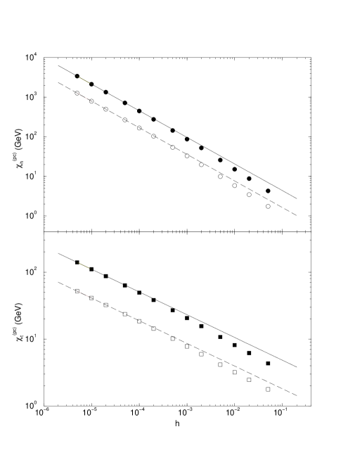
Fig. 3.1: $h$-dependence of the maxima of the chiral (circles) and thermal (squares) susceptibilities calculated with the effective interaction of Eq. (3.2.2) using ${\cal D}_{C}$ with $\omega=1.2\,m_{t}$. The filled symbols are obtained from ${\cal X}$ and the open from ${\cal X}_{C}$, Eq. (3.2.4). The slope of the straight lines is given in Table 3.1 and they are drawn through the two smallest $h$-values, which is explained in the discussion of Eq. (3.2.5). (Adapted from Ref. [186].)

The behaviour of the pseudocritical maxima in the chiral and thermal susceptibilities is illustrated in Fig. 3.1. It is plain that the results exhibit curvature and hence the scaling relations of Eq. (3.1.31) are not satisfied on the entire domain. The domain on which they are valid may be established by defining a “local” critical exponent:

$$z_{i}:=\,-\,\frac{\ln\chi^{\rm pc}_{i}-\ln\chi^{\rm pc}_{i+1}}{\ln h_{i}-\ln h_{i+1}}\,,$$ (3.2.5)

where $(h_{i},\chi^{\rm pc}_{i})$ and $(h_{i+1},\chi^{\rm pc}_{i+1})$ are adjacent data pairs. $h$ lies in the scaling region when $z_{i}$ is independent of the order parameter. Applying this to the ${\cal D}_{\rm B}$ model yields the results in Fig. 3.2, which indicate clearly that the scaling relations are not valid until

$$\log_{10}(h/h_{u})<-7\,,$$ (3.2.6)

where $h_{u}:=m_{R}/T_{c}$ is defined with the current-quark mass that gives $m_{\pi}=140\,$MeV in this model. Applying the same method to the renormalisation-group improved models, ${\cal D}_{\rm C}$, shows that in these cases the scaling relations are only valid for

$${}_{1}\omega\!:\,\log_{10}(h/h_{u})<-5\,, {}_{2}\omega\!:\,\log_{10}(h/h_{u})<-6\,;$$ (3.2.7)

i.e., for current-quark masses six orders of magnitude smaller than those of real $u$,$d$-quarks.

While these are model studies the result is also likely to be true in QCD; i.e., while the critical temperature is relatively easy to determine, very small current-quark masses may be necessary to accurately calculate the critical exponents from the chiral and thermal susceptibilities. If that is the case, the calculation of these exponents via numerical simulations of lattice-QCD will not be feasible. The lattice-to-lattice variation of the critical exponents described in Refs. [175, 189], with even a first order transition being possible, could be a signal of this.

Fig. 3.2: $z_{i}^{h}$ (circles) and $z_{i}^{t}$ (squares) from Eq. (3.2.5) calculated with the effective interaction of Eq. (3.2.2) using ${\cal D}_{B}$ in Eq. (3.2.3): filled symbols - ${\cal X}$, open symbols - ${\cal X}_{C}$. The dashed lines are the mean field values: $z_{h}=2/3$, $z_{t}=1/3$. (Adapted from Ref. [186].)

It is clear from Table 3.1 that each of the models considered in Ref. [186] is mean field in nature. As the long-range part of the effective interaction is identical in each case and the correlation length diverges as $t\to 0$, that may not be surprising. The models are distinguished by the feature that they describe the long-wavelength dynamics of QCD very well, with mesons represented as nonpointlike quark-antiquark composites. Coulomb gauge models [187] also describe mesons as composites and exhibit mean field critical exponents. The long-range part of the interaction there corresponds directly to the regularised Fourier amplitude of a linearly rising potential and therefore it is in no simple way equivalent to the distribution in Eq. (2.2.35). Separable models with [191]: ${\cal D}(p_{\omega_{k}}-q_{\omega_{l}};m_{g})\propto g(|\vec{p}|)\,g(|\vec{q}|)$, where $g(|\vec{p}|)$ is a non-increasing function of its argument, can also provide a good description of long-wavelength pion dynamics. They too describe mesons as composites and exhibit an explicit fermion substructure, and they also have mean field critical exponents, as do models with $g=g(\omega_{k}^{2}+\vec{p}\,^{2})$ [194]. [NB. The Nambu–Jona-Lasinio model can be viewed as a separable model obtained with $g(|\vec{p}|)=\theta(1-|\vec{p}|/_{3}\!\Lambda)$, where ${}_{3}\!\Lambda$ is a cutoff parameter. Also, in the rainbow-truncation DSE model of Ref. [195], which employs an infrared-finite effective interaction, the critical exponent obtained from ${\cal X}$ is $1/2$. However, a different exponent is reported to be obtained from $\langle\bar{q}q\rangle$. We expect that is erroneous, as these must be equivalent order parameters.]

All these examples are members of the class of rainbow truncation models. Therefore the results indicate that chiral symmetry restoration in this class is a mean field transition. This is an essential consequence of the fermion substructure in the rainbow gap equation: non-trivial critical exponents require the appearance of an infrared divergence in this equation. However, in rainbow truncation the self energy is infrared-regulated by the zeroth fermion Matsubara frequency: $\omega_{0}=\pi T\gg 0$ in the vicinity of the transition. For the same reason chiral symmetry restoration at finite-$T$ in QCD will be a mean field transition unless $1/N_{c}$-corrections to the vertex are large for $T\simeq T_{c}$. There are, however, examples in which that is certainly true [196]. Infrared divergences might be anticipated if bosonic modes dominate the gap equation near $T_{c}$ because the zeroth boson Matsubara frequency vanishes. It is therefore important to note that pseudoscalar meson-like fluctuations are nonperturbative $1/N_{c}$-corrections to the dressed-vertex. They do not contribute to the dressed-gluon $2$-point function. Therefore a true determination of the critical exponents must await the accurate incorporation of these $1/N_{c}$-corrections.

We have seen that chiral symmetry restoration in $2$-flavour QCD occurs at $T\approx 150\,$MeV via a second order transition whose critical exponents are not yet reliably determined. What of deconfinement? In QCD with two dynamical flavours the Wilson-line/Polyakov-loop is not strictly a good order parameter for deconfinement because of flux tube breaking mediated by quark-antiquark pair formation. However, in simulations the Polyakov loop’s susceptibility develops a peak at the same temperature as the chiral susceptibility and this has been interpreted as evidence of coincident deconfinement and chiral symmetry restoration [189].

$\kappa_{0}$ in Eq. (3.1.23) provides an order parameter that can be used to explore deconfinement via the gap equation. It was exploited in Ref. [181] where the deconfinement transition in model “B)” was studied. In this case the Schwinger function analysed is

$$\sigma_{S}(r):=\mbox{\footnotesize$\frac{2}{\pi}$}\int_{0}^{\infty}\,dp\,p\,\sin(pr)\,\sigma_{B}(p^{2},\omega_{0}^{2})\,,$$ (3.2.8)

where $\sigma_{B}$ is calculated in the chiral limit. Figure 3.3 depicts the behaviour of $\kappa_{0}(T)$ obtained from $\sigma_{S}(r)$ and clearly the deconfinement order parameter is nonzero in the normal phase. $\kappa_{0}(T)$ vanishes at the same temperature as does ${\cal X}$. Hence, in this model, the deconfinement and chiral symmetry restoring transitions are coincident [to better-than $1$%] and analysis that parallels Ref. [186] shows that deconfinement is also a mean field transition. (This improves over the critical exponents estimated in Ref. [181].) Whether the transitions are always coincident is unknown, however, that is not unlikely given the role the scalar piece of the dressed-quark self energy plays in determining both transitions.

Fig. 3.3: Chiral and confinement order parameters calculated in Ref. [181] using ${\cal D}_{B}$ of Eq. (3.2.3) but with an erroneous value of $m_{g}^{2}=8\pi^{2}T^{2}$, which is why the coincident deconfinement and chiral symmetry restoring transitions here occur at $T_{c}\approx 155\,$MeV, cf. Table 3.1. The solid lines are fits: ${\cal X}\propto(-t)^{1/2}\propto\kappa_{0}$.

The rainbow-ladder class of models fails to exhibit any flavour dependence in the transition to a QGP, a flaw it shares; e.g., with random matrix models [188]. It is anticipated that with three light quark flavours the chiral symmetry restoring transition is first order [183] but becomes second order if the mass of the “$s$-quark” is raised above a presently-undetermined critical value. This can be expected because for an infinitely heavy $s$-quark one recovers the two-flavour theory with its second order transition. (A summary of lattice results is presented in Ref. [189].) A coupling between flavours is necessary to achieve such a pattern of symmetry breaking and, as seen above, that appears only when $1/N_{c}$-corrections to the vertex are incorporated.

Chemical Potential       The introduction of a chemical potential moves us to a domain in which the only available nonperturbative information comes from models. For $\mu\neq 0$ the dressed-quark self energies in general acquire an imaginary part driven by the magnitude of $\mu$; e.g., Refs. [176, 195, 197]. This effect is not observed in explorations of the Nambu–Jona-Lasinio model or indeed in any model in which the interaction is energy-independent; i.e., instantaneous. That follows from Eq. (3.1.13): an instantaneous interaction cannot yield an energy-dependent solution and hence $M=M^{\ast}\Rightarrow M\in\rule{1.0pt}{6.99997pt}{\rm R}$. It is an unrealistic limitation since the interaction in the normal [confined] phase of QCD is not instantaneous.

An extensive exploration of the phase structure and thermodynamics of two-flavour QCD with $\mu\neq 0\neq T$ is presented Ref. [176], which employs the ${\cal D}_{\rm A}$ model. ${\cal D}_{\rm A}$ is an infrared-dominant model that does not represent well the behaviour of $D_{\mu\nu}(\vec{p},\Omega_{k})$ away from $|\vec{p}|^{2}+\Omega_{k}^{2}\approx 0$ and that introduces model-dependent artefacts. However, there is significant merit in its algebraic simplicity and, since the artefacts are easily identified, the model remains useful as a means of elucidating many of the qualitative features of more sophisticated Ansätze. Therefore we use it here as an exemplar.

In this model the gap equation is

$$S(p_{\omega_{k}})^{-1}=S_{0}(p_{\omega_{k}})^{-1}+\mbox{\footnotesize$\frac{1}{4}$}\eta^{2}\gamma_{\nu}S(p_{\omega_{k}})\gamma_{\nu}$$ (3.2.9)

and the simplicity is now apparent: the model allows the reduction of an integral equation to an algebraic equation, which is always a useful step when the goal is to develop an intuitive understanding of complicated phenomena. Substituting Eq. (3.1.11) yields

$$\eta^{2}m^{2} = B^{4}+mB^{3}+\left(4p_{\omega_{k}}^{2}-\eta^{2}-m^{2}\right)B^{2}-m\,\left(2\,{{\eta}^{2}}+{m^{2}}+4\,p_{\omega_{k}}^{2}\right)B\,,$$ (3.2.10)

$$A(p_{\omega_{k}}) = C(p_{\omega_{k}})=\frac{2B(p_{\omega_{k}})}{m+B(p_{\omega_{k}})}\,,$$ (3.2.11)

and it is now apparent that neglecting $A$, $C$, as in Refs. [195, 198], is a poor approximation in the presence of DCSB; i.e., on the domain where $B(p_{\omega_{k}})\gg m$, which must at least introduce quantitative errors.

In the chiral limit: $m=0$, Eq. (3.2.10) reduces to a quadratic equation for $B(p_{\omega_{k}})$, which has two qualitatively distinct solutions. The “Nambu-Goldstone” solution, for which

$$B(p_{\omega_{k}}) = \left\{\begin{array}[]{lcl}\sqrt{\eta^{2}-4p_{\omega_{k}}^{2}}\,,&&\rule{1.0pt}{6.99997pt}{\rm R}(p_{\omega_{k}}^{2})<\mbox{\footnotesize$\frac{\eta^{2}}{4}$}\\ 0\,,&&{\rm otherwise}\end{array}\right.$$ (3.2.14)

$$C(p_{\omega_{k}}) = \left\{\begin{array}[]{lcl}2\,,&&\rule{1.0pt}{6.99997pt}{\rm R}(p_{\omega_{k}}^{2})<\mbox{\footnotesize$\frac{\eta^{2}}{4}$}\\ \mbox{\footnotesize$\frac{1}{2}$}\left(1+\sqrt{1+2\eta^{2}/p_{\omega_{k}}^{2}}\right)\,,&&{\rm otherwise}\,,\end{array}\right.$$ (3.2.17)

describes a phase in which: 1) chiral symmetry is dynamically broken, because one has a nonzero quark mass-function, $B(p_{\omega_{k}})$, in the absence of a current-quark mass; and 2) the dressed-quarks are confined, because the dressed-quark $2$-point Schwinger function violates reflection positivity. The alternative “Wigner” solution, for which

$$\hat{B}(p_{\omega_{k}})\equiv 0\,,\;\;\hat{C}(p_{\omega_{k}})=\mbox{\footnotesize$\frac{1}{2}$}\left(1+\sqrt{1+2\eta^{2}/p_{\omega_{k}}^{2}}\right)\,,$$ (3.2.18)

characterises a phase in which chiral symmetry is not broken and the dressed-quarks are not confined.

To explore the phase transition one can consider the relative stability of the confined and deconfined phases, which is measured by their difference in pressure. Using Eq. (3.1.7) alone, because the gluon contributions cancel, that difference is

$${\cal B}(\mu,T) := p_{\Sigma_{\rm NG}}(\mu,T)-p_{\Sigma_{\rm W}}(\mu,T)\,,$$ (3.2.19)

$$= 4N_{c}\int_{l,q}^{\bar{\Lambda}}\left\{\ln\left[\frac{|\vec{p}|^{2}A^{2}+\tilde{\omega}_{k}^{2}C^{2}+B^{2}}{|\vec{p}|^{2}\hat{A}^{2}+\tilde{\omega}_{k}^{2}\hat{C}^{2}}\right]+|\vec{p}|^{2}\left(\sigma_{A}-\hat{\sigma}_{A}\right)+\tilde{\omega}_{k}^{2}\left(\sigma_{C}-\hat{\sigma}_{C}\right)\right\}\,,$$ (3.2.20)

which in the particular case considered here yields

$${\cal B}(\mu,T)=\eta^{4}\,2N_{c}N_{f}\frac{\bar{T}}{\pi^{2}}\sum_{l=0}^{l_{\rm max}}\int_{0}^{\bar{\Lambda}_{l}}\,dy\,y^{2}\,\left\{\mbox{$\rule{1.0pt}{6.99997pt}{\rm R}$}\left(2\bar{p}_{l}^{2}\right)-\mbox{$\rule{1.0pt}{6.99997pt}{\rm R}$}\left(\frac{1}{C(\bar{p}_{l})}\right)-\ln\left|\bar{p}_{l}^{2}C(\bar{p}_{l})^{2}\right|\right\}\,,$$ (3.2.21)

with: $\bar{T}=T/\eta$, $\bar{\mu}=\mu/\eta$; $\bar{\omega}^{2}_{l_{\rm max}}\leq\mbox{\footnotesize$\frac{1}{4}$}+\bar{\mu}^{2}$, $\bar{\Lambda}_{l}^{2}=\bar{\omega}^{2}_{l_{\rm max}}-\bar{\omega}_{l}^{2}$, $\bar{p}_{l}=(\vec{y},\bar{\omega}_{l}+i\bar{\mu})$. ${\cal B}(\mu,T)$ defines a $(\mu,T)$-dependent “bag constant” [199] and in this model

$${\cal B}(0,0)=(0.102\,\eta)^{4}=(0.109\,{\rm GeV})^{4}\,,$$ (3.2.22)

which can be compared with the value $\sim(0.145\,{\rm GeV})^{4}$ commonly used in bag-like models of hadrons. The positive value indicates that the confining phase of the model with DCSB is stable at $\mu=0=T$. The phase boundary in the $(\mu,T)$-plane is defined by the line ${\cal B}(\mu,T)=0$ , which is evident in Fig. 3.4. In this model the transition is first order except at $\mu=0$, which is clear from the nonzero derivative at the phase boundary, and the deconfinement and chiral symmetry restoring transitions are coincident, which is a consequence of the character of the solutions of the gap equation, Eqs. (3.2.14–3.2.18). The $T=0$ transitions are also coincident in the model obtained with ${\cal D}_{\rm B}$, Eq. (3.2.3) [197]. The chiral order parameters increase with increasing $\mu$, as they do in all models that preserve the momentum dependence of the dressed-quark self energies; e.g, Refs. [195, 197, 198], typically reaching a value $\mathrel{\hbox to0.0pt{\lower 4.0pt\hbox{\hskip 0.0pt$\sim$}\hss}\raise 1.0pt\hbox{$<$}}20$% larger than that at $\mu=0=T$. This is an anticipated result of confinement: as long as $\mu<\mu_{c}$, each additional quark must be paired with an antiquark thereby increasing the density of condensate pairs. It cannot be observed in models that omit the momentum dependence of the dressed-quark self energy, such as those with an instantaneous interaction.

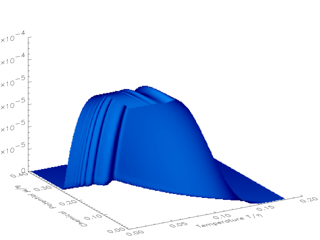
Fig. 3.4: ${\cal B}(\mu,T)$ in Eq. (3.2.21): ${\cal B}(\mu,T)>0$ marks the domain: ${\cal D}$, of confinement and DCSB, with the line ${\cal B}(\mu,T)=0$ demarcating the phase boundary. At $\mu=0$, the transition is second order with mean field critical exponents and $T_{c}=169\,$MeV, using $\eta=1.06\,$GeV. For all nonzero $\mu$ the transition is first order with a tricritical point at $(\mu=0,T_{c})$. At $T=0$, $\mu_{c}=300\,$MeV. The value is $25$% larger; i.e., $\mu_{c}=375\,$MeV, in the model defined by ${\cal D}_{\rm B}$, which improves the ultraviolet behaviour of the effective interaction [197], and in a two-flavour, ultrarelativistic Fermi gas at this chemical potential the baryon number density is $2.9\,\rho_{0}$, $\rho_{0}=0.16\,$fm^-3. (Adapted from Ref. [176].)

The criterion of maximal pressure was also employed in Ref. [198], wherein the model effective interaction saturates in the infrared and exhibits one-loop improved ultraviolet behaviour analogous to that in Eq. (2.2.35). The calculated $\mu=0$ critical temperature agrees with the estimate in Table 3.1 and the $T=0$ critical chemical potential: $\mu_{c}=422\,$MeV, is just $13$% larger than that estimated in Ref. [197]. A similar interaction was employed in Ref. [195], wherein $(\mu=0,T_{c})$ agrees with Table 3.1. However, the estimate of $(\mu_{c},T=0)$ is $60$% larger than in Refs. [197, 198] and is likely too high. The usual range is $\mu_{c}\in[300,400]\,$MeV; e.g., see also Refs. [200, 201].

As clear in Fig. 3.4, the chiral phase boundary traces out a curve in the $(\mu,T)$-plane. In Ref. [198], beginning at $(\mu_{c},T=0)$, this curve describes a line of first order critical points that ends with a tricritical point at $(\mu_{\rm tc}\approx 0.5\,\mu_{c},T_{\rm tc}\approx 0.8\,T_{c})$. For $T>T_{\rm tc}$ the transition is second order. In comparison with the ${\cal D}_{\rm A}$ model, this is a shift of the tricritical point away from the $\mu=0$ axis. We expect such a relocation to be a feature of all models with a better treatment of the ultraviolet behaviour of the effective interaction; e.g., there are preliminary indications that in the separable model of Ref. [194] a tricritical point is located at $(\mu_{\rm tc}\approx 0.4\,\mu_{c},T_{\rm tc}\approx 0.9\,T_{c})$. The existence of a tricritical point has observable consequences [202]. However, if it occurs at a value of $\mu$ as large as that estimated in these models it may be difficult to detect using the relativistic heavy ion collider [RHIC], which will focus on the domain of low baryon number density.

With ${\cal B}(\mu,T)>0$, then, in the exploration of hadronic observables using the rainbow-ladder truncation, $p_{\Sigma_{\rm NG}}(\mu,T)$ describes the free energy of the “vacuum” or “ground state,” relative to which all excitations are measured $\forall\,(\mu,T)\in{\cal D}$; i.e., in the domain of confinement and DCSB. Therefore $p_{\Sigma_{\rm NG}}$ is not directly observable and does not contribute to the thermodynamic pressure. Nevertheless, it does evolve with changes in $(\mu,T)$, as evident in Fig. 3.4, and this evolution simply reflects the $(\mu,T)$-dependence of the dressed-quark self energies, upon which it depends. [NB. If it did not evolve there could never be a phase transition.] The changes in the dressed-quark self energy represent the $(\mu,T)$-dependent rearrangement of the vacuum and are indirectly observable; e.g., in the behaviour of hadron masses and decay constants. Hence, on the domain ${\cal D}$, they are evident in changes of the only true contributions to the pressure; i.e., those of the colour singlet hadronic correlations. At the phase boundary, denoted by $\partial{\cal D}$: $\left.p_{\Sigma_{\rm NG}}(\mu,T)\right|_{\partial{\cal D}}=\left.p_{\Sigma_{\rm W}}(\mu,T)\right|_{\partial{\cal D}}$. This is the last vacuum reference point: hereafter dressed-quarks and -gluons are the active degrees of freedom.

The dressed-quarks’ contribution to the pressure is

$$P_{q}(\mu,T)=\theta({\cal D})\left\{p_{\Sigma_{\rm W}}(\mu,T)-\left.p_{\Sigma_{\rm W}}(\mu,T)\right|_{\partial{\cal D}}\right\},$$ (3.2.23)

where $\theta({\cal D})$ is a step function, equal to one for $(T,\mu)\in{\cal D}$. This pressure can be calculated numerically and is depicted in Fig. 3.5 for model ${\cal D}_{\rm A}$. As evident in Eq. (3.2.18), nonperturbative, momentum-dependent modifications of the dressed-quark’s vector self energy persist into the deconfined domain and this feature retards the approach of the pressure to the ultrarelativistic limit:

$$p_{\rm UR}(\mu,T)=N_{c}N_{f}\frac{1}{12\pi^{2}}\left(\mu^{4}+2\pi^{2}\mu^{2}T^{2}+\mbox{\footnotesize$\frac{7}{15}$}\pi^{4}T^{4}\right)\,.$$ (3.2.24)

A qualitatively similar result is observed in numerical simulations of $T\neq 0$ lattice-QCD [175]. Such a correspondence is impossible in models where the dressed-quark vector self energy is omitted.

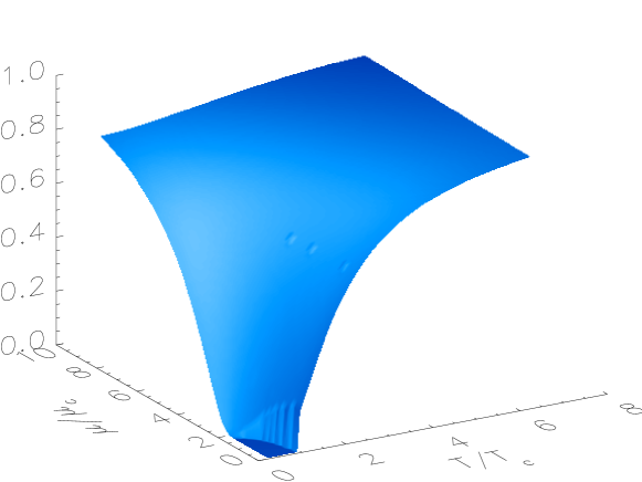
Fig. 3.5: $P_{q}(\mu,T)$ in Eq. (3.2.23) calculated using the ${\cal D}_{\rm A}$ and normalised by the pressure of an ultrarelativistic Fermi gas, Eq. (3.2.24). This ratio approaches one slowly; e.g., at $(\mu=0,T\sim 2\,T_{c})$ or $(\mu\sim 3\,\mu_{c},T=0)$, $P_{q}(\mu,T)$ is only one-half of the free particle pressure. The retardation is a consequence of the persistence into the deconfined domain of nonperturbative effects in the dressed-quark’s vector self energy. Note the “mirroring” of the $T$-dependence in the evolution with $\mu$, which we anticipate is a general feature. (Adapted from Ref. [176].)

The pressure in Eq. (3.2.23) is incomplete. It is zero in the confined domain where, as remarked above, the only contribution is that of colour singlet hadronic correlations. Those contributions can be estimated; e.g., using the hadronisation techniques of Ref. [203], but that has not yet been done. In the deconfined domain, one must add the contribution of the dressed-gluons. However, hitherto the model studies have employed “frozen” gluons; i.e., the structure of the effective interaction does not evolve with $(\mu,T)$. $T\neq 0$ lattice-QCD simulations suggest that to be a good approximation, at least until very near the phase boundary [175], and Ref. [187] indicates that changes in the interaction in this vicinity have little effect on the properties of the transitions. That is good because improving on the frozen approximation is difficult, requiring information about the effective interaction in a new domain. A first step is to allow the mass-scale characterising the infrared behaviour of the interaction to drop suddenly and significantly near the phase boundary, thereby mocking-up the $T$-dependence of the string tension. Such a study is presently lacking.

Not withstanding these weaknesses, the pressure depicted in Fig. 3.5 still provides a rudimentary model for the dressed-quark pressure that exhibits significant new qualitative features; e.g., the persistence into the deconfined domain of nonperturbative effects in the vector self energy yields an EOS much softer than that of a bag model. In this capacity it has been used to explore the structure and stability of nonstrange quark stars [204]. References [176, 197, 205] indicate that a transition to quark matter should occur at approximately three-times nuclear matter density, and the comparison between results obtained with the EOS depicted in Fig. 3.5 and a bag model EOS shows; e.g., that the prediction for the maximum stable radius of a pure quark star is model-independent: $8$–$10\,$km, also in agreement with estimates based on a colour dielectric model [206]. The maximum mass, however, is very sensitive to the EOS. The quark core described by Eq (3.2.23) must be surrounded by an hadronic crust and that will also affect the properties of the star. The problem rapidly becomes involved, and determining the composition of dense astrophysical objects and those signals that point to the realisation of quark matter in their core is an important focus of contemporary research; e.g., Refs. [194, 206, 207, 208].

Superfluidity in Quark Matter       In Sec. 2.3 we described aspects of diquark correlations and the manner in which they help to understand baryon properties. Another aspect follows from the meson-diquark auxiliary-field effective action [147, 148]: the steepest descent approximation to the vacuum pressure suggests the possibility of diquark condensation; i.e., quark-quark Cooper pairing, and that was first explored using a simple version of the Nambu–Jona-Lasinio model [209]. A nonzero chemical potential promotes Cooper pairing in fermion systems and the possibility that it is exhibited in quark matter was considered using the rainbow-ladder truncation of the gap equation [210]. Interest in that possibility has been renewed [211]. A quark-quark Cooper pair is a composite boson with both electric and colour charge, and hence superfluidity in quark matter entails superconductivity and colour superconductivity. However, the last feature makes it difficult to identify an order parameter that can characterise a transition to the superfluid phase: the Cooper pair is gauge dependent and an order parameter is ideally describable by a gauge-invariant operator.

As we saw above, at $\mu=0=T$ QCD exhibits a nonzero quark-antiquark condensate but it is undermined by increasing $\mu$ and $T$, and there is a domain of the $(\mu,T)$-plane, evident in Fig. 3.4, for which $\langle\bar{q}q\rangle=0$. Increasing $T$ also opposes Cooper pairing. However, since increasing $\mu$ promotes it, there may be a (large-$\mu$,low-$T$)-subdomain in which quark matter exists in a superfluid phase. While that domain may not be accessible at RHIC, such conditions might exist in the core of dense astrophysical objects [210], which could undergo a transition to superfluid quark matter as they cool. Unambiguous signals of such a superfluid phase are actively being sought; e.g, Refs. [194, 208].

We take Ref. [151] as our exemplar, in which it was observed that a direct means of determining whether a SU${}_{c}(N$) gauge theory supports $0^{+}$ diquark condensation is to study the gap equation satisfied by

$$\mbox{\boldmath$D$}(p,\mu):={\cal S}(p,\mu)^{-1}=\left(\begin{array}[]{cc}D(p,\mu)&\Delta^{i}(p,\mu)\,\gamma_{5}\lambda_{\wedge}^{i}\\ -\Delta^{i}(p,-\mu)\,\gamma_{5}\lambda_{\wedge}^{i}&CD(-p,\mu)^{\rm t}C^{\dagger}\end{array}\right).$$ (3.2.25)

Here $T=0$, for illustrative simplicity and because temperature can only act to destabilise a Cooper pair, and, with $\omega_{[\mu]}=p_{4}+i\mu$,

$$D(p,\mu)=i\vec{\gamma}\cdot\vec{p}\,A(\vec{p}\,^{2},\omega_{[\mu]}^{2})+B(\vec{p}\,^{2},\omega_{[\mu]}^{2})+i\gamma_{4}\,\omega_{[\mu]}\,C(\vec{p}\,^{2},\omega_{[\mu]}^{2})\,;$$ (3.2.26)

i.e., the inverse of the dressed-quark $2$-point function, Eq. (3.1.11). In Eq. (3.2.25), $\{\lambda_{\wedge}^{i}$, $i=1\ldots n^{\wedge}_{c}$, $n^{\wedge}_{c}=N_{c}(N_{c}-1)/2\}$ are the antisymmetric generators of SU${}_{c}(N_{c})$ and $C$ is the charge conjugation matrix, Eq. (2.3.8). Using such a gap equation to study superfluidity makes unnecessary a truncated bosonisation, which in all but the simplest models is a procedure difficult to improve systematically.

In addition to the usual colour, Dirac and isospin indices carried by the elements of $\mbox{\boldmath$D$}(p,\mu)$, the explicit matrix structure in Eq. (3.2.25) exhibits a quark bispinor index and is made with reference to

$$Q(x):=\left(\begin{array}[]{c}q(x)\\ \underline{q}(x):=\tau^{2}_{f}\,C\,\bar{q}^{\rm t}\end{array}\right)\,,\;\;\bar{Q}(x):=\left(\begin{array}[]{cc}\bar{q}(x)\;\;\bar{\underline{q}}(x):=q^{\rm t}\,C\,\tau^{2}_{f}\end{array}\right),$$ (3.2.27)

where $\{\tau_{f}^{i}:i=1,2,3\}$ are Pauli matrices, Eq. (2.1.7), that act on the isospin index. (Only two-flavour theories are considered in this exemplar. Additional possibilities open in three-flavour theories [212].)

As we have seen, a nonzero quark condensate: $\langle\bar{q}q\rangle\neq 0$, is represented in the solution of the gap equation by $B(\vec{p}\,^{2},\omega_{[\mu]}^{2})\not\equiv 0$. The new but analogous feature here is that diquark condensation is characterised by $\Delta^{i}(p,\mu)\not\equiv 0$, for at least one $i$. That is clear if one considers the quark piece of the QCD Lagrangian density: $L[\bar{q},q]$. It is a scalar and hence $L[\bar{q},q]^{\rm t}=L[\bar{q},q]$. Therefore $L[\bar{q},q]\propto L[\bar{q},q]+L[\bar{q},q]^{\rm t}$, and that sum, and hence the action, can be re-expressed in terms of a diagonal matrix using the bispinor fields in Eq. (3.2.27): $\bar{Q}\,{\rm diag}[D,CD^{\rm t}C^{\dagger}]Q$. It is plain now that a dynamically-generated lower-left element in $\mbox{\boldmath$D$}(p,\mu)$, the inverse of the dressed-bispinor propagator, corresponds to a $\bar{\underline{q}}q$ [diquark] correlation.

The bispinor gap equation can be written in the form

$$\mbox{\boldmath$D$}(p,\mu)=\mbox{\boldmath$D$}_{0}(p,\mu)+\left(\begin{array}[]{cc}\Sigma_{11}(p,\mu)&\Sigma_{12}(p,\mu)\\ \gamma_{4}\,\Sigma_{12}(-p,\mu)\,\gamma_{4}&C\Sigma_{11}(-p,\mu)^{\rm t}C^{\dagger}\end{array}\right),$$ (3.2.28)

where in the absence of a diquark source term

$$\mbox{\boldmath$D$}_{0}(p,\mu)=(i\gamma\cdot p+m)\tau_{Q}^{0}-\mu\,\tau_{Q}^{3}\,,$$ (3.2.29)

with $m$ the current-quark mass, and the additional Pauli matrices: $\{\tau_{Q}^{\alpha},\alpha=0,1,2,3\}$, act on the bispinor indices. The structure of $\Sigma_{ij}(p,\mu)$ specifies the theory and, in practice, also the approximation or truncation of it.

Two colour QCD [QC₂D] provides an important and instructive example. In this case $\Delta^{i}\lambda_{\wedge}^{i}=\Delta\tau^{2}_{c}$ in Eq. (3.2.25), with $\mbox{\footnotesize$\frac{1}{2}$}\vec{\tau_{c}}$ the generators of $SU_{c}(2)$, and it is useful to employ a modified bispinor

$$Q_{2}(x) := \left(\begin{array}[]{c}q(x)\\ \underline{q}_{2}:=\tau^{2}_{c}\,\underline{q}(x)\end{array}\right),\;$$ (3.2.32)

with $\bar{Q}_{2}$ the obvious analogue of $\bar{Q}$ in Eq. (3.2.27). Now the Lagrangian’s fermion-gauge-boson interaction term is simply

$$\bar{Q}_{2}(x)\,\mbox{\footnotesize$\frac{i}{2}$}g\gamma_{\mu}\tau_{c}^{k}\tau_{Q}^{0}\,Q_{2}(x)\,A_{\mu}^{k}(x)$$ (3.2.33)

because SU${}_{c}(2)$ is pseudoreal; i.e., $\tau^{2}_{c}\left(-\vec{\tau}_{c}\right)^{\rm t}\tau^{2}_{c}=\vec{\tau}_{c}\,,\;$ and the fundamental and conjugate representations are equivalent. (That the interaction term takes this form is easily seen using $L[\bar{q},q]^{\rm t}=L[\bar{q},q]$.)

Using the pseudoreality of SU${}_{c}(2)$ it can be shown that, for $\mu=0$ and in the chiral limit, the general solution of the bispinor gap equation is [151]

$$\mbox{\boldmath$D$}(p)=i\gamma\cdot p\,A(p^{2})+{\cal V}(-\mbox{\boldmath$\pi$})\,{\cal M}(p^{2})\,,\;\;{\cal V}(\mbox{\boldmath$\pi$})=\exp\left\{i\gamma_{5}\,\sum_{\ell=1}^{5}\,T^{\ell}\,\pi^{\ell}\right\}={\cal V}(-\mbox{\boldmath$\pi$})^{-1}\,,$$ (3.2.34)

where $\pi^{\ell=1,\ldots,5}$ are arbitrary constants and $\{T^{1,2,3}=\tau_{Q}^{3}\otimes\vec{\tau_{f}},\,T^{4}=\tau_{Q}^{1}\otimes\tau_{f}^{0},\,T^{5}=\tau_{Q}^{2}\otimes\tau_{f}^{0}\}$, $\{T^{i},T^{j}\}=2\delta^{ij}$, so that

$${\cal S}(p)=\frac{-i\gamma\cdot pA(p^{2})+{\cal V}(\mbox{\boldmath$\pi$}){\cal M}(p^{2})}{p^{2}A^{2}(p^{2})+{\cal M}^{2}(p^{2})}\,:=\,-i\gamma\cdot p\,\sigma_{V}(p^{2})+{\cal V}(\mbox{\boldmath$\pi$})\,\sigma_{S}(p^{2})\,.$$ (3.2.35)

[$\mbox{\boldmath$\pi$}=(0,0,0,0,-\mbox{\footnotesize$\frac{1}{4}$}\pi)$ produces an inverse bispinor propagator with the simple form in Eq. (3.2.25).] That the gap equation is satisfied for any constants $\pi^{\ell}$ signals a vacuum degeneracy: if the interaction supports a mass gap, then that gap describes a five-parameter continuum of degenerate condensates:

$$\langle\bar{Q}_{2}{\cal V}(\mbox{\boldmath$\pi$})Q_{2}\rangle\neq 0\,,$$ (3.2.36)

and there are 5 associated Goldstone bosons: 3 pions, a diquark and an anti-diquark. In this construction, Eq. (3.2.34), one has a simple elucidation of a necessary consequence of the Pauli-Gürsey symmetry of QC₂D. For $m\neq 0$, the gap equation requires ${\rm tr}_{FQ}\left[T^{i}{\cal V}\right]=0\,,$ so that in this case only $\langle\bar{Q}_{2}Q_{2}\rangle\neq 0$ and the Goldstone bosons are now massive but remain degenerate.

For $\mu\neq 0$ the general solution of the gap equation has the form

$$\mbox{\boldmath$D$}(p,\mu)=\left(\begin{array}[]{cc}D(p,\mu)&\gamma_{5}\,\Delta(p,\mu)\\ -\gamma_{5}\Delta^{\ast}(p,\mu)&CD(-p,\mu)C^{\dagger}\end{array}\right)\,,$$ (3.2.37)

and in the absence of a diquark condensate; i.e., for $\Delta\equiv 0$,

$$[U_{B}(\alpha),\mbox{\boldmath$D$}(p,\mu)]=0\,,\;U_{B}(\alpha):={\rm e}^{i\alpha\tau_{Q}^{3}\otimes\tau_{f}^{0}}\,,$$ (3.2.38)

which is a manifestation of baryon number conservation in QC₂D. In this case the explicit form of the gap equation is complicated but its features and those of its solutions are easily illustrated using the model ${\cal D}_{\rm A}$ introduced above; e.g., it becomes clear that a chemical potential promotes fermion-pair condensation, at the expense of fermion-antifermion pairs, and $\Delta\in\mbox{$\rule{1.0pt}{6.99997pt}{\rm R}$}$, $\forall\mu$. The rainbow-truncation gap equation was solved using this model in Ref. [151], and the relative stability of the quark- and diquark-condensed phases measured via the pressure difference

$$\delta p(\mu):=p_{\Sigma[B=0,\Delta]}(\mu)-p_{\Sigma[B,\Delta=0]}(\mu)\,,$$ (3.2.39)

where the pressure here is obtained as an obvious generalisation of Eq. (3.1.7). $\delta p(\mu)$ can be expressed in terms of $\mu$-dependent bag constants

$${\cal B}_{B}(\mu):=p_{\Sigma[B,\Delta=0]}(\mu)-p_{\Sigma[B=0,\Delta=0]}(\mu)\,,\;\;{\cal B}_{\Delta}(\mu):=p_{\Sigma[B=0,\Delta]}(\mu)-p_{\Sigma[B=0,\Delta=0]}(\mu)\,,$$ (3.2.40)

which measure the stability of a quark- or diquark-condensed vacuum relative to that with chiral symmetry realised in the Wigner-Weyl mode. [NB. Improving on rainbow-ladder truncation may yield quantitative changes of $\mathrel{\hbox to0.0pt{\lower 4.0pt\hbox{\hskip 0.0pt$\sim$}\hss}\raise 1.0pt\hbox{$<$}}20$% in the exemplary results that follow, however, the pseudoreality of QC₂D and the equal dimension of the colour and bispinor spaces, which underly the theory’s Pauli-Gürsey symmetry, ensure that the entire discussion remains qualitatively unchanged.]

The $(m,\mu)=0$ degeneracy of the quark and diquark condensates, Eq. (3.2.36), is manifest in

$${\cal B}_{B}(0)={\cal B}_{\Delta}(0)=(0.13\,m_{J=1})^{4}\,,$$ (3.2.41)

where $m_{J=1}$ is the $(m,\mu)=0$ mass of the model’s vector meson, calculated in rainbow-ladder truncation. Increasing $\mu$ at $m=0$ and excluding diquark condensation, chiral symmetry is restored at

$$\mu_{2c}^{B,\Delta=0}=0.40\,m_{J=1}\,,$$ (3.2.42)

where ${\cal B}_{B}(\mu)=0$. However, $\forall\mu>0$: $\delta p(\mu)>0$ and ${\cal B}_{\Delta}(\mu)>0\,,$ with

$${\cal B}_{\Delta}(\mu_{2c}^{B,\Delta=0})=(0.20\,m_{J=1})^{4}>{\cal B}_{\Delta}(0).$$ (3.2.43)

Therefore the vacuum is unstable with respect to diquark condensation for all $\mu>0$, and this is always dynamically preferred over quark condensation.

$(B=0,\Delta\neq 0)$ in Eq. (3.2.37) corresponds to $\mbox{\boldmath$\pi$}=(0,0,0,0,\mbox{\footnotesize$\frac{1}{2}$}\pi)$ in Eq. (3.2.36); i.e., $\langle\bar{Q}_{2}i\gamma_{5}\tau_{Q}^{2}Q_{2}\rangle\neq 0$. The usual chiral [$SU_{A}(2)$] transformations are realised via

$$\mbox{\boldmath$D$}(p,\mu)\to V(\vec{\pi})\,\mbox{\boldmath$D$}(p,\mu)\,V(\vec{\pi})\,,\;\;V(\vec{\pi}):={\rm e}^{i\gamma_{5}\vec{\pi}\cdot\vec{T}}\,,\;\vec{\pi}=(\pi^{1},\pi^{2},\pi^{3})\,,$$ (3.2.44)

and therefore, since the anticommutator $\{\vec{T},T^{4,5}\}=0$, a diquark condensate does not break chiral symmetry. However, $(B=0,\Delta\neq 0)$ does yield a dressed-bispinor propagator that violates reflection positivity and hence the model exhibits confinement to arbitrarily large densities. [NB. Reference [151] employs a frozen gluon approximation. In a more realistic analysis, the $\mu$-dependence of $\eta$, the mass-scale characterising the model, would be significant for $\mu\sim\mu_{2c}^{B,\Delta=0}$, and $\eta\to 0$ as $\mu\to\infty$, which would ensure deconfinement at large-$\mu$.] Finally, although the $\mu\neq 0$ theory is invariant under

$$Q_{2}\to U_{B}(\alpha)\,Q_{2}\,,\;\bar{Q}_{2}\to\bar{Q}_{2}\,U_{B}(-\alpha)\,,$$ (3.2.45)

which is associated with baryon number conservation, the diquark condensate breaks this symmetry:

$$\langle\bar{Q}_{2}i\gamma_{5}\tau_{Q}^{2}Q_{2}\rangle\to\cos(2\alpha)\,\langle\bar{Q}_{2}i\gamma_{5}\tau_{Q}^{2}Q_{2}\rangle-\sin(2\alpha)\,\langle\bar{Q}_{2}i\gamma_{5}\tau_{Q}^{1}Q_{2}\rangle\,.$$ (3.2.46)

Hence, for $(m=0,\mu\neq 0)$, one Goldstone mode remains. (These symmetry breaking patterns and the concomitant numbers of Goldstone modes in QC₂D are also described in Ref. [213].)

For $m\neq 0$ and small values of $\mu$, the gap equation only admits a solution with $\Delta\equiv 0$; i.e., diquark condensation is blocked and this is because the current-quark mass is a source of quark condensation. However, with increasing $\mu$ a diquark condensate is generated and the ${\cal D}_{\rm A}$ model exhibits the following minimum chemical potentials for diquark condensation:

$$m=0.013\,m_{J=1}\Rightarrow\mu^{\Delta\neq 0}=0.051\,m_{J=1}\,,\;\;m=0.13\,m_{J=1}\Rightarrow\mu^{\Delta\neq 0}=0.092\,m_{J=1}\,.$$ (3.2.47)

This retardation of diquark condensation by a nonzero current-quark mass can also be seen in Ref. [214].

The exploration of superfluidity in true QCD encounters two differences: the dimension of the colour space is greater than that of the bispinor space and the fundamental and conjugate representations of the gauge group are not equivalent. The latter is of obvious importance because it entails that the quark-quark and quark-antiquark scattering matrices are qualitatively different. As we saw above in connection with Eq. (2.3.42), these differences ensure that colour singlet meson bound states exist but [necessarily coloured] diquark bound states do not.

$n_{c}^{\wedge}=3$ in QCD and hence in canvassing superfluidity it is necessary to choose a direction for the condensate in colour space; e.g., $\Delta^{i}\lambda^{i}_{\wedge}=\Delta\,\lambda^{2}$ in Eq. (3.2.25), so that

$$\mbox{\boldmath$D$}(p,\mu)=\left(\begin{array}[]{c|c}D_{\|}(p,\mu)P_{\|}+D_{\perp}(p,\mu)P_{\perp}&\Delta(p,\mu)\gamma_{5}\lambda^{2}\\ \hline\cr-\Delta(p,-\mu)\gamma_{5}\lambda^{2}\mbox{\rule{0.0pt}{10.00002pt}}&CD_{\|}(-p,\mu)C^{\dagger}P_{\|}+CD_{\perp}(p,\mu)C^{\dagger}P_{\perp}\end{array}\right)\,,$$ (3.2.48)

where $P_{\|}=(\lambda^{2})^{2}$, $P_{\perp}+P_{\|}={\rm diag}({1,1,1})$, and $D_{\|}$, $D_{\perp}$ are defined via obvious generalisations of Eqs. (3.2.25), (3.2.26). (NB. It is this selection of a direction in colour space that opens the possibility for colour-flavour locked diquark condensation in a theory with three effectively-massless quarks; i.e., current-quark masses $\ll\mu$ [215].) In Eq. (3.2.48) the evident, demarcated block structure makes explicit the bispinor index. Here each block is a $3\times 3$ colour matrix and the subscripts: $\|$, $\perp$, indicate whether or not the subspace is accessible via $\lambda_{2}$. The bispinors associated with this representation are given in Eqs. (3.2.27) and in this case the Lagrangian’s quark-gluon interaction term is

$$\bar{Q}(x)ig\Gamma_{\mu}^{a}Q(x)A_{\mu}^{a}(x)\,,\;\;\Gamma_{\mu}^{a} = \left(\begin{array}[]{c|c}\mbox{\footnotesize$\frac{1}{2}$}\gamma_{\mu}\lambda^{a}&0\\[0.0pt] \hline\cr 0\mbox{\rule{0.0pt}{10.00002pt}}&-\mbox{\footnotesize$\frac{1}{2}$}\gamma_{\mu}(\lambda^{a})^{\rm t}\end{array}\right)\,.$$ (3.2.51)

It is straightforward to derive the gap equation at arbitrary order in the truncation scheme of Ref. [108] and it is important to note that because

$$D_{\|}(p,\mu)P_{\|}+D_{\perp}(p,\mu)P_{\perp}=\lambda^{0}\left\{\mbox{\footnotesize$\frac{2}{3}$}D_{\|}(p,\mu)+\mbox{\footnotesize$\frac{1}{3}$}D_{\perp}(p,\mu)\right\}+\mbox{\footnotesize$\frac{1}{\sqrt{3}}$}\lambda^{8}\left\{D_{\|}(p,\mu)-D_{\perp}(p,\mu)\right\}$$ (3.2.52)

the interaction: $\Gamma_{\mu}^{a}{\cal S}(p,\mu)\Gamma_{\nu}^{a}$, necessarily couples the $\|$- and $\perp$-components. That interplay is discarded in models that ignore the vector self energy of quarks, which, as we have repeatedly seen, is a qualitatively important feature of QCD [164, 176, 216, 217].

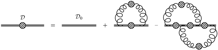
Fig. 3.6: Illustration of the dressed-ladder vertex-corrected gap equation, which is the next-to-leading-order in the truncation scheme of Ref. [108]. [The ladder truncation is obtained by dropping the last diagram.] Each bispinor quark-gluon vertex is bare, given by Eq. (3.2.51), but the shaded circles mark quark and gluon $2$-point functions that are dressed. The corresponding truncation in the relevant Bethe-Salpeter equations ensures the absence of diquark bound states in the strong interaction spectrum. (Adapted from Ref. [151].)

Reference [151] explored the possibility of diquark condensation in QCD via the gap equation using the model defined by ${\cal D}_{\rm A}$ in both the rainbow and a vertex-corrected truncation. The latter is illustrated in Fig. 3.6. For $\mu=0$ the rainbow-ladder truncation yields

$$\begin{array}[]{ccc}m_{\omega}^{2}=m_{\rho}^{2}=\mbox{\footnotesize$\frac{1}{2}$}\,\eta^{2}\,,&\langle\bar{q}q\rangle^{0}=(0.11\,\eta)^{3}\,,&{\cal B}_{B}(\mu=0)=(0.10\,\eta)^{4}\,,\end{array}$$ (3.2.53)

and momentum-dependent vector self energies, Eq. (3.2.14), which lead to an interaction between the $\|$- and $\perp$-components of $D$ that blocks diquark condensation [218]. This is in spite of the fact that $\lambda^{a}\lambda^{2}(-\lambda^{a})^{\rm t}=\mbox{\footnotesize$\frac{1}{2}$}\lambda^{a}\lambda^{a},$ which entails that the rainbow-truncation quark-quark scattering kernel is purely attractive and strong enough to produce diquark bound states [150]. [Remember that in the colour singlet meson channel the rainbow-ladder truncation gives the colour coupling $\lambda^{a}\lambda^{a}$.] For $\mu\neq 0$ and in the absence of diquark condensation, we saw in connection with Fig. (3.4) that the model exhibits coincident, first order chiral symmetry restoring and deconfining transitions at

$$\mu_{c,\,{\rm rainbow}}^{B,\Delta=0}=0.28\,\eta=0.3\,{\rm GeV}\,.$$ (3.2.54)

For $\mu\neq 0$, however, the rainbow-truncation gap equation admits a solution with $\Delta(p,\mu)\not\equiv 0$ and $B(p,\mu)\equiv 0$. $\delta p(\mu)$ in Eq. (3.2.39) again determines whether the stable ground state is the quark-condensed or superfluid phase. With increasing $\mu$, ${\cal B}_{B}(\mu)$ decreases, very slowly at first, and ${\cal B}_{\Delta}(\mu)$ increases rapidly from zero. That evolution continues until

$$\mu_{c,\,{\rm rainbow}}^{B=0,\Delta}=0.25\,\eta=0.89\,\mu_{c,\,{\rm rainbow}}^{B,\Delta=0}\,,$$ (3.2.55)

where ${\cal B}_{\Delta}(\mu)$ becomes greater-than ${\cal B}_{B}(\mu)$. This signals a first order transition to the superfluid ground state and at the boundary

$$\langle\bar{Q}i\gamma_{5}\tau_{Q}^{2}\lambda^{2}Q\rangle_{\mu=\mu_{c,\,{\rm rainbow}}^{B=0,\Delta}}=(0.65)^{3}\,\langle\bar{Q}Q\rangle_{\mu=0}\,.$$ (3.2.56)

The chemical potential at which the switch to the superfluid ground state occurs is consistent with other estimates made using models comparable to the rainbow-truncation class [200, 201, 214, 219], as is the magnitude of the gap at this point [200, 201, 215, 220].

A question that now arises is: how sensitive is this phenomenon to the nature of the quark-quark interaction? As we discussed in connection with Eq. (2.3.42), the inhomogeneous ladder BSE exhibits particle-like singularities in the $0^{+}$ diquark channels and such states do not exist in the strong interaction spectrum. Does diquark condensation persist when a truncation of the gap equation is employed that does not correspond to a BSE whose solutions exhibit diquark bound states? The vertex corrected gap equation depicted in Fig. 3.6 is just such a truncation and it was also studied in Ref. [151].

In this case there is a $\Delta\not\equiv 0$ solution even for $\mu=0$, and using ${\cal D}_{\rm A}$

$$\begin{array}[]{ccc}m_{\rho}^{2}=(1.1)\,\,m_{\rho}^{2\;{\rm ladder}},&\;\langle\bar{Q}Q\rangle=(1.0)^{3}\,\langle\bar{Q}Q\rangle^{\rm rainbow},&\;{\cal B}_{B}=(1.1)^{4}\,{\cal B}_{B}^{\,{\rm rainbow}}\,,\end{array}$$ (3.2.57)

where the rainbow-ladder results are given in Eqs. (3.2.53), and

$$\langle\bar{Q}i\gamma_{5}\tau_{Q}^{2}\lambda^{2}Q\rangle=(0.48)^{3}\,\langle\bar{Q}Q\rangle\,,\;\;{\cal B}_{\Delta}=(0.42)^{4}\,{\cal B}_{B}\,.$$ (3.2.58)

The last result shows, unsurprisingly, that the quark-condensed phase is favoured at $\mu=0$. Precluding diquark condensation, the solution of the vertex-corrected gap equation exhibits coincident, first order chiral symmetry restoring and deconfinement transitions at

$$\mu_{c}^{B,\Delta=0}=0.77\,\mu_{c,\,{\rm rainbow}}^{B,\Delta=0}\,.$$ (3.2.59)

Admitting diquark condensation, however, the $\mu$-dependence of the bag constants again shows there is a transition to the superfluid phase, here at

$$\mu_{c}^{B=0,\Delta}=0.63\,\mu_{c}^{B,\Delta=0}\,,\;{\rm with}\;\langle\bar{Q}i\gamma_{5}\tau_{Q}^{2}\lambda^{2}Q\rangle_{\mu=0.63\,\mu_{c}^{B,\Delta=0}}=(0.51)^{3}\,\langle\bar{Q}Q\rangle_{\mu=0}\,.$$ (3.2.60)

Thus the material step of eliminating diquark bound states leads only to small quantitative changes in the quantities characterising the still extant superfluid phase.

Solving the inhomogeneous BSE for the $0^{+}$ diquark vertex in the quark-condensed phase provides additional insight [151]. At $\mu=0$ and zero total momentum: $P=0$, the additional [confining] contributions to the quark-quark scattering kernel generate an enhancement in the magnitude of the scalar functions in the Bethe-Salpeter amplitude. However, as $P^{2}$ evolves into the timelike region, the contributions become repulsive and block the formation of a diquark bound state. Conversely, increasing $\mu$ at any given timelike-$P^{2}$ yields an enhancement in the magnitude of the scalar functions, and as $\mu\to\mu_{c}^{B,\Delta=0}$ that enhancement becomes large, which suggests the onset of an instability in the quark-condensed vacuum. This “robustness” of scalar diquark condensation is consistent with the observations in Ref. [221]. However, the studies described herein do not obviate the question of whether the diquark condensed phase is stable with-respect-to dinucleon condensation [222], which requires further attention. [NB. As remarked above, the inclusion of temperature undermines a putative diquark condensate and existing studies [200, 214] suggest that it will disappear for $T\mathrel{\hbox to0.0pt{\lower 4.0pt\hbox{\hskip 0.0pt$\sim$}\hss}\raise 1.0pt\hbox{$>$}}60$–$100\,$MeV. However, such temperatures are high relative to that anticipated inside dense astrophysical objects, which may therefore provide an environment for detecting quark matter superfluidity.]

Finally, this discussion illustrates that, in some respects; such as the transition point and magnitude of the gap, the phase diagram of QC₂D is quantitatively similar to that of QCD. That is a useful observation because the simplest superfluid order parameter is gauge invariant in QC₂D, and the fermion determinant is real and positive, which makes tractable the exploration of superfluidity in QC₂D using numerical simulations of the lattice theory [223]. Hence, the results of those studies may provide an additional, reliable guide to the nature of quark matter superfluidity.

4 Density, Temperature and Hadrons

4.1 Masses and Widths

Temperature       Hitherto we have canvassed the bulk thermodynamic properties of QCD at nonzero $(\mu,T)$. However, the terrestrial formation of a QGP will be signalled by changes in the observable properties of those colour singlet mesons that reach detectors. In this connection, a primary feature of the QGP is chiral symmetry restoration and, since the properties of the pion (mass, decay constant, other vertex residues, etc.) are tied to the dynamical breaking of chiral symmetry, an elucidation of the $T$-dependence of these properties is important; particularly since a prodigious number of pions is produced in heavy ion collisions. Also important is understanding the $T$-dependence of the properties of the scalar analogues and chiral partners of the pion in the strong interaction spectrum. For example, should the mass of a putative light isoscalar-scalar meson [117, 118, 119, 224] fall below $2\,m_{\pi}$, the strong decay into a two pion final state can no longer provide its dominant decay mode. In this case electroweak processes will be the only open decay channels below $T_{c}$ and the state will appear as a narrow resonance [202]. Analogous statements are true of isovector-scalar mesons.

The effective interaction denoted above as ${\cal D}_{\rm C}$ in Eq. (3.2.2), with $\omega=1.2\,m_{t}$, has been employed [121] in an exploration of the $T$-dependence of scalar and pseudoscalar meson properties. As we saw in Sec. 2.3, mesons appear as simple poles in $3$-point vertices and these vertices alone provide information about the persistence of correlations away from the bound state pole, which can be useful in studying the $T$-evolution of a system with deconfinement. For $T\neq 0$ and two flavours, the ladder-truncation of the inhomogeneous BSE for the isovector $0^{-+}$ vertex is

$$\Gamma_{\rm ps}^{i}(p_{\omega_{k}};P_{0};\zeta)=Z_{4}\,\mbox{\footnotesize$\frac{1}{2}$}\tau^{i}\gamma_{5}-\int_{l,q}^{\bar{\Lambda}}\,\mbox{\footnotesize$\frac{4}{3}$}\,g^{2}D_{\mu\nu}(p_{\omega_{k}}-q_{\omega_{l}})\gamma_{\mu}S(q_{\omega_{l}}^{+})\,\Gamma_{\rm ps}^{i}(q_{\omega_{l}};P_{0};\zeta)\,S(q_{\omega_{l}}^{-})\,\gamma_{\nu}\,,$$ (4.1.1)

where $q_{\omega_{l}}^{\pm}=q_{\omega_{l}}\pm P_{0}/2$, and with $P_{0}=(\vec{P},0)$ this is the equation for the zeroth Matsubara mode. [This is an extension of Eq. (2.3.4). Remember, $m_{R}(\zeta)\,\Gamma_{\rm ps}^{i}(p_{\omega_{k}};P_{\Omega_{n}};\zeta)$ is renormalisation point independent.]

The solution of Eq. (4.1.1) has the form [hereafter the $\zeta$-dependence is often implicit]

$$\Gamma_{\rm ps}^{i}(p_{\omega_{k}};\vec{P})=$$

$$\mbox{\footnotesize$\frac{1}{2}$}\tau^{i}\gamma_{5}\,\left[iE_{\rm ps}(p_{\omega_{k}};\vec{P})+\vec{\gamma}\cdot\vec{P}\,F_{\rm ps}(p_{\omega_{k}};\vec{P})+\vec{\gamma}\cdot\vec{p}\,\vec{p}\cdot\vec{P}\,G^{\|}_{\rm ps}(p_{\omega_{k}};\vec{P})+\gamma_{4}\omega_{k}\,\,\vec{p}\cdot\vec{P}\,G^{\perp}_{\rm ps}(p_{\omega_{k}};\vec{P})\right]\,,$$

where the $T\neq 0$ analogues of the $\sigma_{\mu\nu}$-like contributions in Eq. (2.3.9) are omitted because they play a negligible role at $T=0$ [20]. The breaking of $O(4)$ symmetry is responsible for making this $T\neq 0$ amplitude more complicated than its zero-temperature counterpart. For the higher Matsubara frequencies the form is still more complicated, with three additional terms. The scalar functions in Eq. (4.1) exhibit a simple pole at $\vec{P}^{2}+m_{\pi}^{2}=0$ so that

$$\Gamma_{\rm ps}^{i}(p_{\omega_{k}};\vec{P})=\frac{r_{\pi}(\zeta)}{\vec{P}^{2}+m_{\pi}^{2}}\,\Gamma_{\pi}^{i}(p_{\omega_{k}};\vec{P})+{\rm regular,}$$ (4.1.3)

where again regular means terms regular at this pole and $\Gamma_{\pi}^{i}(p_{\omega_{k}};\vec{P})$ is the bound state pion Bethe-Salpeter amplitude, canonically normalised via the obvious $T\neq 0$ extension of Eq. (2.3.6).

The pole position in Eq. (4.1.3) determines the spatial “screening-mass” of the pion’s zeroth Matsubara mode and its inverse describes the persistence length of that mode at equilibrium in the heat bath. There is a screening mass and amplitude for each mode, and each mode’s amplitude is canonically normalised. The full $T\neq 0$ bound state propagator can be calculated via any polarisation tensor that receives a contribution from the bound state but only once all the screening masses have been determined. (For the pion: the pseudoscalar or pseudovector polarisations will serve [42].) The propagator so obtained is defined only on a discrete set of points along what might be called the imaginary-energy axis and the “pole-mass;” i.e., the mass that yields the bound state energy pole for $\vec{p}\sim 0$, is obtained only after an analytic continuation of the propagator onto the real-energy axis. [The loss of $O(4)$ invariance for $T\neq 0$ means that, in general, the pole mass and screening masses are unequal.] That continuation is not unique but an unambiguous result is obtained by requiring that it yield a function that is bounded at complex-infinity and analytic off the real axis [225]. From this description it is nonetheless clear that the screening masses completely specify the properties of $T\neq 0$ bound states. Furthermore, the often used calculational expedient of replacing the meson Matsubara frequencies by a continuous variable: $\Omega_{n}\to-i\nu$, and the identification of the energy scale thus obtained with a pole mass, is seen to be merely an artefice. However, since this prescription yields the correct result for free particle propagators, it might provide an illustrative guide.

The residue in Eq. (4.1.3) is

$$\delta^{ij}\,ir_{\pi}=\,Z_{4}\,{\rm tr}\int_{l,q}^{\bar{\Lambda}}\,\mbox{\footnotesize$\frac{1}{2}$}\tau^{i}\,\gamma_{5}\chi_{\pi}^{j}(q_{\omega_{l}};\vec{P})\,,$$ (4.1.4)

where $\chi_{\pi}(q_{\omega_{l}};\vec{P}):=S(q_{\omega_{l}}^{+})\Gamma_{\pi}(q_{\omega_{l}};\vec{P})S(q_{\omega_{l}}^{-})$ is the unamputated Bethe-Salpeter wave function. [Ref. [121] employs the $f_{\pi}=92\,$MeV normalisation, cf. Eq. (2.3.22)] Substituting Eq. (4.1.3) into Eq. (4.1.1) and equating pole residues yields the homogeneous pion BSE, which provides the simplest way to obtain the bound state amplitude. As already noted, the pion also appears as a pole in the axial-vector vertex and there the residue is the leptonic decay constant

$$\delta^{ij}\,\vec{P}\,f_{\pi}=Z_{2}^{A}\,{\rm tr}\int_{l,q}^{\bar{\Lambda}}\,\mbox{\footnotesize$\frac{1}{2}$}\tau^{i}\,\gamma_{5}\vec{\gamma}\,\chi_{\pi}^{j}(q_{\omega_{l}};\vec{P})\,.$$ (4.1.5)

At $T=0$ in this ${\cal D}_{\rm C}$ model the calculated chiral limit values are [remember: $f_{\pi}=92\,$MeV normalisation]

$$\begin{array}[]{ccc}f_{\pi}^{0}=0.088\,{\rm GeV}\,,&\;-\langle\bar{q}q\rangle^{0}_{1\,{\rm GeV}^{2}}=(0.235\,{\rm GeV})^{3}\,,&\;r_{\pi}^{0}(1\,{\rm GeV}^{2})=(0.457\,{\rm GeV})^{2}\,.\end{array}$$ (4.1.6)

The analogue of Eq. (4.1.1) for the $0^{++}$ vertex is

$$\Gamma_{\rm s}^{\alpha}(p_{\omega_{k}};P_{0};\zeta)=Z_{4}\,\mbox{\footnotesize$\frac{1}{2}$}\tau^{\alpha}\mbox{\large\boldmath$1$}-\int_{l,q}^{\bar{\Lambda}}\,\mbox{\footnotesize$\frac{4}{3}$}\,g^{2}D_{\mu\nu}(p_{\omega_{k}}-q_{\omega_{l}})\gamma_{\mu}S(q_{\omega_{l}}^{+})\,\Gamma_{\rm s}^{i}(q_{\omega_{l}};P_{\Omega_{n}};\zeta)\,S(q_{\omega_{l}}^{-})\,\gamma_{\nu}\,,$$ (4.1.7)

where $\alpha=0,1,2,3$. However, as discussed in connection with Eq. (2.3.23), the combination of rainbow and ladder truncations is not certain to provide a reliable approximation in the scalar sector. Nevertheless, in the absence of an improved, phenomenologically efficacious kernel, Ref. [121] employed Eq. (4.1.7) in the expectation that it would provide some qualitatively reliable insight, an approach justified a posteriori.

The solution of Eq. (4.1.7) has the form

$$\Gamma_{\rm s}^{i}(p_{\omega_{k}};\vec{P})=$$

$$\mbox{\footnotesize$\frac{1}{2}$}\tau^{\alpha}\,\mbox{\large\boldmath$1$}\,\left[E_{\rm s}(p_{\omega_{k}};\vec{P})+i\vec{\gamma}\cdot\vec{p}\,G^{\|}_{\rm s}(p_{\omega_{k}};\vec{P})+i\gamma_{4}\omega_{k}\,G^{\perp}_{\rm s}(p_{\omega_{k}};\vec{P})+i\vec{\gamma}\cdot\vec{P}\,\vec{p}\cdot\vec{P}\,F_{\rm s}(p_{\omega_{k}};\vec{P})\right]\,,$$

where here the requirement that the neutral mesons be charge conjugation eigenstates shifts the $\vec{p}\cdot\vec{P}$ term cf. the $0^{-\,+}$ amplitude in Eq. (4.1). As already observed in connection with Eq. (2.3.69), the scalar functions in Eq. (4.1) exhibit a simple pole at $\vec{P}^{2}+m_{\sigma}^{2}=0$ with residue

$$\delta^{\alpha\beta}\,r_{\sigma}=Z_{4}\,{\rm tr}\int_{l,q}^{\bar{\Lambda}}\,\mbox{\footnotesize$\frac{1}{2}$}\tau^{\alpha}\,\chi_{\sigma}^{\beta}(q_{\omega_{l}};\vec{P})\,.$$ (4.1.9)

However, since a $V-A$ current cannot connect a $0^{++}$ state to the vacuum, the scalar meson does not appear as a pole in the vector vertex; i.e,

$$\delta^{\alpha\beta}\,\vec{P}\,f_{\sigma}=Z_{2}^{A}\,{\rm tr}\int_{l,q}^{\bar{\Lambda}}\,\mbox{\footnotesize$\frac{1}{2}$}\tau^{\alpha}\,\vec{\gamma}\,\chi_{\sigma}^{\beta}(q_{\omega_{l}};\vec{P})\equiv 0\,.$$ (4.1.10)

The homogeneous equation for the scalar bound state amplitude is obtained, as usual, from Eq. (4.1.7) by equating pole residues.

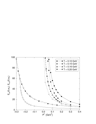
Fig. 4.1: Leading Dirac amplitude for the pseudoscalar (shaded symbols) and scalar (open symbols) vertices [$E$ in Eqs. (4.1), (4.1)] evaluated at $(\vec{p}=0,\omega_{0})$ and plotted as function of $\vec{P}^{2}$ in the chiral limit; i.e., $E(\vec{p}=0,\omega_{0};\vec{P}^{2})$, for a range of temperature values. The bound state poles are evident in each case. (Adapted from Ref. [121].)

The $T$-dependence of the pole positions in the solution of the inhomogeneous BSEs is illustrated in Fig. 4.1, from which it is evident that: 1) at the critical temperature, $T_{c}=152\,$MeV in Table 3.1, one has degenerate, massless pseudoscalar and scalar bound states; and 2) the bound states persist above $T_{c}$, becoming increasingly massive with increasing $T$. These features are also observed in numerical simulations of lattice-QCD [175]. The bound state amplitudes are obtained from the homogeneous BSEs. Above $T_{c}$, all but the leading Dirac amplitudes: $E_{\pi}$, $E_{\sigma}$, vanish and the surviving amplitudes are pointwise identical. These results indicate that the chiral partners are locally identical above $T_{c}$, they do not just have the same mass.

The results are easily understood algebraically. The BSE is a set of coupled homogeneous equations for the Dirac amplitudes. Below $T_{c}$ each of the equations for the subleading Dirac amplitudes has an “inhomogeneity” whose magnitude is determined by $B_{0}$, the scalar piece of the quark self energy, which is dynamically generated in the chiral limit. $B_{0}$ vanishes above $T_{c}$ eliminating the inhomogeneity and allowing a trivial, identically zero solution for each of these amplitudes. Additionally, with $B_{0}\equiv 0$ the kernels in the equations for the dominant pseudoscalar and scalar amplitudes are identical, and hence so are the solutions. It follows from these observations that the Goldberger-Treiman-like relation [42]

$$f_{\pi}^{0}E_{\pi}(p_{\omega_{k}};0)=B_{0}(p_{\omega_{k}})$$ (4.1.11)

is satisfied for all $T$ only because both $f_{\pi}^{0}$ and $B_{0}(p_{\omega_{k}})$ are equivalent order parameters for chiral symmetry restoration.

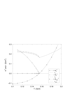
Fig. 4.2: $\hat{m}=0$ results. Left Panel: $T$-dependence of the meson masses-squared and pole-residue matrix elements, Eqs. (4.1.4), (4.1.9), along with the mass-squared: $m_{\rm sym}^{2}$, and residue: $r_{\rm sym}$, calculated in the chirally symmetric $B_{0}\equiv 0$ phase. For $T\leq T_{c}$, $m_{\rm sym}^{2}<0$, which is a signal of the instability of the chirally symmetric phase at low $T$. For $T>T_{c}$, $m_{\pi}^{2}=m_{\sigma}^{2}=m_{\rm sym}^{2}$. Right Panel: $T$-dependence of the masses and pion decay constant, Eq. (4.1.5). $m_{\pi}=0$ within numerical error. (Adapted from Ref. [121]).

Using the calculated bound state amplitudes and dressed-quark propagators, the $T$-dependence of the matrix elements in Eqs. (4.1.4), (4.1.5), (4.1.9) follows. It is depicted in Fig. 4.2 for the chiral limit. Below $T_{c}$ the scalar meson residue in the scalar vertex, $r_{\sigma}$ in Eq. (4.1.9), is a little larger than the residue of the pseudoscalar meson in the pseudoscalar vertex, $r_{\pi}$ in Eq. (4.1.4). However, they are nonzero and equal above $T_{c}$, which is an algebraic consequence of $B_{0}\equiv 0$ and the vanishing of the subleading Dirac amplitudes. As a bona fide order parameter for chiral symmetry restoration

$$f_{\pi}^{0}\propto\sqrt{-t}\,,\;t=(T/T_{c}-1)\mathrel{\hbox to0.0pt{\lower 4.0pt\hbox{\hskip 0.0pt$\sim$}\hss}\raise 1.0pt\hbox{$<$}}0\,,$$ (4.1.12)

as anticipated from the discussion accompanying Table 3.1. The same result was obtained in Ref. [187], where it was observed too that

$$\frac{1}{(r_{\pi}^{0})_{\rm em}}\propto f_{\pi}^{0}\,;$$ (4.1.13)

i.e., the pion charge radius diverges at $T_{c}$ in the chiral limit. This is plausible but Ref. [121] did not attempt its verification. Reference [121] did confirm the behaviour of the ratio of pole residues observed in Ref. [186]:

$$\frac{r_{\pi}^{0}(\zeta)}{f_{\pi}^{0}}\propto\frac{1}{\sqrt{-t}}\,,\;t\mathrel{\hbox to0.0pt{\lower 4.0pt\hbox{\hskip 0.0pt$\sim$}\hss}\raise 1.0pt\hbox{$<$}}0\,.$$ (4.1.14)

The concomitant results: $f_{\pi}^{0}=0$ and $r_{\pi}^{0}\neq 0$ for $t>0$, demonstrate that the pion disappears as a pole in the axial-vector vertex [181] but persists as a pole in the pseudoscalar vertex. Evident also in Fig. 4.2 is that

$$m_{\sigma}^{0}\propto\sqrt{-t}\,,\;\;t\mathrel{\hbox to0.0pt{\lower 4.0pt\hbox{\hskip 0.0pt$\sim$}\hss}\raise 1.0pt\hbox{$<$}}0:$$ (4.1.15)

$m_{\sigma}^{2}$ follows a linear trajectory for $t\mathrel{\hbox to0.0pt{\lower 4.0pt\hbox{\hskip 0.0pt$\sim$}\hss}\raise 1.0pt\hbox{$<$}}0$. Such behaviour in the isoscalar-scalar channel might be anticipated because this channel has vacuum quantum numbers and hence the bound state is a strong interaction analogue of the electroweak Higgs boson [119].

$m_{\rm sym}^{2}$ in Fig. 4.2 is the mass obtained when the chirally symmetric solution of the quark DSE is used in the BSE. [$B_{0}\equiv 0$ is always a solution in the chiral limit.] For $t>0$, $m_{\rm sym}^{2}(T)$ is the unique meson mass-squared trajectory. However, for $t<0$, $m_{\rm sym}^{2}<0$; i.e., the solution of the BSE in the Wigner-Weyl phase exhibits a tachyonic solution. [cf. The Nambu-Goldstone phase masses: $m_{\sigma}^{2}>m_{\pi}^{2}=0$.] By analogy with the $\sigma$-model, this tachyonic mass indicates the instability of the Wigner-Weyl phase below $T_{c}$ and translates into the statement that the pressure is not maximal in this phase. Figure 4.3 depicts the evolution of this [common] meson mass at large $T$. As expected in a gas of weakly interacting quarks and gluons

$$\frac{m_{0^{\pm}{\rm meson}}}{2\,\omega_{0}}\to 1^{-}\,,$$ (4.1.16)

where $\omega_{0}=\pi T$ is a quark’s zeroth Matsubara frequency and “screening mass.” Similar behaviour is observed for the $\rho$-meson mass in Ref. [226] and can be demonstrated algebraically using the ${\cal D}_{\rm A}$ model for the effective interaction [227].

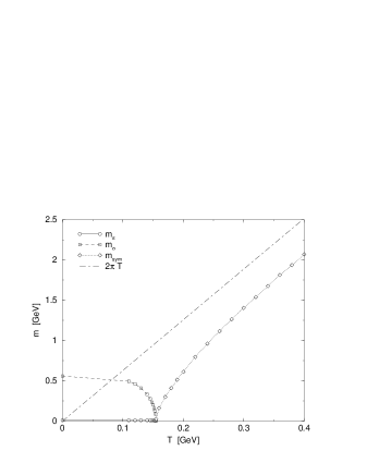
Fig. 4.3: $T$-dependence of the meson masses for large $T$ with $\hat{m}=0$, see Fig. 4.2. $m_{\pi}=m_{\sigma}$ for $T>T_{c}$ and $m/(2\pi T)\to 1^{-}$. This behaviour persists with $\hat{m}\neq 0$, as illustrated in Refs. [194, 226], and observed in lattice-QCD simulations [175].) (Adapted from Ref. [121].)

The results described hitherto were all calculated in the chiral limit. The extension to $\hat{m}\neq 0$ is straightforward although calculations with the renormalisation group improved rainbow-ladder truncation become more time consuming. That is why simpler models, such as employed in Refs. [194, 226], can be useful. For $\hat{m}\neq 0$, chiral symmetry restoration with increasing $T$ is exhibited as a crossover rather than a phase transition. The solutions of the inhomogeneous BSEs again exhibit a pole for all $T$, with the bound state amplitudes obtained from the associated homogeneous equations. In this case the scalar and pseudoscalar bound states are locally identical for $T\mathrel{\hbox to0.0pt{\lower 4.0pt\hbox{\hskip 0.0pt$\sim$}\hss}\raise 1.0pt\hbox{$>$}}\mbox{\footnotesize$\frac{4}{3}$}T_{c}$. Figure 4.4 is the $\hat{m}\neq 0$ analogue of Fig. 4.2. An important result is that the axial-vector Ward-Takahashi identity is satisfied, both above and below the chiral transition temperature, which was demonstrated in Ref. [121] via Eq. (2.3.21): the two sides remain equal $\forall\,T$. The Gell-Mann–Oakes-Renner formula, however, which involves $r_{\pi}^{0}(\zeta)$, fails for $t>-0.1$, as observed too in the separable model study of Ref. [228].

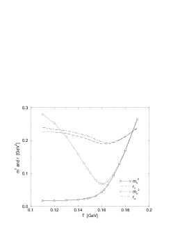
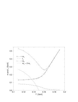
Fig. 4.4: $T$-dependence of the meson masses and pole-residue matrix elements, Eqs. (4.1.4,4.1.5,4.1.9), for $\hat{m}\neq 0$. That the transition has become a crossover is evident in the behaviour of $f_{\pi}$. The meson masses become indistinguishable at $T\sim 1.2\,T_{c}$, a little before the local equivalence is manifest, which is unsurprising given that the mass is an integrated quantity. The small difference between $r_{\sigma}$ and $r_{\pi}$ below $T_{c}$ is again evident and they assume a common value at the same temperature as the masses. (Adapted from Ref. [121].)

As one can anticipate from Sec. 2.3, the calculated $\sigma$ and $\pi$ bound state amplitudes and dressed-quark propagator also make possible a study of two-body decays. For example, the impulse approximation to the isoscalar-scalar-$\pi\pi$ coupling is described by the matrix element

$$g_{\sigma\pi\pi}:=\langle\pi(\vec{p_{1}})\pi(\vec{p_{2}})|\sigma(\vec{p})\rangle$$

$$=2N_{c}{\rm tr}_{D}\int_{l,q}^{\bar{\Lambda}}\,\Gamma_{\sigma}(k_{\omega_{l}};\vec{p})\,S_{u}(k_{++})\,i\Gamma_{\pi}(k_{0+};-\vec{p_{1}})\,S_{u}(k_{+-})\,i\Gamma_{\pi}(k_{-0};-\vec{p_{2}})\,S_{u}(k_{--})\,,$$

$k_{\alpha\beta}=k_{\omega_{l}}+(\alpha/2)\vec{p_{1}}+(\beta/2)\vec{p_{2}}$, in terms of which the width is

$$\Gamma_{\sigma\to(\pi\pi)}=\mbox{\footnotesize$\frac{3}{2}$}\,g_{\sigma\pi\pi}^{2}\,\frac{\sqrt{1-4m_{\pi}^{2}/m_{\sigma}^{2}}}{16\,\pi\,m_{\sigma}}\,.$$ (4.1.18)

The coupling and width obtained from Eq. (4.1) are depicted in Fig. 4.5, which indicates that both vanish at $T_{c}$ in the chiral limit. Again this can be traced to $B_{0}\to 0$. For $\hat{m}\neq 0$, the coupling reflects the crossover but that is not observable because the width vanishes just below $T_{c}$ where the isoscalar-scalar meson mass falls below $2m_{\pi}$ and the phase space factor vanishes. [See the right panel of Fig. 4.4.] The evolution $m_{\sigma}\to 2m_{\pi}$ may, however, be observable via an enhancement in the $\pi\pi\to\gamma\gamma$ cross-section [229].

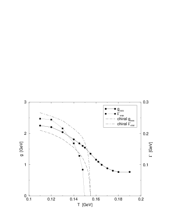
Fig. 4.5: $T$-dependence of the isoscalar-scalar-$\pi\pi$ coupling and width, both in the chiral limit and for realistic light current-quark masses. The phase space factor $(1-(2m_{\pi}/m_{\sigma})^{2})^{1/2}$ is $\theta(T_{c}-T)$ in the chiral limit but nontrivial for $\hat{m}\neq 0$, vanishing at $T\approx 0.98\,T_{c}$; i.e., this decay channel closes at a temperature just $2$% less-than $T_{c}$. (Adapted from Ref. [121].)

Additionally, the particular properties of the $\pi^{0}\to\gamma\gamma$ decay, which is mediated by the “triangle anomaly,” [see the paragraph after Eq. (2.3.41) on page 2.3] make interesting the behaviour of this process at $T\neq 0$. At $T=0$, the anomalous contribution to the divergence of the axial-vector vertex is saturated by the pseudoscalar piece, $E_{\pi}$, of the pion Bethe-Salpeter amplitude [82]

$$\hat{T}_{\mu\nu}(k_{1},k_{2})={\rm tr}\int_{l,q}^{\bar{\Lambda}}\,S(q_{1})\,\gamma_{5}\tau^{3}iE_{\pi}(\hat{q};-P)\,S(q_{2})\,iQ_{e}\Gamma_{\mu}(q_{2},q_{12})\,S(q_{12})\,iQ_{e}\Gamma_{\nu}(q_{12},q_{1})\,,$$ (4.1.19)

where here, just to be specific, $k_{1}=(\vec{k}_{1},0)$, $k_{2}=(\vec{k}_{2},0)$, $P=k_{1}+k_{2}$, $q_{1}=q_{\omega_{l}}-k_{1}$, $q_{2}=q_{\omega_{l}}+k_{2}$, $\hat{q}=\mbox{\footnotesize$\frac{1}{2}$}(q_{1}+q_{2})$, $q_{12}=q_{\omega_{l}}-k_{1}+k_{2}$. Equation (4.1.19) involves the dressed-quark-photon vertex: $\Gamma_{\mu}$, which also appeared in the calculation of $F_{\pi}(Q^{2})$, described in Sec. 2.3. As we saw, quantitatively reliable numerical solutions of the $T=0$ vector vertex equation are now available [107]. However, this anomalous coupling is insensitive to details and an accurate result requires only that the dressed vertex satisfy the vector Ward-Takahashi identity. For $T=0$ with real photons, Eq. (4.1.19) is expressed in terms of one scalar function:

$$\hat{T}_{\mu\nu}(k_{1},k_{2})=\frac{\alpha_{\rm em}}{\pi}\,\epsilon_{\mu\nu\rho\sigma}\,k_{1\rho}\,k_{2\sigma}\,{\cal T}(0)\,.$$ (4.1.20)

Now, as long as $\Gamma_{\mu}$ satisfies the Ward-Takahashi identity, Eq. (2.3.26), one finds algebraically in the chiral limit

$$f_{\pi}^{0}\,{\cal T}(0):=g_{\pi^{0}\gamma\gamma}=1/2\,,$$ (4.1.21)

completely independent of model details [82, 130, 144], as required since at $T=0$ the anomalies are a feature of the global aspects of DCSB [143]. This value reproduces the experimental width. [Remember, the normalisation in this subsection yields $f_{\pi}=92\,$MeV.]

The $T\neq 0$ calculation requires only a valid extension of Eq. (2.3.31) and one such is

$$i\vec{\Gamma}(q_{\omega_{l_{1}}},q_{\omega_{l_{2}}}) = \Sigma_{A}(q_{\omega_{l_{1}}}^{2},q_{\omega_{l_{2}}}^{2})\,i\vec{\gamma}+(\vec{q}_{1}+\vec{q}_{2})\,[\mbox{\footnotesize$\frac{1}{2}$}\,iG(q_{\omega_{l_{1}}},q_{\omega_{l_{2}}})+\Delta_{B}(q_{\omega_{l_{1}}}^{2},q_{\omega_{l_{2}}}^{2})],$$ (4.1.22)

$$i\Gamma_{4}(q_{\omega_{l_{1}}},q_{\omega_{l_{2}}}) = \Sigma_{C}(q_{\omega_{l_{1}}}^{2},q_{\omega_{l_{2}}}^{2})\,i\gamma_{4}+(\omega_{l_{1}}+\omega_{l_{2}})\,[\mbox{\footnotesize$\frac{1}{2}$}\,iG(q_{\omega_{l_{1}}},q_{\omega_{l_{2}}})+\Delta_{B}(q_{\omega_{l_{1}}}^{2},q_{\omega_{l_{2}}}^{2})],$$ (4.1.23)

$$G(q_{\omega_{l_{1}}},q_{\omega_{l_{2}}}) = \vec{\gamma}\cdot(\vec{q}_{1}+\vec{q}_{2})\Delta_{A}(q_{\omega_{l_{1}}}^{2},q_{\omega_{l_{2}}}^{2})+\gamma_{4}(\omega_{l_{1}}+\omega_{l_{2}})\Delta_{C}(q_{\omega_{l_{1}}}^{2},q_{\omega_{l_{2}}}^{2}).$$ (4.1.24)

It is a particular case of the Ansatz in Ref. [230] and satisfies the $T\neq 0$ vector Ward-Takahashi identity

$$(q_{\omega_{l_{1}}}-q_{\omega_{l_{2}}})_{\mu}\,i\Gamma_{\mu}(q_{\omega_{l_{1}}},q_{\omega_{l_{2}}})=S^{-1}(q_{\omega_{l_{1}}})-S^{-1}(q_{\omega_{l_{2}}}).$$ (4.1.25)

For $T\neq 0$ the tensor structure of Eq. (4.1.20) survives to the extent that, with $k_{1}$, $k_{2}$ as defined, it ensures one of the photons is longitudinal (a plasmon) and the other transverse, with

$$\hat{T}_{i4}(k_{1},k_{2})=\frac{\alpha_{\rm em}}{\pi}\,(\vec{k_{1}}\times\vec{k_{2}})_{i}\,{\cal T}(0)\,.$$ (4.1.26)

The $T$-dependence of the anomalous coupling follows from that of ${\cal T}(0)$, and it and the $T$-dependence of the width are depicted in Fig. 4.6. In the chiral limit the interesting quantity is: ${\cal T}(0)=g^{0}_{\pi^{0}\gamma\gamma}/f_{\pi}^{0}$, and obvious in the figure is that it vanishes at $T_{c}$. (It vanishes with a mean field critical exponent [121].) Thus, in the chiral limit, the coupling to the dominant decay channel closes for both charged and neutral pions. These features were anticipated in Ref. [231]. Further, the calculated ${\cal T}(0)$ is monotonically decreasing with $T$, supporting the perturbative O($T^{2}/f_{\pi}^{2})$ analysis in Ref. [232]. For $\hat{m}\neq 0$ both the coupling: $g_{\pi^{0}\gamma\gamma}/f_{\pi}$, and the width exhibit the crossover, with a slight enhancement in the width as $T\to T_{c}$ due to the increase in $m_{\pi}$. This is similar to the results of Ref. [233], although the $T$-dependence depicted here is much weaker because the pion mass approaches twice the $T\neq 0$ free-quark screening-mass from below, never reaching it, Eq. (4.1.16); i.e., the continuum threshold is not crossed.

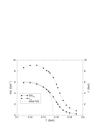
Fig. 4.6: $T$-dependence of the coupling ${\cal T}(0)$ in Eq. (4.1.26) and the $\pi^{0}\to\gamma\gamma$ width: $\Gamma_{\pi\to\gamma\gamma}=\alpha_{\rm em}^{2}m_{\pi}^{3}|{\cal T}(0)|^{2}/(16\pi^{3})$, which is identically zero in the chiral limit because $m_{\pi}=0$. (Adapted from Ref. [121].)

The $T$-dependence of meson properties illustrated here is robust: it agrees with the results obtained in lattice simulations when there is an overlap, and with the results of other models. The local equivalence exhibited by isovector chiral partners above $T_{c}$ might be expected as a general feature of the bound state spectrum in the Wigner-Weyl phase. However, an explicit demonstration is numerically challenging; e.g., in the $\rho$-$a_{1}$ complex the bound state amplitudes have eight independent functions even at $T=0$, compared with the four in the pseudoscalar and scalar amplitudes at $T\neq 0$.

Adding a third light quark introduces one qualitatively new aspect: the $\eta$-$\eta^{\prime}$ system and the restoration of $U_{A}(1)$ symmetry, which can affect the order of the chiral transition [183]. As already observed, it is necessary to move beyond the rainbow-ladder truncation before that can be addressed using the DSEs. The question has been explored in lattice simulations but the results are not currently conclusive: the mass splittings used to characterise the symmetry breaking might become smaller near $T_{c}$ [234] but strong, topological arguments can nevertheless be made in favour of the non-restoration of $U_{A}(1)$ symmetry [235]. Much remains to be done and improved models can be useful.

Chemical Potential       The relation between chemical potential and baryon number density can only be determined after the EOS is known; i.e., via Eq. (3.1.5). As described in connection with Eq. (3.2.23) on page 3.2.23, the dressed-quarks and -gluons contribute nothing to the EOS in the confined domain, even though they dominate it in the QGP, and the only true contributions to the pressure in the confined domain are those of colour singlet bound states. This physical requirement is overlooked in many model explorations of the density dependence of meson properties. For example, in applications of the Nambu–Jona-Lasinio model the EOS for a free fermion gas is used to define a baryon number density. While this is the EOS for that non-confining model it is not a good model for QCD’s EOS.

The application of DSEs in calculating the $\mu$-dependence of hadron properties is rudimentary. However, even that is significant given the problem is currently inaccessible in lattice simulations. The model obtained with ${\cal D}_{\rm A}$ in Eq. (3.2.2) again provides a useful, algebraic exemplar. As described after Eq. (3.2.22), the QGP transition is first order at $(\mu,T=0)$ and the chiral order parameters increase with increasing $\mu$ when the dressed-quark self energy is momentum dependent. Mechanically, the latter is an obvious consequence of analyticity in the neighbourhood of the real axis: any function, $O(4)$ invariant at $\mu=0=T$, has the expansion

$$f(\vec{p}^{\,2},\tilde{\omega}_{k}^{2})\stackrel{{\scriptstyle T\sim 0\sim\mu}}{{=}}f(\vec{p}^{\,2},0)+\tilde{\omega}_{k}^{2}\,\left.\frac{\partial f(\vec{p}^{\,2},y)}{\partial y}\right|_{y=\tilde{\omega}_{k}^{2}=0}+\ldots\,,$$ (4.1.27)

and since $\mbox{$\rule{1.0pt}{6.99997pt}{\rm R}$}[\tilde{\omega}_{k}^{2}]=\omega_{k}^{2}-\mu^{2}$ then, if $\mbox{$\rule{1.0pt}{6.99997pt}{\rm R}$}[f(\vec{p}^{\,2},\tilde{\omega}^{2})]$ decreases with $T^{2}$, the derivative is negative and $\mbox{$\rule{1.0pt}{6.99997pt}{\rm R}$}[f(\vec{p}^{\,2},\tilde{\omega}^{2})]$ must increase with $\mu^{2}$. [Only the real-part is important because the imaginary-part of physical quantities vanishes after summing over the Matsubara frequencies. The derivative is zero in models with an instantaneous interaction.]

Equation (4.1.27) is exemplified in the behaviour of the pion’s leptonic decay constant, which using the algebraic ${\cal D}_{\rm A}$ model is simply expressed:

$$f_{\pi}^{2} = \eta^{2}\frac{16N_{c}}{\pi^{2}}\bar{T}\,\sum_{l=0}^{l_{\rm max}}\,\frac{\bar{\Lambda}_{l}^{3}}{3}\left(1+4\,\bar{\mu}^{2}-4\,\bar{\omega}_{l}^{2}-\mbox{\footnotesize$\frac{8}{5}$}\,\bar{\Lambda}_{l}^{2}\right)\,,$$ (4.1.28)

where the notation is specified in connection with Eq. (3.2.21) on page 3.2.21. Its behaviour is depicted in Fig. 4.7, as is that of the pion’s mass. $m_{\pi}$ is almost insensitive to changes in $\mu$ and only increases slowly with $T$, until $T$ is very near the critical temperature, as already seen in Fig. 4.4, which was calculated with the renormalisation-group-improved ${\cal D}_{\rm C}$ model. The insensitivity to $\mu$ mirrors that to $T$ and is the result of compensating changes in $r_{\pi}(\zeta)$ and $f_{\pi}$; i.e., a consequence of the axial-vector Ward-Takahashi identity. All these features are also evident in Refs. [195, 198].

Fig. 4.7: The pion’s weak decay constant, Eq. (4.1.28), as a function of $\mu$ for a range of values of $T$: $f_{\pi}$ increases with $\mu$ and decreases with $T$. [$f_{\pi}(\mu_{c},T=0)=1.51\,f_{\pi}(0,0)$. In Ref. [197], which employs model ${\cal D}_{\rm B}$, $f_{\pi}(\mu_{c},0)=1.25\,f_{\pi}(0,0)$.] The pion’s mass is plotted too. It falls slowly and uniformly with $\mu$ [$m_{\pi}(\mu_{c},0)=0.95\,m_{\pi}(0,0)$] but increases with $T$. (Adapted from Ref. [227].)

A first step in exploring the properties of the $\rho$-meson is solving the the vector meson BSE. That too takes a particularly simple form in the ${\cal D}_{\rm A}$ model [227]:

$$\Gamma_{M}(p_{\omega_{k}};\vec{P})=-\frac{\eta^{2}}{4}\,\mbox{$\rule{1.0pt}{6.99997pt}{\rm R}$}\left\{\gamma_{\mu}\,S(p_{\omega_{k}}+\mbox{\footnotesize$\frac{1}{2}$}\vec{P})\,\Gamma_{M}(p_{\omega_{k}};\check{P}_{\ell})\,S(p_{\omega_{k}}-\mbox{\footnotesize$\frac{1}{2}$}\vec{P})\,\gamma_{\mu}\right\}\,.$$ (4.1.29)

There are two solutions: one longitudinal and one transverse with-respect-to $\vec{P}\,$:

$$\Gamma_{\rho}=\left\{\begin{array}[]{l}\gamma_{4}\,\theta_{\rho+}\\ \left(\vec{\gamma}-\mbox{\footnotesize$\frac{1}{|\vec{P}|^{2}}$}\,\vec{P}\vec{\gamma}\cdot\vec{P}\right)\,\theta_{\rho-}\end{array}\right.\,,$$ (4.1.30)

where $\theta_{\rho+}$ labels the longitudinal and $\theta_{\rho-}$ the transverse solution. Substituting, one finds that for $\hat{m}=0$

$$m_{\rho-}^{2}=\mbox{\footnotesize$\frac{1}{2}$}\,\eta^{2},\;\mbox{{\it independent} of $\mu$ and $T$.}$$ (4.1.31)

Even for nonzero current-quark mass, $m_{\rho-}$ changes by less than 1% as $\mu$ and $T$ are increased from zero toward their critical values. This insensitivity is just what one would expect for the transverse mode: remember, there is no constant mass shift in the transverse polarisation tensor for a gauge-boson.

For the longitudinal component one obtains in the chiral limit:

$$m_{\rho+}^{2}=\mbox{\footnotesize$\frac{1}{2}$}\eta^{2}+4(\pi^{2}T^{2}-\mu^{2})\,,$$ (4.1.32)

where the anticorrelation between the response of $m_{\rho+}$ to $T$ and its response to $\mu$ is plain. From Eq. (4.1.32) and continuity at the second-order phase boundary it follows that

$$\frac{m_{\rho+}^{2}}{(2\pi T)^{2}}\,\stackrel{{\scriptstyle T\to\infty}}{{\to}}\,1^{+}\,,$$ (4.1.33)

which is analogous to Eq. (4.1.16). Here, however, the limit is approached from above because $m_{\rho^{+}}\neq 0$ in the chiral limit and increases with $T$. (NB. It is only because this model exhibits confinement that such a result is possible. Studying the $\rho$-meson in non-confining dressed-quark-based models requires that some means be employed to suppress or eliminate the $\rho\to\bar{q}q$ threshold; e.g., Ref. [236]. However, that artefice is merely an indigent expression of confinement. For the transverse component of the $\rho$, $m_{\rho^{-}}^{2}/(2\omega_{0})^{2}\to 1^{-}$ because of Eq. (4.1.31); e.g., Ref. [226].) The $(\mu,T)$-dependence of the $\rho$-meson mass is depicted in Fig. 4.8 and; e.g., at $T=0$, $M_{\rho+}(\mu_{c})\approx 0.65\,M_{\rho+}(\mu=0)$. As observed in the introduction, though, the connection between $\mu$-dependence and baryon-density-dependence cannot be determined until the EOS is calculated. Without it one can only observe that, in a two-flavour free-quark gas, the $T=0$ critical chemical potential corresponds to $3\rho_{0}$, see Fig. 3.4 on page 3.4. Therefore, at $1$–$2\,\rho_{0}$ a mass reduction less-than this should be anticipated, plausibly no more than $25$% [227].

Fig. 4.8: $M_{\rho+}$ and $m_{\pi}$ as a function of $\bar{\mu}$ for $\bar{T}=0,0.1$. On the scale of this figure, $m_{\pi}$ is insensitive to this variation of $T$, which does not take approach near to $(\mu=0,T_{c})$. The current-quark mass is $m=0.011\,\eta$, which for $\eta=1.06\,$GeV yields $M_{\rho+}=770\,$MeV and $m_{\pi}=140\,$MeV at $T=0=\mu$. (Adapted from Ref. [227].)

The $T$-dependence described above was also observed in the confining model of Refs. [194, 226], wherein too it was found that, because of the $T$-dependence of $m_{\pi}$, $m_{\rho^{-}}$, the dominant $2\pi$-decay mode of the $\rho_{-}$ meson mode is phase-space blocked for $T/T_{c}>1.2$. [cf. The $2\pi$ mode of the isoscalar-scalar discussed in connection with Eq. (4.1.18).] The $T$-dependence of the $\rho$-meson’s dilepton decay width was also considered: it is suppressed by a factor of $0.9$ in the vicinity of $(\mu=0,T_{c})$. However, its $\mu$-dependence is yet to be explored.

The anticorrelation, anticipated in Eq. (4.1.27), between the $\mu$ and $T$ dependence of mass-dimension-two observables; such as ${\cal X}$, $f_{\pi}$, $m_{\rho^{+}}$, etc., is apparent. It entails that, in these cases at least, there is a trajectory in the $(\mu,T)$-plane along which the observables are constant [237]. It also means that observables calculated using the rainbow-ladder truncation do not exhibit a $\mu$-scaling law of the type conjectured for baryon-number-density in Ref. [238].

We anticipate that the mass of the $a_{1}$-meson [the chiral partner of the $\rho$] will decrease with increasing $T$ so that it can evolve to meet the increasing $\rho$-mass, with $m_{\rho^{+}}=m_{a_{1}^{+}}$ at the phase boundary. However, since model ${\cal D}_{\rm A}$ is defective in not supporting an axial-vector bound state, that remains to be verified. (It fails to support a scalar bound state too [33].) As remarked in Sec. 2.3 and Ref. [115], much remains to be learnt about axial-vector mesons, in which connection confinement is an important element. Determining the $\mu$-dependence of $m_{a_{1}}$ is particularly interesting given the $\mu$ cf. $T$ anticorrelation exemplified above.

In the studies described here, and also in lattice simulations, $\mu$ is an intensive thermodynamic parameter whose presence modifies the propagation characteristics of dressed, confined particles, and this modification is transmitted to the observable hadrons they comprise. It is clear from the existence of a critical quark chemical potential, below which asymptotic quark states cannot be produced, that in the confined domain there is no simple proportionality between the quark chemical potential and the chemical potential associated with colour singlet baryons. In approaches based on elementary hadronic degrees of freedom; e.g., those reviewed in Ref. [239], this consideration is bypassed. Colour singlet baryon density is introduced directly via the expedient of in-medium elementary meson and nucleon propagators, which are then employed in calculating the myriad nuclear-matter many-body loop integrals that contribute to observable processes. The approach has a long history and yields a useful phenomenology. However, it ignores the dressed-quark level effects described above and also questions, such as, just what is represented by an off-shell hadron propagator? [cf. The discussions associated with Eqs. (2.3.34)–(2.3.40), page 2.3.34, and (2.3.69)–(2.3.79), page 2.3.69.] We judge that in understanding QCD at nonzero baryon density it is important to uncover the nature of the relationship between these approaches.

4.2 Hadronic Signatures of the Quark-Gluon Plasma

A QGP existed approximately one microsecond after the big bang, and primary goals of current generation experiments at CERN and Brookhaven are the terrestrial recreation of the plasma and an elucidation of its properties. A number of signals for QGP formation at high temperature and low baryon number density have been suggested and here we briefly review three of them. They and others are discussed more extensively in Refs. [240, 241].

$J/\Psi$ Suppression.    Reference [242] proposed “…that $J/\Psi$ suppression in nuclear collisions should provide an unambiguous signature of quark-gluon plasma formation.” The reasoning is simple. A $c\bar{c}$-pair produced in a hard parton-parton interaction will evolve into a $J/\Psi$-meson if the colour interaction is sufficiently strong to effect binding. That will always be the case unless the $c\bar{c}$-pair is produced in a heat-bath of deconfined, colour-carrying excitations that [Debye-]screen the $c\bar{c}$-attraction; i.e., unless the $c\bar{c}$-pair is produced in a QGP. QGP formation occurs only for temperatures greater than some critical value. Hence the $J/\Psi$ production cross-section should evolve smoothly with controllable experimental parameters; such as, projectile and target mass numbers, and impact parameter, until a QGP is produced, when a dramatic suppression should follow.

Fig. 4.9: Ratios of $J/\Psi$-to-Drell-Yan cross-sections as a function of the average nuclear path: $L$, traversed by the $c\bar{c}$-pair, which is a model-dependent but calculated quantity. The straight line is the scaling relation of Eq. (4.2.1). (Adapted from Ref. [243].)

Following this suggestion, the $J/\Psi$ production cross-section has been systematically explored in relativistic heavy ion collisions at CERN using the Super Proton Synchrotron [SpS]. As illustrated in Fig. 4.9, all results are described by a simple scaling law:

$$(A_{\rm projectile}\times B_{\rm target})^{\alpha}\,,\;\alpha=0.92\pm 0.01\,,$$ (4.2.1)

where $A$, $B$ are the mass numbers, except those for Pb-Pb collisions. The scaling relation is easily understood as a consequence of nuclear absorption [244] and is termed “normal” $J/\Psi$-suppression. While the Pb-Pb data agree with this normal pattern for peripheral collisions; i.e., $L\leq 8\,$fm, that is not the case for the most central collisions, which correspond to an energy density range of $2$–$3\,$GeV$/$fm³. Hitherto, using standard in-medium hadronic tools, this “anomalous” suppression is inexplicable. However, an explanation can be found in the transition to a QGP; e.g., Refs. [245, 246], and this signal has recently been claimed [247] as “…evidence for the creation of a new state of matter in Pb-Pb collisions at the CERN SPS.”

Low-mass Dilepton Enhancement.    Leptons produced in a relativistic heavy ion collision escape the interaction region without attenuation by strong interactions, which means they are a probe of phenomena extant in the early phase of the collision. Lepton pair production data collected in relativistic S-Au and Pb-Au collisions at the CERN SpS exhibits an excess with-respect-to proton-nucleus data in the “low-mass” region: $0.25\,{\rm GeV}\mathrel{\hbox to0.0pt{\lower 4.0pt\hbox{\hskip 0.0pt$\sim$}\hss}\raise 1.0pt\hbox{$<$}}M_{e^{+}e^{-}}\mathrel{\hbox to0.0pt{\lower 4.0pt\hbox{\hskip 0.0pt$\sim$}\hss}\raise 1.0pt\hbox{$<$}}0.70\,{\rm GeV}$, which is illustrated in Fig. 4.10.

Fig. 4.10: Recent Pb-beam data collected by the CERES group. Two independent data sets: 1995 and 1996, are compared to the dilepton yield expected in proton-nucleus collisions. The excess is characterised by an enhancement factor: 3.3, 1996; 2.5, 1995. It is an interesting effect but not a direct signal of QGP formation. (Adapted from Ref. [248].)

Since the clear excess appears above the $\pi\pi$ threshold and below the position of the $\rho$-meson peak in proton-nucleus collisions, the search for an explanation has focused on exploring the in-medium properties of the $\rho$-meson. Adequate explanations are found in: 1) collisional broadening; i.e., the $\rho$ has a shorter lifetime in an hadron-rich medium, and an increase in the $\rho$-meson’s width due to in-medium-modified hadron-loop contributions to the $\rho$-meson’s self-energy [239, 249]; and 2) a simple reduction in the $\rho$-meson mass [249, 250]. The phenomenological models require large values of temperature [$T\sim 0.15\,$GeV] and baryon density [$\rho\sim 1$–$2\,\rho_{0}$] to describe the data. On this domain the $\rho$-meson screening masses, calculated in Refs. [226, 227] and described in connection with Fig. 4.8, are increased by $\mathrel{\hbox to0.0pt{\lower 4.0pt\hbox{\hskip 0.0pt$\sim$}\hss}\raise 1.0pt\hbox{$<$}}25$% and, while $\Gamma_{\rho\to e^{+}e^{-}}$ is roughly unchanged, $\Gamma_{\rho\to\pi\pi}$ is much reduced [226]. These constraints and effects are ignored in contemporary analyses, even though such features can affect photon production rates [251].

Strangeness Enhancement.    The lifetime of a terrestrial QGP can only be of the order: $\tau\sim 5$–$10\,$fm, which is much too short for weak interactions to be important. Hence strangeness, once produced, can only disappear through $s$-$\bar{s}$ annihilation. Such events are unlikely unless there is a super-abundance of strangeness. Therefore strangeness carrying reaction products in the debris are a good probe of the conditions created by a relativistic heavy ion collision.

The amount of strangeness produced in collisions can be quantified via the ratio [252]

$$\lambda_{s}^{AA}\equiv\frac{2\langle s+\bar{s}\rangle}{\langle u+\bar{u}\rangle+\langle d+\bar{d}\rangle}\,,$$ (4.2.2)

where $\langle s+\bar{s}\rangle$, etc., are the mean multiplicities of newly produced valence quark-antiquark pairs at primary hadron level before resonance decays. Experimentally, as illustrated in Fig. 4.11,

$$\lambda_{s}^{AA}\simeq 2\lambda_{s}^{pp}\,.$$ (4.2.3)

In addition to this global enhancement, specific enhancements in the yields of $K$, $\bar{K}$, $\Lambda$, $\bar{\Lambda}$, etc., have been observed in CERN experiments [254]. Detailed analyses indicate that quark degrees-of-freedom are necessary to describe the strangeness enhancement, with the suggestion that it may be indicative of QGP formation [241].

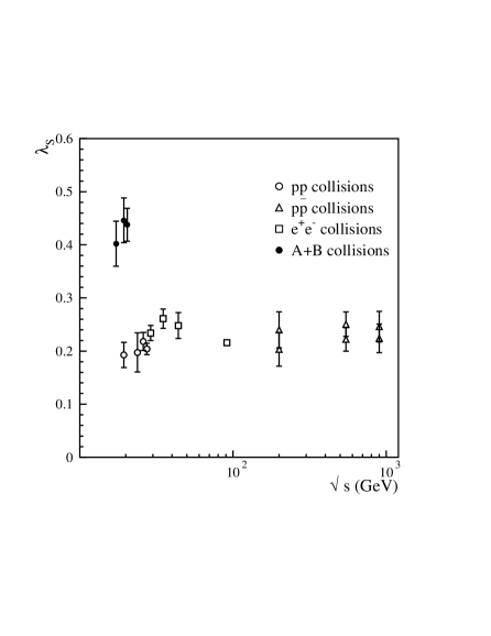
Fig. 4.11: By the measure in Eq. (4.2.2), global strangeness production is enhanced by a factor of $\sim 2$ in A-B [S-S, S-Ag, Pb-Pb] collisions cf. $e^{+}$-$e^{-}$, $p$-$p$, $p$-$\bar{p}$. The data are from Refs. [253]. (Adapted from Ref. [252]).

5 Toward a Kinetic Description

Hitherto we have described features of cold, sparse QCD: the nature of DCSB, confinement and bound state properties, and then the effect that the intensive thermodynamic parameters chemical potential and temperature have on these phenomena. In the latter we applied the methods of equilibrium statistical field theory and elucidated properties of the QGP phase. The terrestrial creation of this QGP, however, is expected to be effected via relativistic heavy ion collisions, which initially yield a quantum system far from equilibrium. This system must then evolve to form the plasma, and the study of that evolution and the signals that characterise the process are an important contemporary aspect of QGP research.

5.1 Preliminaries

The energy density in an ideal gas of eight gluons and two flavours of massless quarks is

$$\epsilon_{g+u+d}=(2\times 8)\,\frac{\pi^{2}T^{4}}{30}+(2\times 3\times 2)\,\frac{7\pi^{2}T^{4}}{120}=\frac{37\pi^{2}T^{4}}{30}\,.$$ (5.1.1)

As we saw in connection with Table 3.1, the critical temperature for QGP formation is $T_{c}\simeq 0.15\,$GeV and at this temperature: $\epsilon_{g+u+d}=0.8\,$GeV/fm³. Construction of RHIC at Brookhaven National Laboratory is complete and it will soon provide counter-circulating, colliding $100\,$A GeV $\,{}^{197}\!$Au beams to generate a total centre-of-mass energy of $40\,$TeV, which corresponds to an initial energy density: $\epsilon\sim 10$–$100\,$GeV/fm³. The Large Hadron Collider [LHC] project at CERN is scheduled for completion in 2005. Plans are for it to provide ²⁰⁸Pb-²⁰⁸Pb collisions with $\sqrt{s}\mathrel{\hbox to0.0pt{\lower 4.0pt\hbox{\hskip 0.0pt$\sim$}\hss}\raise 1.0pt\hbox{$>$}}2\,000\,$TeV and a consequent initial energy density $\epsilon\mathrel{\hbox to0.0pt{\lower 4.0pt\hbox{\hskip 0.0pt$\sim$}\hss}\raise 1.0pt\hbox{$>$}}1\,000\,$GeV/fm³. With these energy scales RHIC and LHC should certainly provide the conditions necessary for QGP formation.

Control over the conditions produced in a relativistic heavy ion collision can only be exerted via two experimental parameters: the beam/target properties and, to some extent, the impact parameter. They can be used together to analyse the debris collected in the detectors. It is in the behaviour of this debris, summed over many events, that signals of the evolution and formation of a QGP must be found. Predicting just what the signals are requires an understanding of these processes, including and perhaps especially their the non-equilibrium aspects.

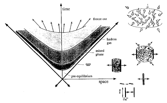
Fig. 5.1: Spacetime evolution of a relativistic heavy ion collision. Two [Lorentz contracted] disc-like nuclei collide and pass through each other, transforming a large amount of their kinetic energy into the potential energy of a highly excited spacetime volume. This energy is dissipated via particle production, which is a non-equilibrium process. The system evolves to equilibrium, expanding and passing through the QGP phase, hadronisation and freeze-out, where the observable hadronic debris is created. (Adapted from Ref. [255].)

Figure 5.1 illustrates the spacetime evolution of a relativistic heavy ion collision. All stages subsequent to the formation of a thermalised QGP are adequately addressed using hydrodynamical models [256]. However, in this approach the plasma’s initial conditions [energy density, temperature, etc.] and EOS must be specified. These initial conditions can only be reliably determined by following the complete evolution of the system produced in the collisions; i.e., by understanding the pre-equilibrium stage. Furthermore, the very existence of a pre-equilibrium phase can lead to signals of QGP formation; e.g., plasma oscillations, a disoriented chiral condensate [257], and out-of-equilibrium photon and dilepton emission [258].

The QGP is a hot, equilibrated, many-parton agglomeration, and in recent years two main approaches have been employed in describing how such a system might be produced in a relativistic heavy ion collision. In the perturbative parton picture [259], the colliding nuclei are visualised as pre-formed clouds of quarks and gluons. The collision proceeds via rapid, multiple, short-range parton-parton interactions, which generate entropy and transverse energy in a cascade-like process. In the string picture [260], after passing through one another, the colliding nuclei are imagined to stretch a high energy-density flux tube between them, which decays via a nonperturbative particle-antiparticle production process. Each approach has its merits and limitations, and their simultaneous pursuit provides complimentary results. The analysis of data proceeds via one of the many Monte-Carlo event generators that have been developed for both pictures [261, 262, 263].

Flux Tube Model and Schwinger Mechanism.    One intuitively appealing, semi-classical picture of confinement is provided by the notion that it is effected via the formation of a small-diameter colour flux tube between colour sources; and there is evidence in lattice simulations for the appearance of such flux tubes between heavy-quark-antiquark pairs; e.g., Ref. [264]. This is a motivation for the string-like models just introduced, which have been used to study particle production in $e^{-}$-$e^{+}$, $p$-$p$ and $p$-nucleus collisions [260, 265]. A flux tube yields a linearly-rising, confining quark-antiquark potential: $V_{q\bar{q}}(r)=\sigma\,r$, where the string tension: $\sigma$, can be estimated in static-quark lattice simulations. An overstretched flux tube can be viewed as a strong background field. As such it destabilises the QCD vacuum, which is corrected by particle-antiparticle production via a process akin to the Schwinger mechanism in QED [266, 267]. We use this particle production mechanism as the primary medium for our discourse.

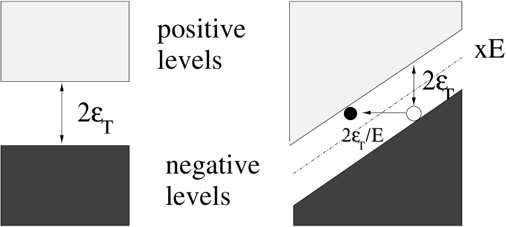
Fig. 5.2: Left Panel: For $E=0$ the vacuum is characterised by a completely filled negative-energy Dirac sea and an unoccupied positive-energy continuum, separated by a gap: $2\,\varepsilon_{\rm T}=2\,(m^{2}+p_{\perp}^{2})^{1/2}$. Right Panel: Introducing a constant external field: $\vec{E}=\hat{e}_{x}E$, which is produced by a potential: $A^{0}=-E\vec{x}$, tilts the energy levels. In this case a particle in the negative-energy sea will tunnel through the gap with a probability $\sim\exp(-\pi\varepsilon_{T}^{2}/eE)$. Succeeding, it will be accelerated by the field in the $-x$-direction, while the hole it leaves behind will be accelerated in the opposite direction. The energy-level distortion is increased with increasing $E$ and hence so is the tunnelling probability. [NB. $\tau_{\rm tu}\sim\varepsilon_{T}/eE$ is a measure of the time between tunnelling events. $eE$ can be related to the flux-tube string-tension.]

The fermion production rate for a constant, homogeneous electric field $E$ in a flux tube is [265]

$$S(p_{\perp})=\frac{dN}{dtdVd^{2}p_{\perp}}=|eE|\ln\bigg{[}1+\exp\bigg{(}-\frac{2\pi(m^{2}+p_{\perp}^{2})}{|eE|}\bigg{)}\bigg{]},$$ (5.1.2)

where $m$ is the mass and $e$ the charge of the produced particles, and it is plain from this formula that the rate increases with increasing $E$ and is suppressed for large $m$ and/or $p_{\perp}$. Particle-antiparticle production via this mechanism is analogous to a tunnelling process in quantum mechanics, as illustrated in Fig. 5.2. [NB. The Schwinger formula [266] follows immediately by integrating Eq. (5.1.2) over the transverse momentum: $\int d^{2}p_{\perp}$.]

What happens once the particles are produced? Naturally, they are accelerated in the tube by the field. This produces currents, which generate an electric field that works to screen the flux-tube [background] field. In the absence of other effects, the net field vanishes and particle production stops. However, the currents persist, now generating a field and renewed particle production that opposes their own existence. That continues until the net current vanishes. But at this point there is again a strong electric field … and the process repeats itself. This is the “back-reaction” phenomenon and the obvious consequence is time-dependent fields and currents; i.e., plasma oscillations characteristic of the system. In recent years its affects have been studied in both boson and fermion production [268] and we exemplify the process in Sec. 5.3.

There are a number of shortcomings in extant applications of the flux-tube particle-production picture to QGP formation: 1) The non-Abelian nature of the chromoelectric field is often ignored because the QCD analogue of the Schwinger mechanism is poorly understood. Instead the flux tube is represented via a classical electromagnetic potential; 2) On the whole, finite volume effects are neglected, with the electric field assumed to be homogeneous in space. A more realistic description would account for the geometry of the interaction region. Some steps have been taken in this direction, with a consideration of effects produced by a cylindrical boundary [269] and those in a finite-length flux tube with a confining transverse potential [270]. Going further, the geometrical representation of a flux tube can be replaced, allowing the flux tube profile itself to be a dynamical quantity, whose presence and stability is affected by the charged particle currents [271]; 3) The time-evolution of the system is described using either mean-field theory, which retains quantum effects but makes problematic an exploration of the effects of collisions, or a transport equation [272], which neglects quantum effects. Below we will describe a partial reconciliation of these approaches; and 4) Little attention has been paid to particular non-Abelian features in transport equations [273]. A study [274] of Wong’s equation [275] is one step in the direction of explicitly including colour algebra effects.

Quantum field theory can be applied directly to out-of-equilibrium plasma phenomena; for example, Refs. [268, 276]. However, kinetic equations provide an appealing alternative because of their intuitive character. This approach begins with a transport equation

$$p^{\mu}\,\frac{\partial f}{\partial q^{\mu}}-Q\,p^{\mu}F_{\mu\nu}\,\frac{\partial f}{\partial p_{\nu}}=S(p,q)+C(p,q)\,,$$ (5.1.3)

where: $f$ is the single particle distribution function, which gives the ensemble fraction of particles in a given phase-space cell [$p$ is four-momentum and $q$ is a spacetime four-vector]; $F_{\mu\nu}$ is the field strength tensor; and $Q$ is the particles’ charge. The source term: $S(p,q)$, describes the production of particle-antiparticle pairs and $C(p,q)$ is the collision term, whose origin is intuitively obvious but which is difficult to approximate accurately.

A Boltzmann equation of this form has been widely applied to particle production using a source term of the type in Eq. (5.1.2) both with and without a collision term, and in the following we exemplify this. However, to provide an introductory overview, Refs. [272] employ a classical, Abelian electric field in the source term but completely ignore the effect of collisions, $C\equiv 0$ in Eq. (5.1.3). The effect of collisions, represented via a “relaxation time approximation,” [described in connection with Eq. (5.4.2)] has been considered in an hydrodynamical approximation to Eq. (5.1.3), Refs [277, 278], with the influence of back-reactions neglected in the former but explored in the latter. A comparison between the transport equation and mean-field theory approaches has also been made [268] and the results are remarkably similar. That, however, is problematic since; e.g., the application of the Schwinger source term in the presence of a rapidly changing electric field is a priori unjustified and, although quantum field theory with its manifest microscopic time reversal invariance must underly the behaviour all quantum systems, experience confirms that systems far from equilibrium exhibit macroscopically irreversible behaviour that is amenable to treatment using [inherently time-irreversible] kinetic theory. The nature of the connection has recently been established [279, 280, 281].

At this point we re-emphasise that flux-tube models describe the nonperturbative production of soft partons. The production of hard and semi-hard partons is described by perturbative QCD and that mechanism is explored in Refs. [282]. Simultaneously incorporating both types of particle production is challenging but Ref. [283] is a step in that direction. Therein hard and semihard partons are produced via “minijet gluons” and provide the initial conditions necessary to solve the transport equations, and the subsequent evolution of the plasma is described by a classical but non-Abelian transport equation. Collisions are accounted for using a relaxation time approximation but quantum effects in the source term are neglected and, as will become apparent, they can be important in strong fields.

5.2 Quantum Vlasov Equation

The derivation of a quantum Vlasov equation in Refs. [279, 280, 281] provides a connection between the quantum field theoretical and transport equation approaches to particle production and plasma evolution, and shows that the particle source term is intrinsically non-local in time; i.e., non-Markovian. Therefore calculating the plasma’s properties at any given instant requires a complete knowledge of the history of the formation process.

The derivation begins with the Dirac [Klein-Gordon] equation for fermions [bosons] in an external, time-dependent, spatially homogeneous vector potential: $A_{\mu}$, in Coulomb gauge: $A_{0}=0$, taken to define the $z$-axis: ${\vec{A}}=(0,0,A(t))$. The corresponding electric field is

$$E(t)=-{\dot{A}}(t)=-\frac{dA(t)}{dt}\,,$$ (5.2.1)

also along the $z$-axis. The vacuum instability created by this external field is corrected via particle-antiparticle production, Fig. 5.2, which is a time-dependent process. The transition from the in-state to the instantaneous, quasi-particle state at time $t$ is achieved by a time-dependent Bogoliubov transformation, which effects the diagonalisation of the system’s Hamiltonian. By this means one obtains a kinetic equation for the single particle distribution function

$$f(\vec{P},t)=\langle 0|a^{\dagger}_{\vec{P}}(t)\,a_{\vec{P}}(t)|0\rangle\,,$$ (5.2.2)

which is defined as the vacuum expectation value, in the time-dependent basis, of creation and annihilation operators: $a^{\dagger}_{\vec{P}}(t)$, $a_{\vec{P}}(t)$, for particle states at time $t$ with three-momentum $\vec{P}$. That equation is

$$\frac{df_{\pm}({\vec{P}},t)}{dt}=\frac{\partial f_{\pm}({\vec{P}},t)}{\partial t}+eE(t)\frac{\partial f_{\pm}({\vec{P}},t)}{\partial P_{\parallel}(t)}=\frac{1}{2}{\cal W}_{\pm}(t)\int_{-\infty}^{t}dt^{\prime}{\cal W}_{\pm}(t^{\prime})[1\pm 2f_{\pm}({\vec{P}},t^{\prime})]\cos[x(t^{\prime},t)]\,,$$ (5.2.3)

where the lower [upper] sign in Eq. (5.2.3) corresponds to fermion [boson] pair creation. The momentum is defined as ${\vec{P}}=(p_{1},p_{2},P_{\parallel}(t))$, with the longitudinal [kinetic] momentum $P_{\parallel}(t)=p_{\parallel}-eA(t)$, $p_{\parallel}=p_{3}$. [NB. $eE(t)={\dot{P}_{\parallel}}(t)$, the particle velocity attained via acceleration by the field $E(t)$.] For fermions [279, 280] and bosons [280, 281] the transition amplitudes are

$${\cal W}_{-}(t)=\frac{eE(t)\varepsilon_{\perp}}{\omega^{2}(t)}\,,\;\;{\cal W}_{+}(t)=\frac{eE(t)P_{\parallel}(t)}{\omega^{2}(t)}\,,$$ (5.2.4)

where the transverse energy $\varepsilon_{\perp}=\sqrt{m^{2}+\vec{p}_{\perp}^{\,2}}$, ${\vec{p}}_{\perp}=(p_{1},p_{2})$, and $\omega(t)=\sqrt{\varepsilon_{\perp}^{2}+P_{\parallel}^{2}(t)}$ is the total energy. In Eq. (5.2.3),

$$x(t^{\prime},t)=2[\Theta(t)-\Theta(t^{\prime})]\,,\;\;\Theta(t)=\int^{t}_{-\infty}dt^{\prime}\omega(t^{\prime})\,,$$ (5.2.5)

is the dynamical phase difference. Equation (5.2.3) is the precise analogue of directly solving QED with an external field in mean-field approximation, as done; e.g., in Ref. [268]. The physical content is therefore equivalent and, in particular, the fundamental quantum character is preserved. The appeal of this kinetic equation, however, is that it simplifies: the identification of reliable approximations; widespread applications; and numerical studies.

This quantum Vlasov equation has three qualitatively important features: 1) The source is non-Markovian for two reasons – (i) the source term on the r.h.s. requires complete knowledge of the distribution function’s evolution from $t_{-\infty}\rightarrow t$; and (ii) the integrand is a non-local function of time, which is apparent in the coherent phase oscillation term $\cos x(t^{\prime},t)$ and reflects the quantum nature of the source term; 2) Particles are produced with a momentum distribution cf. the Schwinger source term, which produces particles with zero longitudinal momentum; and 3) the production rate is affected by the particles’ statistics, as evident in Eqs. (5.2.4) and also in the sign appearing in the statistical factor $[1\pm 2f_{\pm}]$, which leads to different phase space occupation [284].

These features can have a material impact on the solution of the kinetic equation, and their importance depends on the field strength and the time-scales characterising the production process. The first time-scale is set by the Compton wavelength of the produced particles:

$$\tau_{\rm qu}\sim\frac{1}{\varepsilon_{\perp}}\,.$$ (5.2.6)

Events taking place over times less-than this expose the negative-energy elements in particle wave-packets, a core quantum field theoretical feature. This is the time-scale of the rapid oscillations generated by the dynamical phase difference in $\cos x(t^{\prime},t)$. The high frequencies involved mean that the main contributions arise when $t\sim t^{\prime}$, and therefore a local approximation can be justified for weak field plasmas [281]. We identified a second time-scale in Fig. 5.2; i.e., the time taken for a particle to tunnel through the barrier. It can also be motivated by considering the transition amplitudes in Eqs. (5.2.4), which for a constant electric field can be written in the form; e.g.,

$${\cal W}_{-}(t)=\frac{\varepsilon_{\perp}/eE}{(t-p_{\parallel}/eE)^{2}+(\varepsilon_{\perp}/eE)^{2}}\,,$$ (5.2.7)

which is a Lorentzian characterised by the time-scale [width]

$$\tau_{\rm tu}\sim\frac{\varepsilon_{\perp}}{eE}\,.$$ (5.2.8)

This is also the time required to accelerate a charged particle to the speed of light in an electric field.

The times scales in Eqs. (5.2.6) and (5.2.8) are comparable when $eE\sim\varepsilon_{\perp}^{2}$. For weak fields, $\tau_{\rm qu}\ll\tau_{\rm tu}$ and, in the integrand on the r.h.s. of Eq. (5.2.3), the $\cos x(t^{\prime},t)$ oscillations occur on a time-scale so-much shorter than variations in the other elements that a stationary phase approximation is valid. That approximation yields a local source term and this important limit of Eq. (5.2.3) was discussed in Ref. [281].

$\tau_{\rm tu}\mathrel{\hbox to0.0pt{\lower 4.0pt\hbox{\hskip 0.0pt$\sim$}\hss}\raise 1.0pt\hbox{$>$}}\tau_{\rm qu}$ for strong fields and hence the particle’s Compton wavelength extends across the gap. In this case wave-like [quantum] interference effects become important in the behaviour of $f(p,q)$, which changes at a rate comparable with $\cos x(t^{\prime},t)$, so that a stationary phase approximation is not valid. Can this strong field scenario be relevant to contemporary relativistic heavy ion collisions? It is easy to make an estimate. The field strength in a flux tube is commensurate with the QCD string tension; i.e., $eE\sim\sigma\approx 0.4\,$GeV${}^{2}\sim(2.5\,\Lambda_{\rm QCD})^{2}$, and $\varepsilon_{\perp}\sim 2$–$3\,\Lambda_{\rm QCD}$ is achievable. Therefore the answer is yes: effects arising from the non-Markovian structure of the source term are likely to be exhibited in contemporary relativistic heavy ion collisions.

This was illustrated in Ref. [285], wherein a comparison was made between the complete solution and that obtained in the low density limit; i.e., retaining $\cos x(t^{\prime},t)$ in the source term but making the replacement $[1\pm 2f_{\pm}]\to 1$, which is the assumption

$$f_{\pm}\simeq 0\,,\;{\rm almost~{}everywhere,}$$ (5.2.9)

so that the source term becomes

$$S^{0}_{\pm}({\vec{p}},t)=\mbox{\footnotesize$\frac{1}{2}$}{\cal W}_{\pm}(t)\int_{-\infty}^{t}dt^{\prime}{\cal W}_{\pm}(t^{\prime})\cos x(t^{\prime},t)\,.$$ (5.2.10)

Using Eq. (5.2.10), the solution of Eq. (5.2.3) is

$$f^{0}_{\pm}({\vec{p}},t)=\int_{-\infty}^{\,t}\,dt^{\prime}S_{\pm}^{0}({\vec{p}},t^{\prime})\,,$$ (5.2.11)

and is depicted for fermions in Fig. 5.3.

Fig. 5.3: Time-evolution in a constant electric field of the complete single fermion distribution function cf. that obtained in the low-density limit, Eq. (5.2.9), with $p_{\|}=0=p_{\perp}$ and initial condition $f(t\rightarrow-\infty)=0$. Upper Panel: Strong field, $eE_{0}/m^{2}=3.0$; Lower Panel: Weak field, $eE_{0}/m^{2}=0.5$. (Energy unit: $m\approx\Lambda_{\rm QCD}$. Adapted from Ref. [285].)

Particle production begins at $t=0$ because, with $p_{\|}=0$, the transition amplitudes in Eq. (5.2.4) are maximal at this point [the vector potential is zero], and the distribution function rapidly approaches a Schwinger-like asymptotic value:

$$f^{\rm full}(t\rightarrow\infty)=\exp(-\pi\varepsilon_{\perp}^{2}/eE)=\begin{array}[]{ccc}e^{-\pi/3}&\approx&0.35\;({\rm strong})\\ e^{-2\pi}&\approx&0.0019\;({\rm weak})\end{array}\,.$$ (5.2.12)

The qualitative features of the results depicted in Fig. 5.3 are easily understood. A fermion, once produced with a certain momentum, retains it because there are no further interactions [collisions are ignored]. The number density is greater for strong fields because they produce more particles and this plainly means that the low-density limit will smoothly become invalid with increasing field strength. The low-density limit overestimates the fermion distribution function in strong fields because it eliminates Pauli blocking. The opposite effect is seen for bosons [285]. For very strong fields: $f_{-}\to 1$, again because of Pauli blocking, but there is no such bound on the boson distribution function. Finally, since $\sigma/\varepsilon_{\perp}^{2}>3$ is achievable in contemporary relativistic heavy ion collisions, the low-density limit is quantitatively unreliable.

5.3 Back-reactions

The illustration above assumed a constant electric field. Allowing the more realistic case of a time-dependent field introduces another time-scale, namely that characterising the response of the field to the system’s evolution. This brings us to the phenomenon of back-reactions, which have been explored in connection with models in cosmology and recently much in connection with QGP evolution. In both cases the particles produced by the strong background field modify that field: in cosmology it is the time-dependent gravitational field, which couples via the masses, and in a QGP, it is the chromoelectric field affected by the partons’ colour charge.

The effect of feedback is incorporated by solving Maxwell’s equation, which for a spatially homogeneous but time dependent electric field is just

$$\dot{E}(t)=-j(t)\,.$$ (5.3.1)

The total field is a sum of two terms: an external field, $E_{ex}(t)$, excited by an external current, $j_{ex}(t)$, such as might represent a heavy ion collision [that is a model input]; and an internal field, $E_{in}(t)$, generated by the internal current, $j_{in}(t)$, which characterises the behaviour of the particles produced. The internal current has two components [277]: continued spontaneous production of charged particle pairs creates a polarisation current, $j_{pol}(t)$, that depends on the particle production rate, $S({\vec{p}},t)$; and the motion of the existing particles in the plasma generates a conduction current, $j_{cond}(t)$, that depends on their momentum distribution, $f({\vec{p}},t)$. The internal field is therefore obtained from

$$-{\dot{E}}_{in}(t)=j_{in}(t)=j_{cond}(t)+j_{pol}(t)\,.$$ (5.3.2)

In mean field approximation the currents can be obtained directly from the constraint of local energy-density conservation: $\dot{\epsilon}=0$, where

$$\epsilon(t)=\mbox{\footnotesize$\frac{1}{2}$}E^{2}(t)+2\int\!\mbox{\footnotesize$\frac{d^{3}p}{(2\pi)^{3}}$}\,\omega(\vec{p},t)\,f(\vec{p},t)\,,$$ (5.3.3)

and the factor of $2$ accounts for antiparticles. For bosons the constraint yields

$${\dot{E}}(t)=-2e\int\!\mbox{\footnotesize$\frac{d^{3}p}{(2\pi)^{3}}$}\,\frac{p_{\parallel}-eA(t)}{\omega({\vec{p}},t)}\bigg{[}f({\vec{p}},t)+\frac{\omega({\vec{p}},t)}{{\dot{\omega}}({\vec{p}},t)}\frac{df({\vec{p}},t)}{dt}\bigg{]}\,,$$ (5.3.4)

and one easily identifies the currents

$$j_{cond}(t)=2e\int\!\mbox{\footnotesize$\frac{d^{3}p}{(2\pi)^{3}}$}\,\frac{p_{\parallel}-eA(t)}{\omega({\vec{p}},t)}f({\vec{p}},t)\,,\;\;j_{pol}(t)=\frac{2}{E(t)}\int\!\mbox{\footnotesize$\frac{d^{3}p}{(2\pi)^{3}}$}\,\omega({\vec{p}},t)S({\vec{p}},t)\,.$$ (5.3.5)

Equation (5.3.2) now yields the internal field. This construction has been used extensively to study back-reactions; e.g., Refs. [268, 286].

The expression for the polarisation current exhibits the usual short-range divergence associated with charge renormalisation, however, its regularisation and renormalisation is straightforward [268, 286]. That accomplished, Maxwell’s equation assumes the form

$$-{\ddot{A}}^{\pm}(t)={\dot{E}}^{\pm}(t)=-j^{ex}(t)$$

$$-g_{\pm}e\int\!\mbox{\footnotesize$\frac{d^{3}P}{(2\pi)^{3}}$}\,\frac{P_{\parallel}(t)}{\omega({\vec{P}},t)}\left[f_{\pm}({\vec{P}},t)+\frac{1}{2}\left\{2\frac{S({\vec{P}},t)}{{\cal W}_{\pm}({\vec{P}},t)}-\frac{e\,\dot{E}^{\pm}(t)\,P_{\parallel}(t)}{4\,\omega^{4}(\vec{P},t)}\right\}\bigg{(}\frac{\epsilon_{\perp}}{P_{\parallel}(t)}\bigg{)}^{g_{\pm}-1}\right]\,,$$

where $g_{-}=2$, $g_{+}=1$, and all fields and charges are understood to be fully renormalised.

Fig. 5.4: Time evolution for bosons of the electric field and current for an impulse external field, Eq. (5.3.7), with $A_{0}=10.0$, $b=0.5$ and the coupling $e^{2}=5$. The plasma oscillations driven by the back-reactions are evident. A complete explanation of the qualitative features evident here is given after Eq. (5.3.7). (Energy unit: $m\approx\Lambda_{\rm QCD}$. Adapted from Ref. [286]).

The effect of back-reactions can now be illustrated by solving this equation in concert with Eq. (5.2.3). [Collisions are still neglected: $C\equiv 0$ in Eq. (5.1.3).] A relativistic heavy ion collision can be mimicked by an impulse profile for the external field [286]:

$$E_{ex}(t)=\,-\,\frac{A_{0}}{b}\,{\rm sech}^{2}(t/b)\,,$$ (5.3.7)

which “switches-on” at $t\sim-2b$ and off at $t\sim 2b$, with a maximum magnitude of $E_{\rm max}=A_{0}/b$ at $t=0$. Once this field has vanished only the induced internal field remains to create particles and affect their motion. The calculated field and current profiles are depicted in Fig. 5.4, and the qualitative features are easily understood. The impulse electric field is evident at $t\simeq 0$. It produces particles and accelerates them, and their motion generates an internal current that opposes the impulse field. Shortly after the “collision” the current reaches a short-lived plateau, when the total field vanishes and particle production halts temporarily. At about this time the external, collision-mimicking field “turns-off.” Nevertheless, in its absence, the total field grows in magnitude but now acts in the opposite direction, decelerating the existing particles, causing new particles to be produced and accelerating them in the new direction. The effect of that is clear, after a time the total current must vanish. A pattern is now established and, in the absence of other influences such as collisions or radiation, it repeats itself, reaching a steady state once the wash from the collision-mimicking impulse configuration disappears completely. The oscillations characteristic of a plasma with field-current feedback have now set-in. The oscillation period is the new time scale:

$$\tau_{\rm pl},\,{\rm the~{}plasma~{}period.}$$ (5.3.8)

It decreases with increasing field strength.

Fig. 5.5: $f(p,t={\rm fixed})$. The rapid oscillations are a quantum coherence effect, a manifestation of interference between effects on the $\tau_{\rm qu}$ and $\tau_{\rm tu}$ time-scales. Employing a local [or stationary phase or Markov] approximation to the source term, these effects are averaged-out. (Energy unit: $m\approx\Lambda_{\rm QCD}$. Adapted from Ref.[281].)

One more feature of the results is the high frequency oscillations evident at the current’s peaks and troughs. They are not a numerical artefact and become more pronounced with increasing values of $eE/m^{2}$; i.e., when $\tau_{\rm qu}\simeq\tau_{\rm tu}$. This makes plain that they are a non-Markovian feature and result from interference between effects on the tunnelling and quantum time-scales. Of course, as illustrated via an analogous feature in Fig. 5.5, they disappear if a local approximation to the source term is used [281] because the stationary phase approximation suppresses such interference effects.

One additional observation is important here. Our example employed an electric field whose magnitude, $\propto A_{0}$, is large and hence the tunneling time, $\tau_{tu}$, is small, being inversely proportional to $eE$. The period of the plasma oscillations, $\tau_{pl}$, also decreases with increasing $A_{0}$ but nevertheless, as clear in Fig. 5.4, $\tau_{tu}\ll\tau_{pl}$. Thus, in contrast to the effect it has on the production process [285], the temporal nonlocality of the non-Markovian source term is unimportant to the collective plasma oscillation [286]. This is the reason why kinetic equations with a simple source term of the form in Eq. (5.1.2) are successful in describing plasma oscillations [268]. Whether or not these oscillations are observable in relativistic heavy ion collisions depends on the effect of dissipative processes, which we now discuss.

5.4 Collisions and Evolution of the Quark-Gluon Plasma

Thus far we have illustrated the phenomena of quantum particle production in strong fields and field-current feedback. The stationary state is unrealistic because the dissipative processes: “collisions,” that lead to thermalisation have been neglected. [Collisions can also lead to particle production and effect hadronisation but we defer that discussion.]

In the presence of collisions the kinetic equation takes the form

$$\frac{df_{\pm}({\vec{p}},t)}{dt}=S_{\pm}({\vec{p}},t)+C_{\pm}({\vec{p}},t)\,.$$ (5.4.1)

A simple and widely-used model [278, 287, 288, 289, 290] for the collision term is

$$C_{\pm}({\vec{p}},t)=\frac{f_{\pm}^{eq}({\vec{p}},t)-f_{\pm}({\vec{p}},t)}{\tau_{\rm r}}\,,$$ (5.4.2)

where $\tau_{\rm r}$ is the “relaxation time” and $f^{eq}$ is the thermal equilibrium distribution function

$$f_{\pm}^{eq}({\vec{p}},t)=\frac{1}{\exp[\omega({\vec{p}},t)/T(t)]\mp 1}\,,$$ (5.4.3)

with $T(t)$ a time-dependent temperature profile, discussed on page 5.6. The relaxation time is a fourth time-scale and it is plain that plasma oscillations can only be observable if $\tau_{\rm pl}\ll\tau_{\rm r}$; i.e., if collisions take place much-less frequently than oscillations.

In many of the exploratory calculations hitherto undertaken, $\tau_{\rm r}$ is a constant. That might be argued to be inadequate because the collision time is supposed to characterise a system’s thermalisation, a process which is interdependent with time-evolving quantities such as density and temperature. A more realistic representation might therefore employ a time-dependent $\tau_{\rm r}$, which is calculated self-consistently as the plasma evolves. Reference [291], employing collisions in a gluon-minijet plasma, is a step in that direction. However, from another perspective, any sophisticated collision term should be derived from, and justified by, an underlying microscopic theory (see; e.g., Refs. [273, 279, 292].); and, furthermore, a relaxation time approximation of any sort can only be valid under conditions of quasi-equilibrium, which cannot be justified a priori in the presence of strong fields. A truly realistic collision term will introduce non-Markovian effects in addition to those already present in the source term, and exemplary studies exist in connection with: relativistic heavy ion collisions [293]; collective effects in nuclear matter [294]; nuclear fragmentation [295]; and the damping rates of giant dipole resonances [296]. These studies make clear that even a binary collision approximation, as characteristic of a Boltzmann-Uehling-Uhlenbeck kinetic equation, can be inadequate under extreme conditions; e.g., in the presence of strong fields and/or when the particle density is high. These are precisely the conditions relevant to QGP formation. The patent complexity justifies the use in exploratory, illustrative studies of the simple $\tau_{\rm r}=\,$constant relaxation time approximation. Improvements are a contemporary challenge.

Fig. 5.6: Time evolution for bosons of the electric field obtained using different relaxation times in the collision term of Eq. (5.4.2), and with the impulse external field, Eq. (5.3.7), where $A_{0}=7.0$, $b=0.5$ and the coupling $e^{2}=4$. (Energy unit: $m\approx\Lambda_{\rm QCD}$. Adapted from Ref. [286].)

As intuition suggests, collisions effect a damping of the distribution functions’ time-dependent structure. That is illustrated in Fig. 5.6, with this particular calculation obtained using an Ansatz for the temperature profile [286]

$$T(t)=T_{eq}+(T_{m}-T_{eq})\,{\rm e}^{-t^{2}/t_{0}^{2}}\,,$$ (5.4.4)

where $T_{eq}=\Lambda_{\rm QCD}$, $T_{m}=2\,T_{eq}$, $t_{0}^{2}=10/\Lambda_{\rm QCD}$. [The definition and meaning of $T(t)$ is discussed below.] As evident in the figure, for large relaxation times the plasma oscillations are unaffected, as might be anticipated because this is the collisionless limit. However, for $\tau_{\rm r}\sim\tau_{\rm pl}$, the collision term has a significant effect, with both the amplitude and frequency of the plasma oscillations being damped. Finally, there is a value of $\tau_{\rm r}$ below which oscillations are not possible, just as in the case of an overdamped harmonic oscillator, and the system evolves quickly and directly to thermal equilibrium. The time taken by the plasma to thermalise depends on the ratio $\tau_{\rm pl}/\tau_{\rm r}$, being longer for larger values.

Why use the temperature profile in Eq. (5.4.4) and, indeed, what is temperature in a system far from equilibrium? The notion of temperature is introduced via an assumption of quasi-equilibrium at each time $t$, which is only truly valid if the fields are not too strong; i.e., only as long as $\tau_{\rm tu}\gg\tau_{\rm pl}$. This temporally local temperature can be calculated self-consistently with the evolution of the distribution functions, an approach which represents a slight improvement over employing Ansätze, such as Eq. (5.4.4), and, in fact, can provide an a posteriori justification for that expedient. The calculation of $T(t)$ can, however, proceed in a number of ways so that the resulting profile is not unique but the differences are only small and quantitative.

To illustrate the definition of a temperature profile we follow Ref. [290]. The total energy density in the evolving plasma is given in Eq. (5.3.3), where the second term is the particle contribution: $\epsilon_{f}(t)$, and the particle number density is

$$n(t)=2\int\!\mbox{\footnotesize$\frac{d^{3}p}{(2\pi)^{3}}$}\,f_{-}({\vec{p}},t)\,.$$ (5.4.5)

An intuitive definition of the local temperature is to require that, at each $t$, the average energy-per-particle in the evolving plasma is that of a a quasi-equilibrium gas; i.e.,

$$\frac{\epsilon_{f}(t)}{n(t)}=\frac{\epsilon^{eq}(t)}{n^{eq}(t)}\,,$$ (5.4.6)

where

$$\epsilon^{eq}(t)=2\,\int\!\mbox{\footnotesize$\frac{d^{3}p}{(2\pi)^{3}}$}\,\omega({\vec{p}},t)f_{-}^{eq}({\vec{p}},t)\,,\;\;n^{eq}(t)=2\,\int\!\mbox{\footnotesize$\frac{d^{3}p}{(2\pi)^{3}}$}\,f_{-}^{eq}({\vec{p}},t)\,.$$ (5.4.7)

With $f_{-}^{eq}$ given in Eq. (5.4.3), Eq. (5.4.6) is an implicit equation for $T(t)$, which must be solved simultaneously with Eqs. (5.3) and (5.4.1) [290].

Fig. 5.7: Time evolution of the fermion’s energy density for RHIC (upper panel) and LHC (lower panel) conditions. For RHIC conditions, the result obtained using the low density approximation, Eq. (5.2.10), is indistinguishable from the complete solution. That is not the case for LHC-like conditions. (Adapted from Ref. [290].)

In Ref. [290], this system of equations was solved with $m=\Lambda_{\rm QCD}$, $e=2$, and $\tau_{\rm r}=1/\Lambda_{\rm QCD}\approx 1\,$fm, and using two exemplary impulse field configurations: Eq. (5.3.7), with $b=0.5/\Lambda_{\rm QCD}\approx 0.5\,$fm and either $A_{0}^{RHIC}=4\,\Lambda_{\rm QCD}$ or $A_{0}^{LHC}=20\,\Lambda_{\rm QCD}$. As evident in Fig. 5.7, $A_{0}^{RHIC}$ yields a calculated initial energy-density characteristic of RHIC conditions [see Sec. 5.1] while $A_{0}^{LHC}$ gives a very much greater value characteristic of the initial energy-density expected at LHC. For RHIC conditions the energy-density rises rapidly but, after reaching a maximum, decays monotonically. The low density approximation is valid here. For LHC conditions, with an initial energy-density twenty-times larger, the situation is different: the solution obtained in the low density limit is only a qualitative guide to the plasma’s evolution and plasma oscillations are evident on observable time-scales. These oscillations retard the equilibration of the plasma, roughly doubling the time taken cf. RHIC-like conditions. This application makes evident an expected terrestrial hierarchy of time-scales:

$$\tau_{\rm qu}\sim\tau_{\rm tu}<\tau_{\rm pl}\sim\tau_{\rm r}\,.$$ (5.4.8)

In a very intense field the produced particles travel almost at the speed of light and hence the plasma oscillation period can be estimated via the ultrarelativistic formula [297]:

$$\mbox{\footnotesize$\frac{1}{2}$}\tau^{UR}_{\rm pl}\approx\frac{\sqrt{n_{\rm max}\,m+E_{\rm max}^{2}}}{n_{\rm max}\,e}\approx 2\,,$$ (5.4.9)

using the input and LHC-like results of Ref. [290], which yield $n_{\rm max}\simeq 12/\Lambda_{\rm QCD}^{3}$ from Eq. (5.4.5). That this is a reliable guide for LHC-like conditions is evident in Fig. 5.7, remembering that $\epsilon(t)\sim E^{2}(t)$ so that the peaks exhibited in the lower panel are separated by $\mbox{\footnotesize$\frac{1}{2}$}\tau_{\rm pl}$.

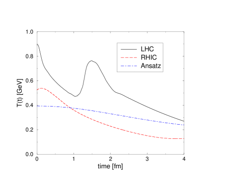
Fig. 5.8: Time evolution of the temporally local quasi-equilibrium temperature for RHIC and LHC initial conditions. For comparison we also plot the Ansatz in Eq. (5.4.4), which is a fair guide for RHIC-like conditions. (Adapted from Ref. [290].)

The calculated temperature profile is depicted in Fig. 5.8. Under RHIC-like conditions, an initial temperature of $T(t=0)\sim 0.5\,$GeV is reached and the temperature decreases monotonically. The LHC-like source conditions yield an initial temperature twice as large: $T^{\rm LHC}(t=0)\sim 0.9\,$GeV, and the temperature fluctuates in tune with the energy density.

As described above, the exemplary impulse models in Ref. [290] set initial energy density scales appropriate for RHIC and LHC. An improvement over such Ansätze is to calculate the initial conditions, as done; e.g., in Refs. [283, 291] for the case of a gluon minijet plasma. Even with this improvement, however, the results obtained for observable quantities; such as, $\epsilon(t)$, $n(t)$, the temperature and equilibration time, are semi-quantitatively identical and all features are qualitatively unchanged.

It is a uniform prediction that plasma oscillations are present under LHC-like conditions and they may manifest themselves in the dilepton spectrum. The dilepton production rate is (see; e.g., Ref. [298])

$$\frac{d\,N_{l^{+}l^{-}}}{dt\,d^{3}x}\sim\int d^{3}p_{1}d^{3}p_{2}\,f(E_{1})\,f(E_{2})\,\sigma(M)\,v_{12}\,,$$ (5.4.10)

where $f$ is the distribution function of the charged elements in the plasma, $\sigma(M)$ is the cross-section for particle-antiparticle annihilation into a dilepton pair with invariant mass $M$ and $v_{12}$ is the standard phase-space factor [a “relative particle-antiparticle velocity”]. The distribution function responsible for the features in Fig. 5.7 itself exhibits structure and, according to Eq. (5.4.10), that will be transmitted to the dilepton spectrum. The oscillations characterising the pre-equilibrium phase of the plasma could then be exhibited as repeated dilepton bursts. However, this signal will only be detectable if it is strong enough relative to other process, such as Drell-Yan. That quantitative question is currently unanswered.

5.5 Hadronisation

The penultimate stage of QGP evolution is hadronisation; i.e., the re-establishment of the conditions that prevail at zero density and temperature. That process in not instantaneous and hence here too a dynamical approach is necessary, one that provides the means of describing phenomena such as bound state formation, and the onset of DCSB and confinement. Consequently the development of a transport theory in which such effects are directly accessible is an important current focus.

Relativistic transport theory and hydrodynamics have long been useful tools in the study of non-equilibrium states of matter at nonzero density and temperature. They have been employed extensively in relativistic nuclear physics, both in the intermediate energy region [292, 299], where it may be appropriate to neglect quark and gluon degrees of freedom, and in the high energy domain directly relevant to a non-equilibrium QGP [262, 300, 301, 302]. One approach [303] to the derivation of Vlasov-like transport equations can be described as a relativistic generalisation of the Zubarev method [304]. Another is the contour Green function technique [305], which has been applied formally; e.g., in Refs. [300, 301, 302], and also in quantitative model studies; e.g., Refs. [306, 307, 308, 309, 310]. The latter is widely used because it admits a systematic definition and exploration of approximations, and will be our focus.

To be concrete, extant phenomenological applications begin with a model Lagrangian density; e.g., that of the Friedberg-Lee or Nambu–Jona-Lasinio model. Such models are chosen because of their efficacy in describing DCSB, and have been employed in studies of: the spacetime evolution of the dressed-quark mass [306, 307, 308, 309], which characterises the onset of DCSB; and hadronisation via the models’ fermion-antifermion–bound-state interaction terms [310]. In the former case, the onset of DCSB is explored by solving a quantum Vlasov equation coupled with a distribution-function-dependent gap equation, which describes the evolution of the particles’ mass and feeds this information back into the system. One important qualitative result is a parton mass that increases as the system moves toward equilibrium; e.g., Ref. [307], which results in a dynamical softening of the EOS. This softening can have observable consequences; e.g., slowing the [hydrodynamical] expansion of the plasma [311]. These models, however, do not incorporate confinement and hence cannot describe the replacement of coloured degrees of freedom by hadronic matter through the transition.

An indication that the onset of confinement might significantly affect the evolution of the plasma was observed in Ref. [309], wherein a $T$-dependent dressed-quark mass was introduced by fitting the model’s quasi-particle energy density to that determined in lattice simulations. A self-consistent solution of the coupled Vlasov and gap equations then exhibits confinement; i.e., the partons cannot leave the QGP volume because their mass becomes infinite outside this region. The model does not include a parton-antiparton–hadron interaction and hence the confining effect also stops the hydrodynamical expansion. This study only admitted the importance of the scalar piece of the dressed-quark self energy. However, as we saw; e.g., in connection with Fig. 3.5, the vector self energy is more important in QCD’s deconfined domain. The effect it has on plasma evolution has not hitherto been explored.

The incorporation of such qualitatively robust features of DSE studies into the Vlasov equation is an obvious next step [237]. It is complicated for [at least] two reasons: 1) The quasi-particle energy is a functional of the scalar and vector dressed-quark self energies, which are both nonzero and momentum dependent. The scalar self energy is small in the QGP. [It vanishes in the chiral limit.] However, the significant vector self energy remains [176]; 2) In the confined domain the dressed-parton $2$-point functions violate reflection positivity and hence a single particle distribution function for these excitations cannot be defined. That is as it should be because hadrons are the relevant degrees of freedom in this phase: a kinetic theory based on quarks and gluons is only appropriate in the deconfined QGP phase. As described in connection with Fig. 3.3, DSE models can adequately represent the transition from confined excitation to propagating quasiparticle [181], an attribute exploited in Ref. [176] in calculating the thermodynamic functions describing a QGP. These observations suggest that a truly realistic description of the quark and gluon distribution functions in a QGP will see them vanish in the vicinity of the phase boundary.

We close this section with an illustration of the concepts introduced. In a QGP the evolution of the dressed-quark distribution function can be described using a Vlasov equation with the quasi-particle energy

$$E_{\ast}(\vec{p},\vec{x},t)=p_{0}\,[1+\Sigma_{C}(\vec{p},\vec{x},t)]=\sqrt{|\vec{p}_{\ast}|^{2}+B(\vec{p},\vec{x},t)^{2}}\,,$$ (5.5.1)

where ${\vec{p}}_{\ast}={\vec{p}}\,[1+\Sigma_{A}(\vec{p},\vec{x},t)]$ is the rescaled three-momentum and $B(\vec{p},\vec{x},t)=[m+\Sigma_{B}(\vec{p},\vec{x},t)]$. Using Eqs. (3.1.17), Eq. (5.5.1) can be rewritten

$$E_{\ast}(\vec{p},\vec{x},t)=C(\vec{p},\vec{x},t)\,E(\vec{p},\vec{x},t)=C(\vec{p},\vec{x},t)\,\sqrt{|\vec{p}|^{2}\,{\cal I}(\vec{p},\vec{x},t)^{2}+{\cal M}(\vec{p},\vec{x},t)^{2}}\,,$$ (5.5.2)

where ${\cal I}=A/C$ and ${\cal M}=B/C$. As our exemplar we follow Ref. [237] and employ an instantaneous variant of the ${\cal D}_{\rm A}$ model in Sec. 3.2:

$${\cal D}(p_{\Omega_{k}})=3\pi^{2}\,\eta\,\delta^{3}(\vec{p})\,.$$ (5.5.3)

With this interaction and using rainbow truncation, which is akin to a mean-field approximation, the Matsubara sum can be evaluated algebraically because the self energies are $p_{0}$-independent, and the gap equation assumes the form

$$B(\vec{p},\vec{x},t)=m+\eta\,\frac{B(\vec{p},\vec{x},t)}{E_{\ast}(\vec{p},\vec{x},t)}{f_{\ast}}(\vec{p},\vec{x},t)\,,\;\;C(\vec{p},\vec{x},t)=1+\mbox{\footnotesize$\frac{1}{2}$}\eta\,\frac{C(\vec{p},\vec{x},t)}{E_{\ast}(\vec{p},\vec{x},t)}{f_{\ast}}(\vec{p},\vec{x},t)\,,$$ (5.5.4)

with $A=C$, so that ${\cal I}=1$, and $f_{\ast}=f/C$. [NB. $f$ appears explicitly here because, with a quasiparticle pole, the Matsurbara sum can be evaluated algebraically.] Again, in spite of the model’s simplicity, the solution exhibits qualitative features that are characteristic of a realistic dressed-quark $2$-point function; e.g., momentum-dependent scalar and vector self energies, and the persistence of this aspect of the solutions in the deconfined domain [237]. In this class of models, for a collisionless plasma, $f_{\ast}$, satisfies [301]

$$0=\partial_{t}{f_{\ast}}(\vec{p},\vec{x},t)$$

$$+\frac{1}{E(\vec{p},\vec{x},t)}\,\left\{\left[{\vec{p}}+{\cal M}(\vec{p},\vec{x},t)\vec{\nabla}_{p}\,{\cal M}(\vec{p},\vec{x},t)\right]\cdot\vec{\nabla}_{x}{f_{\ast}}(\vec{p},\vec{x},t)-{\cal M}(\vec{p},\vec{x},t)\vec{\nabla}_{x}{\cal M}(\vec{p},\vec{x},t)\cdot\vec{\nabla}_{p}{f_{\ast}}(\vec{p},\vec{x},t)\right\}\,.$$

It is important to note that the dressed-quark mass function is momentum-dependent so that in general

$$\vec{\nabla}_{p}\,{\cal M}(\vec{p},\vec{x},t)\cdot\vec{\nabla}_{x}\,{f_{\ast}}(\vec{p},\vec{x},t)\neq 0\,.$$ (5.5.6)

[NB. The Vlasov equation in Ref. [309] is obtained by neglecting this term, since $\vec{\nabla}_{p}M\equiv 0$ when the interaction is momentum-independent, and setting $C=1$.] Equations (5.5.4) and (5.5) provide a coupled system for the quark’s distribution function and self energies.

As remarked above, the derivation of a transport equation like Eq. (5.5) requires the existence of a quasi-particle mass shell. The instantaneous model ensures that, with $p^{0}=E(\vec{p},\vec{x},t)$. In this case $\frac{\partial f_{\ast}}{\partial p^{0}}=0$ and $\frac{\partial{\cal M}}{\partial p^{0}}=0$, hence Eq. (5.5) can be written

$$p^{\mu}\,\partial^{x}_{\mu}f_{\ast}+{\cal M}\left\{\partial^{x}_{\mu}{\cal M}\,\partial_{p}^{\mu}f_{\ast}-\partial^{p}_{\mu}{\cal M}\,\partial_{x}^{\mu}f_{\ast}\right\}=0\,,$$ (5.5.7)

using the Minkowski space metric conventions of Ref. [4], which is directly comparable with the equation described; e.g., in Ref. [302]. However, the momentum dependence of ${\cal M}$, here driven explicitly via Eqs. (5.5.4), precludes a simple spherical space-volume scaling solution [306, 312].

The coupled system, Eqs. (5.5.4), (5.5), illustrates some of the complexity to be anticipated in studying the re-emergence of DCSB and confinement in an expanding QGP. Even in this simple model, as in Ref. [309], proceeding further requires a numerical solution. Such studies are in their infancy but the qualitative feature is plain: the nontrivial propagation characteristics of the dressed-partons will significantly affect $f$, and hence QGP evolution, as $T\to T_{c}$ and the distribution of partons begins to resemble a heat bath.

6 Epilogue

Continuum strong QCD is a broad field and we have only presented a snapshot. Nevertheless, our discourse should serve to introduce many of the topics currently occupying practitioners. Since we employed the Dyson-Schwinger equations as our primary medium, it should also provide an update of the progress that has been made with this tool in the last decade and identify the current challenges. The text provides the details. However, highlights of the progress include: the application of a one-parameter model for the dressed-gluon $2$-point function in a description of the masses, decays and form factors of light pseudoscalar and vector mesons, and its simultaneous prediction of the critical temperature for quark gluon plasma formation and the properties of in-plasma correlations; significant progress in calculating the baryon spectrum, and leptonic and nonleptonic interactions involving baryons; a unified treatment of chemical potential and temperature, and their effect on the equation of state for a quark gluon plasma and hadron properties; and an incipient understanding of the evolution to equilibrium of a quark gluon plasma, and the dynamical influence of the re-appearance of confinement and dynamical chiral symmetry breaking on the plasma’s expansion and cooling. On the other side, a primary challenge is to comprehend the origin of the infrared enhancement in the kernel of the QCD gap equation that is necessary to ensure dynamical chiral symmetry breaking. In summarising we cannot improve on Ref. [1]: “This programme has a long way to go, but [we] hope you are convinced it has come far.”

While the Dyson-Schwinger equations have provided the backbone for our discussion, we have made connections throughout with the results of other methods. Where there is agreement there can be little doubt that the phenomena described are real. That is the rationale underlying the simultaneous pursuit of complementary methods. Disagreement, in fact or interpretation, provides a challenge, which should be met, but also an opportunity for dialogue that should not be missed.

Acknowledgments
We are grateful to M.B. Hecht, P. Maris and P.C. Tandy for careful readings of the manuscript and useful comments. We note too that, while there is no dearth of references, fallibility ensures we have overlooked some contributions. Such omissions are inadvertent. This work was supported by the US Department of Energy, Nuclear Physics Division, under contract no. W-31-109-ENG-38. S.M.S. is grateful for financial support from the A.v. Humboldt foundation.

References

- [1] M.R. Pennington, “Calculating hadronic properties in strong QCD,” hep-ph/9611242.
- [2] C. Itzykson and J.-B Zuber, Quantum Field Theory (McGraw Hill, New York, 1980).
- [3] R.J. Rivers, Path integral methods in quantum field theory (Cambridge University Press, Cambridge, 1987).
- [4] J.D. Bjorken and S.D. Drell, Relativistic Quantum Fields (McGraw Hill, New York, 1965).
- [5] C.D. Roberts and A.G. Williams, Prog. Part. Nucl. Phys. 33 (1994) 477.
- [6] J. Glimm and A. Jaffee, Quantum Physics. A Functional Point of View (Springer-Verlag, New York, 1981).
- [7] E. Seiler, Gauge Theories as a Problem of Constructive Quantum Theory and Statistical Mechanics (Springer-Verlag, New York, 1982).
- [8] D.J. Gross, “Applications Of The Renormalization Group To High-Energy Physics,” in Proc. of Les Houches 1975, Methods In Field Theory (North Holland, Amsterdam, 1976) pp. 141-250.
- [9] D. Zwanziger, Nucl. Phys. B 364 (1991) 127.
- [10] D. Zwanziger, Nucl. Phys. B 412 (1994) 657.
- [11] P.C. Tandy, Prog. Part. Nucl. Phys. 39 (1997) 117.
- [12] U. Vogl and W. Weise, Prog. Part. Nucl. Phys. 27 (1991) 195; T. Hatsuda and T. Kunihiro, Phys. Rept. 247 (1994) 221.
- [13] G. Ripka and M. Jaminon, Annals Phys. 218 (1992) 51; D. Ebert, H. Reinhardt and M.K. Volkov, Prog. Part. Nucl. Phys. 33 (1994) 1.
- [14] S.P. Klevansky, Rev. Mod. Phys. 64 (1992) 649.
- [15] R.T. Cahill and S.M. Gunner, Fizika B 7 (1998) 171.
- [16] K. Johnson, M. Baker and R. Willey, Phys. Rev. 136 (1964) B1111.
- [17] M.R. Pennington, “Mass production requires precision engineering,” in Proc. of the Workshop on Nonperturbative Methods in Quantum Field Theory, edited by A.W. Schreiber, A.G. Williams and A.W. Thomas (World Scientific, Singapore, 1998) pp. 49-60.
- [18] F.T. Hawes and A.G. Williams, Phys. Rev. D 51 (1995) 3081.
- [19] M. Reenders, Dynamical symmetry breaking in the gauged Nambu-Jona-Lasinio model, PhD Thesis, University of Groningen (1999); M. Reenders, “On the nontriviality of Abelian gauged Nambu-Jona-Lasinio models in four dimensions,” hep-th/9908158; and references therein.
- [20] P. Maris and C.D. Roberts, Phys. Rev. C 56 (1997) 3369.
- [21] A.W. Schreiber, T. Sizer and A.G. Williams, “Dimensionally regularized study of nonperturbative quenched QED,” in Proc. of the Workshop on Nonperturbative Methods in Quantum Field Theory, edited by A.W. Schreiber, A.G. Williams and A.W. Thomas (World Scientific, Singapore, 1998) pp. 299-307.
- [22] K. Kusaka, H. Toki and S. Umisedo, Phys. Rev. D 59 (1999) 116010.
- [23] G. Krein, C.D. Roberts and A.G. Williams, Int. J. Mod. Phys. A 7 (1992) 5607.
- [24] D. C. Curtis and M.R. Pennington, Phys. Rev. D 42 (1990) 4165.
- [25] Z. Dong, H.J. Munczek and C.D. Roberts, Phys. Lett. B 333 (1994) 536.
- [26] A. Bashir, A. Kizilersu and M.R. Pennington, Phys. Rev. D 57 (1998) 1242.
- [27] A. Bashir, A. Kizilersu and M.R. Pennington, “Analytic form of the one-loop vertex and of the two-loop fermion propagator in 3-dimensional massless QED,” hep-ph/9907418.
- [28] A. Bashir and M.R. Pennington, Phys. Rev. D 50 (1994) 7679.
- [29] P. Pascual and R. Tarrach, QCD: Renormalization For The Practitioner (Springer-Verlag, Berlin, 1984).
- [30] J. S. Ball and T.-W. Chiu, Phys. Rev. D 22 (1980) 2542.
- [31] See also: S. K. Kim and M. Baker, Nucl. Phys. B 164 (1980) 152; and J. S. Ball and T.-W. Chiu, Phys. Rev. D 22 (1980) 2550.
- [32] F. T. Hawes, Fermion Dyson-Schwinger studies in QED and QCD: Comparisons of ansatz for boson propagator and vertex, PhD Thesis, Florida State University (1994).
- [33] H.J. Munczek and A.M. Nemirovsky, Phys. Rev. D 28 (1983) 181.
- [34] C. Caso et al., Eur. Phys. J. C 3 (1998) 1.
- [35] R. Fukuda and T. Kugo, Nucl. Phys. B 117 (1976) 250.
- [36] C.D. Roberts and R.T. Cahill, Phys. Rev. D 33 (1986) 1755.
- [37] P. Maris and C.D. Roberts, “Differences between heavy and light quarks,” in Proc. of the IVth International Workshop on on Progress in Heavy Quark Physics, edited by M. Beyer, T. Mannel and H. Schröder (University of Rostock, Rostock, 1998) pp. 159-162.
- [38] M.A. Ivanov, Yu.L. Kalinovsky and C.D. Roberts, Phys. Rev. D 60 (1999) 034018.
- [39] K. Lane, Phys. Rev. 10 (1974) 2605; H. D. Politzer, Nucl. Phys. B 117 (1976) 397.
- [40] K. Higashijima, Phys. Rev. D 29 (1984) 1228; D. Atkinson and P.W. Johnson, Phys. Rev. D 37 (1988) 2296; C.D. Roberts and B.H. McKellar, Phys. Rev. D 41 (1990) 672.
- [41] A.G. Williams, G.Krein and C.D. Roberts, Annals Phys. 210 (1991) 464.
- [42] P. Maris, C.D. Roberts and P.C. Tandy, Phys. Lett. B 420 (1998) 267.
- [43] D.I. Diakonov and V.Y. Petrov, Nucl. Phys. B 272 (1986) 457.
- [44] D.B. Leinweber, Annals Phys. 254 (1997) 328.
- [45] J.I. Skullerud and A.G. Williams, “The quark propagator in momentum space,” hep-lat/9909142.
- [46] S. Capstick and B.D. Keister, “Baryon magnetic moments in a relativistic quark model,” nucl-th/9611055.
- [47] P. Jain and H.J. Munczek,Phys. Rev. D 48 (1993) 5403.
- [48] M.R. Frank and C.D. Roberts, Phys. Rev. C 53 (1996) 390.
- [49] M.R. Frank and T. Meissner, Phys. Rev. C 53 (1996) 2410.
- [50] D. Klabučar and D. Kekez, Phys. Rev. D 58 (1998) 096003.
- [51] R.T. Cahill and S.M. Gunner, “Low energy quark-gluon processes from experimental data using the global colour model,” in Proc. of the Workshop on Nonperturbative Methods in Quantum Field Theory, edited by A.W. Schreiber, A.G. Williams and A.W. Thomas (World Scientific, Singapore, 1998) pp. 261-270.
- [52] P. Maris and P.C. Tandy, Phys. Rev. C 60 (1999) 055214.
- [53] J. Papavassiliou and J.M. Cornwall, Phys. Rev. D 44 (1991) 1285.
- [54] F.T. Hawes, C.D. Roberts and A.G. Williams, Phys. Rev. D 49 (1994) 4683.
- [55] A. Bender and R. Alkofer, Phys. Rev. D 53 (1996) 446.
- [56] A.A. Natale and P.S. Rodrigues da Silva, Phys. Lett. B 392 (1997) 444.
- [57] F.T. Hawes, P. Maris and C.D. Roberts, Phys. Lett. B 440 (1998) 353.
- [58] L. v. Smekal, A. Hauck and R. Alkofer, Annals Phys. 267 (1998) 1.
- [59] M. Baker, J.S. Ball and F. Zachariasen, Nucl. Phys. B 186 (1981) 531; ibid 560.
- [60] G.B. West, Phys. Lett. B 115 (1982) 468.
- [61] D. Atkinson, P.W. Johnson, W.J. Schoenmaker and H.A. Slim, Nuovo Cim. 77 A (1983) 197.
- [62] G.B. West, Phys. Rev. D 27 (1983) 1878.
- [63] S. Mandelstam, Phys. Rev. D 20 (1979) 3223.
- [64] U. Bar-Gadda, Nucl. Phys. B 163 (1980) 312.
- [65] N. Brown and M.R. Pennington, Phys. Lett. B 202 (1988) 257.
- [66] N. Brown and M.R. Pennington, Phys. Rev. D 38 (1988) 2266.
- [67] N. Brown and M.R. Pennington, Phys. Rev. D 39 (1989) 2723.
- [68] U. Häbel, R. Könning, H.G. Reusch, M. Stingl and S. Wigard, Z. Phys. A 336 (1990) 423; ibid 435.
- [69] M. Stingl, Z. Phys. A 353 (1996) 423.
- [70] L. v. Smekal, R. Alkofer and A. Hauck, Phys. Rev. Lett. 79 (1997) 3591.
- [71] A. Hauck, R. Alkofer and L. v. Smekal, “A solution to coupled Dyson-Schwinger equations for gluons and ghosts in Landau gauge,” in Proc. of the Workshop on Nonperturbative Methods in Quantum Field Theory, edited by A.W. Schreiber, A.G. Williams and A.W. Thomas (World Scientific, Singapore, 1998) pp. 81-89.
- [72] D. Atkinson and J. C. Bloch, Phys. Rev. D 58 (1998) 094036.
- [73] D. Atkinson and J. C. Bloch, Mod. Phys. Lett. A 13 (1998) 1055.
- [74] D. Atkinson, “Infrared and ultraviolet coupling in QCD,” in Proc. of the Workshop on Nonperturbative Methods in Quantum Field Theory, edited by A.W. Schreiber, A.G. Williams and A.W. Thomas (World Scientific, Singapore, 1998) pp. 69-80.
- [75] J.C.R. Bloch, “Infrared fixed point of the running coupling in QCD,” in Proc. of the Workshop on Nonperturbative Methods in Quantum Field Theory, edited by A.W. Schreiber, A.G. Williams and A.W. Thomas (World Scientific, Singapore, 1998) pp. 90-96.
- [76] P. Marenzoni, G. Martinelli and N. Stella, Nucl. Phys. B 455 (1995) 339; D.B. Leinweber, J.I. Skullerud, A.G. Williams and C. Parrinello [UKQCD Collaboration], Phys. Rev. D 60 (1999) 094507.
- [77] H. Suman and K. Schilling, Phys. Lett. B 373 (1996) 314.
- [78] J.C.R. Bloch, unpublished.
- [79] E. Shuryak and T. Schäfer, Ann. Rev. Nucl. Part. Sci. 47 (1997) 359.
- [80] M.R. Frank, K.L. Mitchell, C.D. Roberts and P.C. Tandy, Phys. Lett. B 359 (1995) 17.
- [81] M.A. Pichowsky and T.S. Lee, Phys. Rev. D 56 (1997) 1644; M.A. Pichowsky, Nonperturbative quark dynamics in diffractive processes, PhD Thesis, University of Pittsburgh (1996).
- [82] P. Maris and C.D. Roberts, Phys. Rev. C 58 (1998) 3659.
- [83] D. Kekez and D. Klabučar, Phys. Lett. B 457 (1999) 359; D. Klabučar and D. Kekez, Fizika B 8 (1999) 303.
- [84] C.D. Roberts, Fizika B 8 (1999) 285; P.C. Tandy, ibid 295.
- [85] B. Bistrovic and D. Klabučar, Phys. Lett. B 478 (2000) 127.
- [86] J. Schwinger, Phys. Rev. 128 (1962) 2425; and, for example, W. Dittrich and M. Reuter, Lecture Notes in Physics, Vol. 244: Selected Topics in Gauge Theories (Springer-Verlag, Berlin, 1985), pp. 107-135; and J. Zinn-Justin, Quantum Field Theory and Critical Phenomena (Oxford University Press, Oxford, 1990), pp. 748-752.
- [87] L.C.L. Hollenberg, C.D. Roberts and B.H.J. McKellar, Phys. Rev. C 46 (1992) 2057.
- [88] P. Maris, Phys. Rev. D 52 (1995) 6087.
- [89] M. Göpfert and G. Mack, Commun. Math. Phys. 82 (1981) 545.
- [90] T.W. Appelquist, M. Bowick, D. Karabali and L.C. Wijewardhana, Phys. Rev. D 33 (1986) 3704.
- [91] C.J. Burden and C.D. Roberts, Phys. Rev. D 44 (1991) 540.
- [92] C.J. Burden, J. Praschifka and C.D. Roberts, Phys. Rev. D 46 (1992) 2695.
- [93] M.B. Einhorn, Phys. Rev. D 14 (1976) 3451.
- [94] R.F. Streater and A.S. Wightman, PCT, Spin and Statistics, 3rd edition (Addison-Wesley, Reading, Mass., 1980).
- [95] A. Szczepaniak, E.S. Swanson, C. Ji and S.R. Cotanch, Phys. Rev. Lett. 76 (1996) 2011.
- [96] Ç. Şavkli and F. Gross, “Quark-antiquark bound states in the relativistic spectator formalism,” hep-ph/9911319.
- [97] M. Baker, J.S. Ball and F. Zachariasen, Phys. Rept. 209 (1991) 73.
- [98] R.J. Perry, “Hamiltonian light front field theory and Quantum Chromodynamics,” in Proc. of Hadron Physics 94: Topics on the Structure and Interaction of Hadronic Systems, edited by V.E. Herscovitz, C.A.Z. Vasconcellos and E. Ferreira (World Scientific, Singapore, 1995) pp. 120-196.
- [99] H. Ichie and H. Suganuma, “Dual Higgs theory in the confinement physics of QCD,” in Proc. of the International Workshop on Understanding Deconfinement in QCD, edited by D. Blaschke, F. Karsch and C.D. Roberts (World Scientific, Singapore, 2000) pp. 65-72.
- [100] M. Baker, J.S. Ball, N. Brambilla, G.M. Prosperi and F. Zachariasen, Phys. Rev. D 54 (1996) 2829; N. Brambilla and A. Vairo, Phys. Rev. D 56 (1997) 1445.
- [101] M. Burkardt and B. Klindworth, Phys. Rev. D 55 (1997) 1001.
- [102] A.P. Szczepaniak and E.S. Swanson, Phys. Rev. D 55 (1997) 3987.
- [103] A. Di Giacomo and B. Lucini, “What we do understand of colour confinement,” in Proc. of the International Workshop on Understanding Deconfinement in QCD, edited by D. Blaschke, F. Karsch and C.D. Roberts (World Scientific, Singapore, 2000) pp. 55-64; K. Langfeld, “Vortex percolation and confinement,” ibid pp. 73-78; H. Reinhardt, “Magnetic monopoles, vortices and the topology of gauge fields,” ibid pp. 86-93.
- [104] C.D. Roberts, R.T. Cahill, M.E. Sevior and N. Iannella, Phys. Rev. D 49 (1994) 125.
- [105] C.D. Roberts, Fiz. Élem. Chastits At. Yadra 30 (1999) 537 (Phys. Part. Nucl. 30 (1999) 223).
- [106] C.D. Roberts, “Nonperturbative QCD with modern tools,” in Proc. of the 11th Physics Summer School: Frontiers in Nuclear Physics, edited by S. Kuyucak (World Scientific, Singapore, 1999) pp. 212-261.
- [107] P. Maris and P.C. Tandy, Phys. Rev. C 61 (2000) 45202.
- [108] A. Bender, C.D. Roberts and L. v. Smekal, Phys. Lett. B 380 (1996) 7.
- [109] M. Oettel and R. Alkofer, “A comparison between relativistic and semi-relativistic treatment in the diquark-quark model,” hep-ph/0001261.
- [110] K.L. Mitchell and P.C. Tandy, Phys. Rev. C 55 (1997) 1477.
- [111] M.A. Pichowsky, S. Walawalkar and S. Capstick, Phys. Rev. D 60 (1999) 054030.
- [112] V.A. Miransky, Dynamical Symmetry Breaking in Quantum Field Theories (World Scientific, Singapore, 1993) pp. 202-207; H.J. Munczek, Phys. Rev. D 52 (1995) 4736.
- [113] P. Maris and C.D. Roberts, “QCD bound states and their response to extremes of temperature and density,” in Proc. of the Workshop on Nonperturbative Methods in Quantum Field Theory, edited by A.W. Schreiber, A.G. Williams and A.W. Thomas (World Scientific, Singapore, 1998) pp. 132-151.
- [114] C.J. Burden, L. Qian, C.D. Roberts, P.C. Tandy and M.J. Thomson, Phys. Rev. C 55 (1997) 2649.
- [115] J.C.R. Bloch, Yu.L. Kalinovsky, C.D. Roberts and S.M. Schmidt, Phys. Rev. D 60 (1999) 111502.
- [116] C.D. Roberts, “Confinement, diquarks and Goldstone’s theorem,” in Proc. of the 2nd International Conference on Quark Confinement and the Hadron Spectrum, edited by N. Brambilla and G.M. Prosperi (World Scientific, Singapore, 1997) pp. 224-230.
- [117] M. Boglione and M.R. Pennington, Eur. Phys. J. C 9 (1999) 11.
- [118] M.R. Pennington, “Riddle of the scalars: Where is the ?,” in Proc. of the Workshop On Hadron Spectroscopy (WHS 99), edited by T. Bressani, A. Feliciello and A. Filippi (Frascati, INFN, 1999) pp. 95-114.
- [119] M.R. Pennington, “Low Energy Hadron Physics,” hep-ph/0001183.
- [120] M.R. Frank and T. Meissner, Phys. Rev. C 57 (1998) 345; L. v. Smekal, A. Mecke and R. Alkofer, “A dynamical mass from an infrared enhanced gluon exchange,” hep-ph/9707210.
- [121] P. Maris, C.D. Roberts, S.M. Schmidt and P.C. Tandy, “T-dependence of pseudoscalar and scalar correlations,” nucl-th/0001064.
- [122] L.S. Celenza, S. Gao, B. Huang, H. Wang and C.M. Shakin, Phys. Rev. C 61 (2000) 035201.
- [123] L.P. Fulcher, Phys. Rev. D 57 (1998) 350.
- [124] N. Brambilla, A. Pineda, J. Soto and A. Vairo, Nucl. Phys. B 566 (2000) 275.
- [125] C.J. Burden and M.A. Pichowsky, unpublished.
- [126] B.H. Allen and R.J. Perry, “Glueballs in a Hamiltonian light front approach to pure glue QCD,” hep-th/9908124.
- [127] Y. Koma, H. Suganuma and H. Toki, Phys. Rev. D 60 (1999) 074024.
- [128] P.R. Page, E.S. Swanson and A.P. Szczepaniak, Phys. Rev. D 59 (1999) 034016; S. Capstick and P.R. Page, Phys. Rev. D 60 (1999) 111501.
- [129] H. Ito, W.W. Buck and F. Gross, Phys. Rev. C 45 (1992) 1918.
- [130] C.D. Roberts, Nucl. Phys. A 605 (1996) 475.
- [131] M.R. Frank, Phys. Rev. C 51 (1995) 987.
- [132] C.J. Bebek et al., Phys. Rev. D 13 (1976) 25.
- [133] L.M. Barkov et al., Nucl. Phys. B 256 (1985) 365.
- [134] S.R. Amendolia et al. [NA7 Collaboration], Nucl. Phys. B 277 (1986) 168.
- [135] R. Alkofer, A. Bender and C.D. Roberts, Int. J. Mod. Phys. A 10 (1995) 3319.
- [136] W.W. Buck, R.A. Williams and H. Ito, Phys. Lett. B 351 (1995) 24.
- [137] C.J. Burden, C.D. Roberts and M.J. Thomson, Phys. Lett. B 371 (1996) 163.
- [138] P. Maris and P.C. Tandy, “The , , and electromagnetic form factors,” nucl-th/0005015.
- [139] H.B. O’Connell, B.C. Pearce, A.W. Thomas and A.G. Williams, Prog. Part. Nucl. Phys. 39 (1997) 201; M. Benayoun, H.B. O’Connell and A.G. Williams, Phys. Rev. D 59 (1999) 074020.
- [140] F.T. Hawes and M.A. Pichowsky, Phys. Rev. C 59 (1999) 1743.
- [141] M.B. Hecht and B.H.J. McKellar, Phys. Rev. C 57 (1998) 2638; ibid 60 (1999) 065202.
- [142] R.T. Cahill, C.D. Roberts and J.P. Opie, “A Derivation Of Hadron Soliton Phenomenology From QCD,” preprint no. FIAS-R-158 (1985); J. Praschifka, C.D. Roberts and R.T. Cahill, Phys. Rev. D 36 (1987) 209; C.D. Roberts, R.T. Cahill and J. Praschifka, Annals Phys. 188 (1988) 20.
- [143] E. Witten, Nucl. Phys. B 223 (1983) 422.
- [144] M. Bando, M. Harada and T. Kugo, Prog. Theor. Phys. 91 (1994) 927.
- [145] R. Alkofer and C.D. Roberts, Phys. Lett. B 369 (1996) 101.
- [146] F. Coester and D.O. Riska, Few Body Syst. 25 (1998) 29; A.W. Thomas and S. V. Wright, “Classical quark models: An introduction,” in Proc. of the 11th Physics Summer School: Frontiers in Nuclear Physics, edited by S. Kuyucak (World Scientific, Singapore, 1999) pp. 171-211; F. Cardarelli, E. Pace, G. Salmé and S. Simula, Few Body Syst. Suppl. 11 (1999) 66.
- [147] R.T. Cahill, J. Praschifka and C.J. Burden, Austral. J. Phys. 42 (1989) 161; ibid 171.
- [148] H. Reinhardt, Phys. Lett. B 244 (1990) 316.
- [149] R.T. Cahill, C.D. Roberts and J. Praschifka, Austral. J. Phys. 42 (1989) 129.
- [150] R.T. Cahill, C.D. Roberts and J. Praschifka, Phys. Rev. D 36 (1987) 2804.
- [151] J.C.R. Bloch, C.D. Roberts and S.M. Schmidt, Phys. Rev. C 60 (1999) 065208.
- [152] N. Ishii, W. Bentz and K. Yazaki, Nucl. Phys. A 587 (1995) 617.
- [153] M. Oettel, G. Hellstern, R. Alkofer and H. Reinhardt, Phys. Rev. C 58 (1998) 2459 cf. Ref. [154].
- [154] G. Hellstern, R. Alkofer, M. Oettel and H. Reinhardt, Nucl. Phys. A 627 (1997) 679.
- [155] M. Hess, F. Karsch, E. Laermann and I. Wetzorke, Phys. Rev. D 58 (1998) 111502.
- [156] M. Anselmino, E. Predazzi, S. Ekelin, S. Fredriksson and D.B. Lichtenberg, Rev. Mod. Phys. 65 (1993) 1199; P. Kroll, Few Body Syst. Suppl. 11 (1999) 255.
- [157] K. Kusaka, G. Piller, A.W. Thomas and A.G. Williams, Phys. Rev. D 55 (1997) 5299.
- [158] H. Asami, N. Ishii, W. Bentz and K. Yazaki, Phys. Rev. C 51 (1995) 3388.
- [159] V. Keiner, Phys. Rev. C 54 (1996) 3232.
- [160] J.C.R. Bloch, C.D. Roberts, S.M. Schmidt, A. Bender and M.R. Frank, Phys. Rev. C 60 (1999) 062201.
- [161] M. Oettel, M. Pichowsky and L. v. Smekal, “Current conservation in the covariant quark-diquark model of the nucleon,” nucl-th/9909082; M. Oettel, S. Ahlig, R. Alkofer and C. Fischer, “Form factors of baryons in a confining and covariant diquark-quark model,” nucl-th/9910079; R. Alkofer, S. Ahlig, C. Fischer and M. Oettel, nucl-th/9911020, Newslett. No. 15 (1999) 238.
- [162] J.C.R. Bloch, C.D. Roberts and S.M. Schmidt, Phys. Rev. C 61 (2000) 065207.
- [163] H.J. Munczek, Phys. Lett. B 175 (1986) 215.
- [164] C.J. Burden, C.D. Roberts and A. G. Williams, Phys. Lett. B 285 (1992) 347.
- [165] S. Gusken et al. [SESAM Collaboration], Phys. Rev. D 59 (1999) 054504.
- [166] D.B. Leinweber, A.W. Thomas and S.V. Wright, “Lattice QCD calculations of the sigma commutator,” hep-lat/0001007.
- [167] C.M. Shakin, Phys. Rev. C 50 (1994) 1129.
- [168] M. Knecht, hep-ph/9912443, Newslett. No. 15 (1999) 108; and references therein.
- [169] R. Machleidt, Adv. Nucl. Phys. 19 (1989) 189.
- [170] R.B. Wiringa, V.G. Stoks and R. Schiavilla, Phys. Rev. C 51 (1995) 38.
- [171] T. Sato and T.-S.H. Lee, Phys. Rev. C 54 (1996) 2660.
- [172] B. Friman and M. Soyeur, Nucl. Phys. A 600 (1996) 477.
- [173] J.I. Kapusta, Finite-temperature field theory (Cambridge University Press, Cambridge, 1989); M. le Bellac, Thermal Field Theory (Cambridge University Press, Cambridge, 1996).
- [174] I.M. Barbour, “QCD at non-zero density,” in Proc. of the International Workshop on Understanding Deconfinement in QCD, edited by D. Blaschke, F. Karsch and C.D. Roberts (World Scientific, Singapore, 2000) pp. 10-17.
- [175] E. Laermann, Fiz. Élem. Chastits At. Yadra 30 (1999) 720 (Phys. Part. Nucl. 30 (1999) 304).
- [176] D. Blaschke, C.D. Roberts and S.M. Schmidt, Phys. Lett. B 425 (1998) 232.
- [177] P. Levai and U. Heinz, Phys. Rev. C 57 (1998) 1879; J.O. Andersen, E. Braaten and M. Strickland, Phys. Rev. D 61 (2000) 074016; R. Baier and K. Redlich, Phys. Rev. Lett. 84 (2000) 2100; J.P. Blaizot, E. Iancu and A. Rebhan, “Approximately self-consistent resummations for the thermodynamics of the quark-gluon plasma. I: Entropy and density,” hep-ph/0005003.
- [178] R.W. Haymaker, Riv. Nuovo Cim. 14 (1991) 1.
- [179] O.K. Kalashnikov, Pis’ma Zh. Eksp. Teor. Fiz. 41 (1985) 477 (JETP Lett. 41 (1985) 582).
- [180] R.D. Bowler and M.C. Birse, Nucl. Phys. A 582 (1995) 655.
- [181] A. Bender, D. Blaschke, Yu.L. Kalinovsky and C.D. Roberts, Phys. Rev. Lett. 77 (1996) 3724.
- [182] R.J. Creswick, H.A. Farach and C.P. Poole, Introduction to Renormalization Group Methods in Physics (John Wiley and Sons, Inc., New York, 1992).
- [183] R.D. Pisarski and F. Wilczek, Phys. Rev. D 29 (1984) 338; F. Wilczek, Int. J. Mod. Phys. A 7 (1992) 3911.
- [184] G.A. Baker, B.G. Nickel and D.I. Meiron, Phys. Rev. B 17 (1978) 1365; “Compilation of 2-pt. and 4-pt. graphs for continuous spin models”, University of Guelph report (1977), unpublished.
- [185] D. Blaschke, A. Höll, C.D. Roberts and S.M. Schmidt, Phys. Rev. C 58 (1998) 1758.
- [186] A. Höll, P. Maris and C.D. Roberts, Phys. Rev. C 59 (1999) 1751.
- [187] R. Alkofer, P.A. Amundsen and K. Langfeld, Z. Phys. C 42 (1989) 199.
- [188] A.D. Jackson and J.J.M. Verbaarschot, Phys. Rev. D 53 (1996) 7223.
- [189] E. Laermann, “Finite Temperature QCD on the Lattice,” in Proc. of the International Workshop on Understanding Deconfinement in QCD, edited by D. Blaschke, F. Karsch and C.D. Roberts (World Scientific, Singapore, 2000) pp. 3-9.
- [190] P. Zhuang, J.Hüfner and S.P. Klevansky, Nucl. Phys. A 576 (1994) 525; P. Zhuang, Phys. Rev. C 51, 2256 (1995); D. Blaschke, Yu.L. Kalinovsky, G. Röpke, S.M. Schmidt and M.K. Volkov, Phys. Rev. C 53 (1996) 2394.
- [191] D. Blaschke, Yu.L. Kalinovsky, V.N. Pervushin, G. Röpke and S.M. Schmidt, Z. Phys. A 346 (1993) 85; S.M. Schmidt, D. Blaschke and Yu.L. Kalinovsky, Phys. Rev. C 50 (1994) 435; D. Blaschke, Yu.L. Kalinovsky, L. Münchow, V.N. Pervushin, G. Röpke and S.M. Schmidt, Nucl. Phys. A 586 (1995) 711.
- [192] M. Jaminon and B. Van den Bossche, Z. Phys. C 64 (1994) 339.
- [193] B. Szczerbinska and W. Broniowski, Acta Phys. Polon. B 31 (2000) 835.
- [194] D. Blaschke and P.C. Tandy, “Mesonic Correlations and Quark Deconfinement,” in Proc. of the International Workshop on Understanding Deconfinement in QCD, edited by D. Blaschke, F. Karsch and C.D. Roberts (World Scientific, Singapore, 2000) pp. 218-230.
- [195] Y. Taniguchi and Y. Yoshida, Phys. Rev. D55 (1997) 2283.
- [196] J.B. Kogut, M.A. Stephanov and C.G. Strouthos, Phys. Rev. D 58 (1998) 096001.
- [197] A. Bender, G.I. Poulis, C.D. Roberts, S.M. Schmidt and A.W. Thomas, Phys. Lett. B 431 (1998) 263.
- [198] O. Kiriyama, M. Maruyama and F. Takagi, “Chiral phase transition at high temperature and density in the QCD-like theory,” hep-ph/0001108.
- [199] R.T. Cahill, C.D. Roberts and A.G. Williams, “The Bag Constant In QCD,” preprint no. FIAS-R-122 (1994); R.T. Cahill and C.D. Roberts, Phys. Rev. D 32 (1985) 2419.
- [200] D. Blaschke and C.D. Roberts, Nucl. Phys. A 642 (1998) 197c.
- [201] G.W. Carter and D. Diakonov, “Chiral symmetry breaking and color superconductivity in the Instanton picture,” in Proc. of the International Workshop on Understanding Deconfinement in QCD, edited by D. Blaschke, F. Karsch and C.D. Roberts (World Scientific, Singapore, 2000) pp. 239-250.
- [202] M.A. Stephanov, “QCD critical point: What it takes to discover,” in Proc. of the International Workshop on Understanding Deconfinement in QCD edited by D. Blaschke, F. Karsch and C.D. Roberts (World Scientific, Singapore, 2000) pp. 149-155.
- [203] R.T. Cahill, Austral. J. Phys. 42 (1989) 171.
- [204] D. Blaschke, H. Grigorian, G. Poghosyan, C.D. Roberts and S.M. Schmidt, Phys. Lett. B 450 (1999) 207.
- [205] C.W. Johnson and G. Fai, Phys. Rev. C 56 (1997) 3353.
- [206] A. Drago, “Deconfinement signals in neutron stars and supernova explosion,” in Proc. of the International Workshop on Understanding Deconfinement in QCD, edited by D. Blaschke, F. Karsch and C.D. Roberts (World Scientific, Singapore, 2000) pp. 342-348.
- [207] F. Weber, “Signal of quark deconfinement in neutron stars,” in Proc. of the International Workshop on Understanding Deconfinement in QCD, edited by D. Blaschke, F. Karsch and C.D. Roberts (World Scientific, Singapore, 2000) pp. 334-341.
- [208] D. Blaschke, T. Klähn and D.N. Voskresensky, Astrophys. J. 533 (2000) 406.
- [209] D. Kahana and U. Vogl, Phys. Lett. B 244 (1990) 10.
- [210] D. Bailin and A. Love, Phys. Rept. 107 (1984) 325.
- [211] M. Alford, K. Rajagopal and F. Wilczek, Phys. Lett. B 422 (1998) 247; R. Rapp, T. Schäfer, E.V. Shuryak and M. Velkovsky, Phys. Rev. Lett. 81 (1998) 53.
- [212] F. Wilczek, Nucl. Phys. A 642 (1998) 1; and references therein.
- [213] J.B. Kogut, M.A. Stephanov and D. Toublan, Phys. Lett. B 464 (1999) 183.
- [214] J. Berges, Nucl. Phys. A 642 (1998) 51c.
- [215] K. Rajagopal, Nucl. Phys. A 642 (1998) 26c.
- [216] L.S. Kisslinger, M. Aw, A. Harey and O. Linsuain, Phys. Rev. C 60 (1999) 065204.
- [217] A. Peshier and M.H. Thoma, Phys. Rev. Lett. 84 (2000) 841.
- [218] C.D. Roberts and S.M. Schmidt, “Dyson-Schwinger equations and the quark gluon plasma,” in Proc. of the International Workshop on Understanding Deconfinement in QCD, edited by D. Blaschke, F. Karsch and C.D. Roberts (World Scientific, Singapore, 2000) pp. 183-195.
- [219] T. Schäfer, Nucl. Phys. A 642 (1998) 45c.
- [220] E. Shuryak, Nucl. Phys. A 642 (1998) 14c.
- [221] B. Vanderheyden and A.D. Jackson, “Random matrix model for chiral symmetry breaking and color superconductivity in QCD at finite density,” hep-ph/0003150.
- [222] S. Pepin, M. C. Birse, J.A. McGovern and N.R. Walet, Phys. Rev. C 61 (2000) 055209.
- [223] S. Hands and S. Morrison, “Diquark condensation in dense matter: A Lattice perspective,” in Proc. of the International Workshop on Understanding Deconfinement in QCD, edited by D. Blaschke, F. Karsch and C.D. Roberts (World Scientific, Singapore, 2000) pp. 31-42.
- [224] J.C.R. Bloch, M.A. Ivanov, T. Mizutani, C.D. Roberts and S.M. Schmidt, “ and a light scalar meson,” nucl-th/9910029, to appear in Phys. Rev. C.
- [225] N.P. Landsman and C.G. van Weert, Phys. Rept. 145 (1987) 141.
- [226] D. Blaschke, G. Burau, Yu.L. Kalinovsky, P. Maris and P.C. Tandy, “Finite-T meson correlations and quark deconfinement,” nucl-th/0002024.
- [227] P. Maris, C.D. Roberts and S.M. Schmidt, Phys. Rev. C 57 (1998) 2821.
- [228] S.M. Schmidt, D. Blaschke and Yu.L. Kalinovsky, Z. Phys. C 66 (1995) 485.
- [229] M.K. Volkov, E.A. Kuraev, D. Blaschke, G. Röpke and S.M. Schmidt, Phys. Lett. B 424 (1998) 235.
- [230] A. Cabo, O.K. Kalashnikov and E.K. Veliev, Nucl. Phys. B 299 (1988) 367.
- [231] R.D. Pisarski, Phys. Rev. Lett. 76 (1996) 3084.
- [232] R.D. Pisarski, T.L. Trueman and M.H.G. Tytgat, Phys. Rev. D 56 (1997) 7077.
- [233] D. Blaschke, Yu.L. Kalinovsky, P. Petrow, S.M. Schmidt, M. Jaminon and B. Van den Bossche, Nucl. Phys. A 592 (1995) 561.
- [234] S. Chandrasekharan, D. Chen, N. Christ, W. Lee, R. Mawhinney and P. Vranas, Phys. Rev. Lett. 82 (1999) 2463.
- [235] J.B. Kogut, J.F. Lagae and D.K. Sinclair, Phys. Rev. D 58 (1998) 054504.
- [236] M. Oertel, M. Buballa and J. Wambach, “Meson properties in the -corrected NJL model,” hep-ph/0001239.
- [237] C.D. Roberts and S.M. Schmidt, “Temperature, chemical potential and the -meson,” in Proc. of the International Workshop XXVIII on Gross Properties of Nuclei and Nuclear Excitations, edited by M. Buballa, W. Nörenberg, B.-J. Schaefer and J. Wambach (GSI mbH, Darmstadt, 2000), pp. 185-191.
- [238] G.E. Brown and M. Rho, Phys. Rev. Lett. 66 (1991) 2720.
- [239] R. Rapp and J. Wambach, “Chiral symmetry restoration and dileptons in relativistic heavy-ion collisions,” hep-ph/9909229.
- [240] S.A. Bass, M. Gyulassy, H. Stöcker and W. Greiner, J. Phys. G G 25 (1999) R1; S. Scherer et al., Prog. Part. Nucl. Phys. 42 (1999) 279.
- [241] K.J. Eskola, “High energy nuclear collisions,” hep-ph/9911350.
- [242] T. Matsui and H. Satz, Phys. Lett. B 178 (1986) 416.
- [243] L. Kluberg [for NA50 Collaboration] “Results on J Suppression,” in Proc. of the International Workshop on Understanding Deconfinement in QCD, edited by D. Blaschke, F. Karsch and C.D. Roberts (World Scientific, Singapore, 2000) pp. 291-302.
- [244] C. Gerschel and J. Hüfner, Z. Phys. C 56 (1992) 171.
- [245] M. Nardi and H. Satz, Phys. Lett. B 442 (1998) 14.
- [246] D.B. Blaschke, G.R. Burau, M.A. Ivanov, Yu.L. Kalinovsky and P.C. Tandy, “Dyson-Schwinger equation approach to the QCD deconfinement transition and J dissociation,” hep-ph/0002047.
- [247] U. Heinz and M. Jacob, “Evidence for a new state of matter: An assessment of the results from the CERN lead beam programme,” nucl-th/0002042.
- [248] A. Drees, “Recent results on low mass dileptons,” in Proc. of the International Workshop on Understanding Deconfinement in QCD, edited by D. Blaschke, F. Karsch and C.D. Roberts (World Scientific, Singapore, 2000) pp. 285-290.
- [249] W. Cassing and E. L. Bratkovskaya, Phys. Rept. 308 (1999) 65.
- [250] G.Q. Li, C.M. Ko and G.E. Brown, Phys. Rev. Lett. 75 (1995) 4007; C. Adami and G.E. Brown, Phys. Rept. 234 (1993) 1.
- [251] C. Song and G. Fai, Phys. Rev. C 58 (1998) 1689.
- [252] F. Becattini, M. Gaździcki and J. Sollfrank, Eur. Phys. J. C 5 (1998) 143.
- [253] T. Alber et al. [NA35 Collaboration], Phys. Lett. B 366 (1996) 56; P.G. Jones et al. [NA49 Collaboration], Nucl. Phys. A 610 (1996) 188c.
- [254] F. Antinori et al. [WA97 Collaboration], Nucl. Phys. A 661 (1999) 130c; D. Elia et al. [WA97 Collaboration], ibid 476c; C. Höhne et al. [NA 49 Collaboration], ibid 476c; N. Willis et al. [NA 50 Collaboration], ibid 534c.
- [255] S.M. Schmidt, “Nichtlokales Quarkmodell bei endlichen Temperaturen und Dichten,” PhD Thesis, University of Rostock (1995), in German.
- [256] N.K. Glendenning and T. Matsui, Phys. Lett. B 141 (1984) 419; M. Gyulassy and T. Matsui, Phys. Rev. D 29 (1984) 419; K. Kajantie, R. Raitio and P.V. Ruuskanen, Nucl. Phys. B 222 (1983) 152; G. Baym, B.L. Friman, J.P. Blaizot, M. Soyeur and W. Czyż, Nucl. Phys. A 407 (1983) 541.
- [257] J.P. Blaizot and A. Krzywicki, Acta Phys. Polon. 27 (1996) 1687; T.C. Brooks et al. [MiniMax Collaboration], Phys. Rev. D 61 (2000) 032003.
- [258] L.D. McLerran and T. Toimela, Phys. Rev. D 31 (1985) 545; D. Boyanovsky, H.J. de Vega, R. Holman and S. Prem Kumar, Phys. Rev. D 56 (1997) 5233; Y. Kluger, V. Koch, J. Randrup and X. Wang, Phys. Rev. C 57 (1998) 280.
- [259] L.V. Gribov and M.G. Ryskin, Phys. Rept. 189 (1990) 29; T.S. Biro, C. Gong, B. Müller and A. Trayanov, Int. J. Mod. Phys. C 5 (1994) 113; L. McLerran and R. Venugopalan, Phys.Rev. D 49 (1994) 2233; ibid 3352.
- [260] B. Andersson, G. Gustafson, G. Ingelman and T. Sjöstrand, Phys. Rept. 97 (1983) 33.
- [261] X. Wang and M. Gyulassy, Phys. Rev. D 44 (1991) 3501.
- [262] K. Geiger, Phys. Rept. 258 (1995) 237.
- [263] B. Andersson, G. Gustafson and B. Nilsson-Almquist, Nucl. Phys. B 281 (1987) 289; K. Werner, Phys. Rept. 232 (1993) 87; S.A. Bass et al., Prog. Part. Nucl. Phys. 41 (1998) 225.
- [264] R.W. Haymaker, V. Singh, Y. Peng and J. Wosiek, Phys. Rev. D 53 (1996) 389.
- [265] A. Casher, H. Neuberger and S. Nussinov, Phys. Rev. D 20 (1979) 179.
- [266] F. Sauter, Z. Phys. 69 (1931) 742; W. Heisenberg and H. Euler, Z. Phys. 98 (1936) 714; J. Schwinger, Phys. Rev. 82 (1951) 664.
- [267] W. Greiner, B. Müller, and J. Rafelski, Quantum Electrodynamics of Strong Fields (Springer-Verlag, Berlin, 1985); A.A. Grib, S.G. Mamaev and V.M. Mostepanenko, Vacuum quantum effects in strong external fields, (Atomizdat, Moscow, 1988).
- [268] Y. Kluger, J.M. Eisenberg, B. Svetitsky, F. Cooper and E. Mottola, Phys. Rev. Lett. 67 (1991) 2427; F. Cooper, J.M. Eisenberg, Y. Kluger, E. Mottola and B. Svetitsky, Phys. Rev. D 48 (1993) 190.
- [269] J.M. Eisenberg, Phys. Rev. D 51 (1995) 1938.
- [270] H.-P. Pavel and D.M. Brink, Z. Phys. C 51 (1991) 119; C.Y. Wong and G. Gatoff, Phys. Rept. 242 (1994) 489; C.Y. Wong, R. Wang and J. Wu, Phys. Rev. D 51 (1995) 3940.
- [271] M.A. Lampert and B. Svetitsky, Phys. Rev. D 61 (2000) 034011.
- [272] A. Białas and W. Czyż, Phys. Rev. D 30 (1984) 2371; D 31 (1985) 198.
- [273] H. Elze and U. Heinz, Phys. Rept. 183 (1989) 81.
- [274] G.C. Nayak and V. Ravishankar, Phys. Rev. C 58 (1998) 356.
- [275] S.K. Wong, Nuovo Cim. A 65 (1970) 689.
- [276] F. Cooper and E. Mottola, Phys. Rev. D 36 (1987) 3114; ibid D 40 (1989) 456; T.S. Biro, H.B. Nielsen and J. Knoll, Nucl. Phys. B 245 (1984) 449; M. Herrmann and J. Knoll, Phys. Lett. B 234 (1990) 437; D. Boyanovsky, H.J. de Vega, R. Holman, D.S. Lee and A. Singh, Phys. Rev. D 51 (1995) 4419; H. Gies, Phys. Rev. D 61 (2000) 085021.
- [277] K. Kajantie and T. Matsui, Phys. Lett. B 164 (1985) 373 .
- [278] G. Gatoff, A.K. Kerman, and T. Matsui, Phys. Rev. D 36 (1987) 114.
- [279] J. Rau and B. Müller, Phys. Rept. 272 (1996) 1.
- [280] S.A. Smolyansky, G. Röpke, S.M. Schmidt, D. Blaschke, V.D. Toneev and A.V. Prozorkevich, “Dynamical derivation of a quantum kinetic equation for particle production in the Schwinger mechanism,” hep-ph/9712377; S.M. Schmidt D. Blaschke, G. Röpke, S.A. Smolyansky, A.V. Prozorkevich and V.D. Toneev, Int. J. Mod. Phys. E 7 (1998) 709.
- [281] Y. Kluger, E. Mottola, and J.M. Eisenberg, Phys. Rev. D 58 (1998) 125015.
- [282] K.J. Eskola, K. Kajantie and J. Lindford, Nucl. Phys. B 323 (1989) 37; X. Wang, Phys. Rev. D 43 (1991) 104; K. J. Eskola and M. Gyulassy, Phys. Rev. C 47 (1993) 2329.
- [283] R.S. Bhalerao and G.C. Nayak, Phys. Rev. C 61 (2000) 054907.
- [284] S.M. Schmidt, A.V. Prozorkevich, and S.A. Smolyansky, “Creation of boson and fermion pairs in strong fields,” in Proc. of the Vth Workshop on Nonequilibrium Physics at Short Time Scales, edited by K. Morawetz, P. Lipavsky’, and V. Spicka (University of Rostock, Rostock, 1998), pp. 142-145.
- [285] S.M. Schmidt, D. Blaschke, G. Röpke, A.V. Prozorkevich, S.A. Smolyansky and V.D. Toneev, Phys. Rev. D 59 (1999) 094005.
- [286] J.C.R. Bloch, V.A. Mizerny, A.V. Prozorkevich, C.D. Roberts, S.M. Schmidt, S.A. Smolyansky and D.V. Vinnik, Phys. Rev. D 60 (1999) 116011.
- [287] A. Bialas, W. Czyż, A. Dyrek and W. Florkowski, Nucl. Phys. B 296 (1988) 611.
- [288] B. Banerjee, R.S. Bahlerao and V. Ravishankar, Phys. Lett. B 224 (1989) 16; G.C. Nayak and V. Ravishankar, Phys. Rev. D 55 (1997) 6877.
- [289] J.M. Eisenberg, Found. Phys. 27 (1997) 1213.
- [290] J.C.R. Bloch, C.D. Roberts and S.M. Schmidt, Phys. Rev. D 61 (2000) 117502.
- [291] G.C. Nayak, A. Dumitru, L. McLerran and W. Greiner, “Equilibration of the gluon-minijet plasma at RHIC and LHC,” hep-ph/0001202.
- [292] S.R. de Groot, W.A. van Leeuwen and Ch.G. van Weert, Relativistic Kinetic Theory (North-Holland, Amsterdam, 1980); W. Botermans and R. Malfliet, Phys. Rept. 198 (1990) 115.
- [293] C. Greiner, K. Wagner and P.G. Reinhard, Phys. Rev. C 49 (1994) 1693; H. Heiselberg and X. Wang, Phys. Rev. C 53 (1996) 1892; T. S. Biro and C. Greiner, Phys. Rev. Lett. 79 (1997) 3138; W.M. Alberico, A. Lavagno and P. Quarati, Eur. Phys. J. C 12 (2000) 499; O.V. Utyuzh, G. Wilk and Z. Wlodarczyk, J. Phys. G 26 (2000) L39.
- [294] S. Ayik, O. Yilmaz, A. Gokalp and P. Schuck, Phys. Rev. C 58 (1998) 1594.
- [295] M. Colonna, M. Di Toro and A. Guarnera, Nucl. Phys. A 580 (1994) 312.
- [296] U. Fuhrmann, K. Morawetz and R. Walke, Phys. Rev. C 58 (1998) 1473.
- [297] Y. Kluger, J.M. Eisenberg and B. Svetitsky, Int. J. Mod. Phys. E 2 (1993) 333.
- [298] C.Y. Wong, Introduction to High-Energy Heavy-Ion Collisions, (World Scientific, Singapore, 1994).
- [299] B. Blättel, V. Koch and U. Mosel, Rep. Prog. Phys. 56 (1993) 1; W. Cassing and U. Mosel, Prog. Part. Nucl. Phys. 25 (1990) 235; P.A. Henning, Phys. Rep. 253 (1995) 235.
- [300] S. Mrowczynski and U. Heinz, Annals Phys. 229 (1994) 1.
- [301] W.-M. Zhang and L. Wilets, Phys. Rev. C 45 (1992) 1900.
- [302] S.P. Klevansky, A. Ogura and J. Hüfner, Annals Phys. 261 (1997) 37.
- [303] S.A. Smolyansky, A.V. Prozorkevich, S.M. Schmidt, D. Blaschke, G. Röpke and V.D. Toneev, Int. J. Mod. Phys. E 7 (1998) 515; S.A. Smolyansky, A.V. Prozorkevich, G. Maino and S.G. Mashnik, Annals Phys. 277 (1999) 193.
- [304] D.N. Zubarev, V.G. Morozov and G. Röpke, Statistical Mechanics of Nonequilibrium Processes, Vol.1 (Akademie Verlag, Berlin, 1996); Vol. 2 (Wiley-VCH, Berlin, 1997).
- [305] L.P. Kadanoff and G. Baym, Quantum Statistical Mechanics (Benjamin, New York, 1962); P.C. Martin and J. Schwinger, Phys. Rev. 115 (1959) 1342; L.V. Keldysh, Zh. Eksp. Teor. Fiz. 47 (1964) 1515 (Sov. Phys. JETP 20 (1964) 1018).
- [306] L.P. Csernai and I.N. Mishustin, Phys. Rev. Lett. 74 (1995) 5005.
- [307] I.N. Mishustin, J.A. Pedersen and O. Scavenius, Heavy Ion Phys. 5 (1997) 377.
- [308] A. Abada and J. Aichelin, Phys. Rev. Lett. 74 (1995) 3130; A. Abada and M.C. Birse, Phys. Rev. D 57 (1998) 292.
- [309] P. Božek, Y.B. He and J. Hüfner, Phys. Rev. C 57 (1998) 3263.
- [310] D.S. Isert, S.P. Klevansky and P. Rehberg, Nucl. Phys. A 643 (1998) 275; P. Rehberg and J. Aichelin, Phys. Rev. C 60 (1999) 064905.
- [311] D.H. Rischke, Nucl. Phys. A 610 (1996) 88.
- [312] P. Božek, Y.B. He and J. Hüfner, “Spinodal and dynamical instabilities at the phase transition from the quark-gluon plasma to hadrons,” nucl-th/9806066.