BOSE-EINSTEIN CORRELATIONS IN HEAVY-ION PHYSICS
AND ELECTRON-POSITRON COLLISIONS

We shortly review recent successes in applying Bose-Einstein interferometry in heavy ion collisions and the proceed to some model calculations for 3-dimensional Bose-Einstein correlation functions in $e^{+}e^{-}$ collisions at the $Z^{0}$ pole.

1 Theoretical Overview

Bose-Einstein correlations (BEC) are a phase-space phenomenon: Symmetrization of the multiparticle wave function affects the measured $n$-particle coincidence spectra and leads to an enhancement relative to the corresponding product of independent 1-particle spectra, if the emitted particles are close in phase-space (i.e. they occupy the same elementary phase-space cell). The spatial length of the elementary phase-space cells is limited by the geometric size of the source of particles with the considered momentum. The larger this size, the narrower these cells are in momentum space. By tuning the relative momenta and watching the onset of BEC effects one can thus measure the spatial length of the elementary phase-space cells and thereby the size of the source.

Wigner Functions. A description of BEC effects among $n$ particles thus involves the $n$-particle phase-space density. Since we are discussing a quantum mechanical phenomenon, we are not talking about a classical phase-space density (which has directly a probabilistic interpretation), but about the Wigner density (which is positive definite only when averaged over many elementary phase-space cells). If the particles are emitted independently, the (unsymmetrized) $n$-particle Wigner density factorizes, and all $n$-particle coincidence cross sections are expressible through the single-particle Wigner function $S(x,p)$. The assumption of independent particle emission is justifiable in heavy ion collisions where the many unobserved particles serve as a reservoir for all kinds of conserved quantities. In $e^{+}e^{-}$ collisions this is much less obvious and needs to be tested experimentally.

Correlation Function. As long as the source has sufficiently low phase-space density that multi-particle symmetrization effects are dominated by two-particle exchange terms, the two-particle correlation function $C(\leavevmode\mathchoice{\hbox{\rm 0 \boldmath{$\displaystyle q$}}}{\hbox{\rm 0 \boldmath{$\textstyle q$}}}{\hbox{\rm 0 \boldmath{$\scriptstyle q$}}}{\hbox{\rm 0 \boldmath{$\scriptscriptstyle q$}}},\leavevmode\mathchoice{\hbox{\rm 0 \boldmath{$\displaystyle K$}}}{\hbox{\rm 0 \boldmath{$\textstyle K$}}}{\hbox{\rm 0 \boldmath{$\scriptstyle K$}}}{\hbox{\rm 0 \boldmath{$\scriptscriptstyle K$}}})$, defined as the ratio of the 2-particle coincidence spectrum $P_{2}(\leavevmode\mathchoice{\hbox{\rm 0 \boldmath{$\displaystyle p$}}}{\hbox{\rm 0 \boldmath{$\textstyle p$}}}{\hbox{\rm 0 \boldmath{$\scriptstyle p$}}}{\hbox{\rm 0 \boldmath{$\scriptscriptstyle p$}}}_{a},\leavevmode\mathchoice{\hbox{\rm 0 \boldmath{$\displaystyle p$}}}{\hbox{\rm 0 \boldmath{$\textstyle p$}}}{\hbox{\rm 0 \boldmath{$\scriptstyle p$}}}{\hbox{\rm 0 \boldmath{$\scriptscriptstyle p$}}}_{b})$ and the product of single-particle spectra $P_{1}(\leavevmode\mathchoice{\hbox{\rm 0 \boldmath{$\displaystyle p$}}}{\hbox{\rm 0 \boldmath{$\textstyle p$}}}{\hbox{\rm 0 \boldmath{$\scriptstyle p$}}}{\hbox{\rm 0 \boldmath{$\scriptscriptstyle p$}}}_{a})P_{1}(\leavevmode\mathchoice{\hbox{\rm 0 \boldmath{$\displaystyle p$}}}{\hbox{\rm 0 \boldmath{$\textstyle p$}}}{\hbox{\rm 0 \boldmath{$\scriptstyle p$}}}{\hbox{\rm 0 \boldmath{$\scriptscriptstyle p$}}}_{b})$ with $\leavevmode\mathchoice{\hbox{\rm 0 \boldmath{$\displaystyle q$}}}{\hbox{\rm 0 \boldmath{$\textstyle q$}}}{\hbox{\rm 0 \boldmath{$\scriptstyle q$}}}{\hbox{\rm 0 \boldmath{$\scriptscriptstyle q$}}}{\,=\,}\leavevmode\mathchoice{\hbox{\rm 0 \boldmath{$\displaystyle p$}}}{\hbox{\rm 0 \boldmath{$\textstyle p$}}}{\hbox{\rm 0 \boldmath{$\scriptstyle p$}}}{\hbox{\rm 0 \boldmath{$\scriptscriptstyle p$}}}_{a}{-}\leavevmode\mathchoice{\hbox{\rm 0 \boldmath{$\displaystyle p$}}}{\hbox{\rm 0 \boldmath{$\textstyle p$}}}{\hbox{\rm 0 \boldmath{$\scriptstyle p$}}}{\hbox{\rm 0 \boldmath{$\scriptscriptstyle p$}}}_{b}$ and $\leavevmode\mathchoice{\hbox{\rm 0 \boldmath{$\displaystyle K$}}}{\hbox{\rm 0 \boldmath{$\textstyle K$}}}{\hbox{\rm 0 \boldmath{$\scriptstyle K$}}}{\hbox{\rm 0 \boldmath{$\scriptscriptstyle K$}}}{\,=\,}(\leavevmode\mathchoice{\hbox{\rm 0 \boldmath{$\displaystyle p$}}}{\hbox{\rm 0 \boldmath{$\textstyle p$}}}{\hbox{\rm 0 \boldmath{$\scriptstyle p$}}}{\hbox{\rm 0 \boldmath{$\scriptscriptstyle p$}}}_{a}{+}\leavevmode\mathchoice{\hbox{\rm 0 \boldmath{$\displaystyle p$}}}{\hbox{\rm 0 \boldmath{$\textstyle p$}}}{\hbox{\rm 0 \boldmath{$\scriptstyle p$}}}{\hbox{\rm 0 \boldmath{$\scriptscriptstyle p$}}}_{b})/2$, is given by $\!{}^{{\bf?}}$ 

$$C(\leavevmode\mathchoice{\hbox{\rm 0 \boldmath{$\displaystyle q$}}}{\hbox{\rm 0 \boldmath{$\textstyle q$}}}{\hbox{\rm 0 \boldmath{$\scriptstyle q$}}}{\hbox{\rm 0 \boldmath{$\scriptscriptstyle q$}}},\leavevmode\mathchoice{\hbox{\rm 0 \boldmath{$\displaystyle K$}}}{\hbox{\rm 0 \boldmath{$\textstyle K$}}}{\hbox{\rm 0 \boldmath{$\scriptstyle K$}}}{\hbox{\rm 0 \boldmath{$\scriptscriptstyle K$}}})={\cal N}\left(1+{|\int_{x}S(x,K)\,e^{iq{\cdot}x}|^{2}\over\int_{x}S(x,p_{a})\,\int_{x}\,S(y,p_{b})}\right)={\cal N}\left(1+{P_{1}(\leavevmode\mathchoice{\hbox{\rm 0 \boldmath{$\displaystyle K$}}}{\hbox{\rm 0 \boldmath{$\textstyle K$}}}{\hbox{\rm 0 \boldmath{$\scriptstyle K$}}}{\hbox{\rm 0 \boldmath{$\scriptscriptstyle K$}}})^{2}\over P_{1}(\leavevmode\mathchoice{\hbox{\rm 0 \boldmath{$\displaystyle p$}}}{\hbox{\rm 0 \boldmath{$\textstyle p$}}}{\hbox{\rm 0 \boldmath{$\scriptstyle p$}}}{\hbox{\rm 0 \boldmath{$\scriptscriptstyle p$}}}_{a})P_{1}(\leavevmode\mathchoice{\hbox{\rm 0 \boldmath{$\displaystyle p$}}}{\hbox{\rm 0 \boldmath{$\textstyle p$}}}{\hbox{\rm 0 \boldmath{$\scriptstyle p$}}}{\hbox{\rm 0 \boldmath{$\scriptscriptstyle p$}}}_{b})}\left|{\int_{x}S(x,K)\,e^{iq{\cdot}x}\over\int_{x}S(x,K)}\right|^{2}\right)\,.$$ (1)

Here $\int_{x}\equiv\int d^{4}x$, $q^{0}{\,=\,}E_{a}{-}E_{b}$, $K^{0}{\,=\,}(E_{a}{+}E_{b})/2$, and

$$P_{1}(\leavevmode\mathchoice{\hbox{\rm 0 \boldmath{$\displaystyle p$}}}{\hbox{\rm 0 \boldmath{$\textstyle p$}}}{\hbox{\rm 0 \boldmath{$\scriptstyle p$}}}{\hbox{\rm 0 \boldmath{$\scriptscriptstyle p$}}})=\int_{x}S(x,p)\quad{\rm with}\quad p^{0}=E_{p}=\sqrt{m^{2}+\leavevmode\mathchoice{\hbox{\rm 0 \boldmath{$\displaystyle p$}}}{\hbox{\rm 0 \boldmath{$\textstyle p$}}}{\hbox{\rm 0 \boldmath{$\scriptstyle p$}}}{\hbox{\rm 0 \boldmath{$\scriptscriptstyle p$}}}^{2}}\,.$$ (2)

The normalization ${\cal N}$ depends on the multiplicity distribution via $\!{}^{{\bf?}}$ ${\cal N}=\langle n(n{-}1)\rangle/\langle n\rangle^{2}$. In heavy ion collisions usually ${\cal N}\approx 1$. Due to the mass-shell constraint $\!{}^{{\bf?}}$ $q^{0}{\,=\,}\leavevmode\mathchoice{\hbox{\rm 0 \boldmath{$\displaystyle\beta$}}}{\hbox{\rm 0 \boldmath{$\textstyle\beta$}}}{\hbox{\rm 0 \boldmath{$\scriptstyle\beta$}}}{\hbox{\rm 0 \boldmath{$\scriptscriptstyle\beta$}}}\cdot\leavevmode\mathchoice{\hbox{\rm 0 \boldmath{$\displaystyle q$}}}{\hbox{\rm 0 \boldmath{$\textstyle q$}}}{\hbox{\rm 0 \boldmath{$\scriptstyle q$}}}{\hbox{\rm 0 \boldmath{$\scriptscriptstyle q$}}}$ (where $\beta{\,=\,}\leavevmode\mathchoice{\hbox{\rm 0 \boldmath{$\displaystyle K$}}}{\hbox{\rm 0 \boldmath{$\textstyle K$}}}{\hbox{\rm 0 \boldmath{$\scriptstyle K$}}}{\hbox{\rm 0 \boldmath{$\scriptscriptstyle K$}}}/K^{0}{\,\approx\,}\leavevmode\mathchoice{\hbox{\rm 0 \boldmath{$\displaystyle K$}}}{\hbox{\rm 0 \boldmath{$\textstyle K$}}}{\hbox{\rm 0 \boldmath{$\scriptstyle K$}}}{\hbox{\rm 0 \boldmath{$\scriptscriptstyle K$}}}/E_{K}$ is the velocity of the particle pair) the Fourier transform in (1) is not invertible: the separation of temporal and spatial aspects of the emission function $S(x,K)$ requires additional model assumptions which must be provided by a physical picture of the time evolution of the source until freeze-out.$\!{}^{{\bf?}}$

The Reduced Correlator. While (1) goes to $2{\cal N}$ at $\leavevmode\mathchoice{\hbox{\rm 0 \boldmath{$\displaystyle q$}}}{\hbox{\rm 0 \boldmath{$\textstyle q$}}}{\hbox{\rm 0 \boldmath{$\scriptstyle q$}}}{\hbox{\rm 0 \boldmath{$\scriptscriptstyle q$}}}{\,=\,}0$, real correlation functions usually approach a smaller value ${\cal N}(1{+}\lambda)$ with $\lambda(\leavevmode\mathchoice{\hbox{\rm 0 \boldmath{$\displaystyle K$}}}{\hbox{\rm 0 \boldmath{$\textstyle K$}}}{\hbox{\rm 0 \boldmath{$\scriptstyle K$}}}{\hbox{\rm 0 \boldmath{$\scriptscriptstyle K$}}})<1$. Possible reasons are partial phase coherence in the source and decay contributions from long-lived resonances.$\!{}^{{\bf?}}$ To account for this one rewrites (1) as

$$C(\leavevmode\mathchoice{\hbox{\rm 0 \boldmath{$\displaystyle q$}}}{\hbox{\rm 0 \boldmath{$\textstyle q$}}}{\hbox{\rm 0 \boldmath{$\scriptstyle q$}}}{\hbox{\rm 0 \boldmath{$\scriptscriptstyle q$}}},\leavevmode\mathchoice{\hbox{\rm 0 \boldmath{$\displaystyle K$}}}{\hbox{\rm 0 \boldmath{$\textstyle K$}}}{\hbox{\rm 0 \boldmath{$\scriptstyle K$}}}{\hbox{\rm 0 \boldmath{$\scriptscriptstyle K$}}})={\cal N}\Bigl{(}1+\lambda(\leavevmode\mathchoice{\hbox{\rm 0 \boldmath{$\displaystyle K$}}}{\hbox{\rm 0 \boldmath{$\textstyle K$}}}{\hbox{\rm 0 \boldmath{$\scriptstyle K$}}}{\hbox{\rm 0 \boldmath{$\scriptscriptstyle K$}}}){\cal K}(\leavevmode\mathchoice{\hbox{\rm 0 \boldmath{$\displaystyle q$}}}{\hbox{\rm 0 \boldmath{$\textstyle q$}}}{\hbox{\rm 0 \boldmath{$\scriptstyle q$}}}{\hbox{\rm 0 \boldmath{$\scriptscriptstyle q$}}},\leavevmode\mathchoice{\hbox{\rm 0 \boldmath{$\displaystyle K$}}}{\hbox{\rm 0 \boldmath{$\textstyle K$}}}{\hbox{\rm 0 \boldmath{$\scriptstyle K$}}}{\hbox{\rm 0 \boldmath{$\scriptscriptstyle K$}}})\Bigr{)}={\cal N}\left(1+\lambda(\leavevmode\mathchoice{\hbox{\rm 0 \boldmath{$\displaystyle K$}}}{\hbox{\rm 0 \boldmath{$\textstyle K$}}}{\hbox{\rm 0 \boldmath{$\scriptstyle K$}}}{\hbox{\rm 0 \boldmath{$\scriptscriptstyle K$}}}){P_{1}(\leavevmode\mathchoice{\hbox{\rm 0 \boldmath{$\displaystyle K$}}}{\hbox{\rm 0 \boldmath{$\textstyle K$}}}{\hbox{\rm 0 \boldmath{$\scriptstyle K$}}}{\hbox{\rm 0 \boldmath{$\scriptscriptstyle K$}}})^{2}\over P_{1}(\leavevmode\mathchoice{\hbox{\rm 0 \boldmath{$\displaystyle p$}}}{\hbox{\rm 0 \boldmath{$\textstyle p$}}}{\hbox{\rm 0 \boldmath{$\scriptstyle p$}}}{\hbox{\rm 0 \boldmath{$\scriptscriptstyle p$}}}_{a})P_{1}(\leavevmode\mathchoice{\hbox{\rm 0 \boldmath{$\displaystyle p$}}}{\hbox{\rm 0 \boldmath{$\textstyle p$}}}{\hbox{\rm 0 \boldmath{$\scriptstyle p$}}}{\hbox{\rm 0 \boldmath{$\scriptscriptstyle p$}}}_{b})}{\cal K}_{\rm red}(\leavevmode\mathchoice{\hbox{\rm 0 \boldmath{$\displaystyle q$}}}{\hbox{\rm 0 \boldmath{$\textstyle q$}}}{\hbox{\rm 0 \boldmath{$\scriptstyle q$}}}{\hbox{\rm 0 \boldmath{$\scriptscriptstyle q$}}},\leavevmode\mathchoice{\hbox{\rm 0 \boldmath{$\displaystyle K$}}}{\hbox{\rm 0 \boldmath{$\textstyle K$}}}{\hbox{\rm 0 \boldmath{$\scriptstyle K$}}}{\hbox{\rm 0 \boldmath{$\scriptscriptstyle K$}}})\right)\,.$$ (3)

The reduced correlator ${\cal K}_{\rm red}(\leavevmode\mathchoice{\hbox{\rm 0 \boldmath{$\displaystyle q$}}}{\hbox{\rm 0 \boldmath{$\textstyle q$}}}{\hbox{\rm 0 \boldmath{$\scriptstyle q$}}}{\hbox{\rm 0 \boldmath{$\scriptscriptstyle q$}}},\leavevmode\mathchoice{\hbox{\rm 0 \boldmath{$\displaystyle K$}}}{\hbox{\rm 0 \boldmath{$\textstyle K$}}}{\hbox{\rm 0 \boldmath{$\scriptstyle K$}}}{\hbox{\rm 0 \boldmath{$\scriptscriptstyle K$}}})$ is given by the last term in (1) which contains the information about the space-time structure of $S(x,K)$. To isolate it one constructs $C(\leavevmode\mathchoice{\hbox{\rm 0 \boldmath{$\displaystyle q$}}}{\hbox{\rm 0 \boldmath{$\textstyle q$}}}{\hbox{\rm 0 \boldmath{$\scriptstyle q$}}}{\hbox{\rm 0 \boldmath{$\scriptscriptstyle q$}}},\leavevmode\mathchoice{\hbox{\rm 0 \boldmath{$\displaystyle K$}}}{\hbox{\rm 0 \boldmath{$\textstyle K$}}}{\hbox{\rm 0 \boldmath{$\scriptstyle K$}}}{\hbox{\rm 0 \boldmath{$\scriptscriptstyle K$}}})$ from the measured 1- and 2-particle cross sections, applying the Coulomb correction, determines ${\cal N}$ and $\lambda(\leavevmode\mathchoice{\hbox{\rm 0 \boldmath{$\displaystyle K$}}}{\hbox{\rm 0 \boldmath{$\textstyle K$}}}{\hbox{\rm 0 \boldmath{$\scriptstyle K$}}}{\hbox{\rm 0 \boldmath{$\scriptscriptstyle K$}}})$ from the limits $q{\,\to\,}0$ and $q{\,\to\,}\infty$, divides by ${\cal N}$ and subtracts the 1, and finally divides the result by $\lambda(\leavevmode\mathchoice{\hbox{\rm 0 \boldmath{$\displaystyle K$}}}{\hbox{\rm 0 \boldmath{$\textstyle K$}}}{\hbox{\rm 0 \boldmath{$\scriptstyle K$}}}{\hbox{\rm 0 \boldmath{$\scriptscriptstyle K$}}})$ and the measured ratio of single particle cross sections $P_{1}(\leavevmode\mathchoice{\hbox{\rm 0 \boldmath{$\displaystyle K$}}}{\hbox{\rm 0 \boldmath{$\textstyle K$}}}{\hbox{\rm 0 \boldmath{$\scriptstyle K$}}}{\hbox{\rm 0 \boldmath{$\scriptscriptstyle K$}}})^{2}/P_{1}(\leavevmode\mathchoice{\hbox{\rm 0 \boldmath{$\displaystyle p$}}}{\hbox{\rm 0 \boldmath{$\textstyle p$}}}{\hbox{\rm 0 \boldmath{$\scriptstyle p$}}}{\hbox{\rm 0 \boldmath{$\scriptscriptstyle p$}}}_{a})P_{1}(\leavevmode\mathchoice{\hbox{\rm 0 \boldmath{$\displaystyle p$}}}{\hbox{\rm 0 \boldmath{$\textstyle p$}}}{\hbox{\rm 0 \boldmath{$\scriptstyle p$}}}{\hbox{\rm 0 \boldmath{$\scriptscriptstyle p$}}}_{b})$. For large sources like those in heavy ion collisions this ratio is close to unity,$\!{}^{{\bf?}}$ but for small sources like those in $e^{+}e^{-}$ it can contribute significantly to the 0 $\textstyle q$-dependence of $C(\leavevmode\mathchoice{\hbox{\rm 0 \boldmath{$\displaystyle q$}}}{\hbox{\rm 0 \boldmath{$\textstyle q$}}}{\hbox{\rm 0 \boldmath{$\scriptstyle q$}}}{\hbox{\rm 0 \boldmath{$\scriptscriptstyle q$}}},\leavevmode\mathchoice{\hbox{\rm 0 \boldmath{$\displaystyle K$}}}{\hbox{\rm 0 \boldmath{$\textstyle K$}}}{\hbox{\rm 0 \boldmath{$\scriptstyle K$}}}{\hbox{\rm 0 \boldmath{$\scriptscriptstyle K$}}})$; it is then important to divide it out before trying to extract the source size. So far we have seen no data analysis where this is done! Instead, one usually extracts the size directly from ${\cal K}(\leavevmode\mathchoice{\hbox{\rm 0 \boldmath{$\displaystyle q$}}}{\hbox{\rm 0 \boldmath{$\textstyle q$}}}{\hbox{\rm 0 \boldmath{$\scriptstyle q$}}}{\hbox{\rm 0 \boldmath{$\scriptscriptstyle q$}}},\leavevmode\mathchoice{\hbox{\rm 0 \boldmath{$\displaystyle K$}}}{\hbox{\rm 0 \boldmath{$\textstyle K$}}}{\hbox{\rm 0 \boldmath{$\scriptstyle K$}}}{\hbox{\rm 0 \boldmath{$\scriptscriptstyle K$}}})$, without dividing out the 1-particle spectra. As we will see, this can be quite misleading.

Source Radii from BEC. One usually characterizes $\!{}^{{\bf?}}$ the source function $S(x,K)$ by its norm, center and space-time variances (widths), all of which are generally functions of the momentum 0 $\textstyle K$ of the emitted particles. In this “Gaussian approximation” the reduced correlator reads

$${\cal K}_{\rm red}(\leavevmode\mathchoice{\hbox{\rm 0 \boldmath{$\displaystyle q$}}}{\hbox{\rm 0 \boldmath{$\textstyle q$}}}{\hbox{\rm 0 \boldmath{$\scriptstyle q$}}}{\hbox{\rm 0 \boldmath{$\scriptscriptstyle q$}}},\leavevmode\mathchoice{\hbox{\rm 0 \boldmath{$\displaystyle K$}}}{\hbox{\rm 0 \boldmath{$\textstyle K$}}}{\hbox{\rm 0 \boldmath{$\scriptstyle K$}}}{\hbox{\rm 0 \boldmath{$\scriptscriptstyle K$}}})=\exp\Bigl{[}-q^{\mu}q^{\nu}\langle\tilde{x}_{\mu}\tilde{x}_{\nu}\rangle(\leavevmode\mathchoice{\hbox{\rm 0 \boldmath{$\displaystyle K$}}}{\hbox{\rm 0 \boldmath{$\textstyle K$}}}{\hbox{\rm 0 \boldmath{$\scriptstyle K$}}}{\hbox{\rm 0 \boldmath{$\scriptscriptstyle K$}}})\Bigr{]}\,,$$ (4)

where $\langle\tilde{x}_{\mu}\tilde{x}_{\nu}\rangle=\langle x_{\mu}x_{\nu}\rangle-\langle x_{\mu}\rangle\langle x_{\nu}\rangle$, with

$$\langle x_{\mu}x_{\nu}\rangle(\leavevmode\mathchoice{\hbox{\rm 0 \boldmath{$\displaystyle K$}}}{\hbox{\rm 0 \boldmath{$\textstyle K$}}}{\hbox{\rm 0 \boldmath{$\scriptstyle K$}}}{\hbox{\rm 0 \boldmath{$\scriptscriptstyle K$}}})={\int_{x}x_{\mu}x_{\nu}\,S(x,K)\over\int_{x}S(x,K)}\,,$$ (5)

are the space-time variances of the emission function (effective source sizes). Different conventions for resolving the mass-shell constraint $q^{0}=\leavevmode\mathchoice{\hbox{\rm 0 \boldmath{$\displaystyle\beta$}}}{\hbox{\rm 0 \boldmath{$\textstyle\beta$}}}{\hbox{\rm 0 \boldmath{$\scriptstyle\beta$}}}{\hbox{\rm 0 \boldmath{$\scriptscriptstyle\beta$}}}\cdot\leavevmode\mathchoice{\hbox{\rm 0 \boldmath{$\displaystyle q$}}}{\hbox{\rm 0 \boldmath{$\textstyle q$}}}{\hbox{\rm 0 \boldmath{$\scriptstyle q$}}}{\hbox{\rm 0 \boldmath{$\scriptscriptstyle q$}}}$ and expressing (4) in terms of three indepenent components of $q$ lead to different Gaussian parametrizations for the correlator.$\!{}^{{\bf?}}$ The corresponding Gaussian width parameters, the “HBT (Hanbury Brown - Twiss) radii”, are then combinations of the variances $\langle\tilde{x}_{\mu}\tilde{x}_{\nu}\rangle(\leavevmode\mathchoice{\hbox{\rm 0 \boldmath{$\displaystyle K$}}}{\hbox{\rm 0 \boldmath{$\textstyle K$}}}{\hbox{\rm 0 \boldmath{$\scriptstyle K$}}}{\hbox{\rm 0 \boldmath{$\scriptscriptstyle K$}}})$ and thus functions of the pair momentum 0 $\textstyle K$.

2 Bose-Einstein Correlations in Heavy Ion Collisions

Due to space reasons we will be very short – detailed discussions can be found elsewhere.$\!{}^{{\bf?},\penalty 1000\ {\bf?}}$ For Pb+Pb collisions at the SPS it was found that the pion emitting source is a rapidly expanding fireball in approximate local thermal equilibrium which at decoupling has a temperature of about 100 MeV and expands nearly boost-invariantly in the longitudinal direction while the average transverse expansion velocity is a bit larger than half the light velocity. The collective expansion manifests itself in a strong and characteristic dependence of the space-time variances $\langle\tilde{x}_{\mu}\tilde{x}_{\nu}\rangle$ of the effective source $S(x,K)$ on the pair momentum 0 $\textstyle K$. This implies a corresponding 0 $\textstyle K$-dependence of the HBT radii extracted from (4). The pion emission process lasts only for about 2-3 fm/$c$ but it doesn’t begin until at least 6-8 fm/$c$ after the collision. Freeze-out thus is a rather sudden process at the end of an extended rescattering and expansion stage. It is important to stress that the separation of longitudinal and transverse flow and access to the emission duration $\langle\tilde{t}^{2}\rangle$ is only possible in a full-fledged 3-dimensional and 0 $\textstyle K$-dependent analysis of the correlation function $C(\leavevmode\mathchoice{\hbox{\rm 0 \boldmath{$\displaystyle q$}}}{\hbox{\rm 0 \boldmath{$\textstyle q$}}}{\hbox{\rm 0 \boldmath{$\scriptstyle q$}}}{\hbox{\rm 0 \boldmath{$\scriptscriptstyle q$}}},\leavevmode\mathchoice{\hbox{\rm 0 \boldmath{$\displaystyle K$}}}{\hbox{\rm 0 \boldmath{$\textstyle K$}}}{\hbox{\rm 0 \boldmath{$\scriptstyle K$}}}{\hbox{\rm 0 \boldmath{$\scriptscriptstyle K$}}})$. Projections to lower dimensionality (e.g on $q_{\rm inv}^{2}$) lead to uncontrollable and unrecoverable loss of information.

3 Bose-Einstein Correlations in $e^{+}e^{-}$ Collisions

As stated in Sec. 1, to compute Bose-Einstein correlations one needs information on the Wigner phase-space density of the source. Going simulation programs of particle production in high-energy $e^{+}e^{-}$ collisions like PYTHIA, JETSET and HERWIG provide only momentum-space information on the produced particles. This is not enough to calculate BEC effects. Different methods have been suggested to provide the missing coordinate-space information, either directly or indirectly.$\!{}^{{\bf?}}$ We previously studied $\!{}^{{\bf?}}$ BEC in VNI which studies the time evolution of the collision in phase-space. Here we present some very early results based on a phase-space version $\!{}^{{\bf?}}$ of JETSET 7.4 which provides both the momenta and production coordinates for the produced particles. Our version of this code distributes the transverse distance of the production points from the central string axis according to a Gaussian with rms radius of 0.78 fm while S. Todorovova’s version $\!{}^{{\bf?}}$ puts the production points right on the string axis. This latter procedure is inconsistent with the uncertainty relation, and we found accordingly $\!{}^{{\bf?}}$ that it produces correlation functions which rise as a function of $q_{s}$ instead of decaying.

The algorithm for computing the correlation function from the positions and momenta of the generated pions is described elsewhere;$\!{}^{{\bf?}}$ we use the “classical” algorithm without wave packet smearing.$\!{}^{{\bf?}}$ In order to test the space-time structure of the events generated by JETSET and the BEC afterburner, we begin with a simple event topology ($e^{+}e^{-}\to Z^{0}\to q\bar{q}\to 2$ jets) and consider only directly produced pions, thus avoiding the multiscale problems associated with longlived resonance decays. We analyse the correlation function in a Cartesian coordinate system where the longitudinal ($l$ or L) axis is along the direction defined by the relative momentum of the initial $q\bar{q}$ pair ($\approx$ jet axis), the outward ($o$ or T) direction is defined by the transverse pair momentum $\leavevmode\mathchoice{\hbox{\rm 0 \boldmath{$\displaystyle K$}}}{\hbox{\rm 0 \boldmath{$\textstyle K$}}}{\hbox{\rm 0 \boldmath{$\scriptstyle K$}}}{\hbox{\rm 0 \boldmath{$\scriptscriptstyle K$}}}_{\rm T}$, and the sideward ($s$) axis points in the third direction.

The top two left panels of Fig. 1 show the correlator in the side direction. The reduced correlator ${\cal K}_{\rm red}$ is seen to be independent of $K_{\rm T}$ and always reproduces the input rms width of the string: $R_{s}{\,=\,}r_{\rm rms}/\sqrt{2}{\,=\,}0.55$ fm. In contrast, ${\cal K}$ does depend on $K_{\rm T}$, and for small $K_{\rm T}$ it produces smaller HBT radii (0.31, 0.41, 0.46 and 0.50 fm at $K_{\rm T}{\,=\,}0$, 0.3, 0.5 and 1.0 GeV, respectively). This effect is an artifact induced by the ratio of 1-particle spectra in (3); it matters since the real radius is so small, producing significant errors if not divided out. For $R_{o}$ and $R_{l}$, on the other hand, its effect is in our calculation nearly negligible: these radii come out much larger than $R_{s}$. This, however, points to another problem: longitudinal HBT radii of up to 5 fm are incompatible with the data which give only about 1 fm (see the experimental talks in this session)! The problem seems to be connected with the large emission time duration $\Delta\tau$ of up to 3 fm/$c$ at low $K_{\rm T}$. This parameter, which reflects the proper time distribution of string breaking processes in JETSET, is not fixed by 1-particle spectra, but it is seen to seriously affect the 2-particle correlations. We are presently trying to fix this problem. At this moment we can only say that the version of JETSET used by us disagrees with experiment at the level of 2-particle correlations.

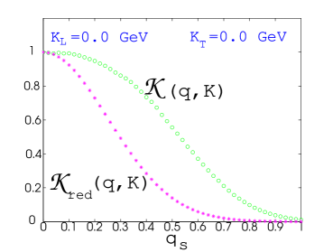
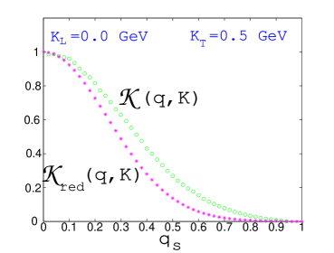
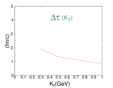
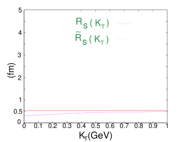
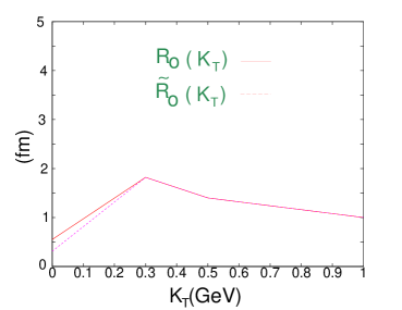
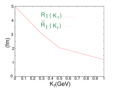
Figure 1: First two panels: The correlation function in side-direction ($q_{o}{\,=\,}q_{l}{\,=\,}0$) for pairs with $K_{\rm L}{\,=\,}0$ (such that the $R_{ol}$ cross term vanishes $\!{}^{{\bf?}}$) and $K_{\rm T}{\,=\,}0$ and 0.5 GeV, respectively. Third panel: The emission time duration $\Delta\tau{\,=\,}\sqrt{R_{o}^{2}-R_{s}^{2}}/\beta_{\rm T}$ as a function of $K_{\rm T}$ for $K_{\rm L}{\,=\,}0$. Second row: $R_{s}$, $R_{o}$, and $R_{l}$ as functions of $K_{\rm T}$ for $K_{\rm L}{\,=\,}0$. We checked that the HBT radii correctly reproduce the rms widths of the space-time scatter plots of the produced pions in the appropriate 0 $\textstyle K$-windows.

Ackowledgement: This work was supported by the Deutsche Forschungsgemeinschaft.

References

References

• [1] This is reviewed in U.A. Wiedemann and U. Heinz, Phys. Rep. 319, 145 (1999), and U. Heinz and B.V. Jacak, Ann. Rev. Nucl. Part. Sci. 49, 529 (1999), where many references to the original papers can be found.
• [2] Q.H. Zhang, P. Scotto, and U. Heinz, Phys. Rev. C 58, 3757 (1998); U. Heinz, P. Scotto, and Q.H. Zhang, CERN-TH/2000-123.
• [3] S. Chapman, P. Scotto, and U. Heinz, Heavy Ion Phys. 1, 1 (1995); S. Pratt, Phys. Rev. C 56, 1095 (1997).
• [4] B. Tomášik, U.A. Wiedemann, and U. Heinz, nucl-th/9907096.
• [5] L. Lönnblad and T. Sjöstrand, Phys. Lett. B 351, 293 (1995), and Eur. Phys. J. C 2, 165 (1998); B. Andersson and M. Ringner, Nucl. Phys. B513, 627 (1998), and Phys. Lett. B 421, 283 (1998); K. Fialkowski and R. Wit, Eur. Phys. J. C 2, 691 (1998); Phys. Lett. B 438, 154 (1998); hep-ph/9810492; K. Fialkowski, R. Wit, and J. Wosiek, Phys. Rev. D 58, 094013 (1998).
• [6] K. Geiger, J. Ellis, U. Heinz, and U.A. Wiedemann, Phys. Rev. D 61, 054002 (2000).
• [7] S. Todorovova, private communication.
• [8] Q.H. Zhang, U.A. Wiedemann, C. Slotta, and U. Heinz, Phys. Lett. B 407, 33 (1997).