How to Renormalize the Gap Equation
in High Density QCD

Abstract

We discuss two technical issues related to the gap equation in high-density QCD: i) how to obtain the asymptotic solution with well controlled approximations, and ii) the renormalization of four-quark operators in the high-density effective field theory.

Recently Son obtained the leading exponential behavior of the superconducting gap in QCD at asymptotically high density using both an indirect renormalization group argument and a direct QCD calculation[1]. Subsequently many papers confirmed Son’s result[2, 3, 4]. However, to the best of our knowledge, the analytical determinations of the gap suffer from two flaws. First, the gap equation is divergent and so must be regularized and renormalized. Most treatments have taken the baryon density as a sharp cutoff. This might cause some concern since it leads to the possibility of contaminating the low energy physics of the gap with ad hoc high energy physics. Issues of cutoff sensitivity have been addressed in Ref. [3] and Ref. [4]. Second, the solution of the gap equation at momenta large compared to the gap has been obtained by assuming (what appears to be) a particularly unhealthy approximation which allows the integral equation for the gap to be expressed as a simple differential equation. The goals of this paper are modest. Using cutoff regularization we define a renormalized gap equation and we find the exact asymptotic solution, thus excising the flaws contained in previous determinations. Our results confirm Son’s original analysis. We also obtain the asymptotic solution using dimensional regularization with minimal subtraction.

Many degrees of freedom, including antiparticles and hard gluons, are not dynamical on the Fermi surface. Hence it is sensible to work with an effective theory of QCD appropriate to the scales in question. Explicit construction of the effective field theory appropriate for momentum scales below $2\mu$, can be found in papers by Hong[5]. The fermions in this effective theory live on the two-dimensional Fermi surface and so depend only on the parallel momentum, $q_{\parallel}$. The gluons on the other hand propagate in directions perpendicular to the Fermi surface as well and therefore also depend on the perpedicular momentum, $q_{\perp}$. Hence we should treat the effective field theory as a superposition of two-dimensional theories, one for each direction on the Fermi surface, interacting through four-dimensional gluons and contact operators. Only the graphs shown in Fig. (1a) and (1b) need be calculated if we are interested in the leading exponential behavior of the gap. The sum of these graphs is (after rotating to Euclidean space)

$${\Delta}(p_{\parallel}) = \int{{d^{2}{q_{\parallel}}}\over(2\pi)^{2}}{{\Delta}(q_{\parallel})\over{q_{\parallel}^{2}+{\Delta}(q_{\parallel})^{2}}}\Bigg{\{}{{2g^{2}}\over 3}\int{{d^{2}{q_{\perp}}}\over(2\pi)^{2}}\left({1\over{{\vec{q}}_{\perp}^{\;2}+{{\pi\over 4}M_{{\scriptscriptstyle}d}^{2}|p_{{\scriptscriptstyle}0}-q_{{\scriptscriptstyle}0}|/|{{\vec{q}}_{\perp}}\;|}}}+{1\over{{\vec{q}}_{\perp}^{\;2}+{M_{{\scriptscriptstyle}d}^{2}}}}\right)+{\tilde{D}}\Bigg{\}},$$ (1)

where the propagators within the parentheses represent magnetic and electric gluon exchanges, respectively, and

$$M_{{\scriptscriptstyle}d}^{2}={{{N_{f}}g^{2}\mu^{2}}\over{2\pi^{2}}}.$$ (2)

The effects of hard gluon exchange, antiparticle exchange and any residual gauge dependence are represented by the coefficient, $\tilde{D}$, of a four-fermi operator in the two-dimensional effective theory.

It is clear that the integration over $q_{\perp}$ is divergent. We will first regulate the gap equation with a sharp cutoff, $\Lambda_{\perp}$. In principle there is a cutoff associated with the parallel integration as well and therefore in general we have ${\tilde{D}}={\tilde{D}}(\Lambda_{\perp},\Lambda_{{\parallel}})$. It is straightforward to do the integration over $q_{\perp}$ and ${\vec{q}}_{\parallel}$. We obtain

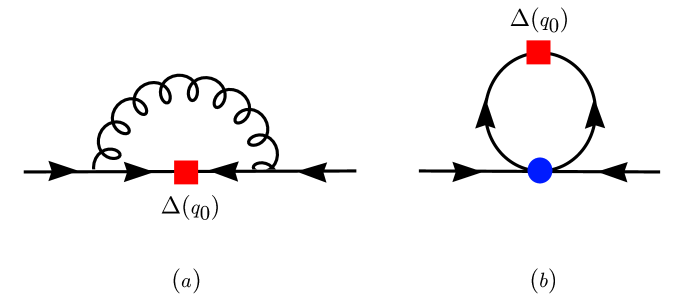
FIG. 1.: The leading diagrams contributing to the gap equation. The solid square denotes the gap, $\Delta$, while the solid circle denotes an insertion of the counterterm, $\tilde{D}$.

$${\Delta}(p_{{\scriptscriptstyle}0}) = {1\over 2}{{\cal C}^{2}}{\int_{-\Lambda_{{\parallel}}}^{\Lambda_{{\parallel}}}}{d{q_{{\scriptscriptstyle}0}}}{{\Delta}(q_{{\scriptscriptstyle}0})\over\sqrt{q_{{\scriptscriptstyle}0}^{2}+{\Delta}(q_{{\scriptscriptstyle}0})^{2}}}\left(\log{{\cal M}_{{\scriptscriptstyle}\Lambda_{\perp}}\over|p_{{\scriptscriptstyle}0}-q_{{\scriptscriptstyle}0}|}+{{\scriptscriptstyle}1\over 2}D(\Lambda_{\perp},\Lambda_{{\parallel}})\right)$$ (3)

where

$${\cal M}_{{\scriptscriptstyle}\Lambda_{\perp}}={{4(\Lambda_{\perp})^{6}}\over{\pi M_{{\scriptscriptstyle}d}^{5}}};\qquad{\tilde{D}}={{g^{2}D}\over{18\pi}};\qquad{\cal C}={g\over{3\sqrt{2}\pi}}.$$ (4)

Since ${\Delta}(p_{{\scriptscriptstyle}0})$ is independent of the cutoff, $D$ runs according to

$${D}(\Lambda_{\perp},\Lambda_{{\parallel}})={D}(\eta,\Lambda_{{\parallel}})-6\log{{{\Lambda_{\perp}^{2}}\over{\eta^{2}}}}.$$ (5)

Naive dimensional analysis suggests that ${D}(\Lambda_{\perp}={2\mu},\Lambda_{{\parallel}})$ is small and can therefore be dropped at leading order. The effect of the running of $D$ appears at next order  [4]. We then have

$${\cal M}_{{\scriptscriptstyle}2\mu}={{2^{10}\sqrt{2}\pi^{4}\mu}\over{{N_{f}}^{5/2}g^{5}}};\qquad{D}(2\mu,\Lambda_{{\parallel}})={D}(\Lambda_{{\parallel}}).$$ (6)

Dropping all subscripts for simplicity the gap equation becomes

$${\Delta}(p) = {1\over 2}{{\cal C}^{2}}{\int_{0}^{\Lambda}}{d{q}}{{\Delta}(q)\over\sqrt{q^{2}+{\Delta}(q)^{2}}}\left(\log{{\cal M}^{2}\over|p^{2}-q^{2}|}+D(\Lambda)\right).$$ (7)

Because of the log singularity at $q\sim p$, the integral is dominated by momenta $q\sim p$. Therefore in the asymptotic region defined by $p\gg{\Delta}(p)$, we can take $q\gg{\Delta}(q)$ under the integral. Hence asymptotically the gap equation becomes the homogeneous integral equation

$${\Delta}(p) = {1\over 2}{{\cal C}^{2}}{\int_{\Delta}^{\Lambda}}{{d{q}}\over q}{\Delta}(q)\left(\log{{\cal M}^{2}\over|p^{2}-q^{2}|}+D(\Lambda)\right).$$ (8)

Note that although the integral equation is homogeneous, we have by necessity introduced an infrared cutoff, $\Delta$, which we will see is related to the overall normalization of the gap. In order to proceed, consider the derivative of the gap equation:

$${\Delta}^{\prime}(p) = {{\cal C}^{2}}p{\int_{\Delta}^{\Lambda}}{{d{q}}\over q}{{{\Delta}(q)}\over{(q^{2}-p^{2})}}.$$ (9)

Note that since the counterterm is no longer present, this integral is convergent as $\Lambda\rightarrow\infty$.

We make an ansatz of the form ${\Delta}(p)=p^{z}$ with $z$ a complex number. Inserting this solution in eq. (9) leads to the indicial equation:

$$z = {{\cal C}^{2}}p^{{\scriptscriptstyle}2-z}{\int_{\Delta}^{\Lambda}}{{d{q}}}{q^{{\scriptscriptstyle}z-1}\over{(q^{2}-p^{2})}}.$$ (10)

The integral is straightforward to evaluate. It is given by

$${\it Re}{1\over{1-\exp{2\pi i(z-1)}}}{\oint}{{d{q}}}{q^{{\scriptscriptstyle}z-1}\over{(q^{2}-p^{2}+i\epsilon)}},$$ (11)

where the contour in the complex q-plane is taken to enclose the poles at $p-i\epsilon$ and $-p+i\epsilon$ while avoiding the branch point at the origin. For ${\Delta}\ll p\ll\Lambda$ we can take the limits ${\Delta}\rightarrow 0$ and $\Lambda\rightarrow\infty$ since the corrections are suppressed by powers of $p/\Lambda$ and ${\Delta}/p$. The resulting indicial equation is transcendental

$$z = {-{\pi\over 2}}{{\cal C}^{2}}\cot{{\pi z}\over 2}.$$ (12)

Therefore the exact asymptotic solution of the gap equation is $p^{z}$ with z satisfying eq. (12). For small z this has the solution

$$z=\pm i{\cal C}.$$ (13)

The general asymptotic solution to the gap equation in the weak coupling limit can then be written as

$${\Delta}(p)=A\sin{({\cal C}\log{\Lambda^{*}\over p})},$$ (14)

where the constants $A$ and $\Lambda^{*}$ are to be determined.

We will now determine the constant $A$. In the region ${\Delta}\leq p<2\mu$, ${\Delta}(p)$ has one maximum, which we will assume is at $p={\bar{\Delta}}$ with ${\Delta}\leq{\bar{\Delta}}<\Lambda$. This determines $A={{\Delta}({\bar{\Delta}})}$. We can find ${\bar{\Delta}}$ by plugging the general solution, eq. (14), into eq. (9) which leads to the equation

$$0={\Delta}^{\prime}(p)|_{p={\bar{\Delta}}}={{\cal C}^{2}}{\bar{\Delta}}\;{{\Delta}({\bar{\Delta}})}{\int_{\Delta}^{\Lambda}}{{d{q}}\over q}\sin{({\cal C}\log{\Lambda^{*}\over q})}{1\over{(q^{2}-{\bar{\Delta}}^{2})}}.$$ (15)

A straightforward computation then gives

$$\cos{x_{{\scriptscriptstyle}{\Delta}}}+\sum_{n=1}^{\infty}{1\over{({\cal C}^{2}+4n^{2})}}({\cal C}^{2}\left[\exp{\left({n\over{\cal C}}(\pi-2{x_{{\scriptscriptstyle}{\Delta}}})\right)}\cos{x_{{\scriptscriptstyle}{\Delta}}}+\exp{\left(-{n\over{\cal C}}(\pi-2{x_{{\scriptscriptstyle}\Lambda}})\right)}\cos{x_{{\scriptscriptstyle}\Lambda}}\right]$$ (16)

$$+2{\cal C}n\left[\exp{\left({n\over{\cal C}}(\pi-2{x_{{\scriptscriptstyle}{\Delta}}})\right)}\sin{x_{{\scriptscriptstyle}{\Delta}}}-\exp{\left(-{n\over{\cal C}}(\pi-2{x_{{\scriptscriptstyle}\Lambda}})\right)}\sin{x_{{\scriptscriptstyle}\Lambda}}\right])=0$$ (17)

where

$${x_{{\scriptscriptstyle}{\Delta}}}={\cal C}\log{\Lambda^{*}\over{{\Delta}}};\qquad{x_{{\scriptscriptstyle}\Lambda}}={\cal C}\log{\Lambda^{*}\over{\Lambda}}.$$ (18)

The expression under the sum is exponentially suppressed in the QCD coupling $g$. Therefore, to leading order $x_{{\scriptscriptstyle}{\Delta}}=\pi/2$ and we can identify ${\bar{\Delta}}$ with ${{\Delta}}$. This determines $A={{\Delta}}({\Delta})$ and the asymptotic solution is

$${\Delta}(p)={{\Delta}}({\Delta})\sin{({\cal C}\log{\Lambda^{*}\over p})};\qquad\qquad{\Delta}({\Delta})={\Delta}=\Lambda^{*}\exp{\left(-{\pi\over{2{\cal C}}}\right)}.$$ (19)

We now determine $\Lambda^{*}$. We can rewrite eq. (8) as

$${\Delta}(p) = {1\over 2}{{\cal C}^{2}}{\int_{\Delta}^{\Lambda}}{{d{q}}\over q}{\Delta}(q)\log{{\bar{\cal M}}^{2}\over|p^{2}-q^{2}|}+{1\over 2}{{\cal C}^{2}}\left(D(\Lambda)-D({\bar{\cal M}})\right){\int_{\Delta}^{\Lambda}}{{d{q}}\over q}{\Delta}(q)$$ (20)

where

$${\bar{\cal M}}^{2}={\cal M}^{2}\exp{(D({\bar{\cal M}}))}.$$ (21)

The condition that ${\Delta}(p)$ be independent of the choice of cutoff leads to the renormalization group equation

$$\Lambda{d\over{d\Lambda}}\left(D(\Lambda)-D({\bar{\cal M}})\right)=-{\cal C}\tan({\cal C}\log{{\Lambda^{*}}\over\Lambda})\left[\left(D(\Lambda)-D({\bar{\cal M}})\right)+\log{{{{\bar{\cal M}}^{2}}\over{\Lambda^{2}}}}\right]$$ (22)

where we have used the asymptotic solution, eq. (19). The solution of this equation is

$$D(\Lambda)-D({\bar{\cal M}})={2\over{\cal C}}\left[\tan({\cal C}\log{{\Lambda^{*}}\over\Lambda})-{\sin({\cal C}\log{{{\Lambda^{*}}\over{\bar{\cal M}}}})\over\cos({\cal C}\log{{\Lambda^{*}}\over\Lambda})}\right]-\log{{{{\bar{\cal M}}^{2}}\over{\Lambda^{2}}}}.$$ (23)

Notice that the difference between counterterms evaluated at different choices of scale is of order $g^{2}$. The counterterm has a strong cutoff dependence except when $\Lambda\sim{{\bar{\cal M}}}$. The peculiar running of the counterterm is very similar to the running of a counterterm which arises at leading order in effective field theory treatments of the three-body problem in nuclear physics[6].

Choosing $\Lambda={{\bar{\cal M}}}$, the renormalized gap equation is

$${\Delta}(p) = {1\over 2}{{\cal C}^{2}}{\int_{0}^{{{\bar{\cal M}}}}}{d{q}}{{\Delta}(q)\over\sqrt{q^{2}+{\Delta}(q)^{2}}}\log{{{\bar{\cal M}}}^{2}\over|p^{2}-q^{2}|}.$$ (24)

We can now find $\Lambda^{*}$ by plugging the general solution, eq. (19), into the asymptotic form of the renormalized gap equation, eq. (24), evaluated at $p=\Lambda^{*}$. We then have

$$0={\Delta}({\Lambda^{*}})={1\over 2}{{\cal C}^{2}}{{\Delta}({{\Delta}})}{\int_{\Delta}^{\bar{\cal M}}}{{d{q}}\over q}\sin{({\cal C}\log{\Lambda^{*}\over q})}\log{{{\bar{\cal M}}}^{2}\over|{\Lambda^{*}}^{2}-q^{2}|}.$$ (25)

A straightforward computation then gives

$$0=\sin{x_{{\scriptscriptstyle}{\bar{\cal M}}}}-2{x_{{\scriptscriptstyle}{\bar{\cal M}}}}\cos{x_{{\scriptscriptstyle}{\bar{\cal M}}}}+{1\over 2}\sum_{n=1}^{\infty}{1\over n}{1\over{({\cal C}^{2}+4n^{2})}}({\cal C}^{3}\exp{\left({2n{x_{{\scriptscriptstyle}{\bar{\cal M}}}}\over{\cal C}}\right)}\cos{x_{{\scriptscriptstyle}{\bar{\cal M}}}}$$ (26)

$$-2{\cal C}^{2}\left[\exp{\left({2n{x_{{\scriptscriptstyle}{\bar{\cal M}}}}\over{\cal C}}\right)}\sin{x_{{\scriptscriptstyle}{\bar{\cal M}}}}+n\exp{\left({-n\pi\over{\cal C}}\right)}\right])$$ (27)

where

$${x_{{\scriptscriptstyle}{\bar{\cal M}}}}={\cal C}\log{\Lambda^{*}\over{{\bar{\cal M}}}}.$$ (28)

The expression under the sum is exponentially suppressed in the QCD coupling $g$. Therefore, to leading order ${x_{{\scriptscriptstyle}{\bar{\cal M}}}}=0$ and we can identify $\Lambda^{*}={\bar{\cal M}}$.

The final form for the asymptotic solution is thus

$${\Delta}(p)={{\Delta}}({\Delta})\sin{({\cal C}\log{{\bar{\cal M}}\over p})},$$ (29)

and the gap is

$${{\Delta}}={{\bar{\cal M}}}\exp{\left(-{\pi\over{2{\cal C}}}\right)}={{2^{10}\sqrt{2}\pi^{4}\mu}\over{{N_{f}}^{5/2}g^{5}}}\;\exp{\left({D({2\mu},{{\cal M}})\over 2}\right)}\;\exp{\left(-{3\pi^{2}\over{\sqrt{2}{g}}}\right)}.$$ (30)

This is Son’s result[1] aside from the additional contribution to the prefactor from the counterterm, which is expected to be a number of order one.

One may wonder whether use of cutoff regularization in dense QCD violates important symmetries. Consistent implementation of dimensional regularization would erase these concerns. We will see that dimensional regularization with minimal subtraction is a quick way of obtaining the asymptotic solution directly from the gap equation. We can continue the four-dimensional measure to an $2+n$-dimensional measure

$$\int{{d^{2}q_{\parallel}}\over(2\pi)^{2}}\int{{d^{n}q_{\perp}}\over(2\pi)^{n}}.$$ (31)

The gap equation relevant to dimensional regularization with minimal subtraction is

$${\Delta}(p_{\parallel}) = \int{{d^{2}{q_{\parallel}}}\over(2\pi)^{2}}{{\Delta}(q_{\parallel})\over{q_{\parallel}^{2}+{\Delta}(q_{\parallel})^{2}}}\Bigg{\{}{{2g^{2}}\over 3}\int{{d^{n}{q_{\perp}}}\over(2\pi)^{n}}\left({1\over{{\vec{q}}_{\perp}^{\;2}+{{\pi\over 4}M_{{\scriptscriptstyle}d}^{2}|p_{{\scriptscriptstyle}0}-q_{{\scriptscriptstyle}0}|/|{{\vec{q}}_{\perp}}\;|}}}+{1\over{{\vec{q}}_{\perp}^{\;2}+{M^{2}}}}\right)+{\tilde{D}}^{{{\scriptscriptstyle}\overline{MS}}}\Bigg{\}}.$$ (32)

The integrals of the gluon propagators in $n$-dimensions are

$$\int{{d^{n}{q_{\perp}}}\over(2\pi)^{n}}\;{1\over{{\vec{q}}_{\perp}^{\;2}+{A/|{\vec{q}}\;|}}}\;=\;{1\over{6\pi}}\left({{\lambda^{3}}\over A}\right)^{\epsilon}\;{{\Gamma\left(\epsilon\right)\Gamma\left(1-\epsilon\right)}\over{\Gamma\left(1-{{3\epsilon}\over 2}\right)}};$$ (33)

$$\int{{d^{n}{q_{\perp}}}\over(2\pi)^{n}}\;{1\over{{\vec{q}}_{\perp}^{\;2}+{M^{2}}}}\;=\;{1\over{6\pi}}\left({{\lambda^{3}}\over{M^{3}}}\right)^{\epsilon}\;\Gamma\left({{3\epsilon}\over 2}\right),$$ (34)

where $\epsilon=(2-n)/3$ and $\lambda$ is a renormalization scale. Absorbing the $1/\epsilon$ pole into the counterterm, we can then define the regularized gap equation

$${\Delta}(p) = {1\over 2}{{\cal C}^{2}}{\int_{0}^{\infty}}{d{q}}{{\Delta}(q)\over\sqrt{q^{2}+{\Delta}(q)^{2}}}\left(\log{{\cal M}_{\lambda}^{2}\over|p^{2}-q^{2}|}+D^{{\scriptscriptstyle}\overline{MS}}(\lambda)\right)$$ (35)

where

$${\cal M}_{{\scriptscriptstyle}\lambda}={{4(\lambda)^{6}}\over{\pi{M_{{\scriptscriptstyle}d}}^{5}}};\qquad{\tilde{D}}^{{\scriptscriptstyle}\overline{MS}}={{g^{2}D^{{\scriptscriptstyle}\overline{MS}}}\over{18\pi}}.$$ (36)

This equation was obtained in Ref. [4]. The counterterm runs according to

$${D^{{\scriptscriptstyle}\overline{MS}}}(\lambda)={D^{{\scriptscriptstyle}\overline{MS}}}(\eta)-6\log{{{{\lambda}^{2}}\over{{\eta}^{2}}}}.$$ (37)

Physical quantities are $\lambda$-independent so we choose $\lambda=2\mu$. We again consider the asymptotic gap equation

$${\Delta}(p) = {1\over 2}{{\cal C}^{2}}{\int_{{\Delta}}^{\infty}}{d{q}}{{\Delta}(q)\over q}\left(\log{{\cal M}_{2\mu}^{2}\over|p^{2}-q^{2}|}+D^{{\scriptscriptstyle}\overline{MS}}(2\mu)\right).$$ (38)

Say the asymptotic solution is of the form ${\Delta}(p)=p^{z}$. All scales then appear multiplied by power law divergences which vanish in minimal subtraction. Hence it is appropriate to return to the unsubtracted expression for the log in eq. (34). We then obtain

$$p^{z}={{\cal C}^{2}}\Gamma(\epsilon){\int_{0}^{\infty}}{{d{q}}}{q^{{\scriptscriptstyle}z-1}\over{(q^{2}-p^{2})^{\epsilon}}}.$$ (39)

Again this integral is straightforward to evaluate and leads to

$$p^{z}={{\cal C}^{2}}\Gamma(\epsilon)\left[{{p^{z-2\epsilon}}\over 2}\cos{\pi(\epsilon-{z\over 2})}{{\Gamma\left(\epsilon-{z\over 2}\right)\Gamma\left({z\over 2}\right)}\over\Gamma\left(\epsilon\right)}\right],$$ (40)

which as expected reduces to

$$z={-{\pi\over 2}}{{\cal C}^{2}}\cot{{\pi z}\over 2}$$ (41)

in the limit $\epsilon\rightarrow 0$. Notice that the original $\Gamma(\epsilon)$ pole from the integration over perpendicular momenta cancels a $1/\Gamma(\epsilon)$ zero from the integration over $q$. The asymptotic solution is again

$${\Delta}(p)={{\Delta}}({\Delta})\sin{({\cal C}\log{\Lambda^{*}\over p})},$$ (42)

where the prefactor is fixed by the argument presented above. Now fixing $\Lambda^{*}$ is trivial since there is only one scale in the problem. We have

$$\Lambda^{*}={{\cal M}_{2\mu}}\exp{{D^{{\scriptscriptstyle}\overline{MS}}(2\mu)}\over 2}$$ (43)

from which follows

$${{\Delta}}={{2^{10}\sqrt{2}\pi^{4}\mu}\over{{N_{f}}^{5/2}g^{5}}}\;\exp{\left({{D^{{\scriptscriptstyle}\overline{MS}}(2\mu)}\over 2}\right)}\;\exp{\left(-{3\pi^{2}\over{\sqrt{2}{g}}}\right)}.$$ (44)

Evidently the counterterm does not depend on the renormalization scale in the longitudinal direction in minimal subtraction. As argued previously, the counterterm is of order $g^{{\scriptscriptstyle}0}$ and can be dropped at this order in the expansion.

We thank Martin Savage for valuable conversations. This work is supported in part by the U.S. Dept. of Energy under Grants No. DE-FG03-97ER4014 and DOE-ER-40561.