Isovector and Isoscalar superfluid phases in rotating nuclei

Abstract

The subtle interplay between the two nuclear superfluids, isovector T=1 and isoscalar T=0 phases, are investigated in an exactly soluble model. It is shown that T=1 and T=0 pair-modes decouple in the exact calculations with the T=1 pair-energy being independent of the T=0 pair-strength and vice-versa. In the rotating-field, the isoscalar correlations remain constant in contrast to the well known quenching of isovector pairing. An increase of the isoscalar (J=1, T=0) pair-field results in a delay of the bandcrossing frequency. This behaviour is shown to be present only near the N=Z line and its experimental confirmation would imply a strong signature for isoscalar pairing collectivity. The solutions of the exact model are also discussed in the Hartree-Fock-Bogoliubov approximation.

PACS numbers : 21.60.Cs, 21.10.Hw, 21.10.Ky, 27.50.+e

There is overwhelming evidence that the isovector, T=1 pairing field among identical nucleons is an essential component of the nuclear mean-field potential. The bulk of nuclear ground-state properties, like the odd-even mass differences and the moments of inertia of deformed nuclei can be accounted for by considering nucleons to be in a superfluid (T=1, J=0) paired-phase[1]. These effects have been studied mostly in heavier nuclei with N$>$Z, where the Fermi surfaces of protons and neutrons lie in different major shells.

In recent years, however, due to a substantial progress achieved in the sensitivity of the detecting systems it has been possible to study nuclei near the N$=$Z line in the mass A$=$70 and 80 regions. Furthermore, with the availability of radioactive beams these studies are expected to reach even heavier N$=$Z nuclei. For these nuclei, one expects the pairing between protons and neutrons to become important, since the Fermi surfaces of both protons and neutrons lie in the same major shell.

The role of the isovector T=1 pairing between protons and neutrons in the low-spin regime has been discussed in recent studies by [2, 3]. The importance of the isoscalar T=0 pairing can be inferred from masses[7] and studies of high-spin states[4, 5, 6]. However, most of these studies are based on the mean-field approximation which predict a transitional behaviour for rotating nuclei for the T=1 and T=0 pair-fields as a function of the rotational frequency and the strength of the T=0 interaction[7].

The purpose of the present study is to examine properties of the isoscalar and isovector correlations within an exactly soluble model of a deformed sinlge-j shell and to compare to the predictions of the mean-field HFB approximation. The observable consequences of the T=0 pair-field which have remained illusive are also discussed in the present study.

The model hamiltonian consists of a cranked deformed one-body term and a scalar two-body interaction[8, 9]

$$H^{\prime}=h^{\prime}+V_{2},$$ (1)

where,

$$h^{\prime}=h_{def}-\omega J_{x},$$ (2)

with

$$h_{def}=-4\kappa{\sqrt{4\pi\over 5}}\sum_{ij}<j|Y_{20}|i>\delta_{\tau_{i}\tau_{j}}\delta_{m_{i}m_{j}}c^{\dagger}_{j}c_{i}.$$ (3)

The labels $i,j,...$ denote the magnetic quantum-number ($m$) of the j- shell and the isospin projection quantum-number $\tau$ [$\tau$=1/2 (neutron) and -1/2(proton)]. The deformation energy $\kappa$ is equal to the usual deformation parameter $\beta$ by $\kappa=0.16\hbar\omega(N+3/2)\beta$ in units of G (ref. [10]). The two-body interaction in Eq. 1 is given by

$$V_{2}={\frac{1}{2}}\sum_{JMTT_{z}}E_{JT}A_{JM;TT_{z}}^{\dagger}A_{JM;TT_{z}},$$ (4)

with $A_{JM;TT_{z}}^{\dagger}=(c_{j{1\over 2}}^{\dagger}c_{j{1\over 2}}^{\dagger})_{JM;TT_{z}}$ and $A_{JM;TT_{z}}=(A_{JM;TT_{z}}^{\dagger})^{\dagger}$. For the antisymmetric-normalized two-body matrix-element ($E_{JT}$), we use the delta-interaction which for a single j-shell is given by [11]

$$E_{JT}=-G{\frac{(2j+1)^{2}}{2(2L+1)}}\left\{\left[\begin{array}[]{ccc}j{}&~{}j{}&J\\ \frac{1}{2}{}&-\frac{1}{2}&0\end{array}\right]^{2}+{1\over 2}\{1+(-1)^{T}\}\left[\begin{array}[]{ccc}j{}&j{}&J\\ \frac{1}{2}{}&\frac{1}{2}{}&1\end{array}\right]^{2}\right\}$$ (5)

where the bracket $[~{}~{}]$ denotes the Clebsch-Gordon coefficient.

As mentioned in the introduction, one of the objectives of the present work is to investigate the HFB approximation. In the following, we present some basic HFB formulae, for details see for instance ref.[12]. The HFB equations are given by

$${\cal H}^{\prime}\left(\begin{array}[]{c}U\\ V\end{array}\right)=E^{\prime}_{i}\left(\begin{array}[]{c}U\\ V\end{array}\right),$$ (6)

where

$${\cal H}^{\prime}= \left(\begin{array}[]{cc}h^{\prime}{}{}{}&\Delta\\ -\Delta^{\ast}{}{}{}&-(h^{\prime})^{\ast}\end{array}\right).$$ (9)

with

$$h^{\prime}_{ij} = \epsilon^{\prime}_{ij}+\Gamma_{ij},$$ (10)

$$\epsilon^{\prime}_{ij} = <i|h_{def}|j>-(\lambda_{p}Z+\lambda_{n}N+\omega m_{i})\delta_{ij},$$ (11)

$$\Gamma_{ij} = \sum_{kl}<ik|v_{a}|jl>\rho_{lk},$$ (12)

$$\Delta_{ij} = {1\over 2}\sum_{kl}<ij|v_{a}|kl>\kappa_{kl}.$$ (13)

$$\rho=V^{\ast}V^{T},\quad\quad\kappa=V^{\ast}U^{T}=-UV^{\dagger}.$$ (14)

In order to evaluate the angular-momentum dependence of the pair-energy, we define the coupled pair-field through

$$\Delta_{ij}=\sum_{JMTT_{z}}\left[\begin{array}[]{ccc}j{}{}&j{}{}&J\\ m_{i}{}{}&m_{j}{}{}&M\\ \end{array}\right]\left[\begin{array}[]{ccc}{1\over 2{}{}}&{1\over 2{}{}}&T\\ \tau_{i}{}{}&\tau_{j}{}{}&T_{z}\\ \end{array}\right]\Delta_{JT},$$ (19)

with

$$\Delta_{JT}=E_{JT}\sum_{ij}$$ (20)

$$\left[\begin{array}[]{ccc}j{}&j{}&J\\ m_{i}{}&m_{j}{}&m_{i}+m_{j}\\ \end{array}\right]\left[\begin{array}[]{ccc}{1\over 2}&{1\over 2}&T\\ \tau_{i}&\tau_{j}&\tau_{i}+\tau_{j}\\ \end{array}\right]\kappa_{ij}.$$ (25)

The pair-energy can now be expressed in terms of the coupled pair-fields as

$$E_{pair}={1\over 2}\sum_{JT}{\Delta_{JT}\Delta_{JT}^{*}\over E_{JT}}.$$ (26)

The above expression is quite useful since in the exact calculations there is no gap parameter $\Delta$, but one may associate “$E_{pair}$” with the expectation value of the two-body residual interaction, $V_{2}$, Eq.4 To obtain the $\Delta$-value from the exact analysis, Eq.26 is then simply inverted.

The HFB solutions have been obtained by solving the Eqs. (6-14) self-consistently. In order to treat both the T=0 and the T=1 pair-fields simultaneously, it is necessary to define complex HFB potentials, since the symmetries of the T=1 and T=0 n-p fields are different[13]. The initial complex HFB wavefunctions have been constructed by using the expressions for real and imaginary $V$’s and $U$’s of the HFB transformation in terms of the pair-gaps[13]. We would like to mention that no symmetry restrictions have been imposed on the HFB wavefunction since it is known that symmetries lead to exclusion of particular correlations. For more details concerning the HFB-transformation in the presence of both T=1 and T=0 pairing, we refere the reader to refs. [14, 15].

FIG. 1.: The exact single-j shell model pairing-gaps as a function of the T=0 strength for a system with 2-protons and 2-neutrons in $f_{7/2}$ shell.

Several mean-field studies show that the T=0 and T=1 pairing-modes are exclusive in the BCS-approximation[7, 16]. The system is always choosing the mode that generates the lowest energy, which in the case of equal weight for each pair results in either T=0 and T=1 pairing[6]. In the presence of approximate particle-number projection, the two modes coexist, but only above a critical strength[6, 7]. Using a more complex model space also results in the possibility of mixed solutions[5, 15]. The question, therefore, arises whether the exclusiveness is persistent in an exact model. Fig. 1 shows the size of the T=1 correlations as a function of increasing T=0 strength in the exact analysis. The figure clearly shows that the two modes are essentially independent. There is no critical strength for either pairing mode and therefore one expects to have both modes present in nuclei. From this we can conclude that the exclusion between the two modes is a mean-field effect. It also implies that atomic nuclei exhibit the unique possibility of exhibiting two different pairing condensates simultanously.

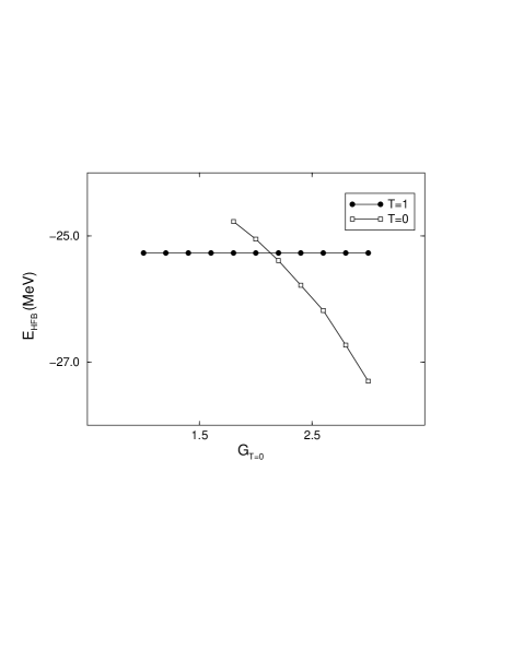
FIG. 2.: The HFB pairing energy for 4-protons and 4-neutrons as a function of the T=0 strength.

In order to explore further the mutual exclusiveness of the T=1 and T=0 pair-fields obtained in earlier studies, we have studied the HFB solution as a function of the strength of the T=0 interaction. The results are presented in Fig. 2. For the normal strength $G_{T=0}=1$, the solution corresponds to a T=1 pair-field. With increasing $G_{T=0}$ the HFB energy remains constant which is obvious since the solution has only the T=1 component and there is no T=0 component. The T=0 solution shown in Fig. 2 has been obtained by solving the HFB equations for a very large value of $G_{T=0}$ ($G_{T=0}=2.8$) and then using this solution for lower values of $G_{T=0}$. In this manner, it was possible to obtain a T=0 solution also below the critical point, see Fig. 2. We note from Fig. 2 that the two solutions coexist for most of the $G_{T=0}$ values. They represent two different solutions of the HFB equations.

The exact solution, presented in Figs. 1 contains both the T=0 and T=1 pair-modes, whereas HFB gives two separate solutions, corresponding to either T=0 or T=1 pair-fields. The difference between the two models resides in the fact that in the exact model, the two-body interaction always is a scalar whereas in the HFB-aproximation, the pairing potential is either a T=0 or T=1 field, with the corresponding symmetry. Our analysis shows that starting from a certain solution, with a given symmetry, this symmetry propagates to the next solution (with different $G_{T=0}$), analoguous to other self-consistent symmetries of the HFB hamiltonian, see e.g. the discussion in [14]. The different pair-fields appear as independent of each other. Our results further indicate, that for a certain strength of the $G_{T=0}$ pair field, energy can be gained. This conforms with earlier results to associate the Wigner energy with T=0 pair correlations[7].

FIG. 3.: Behaviour of the exact shell model pair-gaps as a function of rotational frequency $\hbar\omega$ for 2+2 particles in the $f_{7/2}$ shell. The solid (dashed) lines represent the T=1 (T=0) part of the pairing-energy. For the case of T=0, we show all individual components of the force, clearly demonstrating the importance of the different $J$’s. In contrast, the T=1 force is dominated by the J=0 component.

As a next step, we consider the response of the nuclear pair-potential to the rotating fields. In Fig. 3, we show the total pair-field (Eq. 15) as well as selected individual $(J,~{}T)$ contribution as a function of the rotational frequency ( $\hbar\omega$ ) for 4 particles (2 protons and 2 neutrons) in the $f_{7/2}$ shell. First of all, we may note the distinct difference between the T=1 and T=0 pairing fields. Whereas the T=1 field is dominated by one component with J=0, the T=0 mode is dominated by the J=1 and $J=2j$ part of the interaction, also the intermediate spins $J=3,~{}5$ play a role. This already indicates that a discussion of a pairing force restricted to $L=0$ may be appropriate for the T=1 part of the interaction, but not for T=0, see also ref. [17, 18].

As we increase the rotational frequency, the T=1 pairing-correlations (solid line) reveal the well known drop due to particle-alignment from the $f_{7/2}$-shell at around $\hbar\omega=0.7G$. At this crossing point, the yrast band changes character from the paired $(J=0)$ configuration to the aligned $(J=M_{x}=6+6)$ state.

Similar calculations were performed also for the case of the (4+2) and (4+4) systems. Qualitatively, they all show the same trend, where of course the size of the drop in correlation energy depends on the number of particles present in the single-$j$ shell. For (4+2) system, the correlations of the J=0 component only for one-pair disappear whereas the drop for the 4+4 particles is less pronounced. This is due to the fact that only one-proton and one-neutron pair have aligned at the first crossing. Hence, the J=0 correlations are still active for the remaining two-pairs. For higher frequencies, the next pair will align, and then the J=0 (and in consequence) the T=1 correlations will drop in a similar fashion as for the system with one-proton and one-neutron pair only. The important message remains, as is evident from Fig. 1, that the T=1 field is largely built up from the J=0 pair-correlations, that are diminished in the process of particle alignment. Although, the components with higher-$J$ contribute at higher values of angular-momentum, the T=1 correlations are strongly reduced by the rotational motion.

In contrast, the T=0 correlations evolve quite differently with rotational frequency. The contribution of the coupling to low-$J$, like the J=1 pairs, behave similar to the coupling to J=0. This is quite natural, since they are built up by pairs of $L=0$ and $L=2$. However, although the contribution of the J=1 to the T=0 correlations drop in a similar fashion as the J=0, the value of the total T=0 correlations remain essentially unchanged. Apparently, the part that is lost by J=1 and $J=3$ is gained by $J=7$ and $J=5$. This implies, that the high-$J$ components of the T=0 correlations compensate the loss of the low-$J$. This feature appears to be independent of the number of particles in the system. It means that for a given interaction in the pp-channel, the total T=0 correlations remain almost unaffected by rotation. The presence of increasing $L$-values in the pairing field will affect deformation properties. This is what one expects in a fully self-consistent approach, which of course is beyond our present model analysis. Note that a recent analysis within the Monte Carlo Shell model shows that at high angular momenta, the T=0 correlations with $2j$ increase[19].

From the above analysis, one may conclude that the T=0 correlations are not able to affect rotational properties, since the increase in the stretched $J=2j$ component is exactly nullified by the decrease of the J=1 part, see also the discussion in Ref. [20]. Indeed, these are the results e.g. for the $f_{7/2}$ shell where one is dealing with a “single-j” shell. However, in heavier nuclei, when $Z>28$, the active shell is composed of, e.g., $p{{}_{3}/2},~{}f_{5/2},~{}p_{1/2}$ and $g_{9/2}$. For those cases, the J=1 part of the T=0 interaction becomes more coherent, since every subshell can contribute. In contrast, the $J=2j$ components become fragmented, since they have a different value for each subshell. Therefore, one may expect a different response of the T=0 pair field to rotation in heavier nuclei. Since we are dealing in our model with a single-j shell it is not possible to deal with such a case. One may, however, mimick in an adhoc way the region beyond $Z=28$ by increasing the strength of the J=1 part of the interaction.

FIG. 4.: The dynamical momentof inertia, $J^{2}=dI/d\omega$, as a function of frequency. Solid line correspond to standard single-j shell calculations, whereas the dashed line depicts the case where the J=1 part of the interaction is increased by a factor of 2. Note the difference between the 4+4 and the 4+2 system

The effect of a redistributed strength of the T=0 correlations, where the J=1 part has been increased by a factor of two, is shown in Fig. 5. Indeed, the crossing frequency is shifted. In other words, a coherence of J=1, T=0 pairs results in a change of the crossing frequency. What is even more striking is that this effect is suppressed when $N\neq Z$. In Fig. 5, we show the case of (2+4) nucleons in the $f_{7/2}$ shell and, indeed, the first crossing frequency remains essentially unchanged. This feature persists also in the HFB approximation. Although our model is highly simplistic, one can certainly conclude that T=0, J=1 collectivity results in a shift of the crossing frequency to higher values and that this property is expected to be present also in more realistic calculations. Of course, as discussed above, there are other factors that affect the crossing frequency, like the deformation which in turn can be influenced by the T=0 pairing field.

A shift of the crossing frequency has been reported for the case of the N=Z nucleus ⁷²Kr[22]. There have been efforts to explain this shift of the crossing in terms of T=1 np-pairing. Since to a very good approximation, the nuclear force is charge independent, only the total isospin $T$ matters for the interaction, not the projection of isospin ($T_{z}$). This is analoguous to the assumption that the nuclear force does not depend on the angular-momentum projection $J_{z}$, only on total $J$. This basic assumption implies that the T=1 pair-gaps are not affected by rotation in isospace, i.e. the total $T=1$ pair gap ($\Delta_{nn}^{2}+\Delta_{pp}^{2}+\Delta_{np}^{2}$) is an invariant quantity[7, 20]. In an attempt of Ref. [23] to account for the shift of the crossing frequency, the T=1 $\Delta_{np}$ pair-gap was simply increased from 0 to a value of 2.5 MeV. Such an increase strongly violates charge independence. Following the arguments given above, one could as well increase the nn- or pp-pairing gaps. Of course, any increase of the T=1 pairing energy will result in a shift of the crossing frequency but this has nothing to do with np-pairing.

In summary, we have studied the competition between the T=0 and T=1 pair-fields in an exactly soluble deformed single-j shell model. It is shown that the HFB approach gives rise to two decoupled solutions corresponding to T=1 and T=0 modes. Although, in the exact shell model analysis, the solution contains both T=0 and T=1 modes, the two modes are independent with T=1 pair-energy independent of the strength of the T=0 correlations and vice-versa. The T=0 correlations in a single-j shell have a complex structure where the total amount is not affected by rotation. For realistic cases in heavy nuclei (Z$>$28), with several j-shells, the J=1 part will effectively acquire a larger strength. It has been demonstrated that increasing the value of the (T=0, J=1) pair-strength results in a shift of the bandcrossing frequency. Such a shift of the crossing frequency in heavy N=Z nuclei, therefore, is an indication of the collective (T=0, J=1) correlations.

This work has been supported by the Göran Gustafsson Foundation and the Swedish Natural Research Council (NFR).

REFERENCES

- [1] A. Bohr and B.R. Mottelson, Nuclear Structure, vol. 2 (W.A. Benjamin, New York, 1975).
- [2] D. Rudolph et. al., Phys. Rev. Lett. 76 376(1996).
- [3] S. Frauendorf and J.A. Sheikh, Nucl. Phys. A645 509(1999).
- [4] E.M. Müller, K. Mühlhans, K. Neergård and U. Mosel, Phys. Lett. B105 329(1981).
- [5] J. Terasaki, R. Wyss P.-H. Heenen, Phys. Lett. B437 1(1998).
- [6] W. Satuła and R. Wyss, Nucl. Phys. A, in print.
- [7] W. Satuła and R. Wyss, Phys. Lett. B393 1(1997).
- [8] J.A. Sheikh, M.A. Nagarajan and N. Rowley, Phys. Lett. B240, 11 (1990)
- [9] J.A. Sheikh, N. Rowley, M.A. Nagarajan and H.G. Price, Phys. Rev. Lett. 64, 376(1990)
- [10] J.A. Sheikh, D.D. Warner and P. Van Isacker, Phys. Lett. B443, 16(1998)
- [11] P.J. Brussaard and P.W.M. Glaudemans, Shell Model Applications in Nuclear Spectroscopy (North-Holland, Amsterdam, 1977)
- [12] P. Ring and P. Schuck, The Nuclear Many Body Problem (Springer-Verlag, New York, 1980).
- [13] H.T. Chen and A. Goswami, Phys. Lett. B24 257(1967).
- [14] A.L. Goodman, Adv. Nucl. Phys. 11 263(1979).
- [15] A.L. Goodman, Phys. Rev. C60 014311(1999).
- [16] H. Wolter, A. Faessler and P. Sauer, Nucl. Phys. A167 108(1971).
- [17] W. Satuła, D. Dean, J. Gary, S. Mizutori and W. Nazarewicz, Phys. Lett. B407 103(1997).
- [18] J.P. Schiffer, and W.W. True, Rev. Mod. Phys 48 191(1976).
- [19] D.J. Dean, S.E. Koonin, K. Langanke, P.B. Radha, Phys. Lett. B399 1(1997).
- [20] S. Frauendorf and J.A. Sheikh, Phys. Rev. C59 1400(1999).
- [21] D. M. Lee, Rev. Mod. Phys. Vol.69 645(1997).
- [22] G. de Angelis, et. al. Phys. Lett. B415 217(1997).
- [23] K. Kaneko and Jing-ye Zhang, Phys. Rev. C57 (1998) 1732.