Description of Multi Quasi Particle Bands by the Tilted Axis Cranking Model

Abstract

The selfconsistent cranking approach is extended to the case of rotation about an axis which is tilted with respect to the principal axes of the deformed potential (Tilted Axis Cranking). Expressions for the energies and the intra bands electromagnetic transition probabilities are given. The mean field solutions are interpreted in terms of quantal rotational states. The construction of the quasi particle configurations and the elimination of spurious states is discussed. The application of the theory to high spin data is demonstrated by analyzing the multi quasi particle bands in the nuclide-s with $N=102,103$ and $Z=71,72,73$.

PACS numbers: 21.60.-n
Keywords: High-$K$ rotational bands, Tilted Axis Cranking, multi quasiparticle configurations

I Introduction

Since its introduction in ref. [1], the Tilted Axis Cranking (TAC) approach has turned out to be quite successful in describing $\Delta I=1$ rotational bands [2, 3, 4, 5, 6, 7, 8, 9, 10]. In particular it has led to the understanding of the appearance of regular magnetic dipole bands in nearly spherical nuclei [11, 12, 13, 14, 15, 16, 17, 18, 19, 20, 21, 22, 23, 24]. The physical aspects of these investigations have been reviewed in [25, 26]. Though different aspects of the actual calculations were touched in these papers, a comprehensive presentation of the theory, the calculational methods, and the practical application of the TAC approach is still missing. In the present paper we provide it by using the rotational bands in the nuclides with $N=102,103$ and $Z=71,72,73$ as examples. The TAC approach has been applied so far only for potentials of the Nilsson type, which are combined with a pairing plus quadrupole model interaction or the shell correction method for finding the deformation. A systematic exposure of the applied techniques, the experiences gathered as well as the successes and limitations of the TAC approach as it stands seems to be timely for two reasons. On the one hand hand it is meant as guideline for application of the existing program system, which has turned out quite useful in the data analysis. One the other hand it may serve as a starting point for more sophisticated versions of the TAC mean field approximation, as the up to date versions of the Hartree-Fock approximation or the Relativistic Mean Field approach.

The earliest invocations of cranking about a non-principal axis were in the context of wobbling motion [27, 28, 29, 30]. Kerman and Onishi [30] pointed out the possibility of uniform rotation about a non-principal axis. Frisk and Bengtsson [31] demonstrated the existence of such solutions for realistic nuclei and discussed conditions where to expect them [32, 33]. Goodman [34] demonstrated that the moments of inertia may strongly depend on the orientation of the rotational axis, which implies the possibility of uniform rotation about a tilted axis. However, these studies did not give the physical interpretation of the TAC solutions and left open the question if taking into account the self-consistency with respect to the shape degrees of freedom would not result in rotation about a principal axis. In fact, the investigation of the rotating harmonic oscillator by Cuypers [35] and a few level model by Nazarewicz and Szymanski [36] seemed to support the latter possibility. Frauendorf [1] found the first fully self-consistent TAC solutions and gave their interpretation in terms of $\Delta I=1$ rotational bands. This marked the origin of the fully fledged Tilted Axis Cranking (TAC) approach.

Marshalek [37, 38] studied the possibility of tilted rotation generated by superpositions of collective vibrations, while Alhassid and Bush [43], Goodman [40], and Dodaro and Goodman [41, 42] included the tilt of the rotational axis in their analysis of nuclei at nonzero temperature. A recent reinvestigation of the rotating harmonic oscillator by Heiss and Nazmitdinov [44] claims the existence of TAC solutions within this model, in contrast to [35]. Horibata and Onishi [7], Horibata et al. [45] and Dönau et al. [46] have started to investigate the dynamics of the orientation angles in the frame of the Generator Coordinate Method.

Section II presents the relevant expressions for the energies and electro-magnetic transition matrix elements. It discusses the interpretation of the cranking solutions, important technical aspects and approximations that help to find the solution of the TAC equations in an efficient way. It investigates the relation of TAC to the treatment of $\Delta I=1$ bands in the framework of the standard Principal Axis Cranking (PAC) approach. It explains how to read the quasi particle diagrams. Section III analyses the rotational bands in the yrast region of the nuclides with $N=102,103$ and $Z=71,72,73$. The main purpose is to illustrate how to construct the multi quasi particle configurations and how to relate them to the experimental rotational bands. Merits and limitations of the method will be exposed and compared with the standard Cranking approach. We are not going to optimize all parameters of the mean field for each configuration. In the spirit of the Cranked Shell Model approach [47] only semi quantitative agreement with the data is sought, the focus being the qualitative structure of the band spectrum. Well deformed nuclei are taken as examples because the assumption of one and the same deformation for the various quasi particle configurations is realistic. The specific nucleon numbers are chosen because a large number of high $K$ bands and low $K$ bands have been found in these nuclides. This makes them an appropriate test ground for the TAC model. This paper is restricted to the HFB approximation for pairing. A more sophisticated version of TAC based on particle number projection will be presented separately [48]. Since the change of the pair field is not in the concern of this paper but rather an unwanted complication, the self-consistency of this degree of freedom is treated in a schematic way.

Section IV provides a set of rules for the analysis of rotational bands in terms TAC, which is meant as a reference for potential users of the method. The conclusion are given in section V.

II Tilted axis cranking

A General layout

Two versions of the TAC have been developed and applied

i) The pairing plus quadrupole model (PQTAC)[1]

ii) Shell correction method (SCTAC)

In the subsections II B - II I we present the PQTAC in detail. Section II E describes the differences between SCTAC and PQTAC. The PQTAC it more appropriate for small deformations, whereas SCTAC is better suited for large deformation. Subsection II J discusses the schematic treatment of pairing and subsection II K explains the how to read the quasi particle diagrams.

B The pairing plus quadrupole model (PQTAC)

We assume that the rotational axis is the z-axis and start with the two-body Routhian

$$H^{\prime}=H-\omega\hat{J}_{z}.$$ (1)

It consists of the rotationally invariant two-body Hamiltonian $H$ and the constraint $\omega\hat{J}_{z}$ which ensures that the low-lying states have a finite angular momentum projection $J=<\hat{J}_{z}>$. As a two body Hamiltonian, the pairing plus quadrupole interaction is used,

$$H=H_{sph}-{\chi\over 2}\sum\limits^{2}_{\mu=-2}Q^{+}_{\mu}Q_{\mu}-GP^{+}P-\lambda N.$$ (2)

The model and its justification are described in the textbooks (see, for example, Ring and Schuck [49]). We use a slightly modified version, which is constructed such that the derived mean field Hamiltonian coincides with the popular Nilsson Hamiltonian (see, for example, Ring and Schuck [49] and Nilsson and Ragnarsson [50]). The motivation is that the parameters of the Nilsson Hamiltonian are carefully adjusted and that it is useful to have the same standard mean field for nuclei with large deformation, where the shell correction method [51] is more appropriate. Thus, the spherical part

$$H_{sph}=\sum\limits_{k}\varepsilon_{k}c_{k}^{+}c_{k}$$ (3)

is parameterized in the same way as the Nilsson Hamiltonian. For the calculations in this paper we use the set of parameters given in [52].

The pairing interaction is defined by the monopole pair field

$$P^{+}=\sum\limits_{k>0}c^{+}_{k}c_{\bar{k}}^{+}.$$ (4)

Here $\bar{k}$ is the time reversed state of $k$. The quadrupole interaction is defined by the operators

$$Q_{\mu}=\sum\limits_{kk^{\prime}}\sqrt{\frac{4\pi}{5}}<k|r^{2}Y_{2\mu}|k^{\prime}>c_{k}^{+}c_{k^{\prime}}.$$ (5)

In order to simplify the notation all expressions are written only for one kind of particles. They are understood as sums of a proton and a neutron part.

The wave function is approximated by the Hartree - Fock - Bogoljubov (HFB) mean field expression $|>$. Neglecting exchange terms, the HFB - Routhian becomes

$$h^{\prime}=h_{sph}-\sum\limits^{2}_{\mu=-2}q_{\mu}(Q^{+}_{\mu}+Q_{\mu})-\Delta(P^{+}+P)-\lambda N-\omega\hat{J}_{z}.$$ (6)

The self-consistency equations determine the deformed part of the potential

$$q_{\mu}=\chi<Q_{\mu}>$$ (7)

and the pair potential

$$\Delta=G<P>.$$ (8)

The chemical potential $\lambda$ is fixed by the standard condition

$$N=<\hat{N}>.$$ (9)

The quasi particle operators

$$\alpha_{i}^{+}=\sum\limits_{k}(U_{ki}c_{k}^{+}+V_{ki}c_{k})$$ (10)

obey the equations of motion

$$[h^{\prime},\,\alpha_{i}^{+}]=e_{i}^{\prime}\alpha_{i}^{+},$$ (11)

which define the well known HFB eigenvalue equations for the quasi particle amplitudes $U_{ki}$ and $V_{ki}$. The explicit form of these equations can be found in [49]. They have the familiar symmetry under particle hole conjugation, which has the consequence that for each quasi particle solution $i$ there is a conjugate $i^{+}$ with

$$e^{\prime}_{i^{+}}=-e^{\prime}_{i},~{}~{}U_{ki^{+}}=V_{ki},~{}~{}V_{ki^{+}}=U_{ki}.$$ (12)

The quasi particles have good parity, but in general no good signature. The consequences of good or broken signature will be discussed in subsection II C.

The quasi particle operators refer to the vacuum state $|0>$, which is defined by the condition

$$\alpha_{i}\,|\,0>=0\;\forall\;i.$$ (13)

They define the excited quasi particle configurations

$$|i_{1},\,i_{2},\,\cdots>=\alpha_{i_{1}}^{+}\alpha_{i_{2}}^{+}\,\cdots|0>.$$ (14)

The rules and strategies for constructing quasi particle configurations from them will be be discussed below by means of concrete examples.

The set of HFB eq. (6) - (13) can be solved for any configuration $|i_{1},\,i_{2}\,\cdots>$. For the self-consistent solution, the total Routhian

$$E^{\prime}=<H^{\prime}>$$ (15)

has an extremum

$${\partial E^{\prime}\over\partial_{q_{\mu}}}|_{\omega}=0,\,{\partial E^{\prime}\over\partial\Delta}|_{\omega}=0.$$ (16)

The total energy as function of the angular momentum

$$J=<\hat{J}_{z}>$$ (17)

is given by

$$E(J)=E^{\prime}(\omega)+\omega J(\omega)$$ (18)

where the eq. (17) implicitly fixes $\omega(J)$. The total energy is also extremal for the self-consistent solution

$${\partial E\over\partial_{q_{\mu}}}|_{J}=0,\,{\partial E\over\partial\Delta}|_{J}=0,$$ (19)

where the derivatives have to be taken at a fixed value of $J$. For a family of self-consistent solutions $|\omega>$, found for different values of $\omega$, there hold the canonical relations

$${dE^{\prime}\over d\omega}=-J,\,{dE\over dJ}=\omega.$$ (20)

In ref. [30] it was shown that for a self-consistent solution the vector of the angular velocity

$$\vec{\omega}=(\omega_{x},\omega_{y},\omega_{z})=(0,0,\omega)$$ (21)

and the vector of the expectation values of the angular momentum components

$$\vec{J}=(\langle\hat{J}_{x}\rangle,\langle\hat{J}_{y}\rangle,\langle\hat{J}_{z}\rangle)$$ (22)

must be parallel. The argument is as follows. Since the interaction is rotational invariant, one has

$$\langle[H^{\prime},\hat{J}_{x}]\rangle=i\omega\langle\hat{J}_{y}\rangle,$$ (23)

$$\langle[H^{\prime},\hat{J}_{y}]\rangle=-i\omega\langle\hat{J}_{x}\rangle.$$ (24)

Since the left-hand sides are small variations of $E^{\prime}$, the stationarity of $E^{\prime}$ implies

$$<\hat{J}_{x}>=<\hat{J}_{y}>=0,$$ (25)

i. e.

$$\vec{\omega}||\vec{J}.$$ (26)

This holds also in the intrinsic frame of reference, which will be discussed in sect. II D.

C Tilted Solutions

The formalism presented above is the well known ”Cranking Model” as laid out in the textbooks [49, 50]. The ”Tilted-Axis Cranking” (TAC) version [1] accounts for the possibility that the principal axes (PA) of the quadrupole tensor $q_{\mu}$ need not to coincide with the rotational axis (z). Hence, one has to distinguish between two possibilities:

• Principal Axis Cranking (PAC). The z - axis (rotational or cranking axis) coincides with one of the PA. Then, the signature $r$ is a good quantum number, i. e.

  $$e^{-i\pi\hat{J}_{z}}|\pi,\alpha,\omega>=r|\pi,\alpha,\omega>.$$ (27)

  Following [47] we indicate the signature $r=e^{-i\pi\alpha}$ by the signature exponent $\alpha$. The quasi particle configuration $|\pi,\alpha,\omega>$ describes a $\Delta I=2$ rotational band, the spins of which take the values [47]

  $$I=\alpha+even~{}number.$$ (28)

• Tilted Axis Cranking (TAC). The z - axis does not coincides with one of the PA, i. e. it is tilted away from the PA. Then,

  $$e^{-i\pi\hat{J}_{z}}|\pi,\omega>\not=e^{-i\pi\alpha}|\pi\omega>.$$ (29)

  The signature is no longer a good quantum number. The quasi particle configuration $|\pi,\omega>$ describes a $\Delta I=1$ rotational band of given parity.

The different interpretation  of solutions with different symmetry is characteristic for spontaneous symmetry breaking in the mean field approximation. It makes it necessary to eliminate spurious configurations and will lead to discontinuities when the symmetry changes as a function of the frequency $\omega$. These problems which will be discussed in the subsections III B by means of concrete examples.

D Intrinsic coordinates

It is useful to reformulate the TAC approach in the frame of the PA of the quadrupole tensor. This ”intrinsic” coordinate system is defined by demanding that the components of the quadrupole tensor satisfy the conditions

$$q^{\prime}_{-1}=q^{\prime}_{1}=0,\;q^{\prime}_{-2}=q^{\prime}_{2}.$$ (30)

The orientation of the PA, which are denoted by 1, 2, and 3, with respect to the lab frame is fixed by the three Euler angles $\psi$, $\vartheta$ and $\varphi$, the meaning of which is illustrated in fig. 1. The two intrinsic quadrupole moments $q^{\prime}_{0}$ and $q^{\prime}_{2}$ specify the deformation of the potential. The quadrupole moments in the lab frame are related to them by

$$q_{\mu}=D^{2}_{\mu 0}(\psi,\vartheta,\varphi)q^{\prime}_{0}+(D^{2}_{\mu 2}(\psi,\vartheta,\varphi)+D^{2}_{\mu-2}(\psi,\vartheta,\varphi))q^{\prime}_{2},$$ (31)

where $D^{2}_{\nu\mu}(\psi,\vartheta,\varphi)$ are the Wigner $D$-functions .

The different angles $\psi$ correspond to one and the same intrinsic state. They are degenerate. We choose the one with $\psi=0$. We restrict the consideration to $planar$ TAC solutions, which is the case when the z-axis lies in one of the three principal planes defined by the PA. We assume that it lies in the 1 - 3 plane, i. e. choose $\varphi=0$. In the case of axial shapes, this is one choice from the equivalent solutions differing by the angle $\varphi$. For triaxial shapes one may always relabel the PA by means of the shape parameterization, letting the triaxiality parameter $\gamma$ vary within an interval of 180^o [50]. Which axes of the triaxial potential lie in the 1-3 plane can be found in table I. It is seen that all three possibilities appear in the half-plane $-60^{o}\leq\gamma\leq 120^{o}$. The other half-plane is a repetition with the axes 1 and 3 exchanged.

With the above mentioned restrictions and conventions the deformed potential is fixed by the two intrinsic quadrupole moments $q^{\prime}_{0}$ and $q^{\prime}_{2}$ and the orientation (”tilt”) angle $\vartheta$ between the 3 - and the z - axis, which is the direction of the rotational axis. In the intrinsic frame the HFB Routhian reads

$$h^{\prime}=h_{sph}-q^{\prime}_{0}Q^{\prime}_{0}-q^{\prime}_{2}(Q^{\prime}_{2}+Q^{\prime}_{-2})-\Delta(P^{+}+P)$$ (32)

$$-\lambda N-\omega(\sin\,\vartheta\,J_{1}+\cos\,\vartheta\,J_{3}).$$ (33)

Figs. 2 and 3 show examples of the the quasi particle levels $e^{\prime}_{i}$ as functions of the rotational frequency $\omega$ and the orientation angle $\vartheta$.

The shape is fixed by the two equations

$$q^{\prime}_{0}=\kappa<Q^{\prime}_{0}>,\,q^{\prime}_{2}=\kappa<Q^{\prime}_{2}>$$ (34)

and the orientation angle $\vartheta$ by the condition that the expectation value of the angular momentum and the angular velocity must have the same direction, i. e.

$$\vec{J}=(<\hat{J}_{1}>,\,0,\,<\hat{J}_{3}>)~{}~{}||~{}~{}\vec{\omega}=(\omega\,\sin\,\vartheta,\,0,\,\omega\,\cos\,\vartheta),$$ (35)

respectively. These parameters correspond to extrema of total Routhian, that is

$${\partial E^{\prime}\over\partial_{q^{\prime}_{0}}}|_{\omega}=0,\,{\partial E^{\prime}\over\partial_{q^{\prime}_{2}}}|_{\omega}=0,\,{\partial E^{\prime}\over\partial\vartheta}|_{\omega}=0.$$ (36)

Of course only the minima are interpreted as bands.

In praxis it is convenient to solve the equation (35) for each combination of $q^{\prime}_{0}$ and $q^{\prime}_{2}$ which is needed to obtain the shape from the equations (34) with the desired accuracy. Very often it is enough to determine the shape for one value of $\omega$ and then keep it fixed for other values, only calculating the orientation angle $\vartheta$ by means of the condition (35).

Using the Cartesian representation of the quadrupole moments, the HFB Routhian (21) becomes the modified oscillator potential [49, 50]

$$h^{\prime}=\sum\limits^{3}_{\nu=1}\frac{(p^{2}_{\nu}+\omega^{2}_{\nu}x^{2}_{\nu})}{2M}+\kappa l_{\nu}s_{\nu}+\mu(l^{2}_{\nu}-<l^{2}_{\nu}>)$$ (37)

$$-\Delta(P^{+}+P)-\lambda N-\omega(sin\,\vartheta\,J_{1}+\cos\,\vartheta\,J_{3}),$$ (38)

where the oscillator frequencies are parameterized by means of Nilsson’s deformation parameters $\delta$ and $\gamma$ (cf. e. g. [50]),

$$\omega^{2}_{\nu}=\omega^{2}_{00}\,\left[1-{2\over 3}\delta\,\cos(\gamma-{2\pi\nu\over 3})\right].$$ (39)

The only difference to the standard modified oscillator model is that there is no volume conservation in the pairing plus quadrupole model. Since we are only interested in small deformation the coupling between the oscillator shells is not taken into account when diagonalizing the HFB Routhian (37). Solving the self-consistency equation (34) and calculating the total energy, the coupling between the oscillator shells is also neglected.

E Strutinsky Renormalization (SCTAC)

An alternative version of TAC starts with the modified oscillator Routhian (37). As e. g. described in [50], stretched coordinates are introduced and the matrix elements $<N|J_{\mu}|N\pm 2>$ are neglected in the stretched basis. This is a standard procedure which takes into account most of the couplings between the oscillator shells. The oscillator frequencies are parameterized by means of Nilsson’s alternative set of deformation parameters $\varepsilon$ and $\gamma$ ,

$$\omega_{\nu}=\omega_{0}\,\left[1-{2\over 3}\varepsilon\,\cos(\gamma-{2\pi\nu\over 3})\right],$$ (40)

where the condition of volume conservation $\omega^{3}_{0}=\omega_{1}\omega_{2}\omega_{3}$ fixes $\omega_{0}$. The total Routhian is obtained by applying the Strutinsky renormalization to the energy of the non-rotating system $E_{0}$. This kind of approach has turned out to be a quite reliable calculation scheme in the case of standard PAC [57]. One minimizes the total Routhian

$$E^{\prime}(\omega,\vartheta,\varepsilon,\varepsilon_{4},\gamma,\Delta,\lambda)=E_{LD}(\varepsilon,\varepsilon_{4},\gamma)-\tilde{E}(\varepsilon,\varepsilon_{4},\gamma)$$ (41)

$$+<h^{\prime}>+(2\Delta-G<P>)<P>,$$ (42)

where $|>=|\omega,\vartheta,\varepsilon,\varepsilon_{4},\gamma,\Delta,\lambda>$ is a quasi particle configuration belonging to the mean field Routhian $h^{\prime}(\omega,\vartheta,\varepsilon,\varepsilon_{4},\gamma,\Delta,\lambda)$ as defined above. The smooth energy $\tilde{E}$ is calculated from the single-particle energies, which are the eigenvalues of $h^{\prime}(\omega=0,\vartheta=0,\varepsilon,\varepsilon_{4},\gamma,\Delta=0)$ by means of Strutinsky averaging [51]. The expressions for the liquid drop energy $E_{LD}(\varepsilon,\varepsilon_{4},\gamma)$ are given, for example, in [50], where also the averaging procedure is described. For given $\varepsilon,~{}\varepsilon_{4}$ and $\gamma$, the tilt angle is determined by means of the condition (35). Then, the minimum of $E^{\prime}(\omega,\varepsilon,\varepsilon_{4},\gamma)$ with respect to the deformation parameters is found. Since $|\omega>$ is an eigenfunction of $h^{\prime}(\omega,\vartheta)$ the Routhian $<\omega,\vartheta|h^{\prime}|\omega,\vartheta>$ is stationary at the angle where the condition (35) is fulfilled and so is $E^{\prime}$ because the other terms do not depend on $\vartheta$. Hence, the procedure determines a stationary point with respect to the mean field parameters and the canonical relations (20) are satisfied.

The SCTAC approach is preferred to the PQTAC version for well deformed nuclei, because it is a reliable standard method for determining large deformations. In the calculations of well deformed nuclei it is usually a good approximation to keep the deformations fixed within a rotational band. However this is a matter of the needed accuracy and of how much effort one is willing to invest.

F Electro - magnetic matrix elements

The intra band M1 - transition matrix element is calculated by means of the semiclassical expression

$$<I-1I-1|{\cal M}_{-1}(M1)|II> =<{\cal M}_{-1}(M1)>=$$ (43)

$$=\sqrt{\frac{3}{8\pi}}\left[\mu_{3}\sin\,\vartheta-\mu_{1}\cos\,\vartheta\right].$$ (44)

The components of the transition operator ${\cal M}_{\nu}$ refer the the lab system. The expectation value is taken with the TAC configuration $|>$. In the second line ${\cal M}_{\nu}$ is expressed by the components of the magnetic moment in the intrinsic frame. The reduced M1-transition probability becomes

$$B(M1,\,I\rightarrow I-1)=<{\cal M}_{-1}(M1)>^{2}.$$ (45)

The spectroscopic magnetic moment is given by

$$\mu=<II|\mu_{z}|II>=\frac{I}{I+1/2}<\mu_{z}>$$ (46)

$$=\frac{I}{I+1/2}[\mu_{1}\sin\,\vartheta+\mu_{3}\cos\,\vartheta].$$ (47)

The factor $\frac{I}{I+1/2}$ is a quantal correction which is close to one for high spin. The components of the magnetic moment with respect to the PA are calculated by means of

$$\mu_{1}=\mu_{N}(J_{1,p}+(\eta 5.58-1)\,S_{1,p}-\eta 3.82\,S_{1,n}),$$ (48)

$$\mu_{3}=\mu_{N}(J_{3,p}+(\eta 5.58-1)\,S_{3,p}-\eta 3.82\,S_{3,n}),$$ (49)

where the components of the vectors of angular momentum $\vec{J}$ and of the spin $\vec{S}=<\vec{s}>$ are the expectation values with the TAC configuration $|>$. The free spin magnetic moments are attenuated by a factor $\eta=0.7$. For mass other mass regions a somewhat different attenuation may be taken, which needs not be the same for protons and neutrons.

The intra band E2 - transition matrix elements are calculated by means of the semiclassical expressions

$$<I-2I-2|{\cal M}_{-2}(E2)|II>=<{\cal M}_{-2}(E2)>=$$ (50)

$$=\sqrt{{5\over 4\pi}}\left(\frac{eZ}{A}\right)\Bigl{[}\sqrt{3\over 8}<Q^{\prime}_{0}>(\sin\,\vartheta)^{2}$$ (51)

$$+{1\over 4}<Q^{\prime}_{2}+Q^{\prime}_{-2}>\left(1+(\cos\vartheta)^{2}\right)\Bigr{]},$$ (52)

$$<I-1I-1|{\cal M}_{-1}(E2)|II>=<{\cal M}_{-1}(E2)>=$$ (53)

$$=\sqrt{{5\over 4\pi}}\left(\frac{eZ}{A}\right)\Bigl{[}\sin\,\vartheta\cos\vartheta(\sqrt{3\over 2}<Q^{\prime}_{0}>$$ (54)

$$-{1\over 2}<Q^{\prime}_{2}+Q^{\prime}_{-2}>)\Bigr{]},$$ (55)

and the spectroscopic quadrupole moment by

$$Q=<II|Q_{0}^{(BM)}|II>=\frac{I}{I+2/3}<Q_{0}^{(BM)}>=$$ (56)

$$\frac{I}{I+2/3}\frac{2eZ}{A}\Bigl{[}<Q^{\prime}_{0}>\left((\cos\vartheta)^{2}-{1\over 2}(\sin\,\vartheta)^{2}\right)$$ (57)

$$+\sqrt{3\over 8}<Q^{\prime}_{2}+Q^{\prime}_{-2}>(\sin\,\vartheta)^{2}\Bigr{]}.$$ (58)

We use the conventional definition of the static quadrupole moment as given in ref. [53], which differs by a factor of 2 from our quadrupole moments in the lab frame. There is a similar quantal correction factor as for the magnetic moment.

The reduced E2-transition probabilities are

$$B(E2,\,I\rightarrow I-2)=<{\cal M}_{-2}(E2)>^{2}$$ (59)

and

$$B(E2,\,I\rightarrow I-1)=<{\cal M}_{-1}(E2)>^{2}.$$ (60)

The mixing ratio is

$$\delta=\frac{<{\cal M}_{-1}(E2)>}{<{\cal M}_{-1}(M1)>}.$$ (61)

The mass quadrupole moments consist two terms. The first one contains the microscopic expectation values $<Q^{\prime}_{0}>_{N}$ and $<Q^{\prime}_{\pm 2}>_{N}$, where the subscript $N$ indicates that only the $\Delta N=0$ matrix elements of the quadrupole operator are taken. The second term takes care of the coupling between the oscillator shells.

In the case of SCTAC the stretched coordinates are introduced to approximately take the coupling between the oscillator shells into account. The expectation values needed in eqs. (59, 60, 56), are the quadrupole moments in unstretched coordinates, which are given by

$$<Q^{\prime}_{0}>=$$ (62)

$$\frac{1}{6}(\frac{2\omega_{o}}{\omega_{3}}-\frac{\omega_{o}}{\omega_{1}}-\frac{\omega_{o}}{\omega_{2}})<r^{2}>_{N}$$ (63)

$$+\frac{1}{6}(\frac{4\omega_{o}}{\omega_{3}}+\frac{\omega_{o}}{\omega_{1}}+\frac{\omega_{o}}{\omega_{2}})<Q^{\prime}_{0}>_{N}$$ (64)

$$-\frac{1}{2\sqrt{6}}(\frac{\omega_{o}}{\omega_{1}}-\frac{\omega_{o}}{\omega_{2}})<Q^{\prime}_{2}+Q^{\prime}_{-2}>_{N}$$ (65)

$$<Q^{\prime}_{2}+Q^{\prime}_{-2}>=$$ (66)

$$\frac{1}{\sqrt{6}}(\frac{\omega_{o}}{\omega_{1}}-\frac{\omega_{o}}{\omega_{2}})<r^{2}>_{N}$$ (67)

$$-\frac{1}{\sqrt{6}}(\frac{\omega_{o}}{\omega_{1}}-\frac{\omega_{o}}{\omega_{2}})<Q^{\prime}_{0}>_{N}$$ (68)

$$+\frac{1}{2}(\frac{\omega_{o}}{\omega_{1}}+\frac{\omega_{o}}{\omega_{2}})<Q^{\prime}_{2}+Q^{\prime}_{-2}>_{N}$$ (69)

where the semiclassical value $<r^{2}>_{N}\approx 1.2\,ZA^{-2/3}fm$ is used.

In the case of the PQTAC the coupling between the oscillator shells is neglected. This is a reasonable approximation for the rotational response of the valence particles. However, when calculating electric quadrupole moments it cannot not be neglected, because it accounts for the polarization of the core by the valence nucleons. We describe the polarization by means of eqs (65,66), setting $\varepsilon=\delta$. This prescription satisfies the consistency condition that the deformations of the potential and the density should be the same [53]. It corresponds to a polarization charge close to 1, as estimated for the isoscalar quadrupole mode [53]. This choice of the polarization charge makes to PQTAC and the SCTAC as similar as possible.

In the above described methods one could also use the proton part of the quadrupole moments instead of $Z/A$ times the mass quadrupole moments.

G Quantization

Due to leading quantal correction (cf. e. g. [47, 62]) one must associate the total angular momentum $J$ calculated in TAC with $I+1/2$, where $I$ is the quantum number of the angular momentum. This prescription permits us to compare the TAC calculations with the experimental energies and the static moments. Genuine TAC solutions $(\vartheta\neq 0^{o},\,90^{o})$ represent $\Delta I=1$ bands. In this case, the experimental rotational frequency $\omega$ is introduced by

$$J=I,\,\omega(I\rightarrow I-1)=E(I)-E(I-1),$$ (70)

and the experimental Routhian by

$$E^{\prime}(I\rightarrow I-1)={1\over 2}[E(I)+E(I-1)]-\omega(I\rightarrow I-1)J.$$ (71)

Here, the canonical relations (20) are approximated by quotients of finite differences. The data define a discrete sets of points $J(\omega)$ and $E^{\prime}(\omega)$, which are connected by interpolation. If the axis of rotation coincides with one of the principal axes $(\vartheta=0^{o},\,90^{o})$, states differing by two units of angular momentum arrange into a $\Delta I=2$ band of given signature $\alpha$. In this case the frequency is calculated by

$$J=I-1/2,\,\omega(I\rightarrow I-2)={1\over 2}[E(I)-E(I-2)],$$ (72)

and the experimental Routhian by

$$E^{\prime}(I\rightarrow I-2)={1\over 2}[E(I)+E(I-2)]-\omega(I\rightarrow I-2)J.$$ (73)

For the transition probabilities, $J$ is associated with the mean value of $I+1/2$ of the transition, i. e.

$$B(M1,I\rightarrow I-1)=B(M1,J=I)$$ (74)

$$B(E2,I\rightarrow I-1)=B(E2,J=I)$$ (75)

$$B(E2,I\rightarrow I-2)=B(E2,J=I-1/2),$$ (76)

where the rhs denotes the result of the TAC calculation taken for the indicated value of $J$. Another possibility is to compare the experimental transition probabilities with the ones calculated at the experimental frequency of the transition (70,72). As long as the experimental and calculated functions $J(\omega)$ agree well, both ways will give about the same result.

Of course, one may also use the relations (72) and (73) for a $\Delta I=1$ band. Then, the two signature branches will lie nearly on top of each other if the discrete points are connected by smooth interpolation. This choice has the disadvantage that the distance between the discrete frequency points is doubled. It has the advantage to give smooth curves when the splitting between the two signature branches gradually develops with increasing frequency. In such a case (72) and (73) should be used.

H Diabatic tracing

The goal of the calculation is to describe a rotational band, which corresponds to the ”same quasi particle configuration” for a set of increasing values of $\omega$. This means that one should keep fixed the occupation of the quasi particle states with similar structure. Usually one band does not correspond to the same configuration if the quasi particle levels are labeled according to their energy, because the quasi particle trajectories cross each other as functions of $\omega$ and $\vartheta$. In order to find the equilibrium angle, one has to calculate the functions $J_{1}(\vartheta)$ and $J_{3}(\vartheta)$. This becomes very tedious if the configurations are assigned manually by identifying the crossings from quasi particle diagrams like figs. 2 and 3. The task is greatly facilitated by tracing the structure of the quasi particle wave functions. The calculations are run changing $\vartheta$ or $\omega$ in finite steps. For a given grid point the overlaps of each quasi particle state with all states of the previous grid point are calculated. The pair with the maximal overlap continues one quasi particle level from the previous to the present grid point. The pair with the next lower overlap continues the second quasi particle trajectory. This procedure is repeated until all quasi particle trajectories are continued. For all the single particle and quasi particle diagrams shown in this paper the grid points are connected by means of this diabatic tracing.

In a practical calculation, the configurations are assigned manually for the first grid point in a loop. The following strategy has turned out to be quite efficient: First a typical angle $\vartheta_{s}$ is chosen and the quasi particle diagram $e^{\prime}(\omega_{i},\vartheta_{s})$ is generated. The step size $\Delta\omega=0.05MeV$ has turned out to be a good choice. Configurations are assigned for a typical frequency. The occupation numbers for the other grid points $\omega_{i}$ are found by means of the quasi particle diagrams or, if the crossing pattern is complex, using the tracing facility of the code. These occupation numbers are used to set the configurations in a $\vartheta$-loop starting at $\omega_{i}$ and $\vartheta_{s}$. The configurations of the other grid points in the loop are determined by means of diabatic tracing. Then, the code finds the orientation angle $\vartheta$ for each $\omega_{i}$ by means of the self-consistency condition (35) and calculates the interesting quantities. The step size $\Delta\vartheta=5^{o}$ has turned out to be a good choice. At which $\vartheta_{s}$ the loop is started depends on the type of the band and will be discussed below.

Problems are encountered when the quasi particle levels do not cross sharply when $\vartheta$ or $\omega$ are changing. If the grid point happens to be located in the middle of the region where the levels strongly mix and repel each other, the diabatic tracing does not always follow the desired structure. Such cases necessitate human interference in order to continue the correct structure. One reruns the calculation with the complementary configuration and puts the parts with the correct configuration together. The grid point itself is problematic because the cranking model becomes a bad approximation due to the unphysical mixing of states with different angular momentum. These problems have been investigated for the standard cranking model [57]. We restrict ourselves to the most simple solution advocated in [47]: We discard such grid points and bridge the crossing region by means of interpolation.

The results of the diabatic tracing depend on the step size. It should not be too small. If the step size is much smaller than the mixing region, the procedure follows the levels adiabatically, i. e. it connects the levels (of the same parity) according to their energy. On the other hand it should not be too large in order to preserve a reasonable precision. As mentioned above, step sizes of $\Delta\vartheta=5^{o}$ and $\Delta\omega=0.05\,MeV$ have turned out to be good choices.

For low $K$ bands it is usually convenient to choose $\vartheta_{s}=85^{o}$ for the manual assignment of the configurations. The reason is that with increasing $\omega$ the equilibrium angle $\vartheta_{o}$ changes quickly from zero to values close to $90^{o}$. As seen in figs. 2 and 3, the number of avoided crossings, which cause problems, is small at low frequency. Therefore the diabatic tracing works well in most cases and permits calculating the interesting range of $\omega$ without human interference. The configuration assignment should not be done at 90^o, where the signature is good and the levels are often degenerated. The configurations discussed in subsections III D-III H are calculated by assigning configurations at $\vartheta_{s}=85^{o}$.

For high $K$ bands, $\vartheta_{o}$ remains relatively small up to rather large values of $\omega$. Then, starting at $\vartheta_{s}=85^{o}$ becomes less efficient because the number of avoided crossings increases. A smaller value of $\vartheta_{s}$ closer to the equilibrium angle is preferable. For the configurations discussed in subsections III I we used $\vartheta_{s}=45^{o}$. This choice has the disadvantage that one has to run the $\vartheta$ loop two times, for $\vartheta<\vartheta_{s}$ and $\vartheta>\vartheta_{s}$. The choice $\vartheta_{s}=0^{o}$ has turned out to be quite efficient in other applications of TAC to high $K$ bands.

Diabatic tracing is also used when the other parameters of the mean field Hamiltonian are changed in order to solve the complete set of self-consistency equations. Approaching the minimum on the multi dimensional surface $E^{\prime}(\omega,\vartheta,\varepsilon,\varepsilon_{4},\gamma,\Delta)$ it is applied for each step in one of the parameters.

I Choice of the QQ coupling constant

Using the PQTAC version, the coupling constant $\chi$ of the QQ - interaction must be fixed. So far it has been adjusted such that the quadrupole deformations $\varepsilon$ and $\gamma$ calculated for PAC solutions come as close as possible to the ones obtained by means of the shell correction method, which has a considerable predictive potential concerning the nuclear shapes (cf. e.g. [50]). The adjustment has been carried out for selected nuclei. The QQ coupling constant scales with $A^{-5/3}r^{4}_{osc}$, where $r_{osc}$ is the oscillator length [49]. This scaling has been used to determine $\chi$ in neighboring nuclei.

In the first TAC calculations [1] the equilibrium shape was calculated for $A=170$ using the standard shell correction method at $\omega=0$. The calculation was repeated for PQTAC at the same deformation and $\omega=0$. The coupling constant $\chi$ was chosen such that the self-consistency equations (34) were fulfilled. This value of $\chi$ was kept constant in the full TAC calculation for all values of $\omega$. The value $\chi=0.0174~{}MeV~{}r^{-4}_{osc}$ was found. Scaling gives $\chi=91~{}MeV~{}A^{-5/3}r^{-4}_{osc}$ for the rare earth region. When SCTAC became available, it turned out that the results of PQTAC and SCTAC were nearly identical for the nuclei around $A=170$.

Extrapolating by means of scaling gives $\chi=0.0133~{}MeV~{}r^{-4}_{osc}$ for $A=200$. This value (scaled locally) gives a good overall description of the magnetic dipole bands in the Pb- isotopes [11, 12, 13, 14]. A deformation of $\varepsilon\approx-0.11$ is obtained. SCTAC gives larger deformations of $\varepsilon\approx-0.15$, which account less well for the data on the Pb - isotopes.

Scaling of the rare earth value gives $\chi=0.036~{}MeV~{}r^{-4}_{osc}$ and $0.024~{}MeV~{}r^{-4}_{osc}$ for $A=110$ and 140, respectively. A new adjustment of $\chi$ was carried out for ¹¹⁰Cd and ¹³⁹Sm. The respective values $\chi=0.036~{}MeV~{}r^{-4}_{osc}$ and $0.022~{}MeV~{}r^{-4}_{osc}$ were determined by making equal the deformation obtained by means of PQTAC and the shell correction method for zero pairing at finite $\omega$. The latter values (including local scaling) gave a good description of the magnetic dipole bands in a number of nuclides of the two regions [15, 16, 17, 18, 19, 20, 21, 22]. The data on electro-magnetic transitions in ^105,106,108Sn [15, 19], which according to the calculations have a deformation of $\varepsilon<0.11$, seem to point to a smaller deformation than calculated. That is a smaller value of $\chi$ leading to smaller deformation than predicted by the shell correction method appears to be more appropriate for ^105,106,108Sn. This is similar to the Pb-isotopes.

The shell correction method accounts rather well for the overall tendencies of the shape, in particular for the well deformed nuclei. However, it is not obvious that for the small deformations encountered for magnetic rotation (typically $|\varepsilon|<0.11$) the shell correction method provides a reliable gauge for $\chi$. In such cases it seems preferable to fix the QQ coupling constant in a different way. Since $\chi$ controls the quadrupole polarizability, one may adjust it to the static quadrupole moments of high spin states and the $B(E2)$ values of transition between them, which are particular sensitive to the quadrupole polarizability. It seems promising to use this experimental information for a fine tuning of $\chi$. This approach, which is discussed in more detail in the review [26], is being investigated [58].

J Approximate treatment of self-consistency

The CHFB equations are a complex system of nonlinear equations. TAC adds a new dimension to it, the orientation angle $\vartheta$. The fully self-consistent solution of the equations becomes rather tedious, in particular if one tries to describe several non yrast bands. The success of the CSM [47] shows that for a first analysis of the excitation spectrum it is often sufficient, even preferable, to keep fixed the parameters of the mean field. For selected bands, they may be determined self-consistently in subsequent calculations if one is interested in specific properties. But very often the additional effort does not pay off the gain in insight. We shall follow the CSM approach and carry out the calculations assuming that the deformation and the parameters of the pair field, $\Delta$ and $\lambda$ do not depend on the rotational frequency $\omega$. Only the tilt angle, which usually strongly changes, is determined by means of (35) for each value of $\omega$.

For the well deformed nuclei considered in this paper the deformation changes turn out to be moderate. They are negligible for the more qualitative comparison with the data which we are aiming at.

The approximation of a constant pair field needs a more careful discussion. The original assumption of the CSM [47] to keep $\Delta$ at 80% of the experimental odd - even mass difference $\Delta_{oe}$ becomes problematic, because modern data reach rotational frequencies where the static pair field disappears [59]. Since the transition to the unpaired state may substantially change rotational response, self-consistency must be taken into account at least in some rough way. We found the following compromise between accuracy and effort quite satisfying. The TAC calculations are carried out at a few values of $\Delta$, which do not depend on $\omega$. The total Routhians $E^{\prime}(\omega,~{}\Delta)$ are plotted. At each frequency one can easily choose the best $\Delta$-value as the one that has the lowest value of $E^{\prime}$. The upper panel of fig. 4 shows as an example the yrast band of ¹⁷⁴Hf. The values $\Delta_{n}=0.95,~{}0.69,~{}0~{}MeV$ and $\Delta_{p}=1.05,~{}0.75,~{}0~{}MeV$ are used. The first point corresponds to the self-consistent ground state value and the corresponding curve is lowest for small $\omega$. At $\omega=0.24~{}MeV$ the curve with the reduced values of $\Delta_{n}$ and $\Delta_{p}$ takes over. Within the considered frequency range the unpaired solution cannot compete, though the neutron correlation energy is rather small.

For paired configurations the proper Routhian is $E^{\prime}(\omega,\lambda)+\lambda N$, where $N$ is the exact particle number. The term $\lambda N$ compensates the Lagrangian multiplier introduced in (2). However, exact compensation appears only if the self-consistency condition (9) for $\lambda$ is fulfilled. If $\lambda$ is approximately determined one can proceed in a similar way as for $\Delta$ by plotting $E^{\prime}(\omega,\lambda)+\lambda N$. Since

$$\frac{\partial}{\partial\lambda}E^{\prime}(\omega,\lambda)=-<\hat{N}>,~{}\frac{\partial}{\partial\lambda}<\hat{N}>~{}>0,$$ (77)

the Routhian $E^{\prime}(\omega,\lambda)+\lambda N$ has a maximum at the self-consistent value of $\lambda$. Accordingly, TAC calculations are carried out for a few values of $\lambda$, which do not depend on $\omega$ and $E^{\prime}(\omega,\lambda)+\lambda N$ is plotted. The highest curve corresponds to the best value of $\lambda$. The lower panel of fig. 4 shows the three points $\lambda_{n}=49.0,~{}49.15,~{}49.3~{}MeV$. The arrows indicate the frequencies where the self-consistency condition (9) is fulfilled. For $\lambda=49.0~{}MeV$, the deviation in particle number is about 2 at $\omega=0.5~{}MeV$. The upper envelop of the curves represents the best choice of $\Delta$ and $\lambda$ within the restricted set of grid points investigated. For $\omega>0.3~{}MeV$, it behaves very similar to the unpaired curve. The small correlation energy of 0.1 - 0.2 $MeV$ indicates weak static pairing. We will show this optimized Routhian of the yrast sequence in the figures as a reference. As long as the values of $\lambda$ are the same for all configurations one may leave away the term $\lambda N$. It is however needed to correctly calculate the relative position of configurations with different $\lambda$ or of paired and unpaired configurations .

This method is quite useful because it is simple and it can easily be made as accurate as needed by adding more $\Delta$ and $\lambda$ values. At each stage one has a clear idea of the remaining error of the energy. The simplest variant of considering only $\Delta\approx 0.8\Delta_{oe}$ and $0$ and choosing $\lambda_{p}$ and $\lambda_{n}$ such that the particle numbers are right for $\omega=0$ turns out to be sufficient for a first orientation. It shows the pair correlation energy directly. The discussion of pairing will be restricted to this minimal variant. All figures showing total Routhians display the quantity $E^{\prime}+\lambda_{p}Z+\lambda_{n}N$. In order to keep the figures simple, the ordinate is labeled with $E^{\prime}$ only. The energy of the ground state of the nucleus, which is not the concern of this paper, is not calculated correctly. In all figures, only the Routhians relative to the ground state energy are of relevance.

K Reading the quasi particle diagrams

Figs. 5 - 8 show the single particle Routhians $e^{\prime}_{i}(\omega,\vartheta)$ as functions of the frequency $\omega$ and of the tilt angle $\vartheta$. In order to demonstrate change of the particle response to with the magnitude and orientation of $\omega$ two different frequencies are presented for each kind of particles. The figures with intermediate frequency are relevant for the present day high spin data. The high frequency figures show territory yet to be explored. The side panels of each figure are added for helping the reader to connect to new middle panel with the familiar single particle Routhians for rotation about the PA axes.

The slope of the trajectories gives negative projection of the quasi particle angular momentum on the $\omega$ - axis,

$$\frac{\partial e^{\prime}_{i}}{\partial\omega}=-j_{||}=-(j_{1,i}\sin\vartheta+j_{3,i}\cos\vartheta),$$ (78)

and its perpendicular component,

$$\frac{\partial e^{\prime}_{i}}{\partial\vartheta}=-\omega j_{\perp}=-\omega(j_{1,i}\cos\vartheta-j_{3,i}\sin\vartheta),$$ (79)

where $j_{1,i}$ and $j_{3,i}$ are the expectation values of the angular momentum in the single-particle or quasi particle state $i$.

For $\vartheta=0^{o}$, the cranking term $\omega\hat{J}_{3}$ commutes with the axial symmetric deformed potential and the projection of the angular momentum on the symmetry axis $K$ is a good quantum number. In this case, the states coincide with the non-rotating Nilsson states, which are indicated by the labels in the figure. For $\vartheta=90^{o}$, the signature $\alpha$ is a good quantum number which is also indicated in the figure. As the signature operator $e^{-i\pi\hat{J}_{1}}$ and $\hat{J}_{3}$ do not commute, there is a transition from one to the other type of symmetry when $\vartheta$ changes from 0^o to $90^{o}$.

Discussing the features of the quasi particle diagrams, we will refer to the three types of coupling schemes that appear as a consequence of the competition between the deformed potential, the inertial forces and the pair correlations. They are discussed in [60]. Let us start with moderate frequencies $\omega<0.3~{}MeV$, which are illustrated in figs. 5, and 7.

The normal parity states with $K\geq 5/2$ obey the deformation aligned coupling (DAL) scheme. These orbitals are strongly coupled to the deformed potential. In the $e^{\prime}(\vartheta)$ plot, they are recognized as the pairs of trajectories, which branch at $\vartheta=90^{o}$. They have a small component $j_{1,i}$ but a large component $j_{3,i}\approx K$. They approximately behave like $-K\cos\vartheta$ in an extended region. Near $\vartheta=90^{o}$ there is the very narrow transition region from good signature to almost good $K$, where the slope changes from zero to approximately $K\sin\vartheta$. The region is too narrow to be discerned in the figure, where it looks like a kink.

There are pairs of parallel trajectories in the $e^{\prime}(\vartheta)$ plot, originating from the [521]1/2 neutron and [411]1/2 proton orbitals. These are pseudo spin singlets. A discussion of the pseudo spin symmetry in deformed potentials is given in [61]. The projection $\tilde{\Lambda}_{3}$ of pseudo orbital momentum is zero. Thus, the pseudo spin is decoupled from the orbital motion. It only reacts to the cranking term $-\vec{\omega}\cdot\vec{S}$, where $\vec{S}$ is the pseudo spin. The two parallel, nearly horizontal trajectories with the distance $\Delta e_{pso}=\omega$ correspond to the pseudo spin being aligned or anti aligned with the rotational axis $\vec{\omega}$. The pseudo spin vector follows the tilt of $\vec{\omega}$, remaining parallel to it. Since the pseudo orbital momentum remains small, the two trajectories are almost horizontal. The signature $\alpha$ is gradually lost when the pseudo spin vector tilts away from the 1 - axis.

The states with the highest $K$ values of the $h_{11/2}$ and $i_{13/2}$ intruder orbitals obey the DAL coupling. The states with lower $K$ have an extended region around $90^{o}$ where the Routhians are relatively flat functions of $\vartheta$, what means that $j_{\perp}$ is small. In this region the orbitals are rotational aligned (RAL), precessing around the rotational axis $\vec{\omega}$, where the precession cone follows the tilt of the axis. The signature is gradually lost when $\vec{\omega}$ tilts away from the 1 - axis. With decreasing $\vartheta$, they make a quasi crossing with other members of the same intruder orbital. These crossings mark the transition to the deformation aligned (DAL) coupling, which is shows up as the $-K\cos\vartheta$ behavior.

Fig. 3 shows the quasi neutron energies, which are relevant when the pair correlations are important. What has been said about the single particle Routhians also applies to the quasi particle Routhians. As a new type, the Fermi aligned (FAL) coupling [60] appears. It is realized by the lowest $i_{13/2}$ trajectory, denoted by A. The FAL coupling appears at some distance from $90^{o}$. It corresponds to a substantial component $j_{3}$ as well as to a substantial $j_{1}$. It is most favored at the minimum of $e^{\prime}_{A}(\vartheta)$ at $\vartheta=38^{o}$, where $j_{\perp}=0$, that is $\vec{j}||\vec{\omega}$. With $\vartheta\rightarrow 0$ the non rotating quasi particle state is approached, i. e. $j_{3}\rightarrow K$ and $j_{1}\rightarrow 0$, corresponding to the maximum. Overall, the lowest $i_{13/2}$ trajectory A is rather flat, indicating that the orientation of $\vec{j}$ does never too strongly deviate from $\vec{\omega}$. At larger $\omega$, where the negative and positive quasi particle states strongly interact with each other, a complex pattern of avoided crossings emerges, which we have not found a simple interpretation for.

The high frequency regime is illustrated in figs. 6 and 8. It is characterized by many avoided crossing between the orbitals. This indicates the progressive dissolution of the approximate conservation of the $K$ quantum number for the DAL orbitals.

L Relation to the PAC treatment of high-$K$ bands

Bands with a finite value of $K$ have been studied by means of the standard PAC scheme using the following prescription [47], which may be considered as an approximation to TAC. A fixed $K$ value is ascribed to each band, which is the spin value at the band head. It is taken from experiment or calculated by means of the cranking model choosing $\vec{\omega}$ parallel to the symmetry axis. It is assumed that $J_{3}=K$, independent of $\omega$ and $J_{1}=<J_{1}>$. The configuration $|>$ is generated by the quasi particle Routhian (32) assuming $\vartheta=90^{o}$. Only the reduced cranking term $-\omega_{1}J_{1}$ appears, where $\omega_{1}$ is the 1 - component of the angular velocity.

With these assumptions TAC goes over into the CSM [47] scheme: The constraint (17) becomes

$$J=I+1/2=\sqrt{J_{1}^{2}+J_{3}^{2}}=\sqrt{<J_{1}>^{2}+K^{2}},$$ (80)

Solving for $<J_{1}>$, the standard cranking constraint

$$<J_{1}>=J_{1}\sqrt{(I+1/2)^{2}-K^{2}}$$ (81)

to fix $\omega_{1}$ is obtained. In the CSM one uses $\omega_{1}$ as the independent variable. Experimental values of $\omega_{1}$ are derived by means of the expression [47]

$$\omega_{1}=\frac{E(I)-E(I-2)}{J_{1}(I)-J_{1}(I-2)},$$ (82)

with $J_{1}$ being the rhs. of expression (81). The TAC condition $\vec{J}~{}||\,\vec{\omega}$ implies

$$\omega_{1}=\frac{J_{1}}{J}\omega=\frac{\sqrt{(I-1/2)^{2}-K^{2}}}{2(I-1/2)}(E(I)-E(I-2)),$$ (83)

where the expression (72) for the experimental frequency is used. The $\omega_{1}$ values obtained by expressions (82) and (83) almost coincide, except near the band head. As demonstrated in the model study [62], expression (83) reproduces the quantal results slighly better.

With the fixed-$K$ assumption the expressions for the electro-magnetic matrix elements given in sect. II F become the ones of the semiclassical vector model of ref. [63]. For the magnetic moments, the vector model additionally assumes that each quasi particle has a fixed value of $j_{3,i}$, which is $\omega$ independent and given by the $K_{i}$ of the Nilsson label. The individual $j_{1,i}$ values of the quasi particles are either calculated or extracted from differences between the experimental curves $J_{1}(\omega_{1})$ ( the quasi particle alignments ). The magnetic moments are approximated by

$$\vec{\mu}=g_{K}\vec{j},$$ (84)

where the gyromagnetic ratio $g_{K}$ is either calculated by means of the Nilsson model [53] or taken from experiment. In TAC expression (45,46) the components of the magnetic moments are calculated, attenuating the free spin magnetic moment of the proton and neutron by a constant factor.

In ref. [64] an additional term is introduced which permits the calculation of the signature dependence of the $B(M1)$ values for the case that the $J_{3}$ component is generated by only one quasi particle . It is not expected that this correction is also applicable if $J_{3}$ is generated by many quasi particles , whereas the vector model [63] without the signature term also applies to this more general case.

As discussed, the standard CSM becomes a good approximation of TAC if for the active quasi particles
i) $j_{3,i}(\omega,\vartheta)$ can be approximated by the constant $K_{i}$ and
ii) $j_{1,i}(\omega,\vartheta)$ can be approximated by $j_{1,i}(\omega_{1},90^{o})$.
Then

$$e^{\prime}_{i}(\omega,\vartheta)\approx e^{\prime}_{i}(\omega_{1},90^{o})-\omega_{3}K_{i},$$ (85)

where $\omega_{1}=\omega\sin\vartheta$ and $\omega_{3}=\omega\cos\vartheta$ (cf. eqs. (35) and (37)). The assumption $J_{3}\approx K$ is justified and the tilt angle is given by $\cos\vartheta=K/J_{1}$, which leads to the expressions of the vector model [63].

Fig. 9 shows the angular momentum components $j_{1}(\omega,\vartheta)$ and $j_{3}(\omega,\vartheta)$ of some representative quasi particles. They are compared with the CSM values $j_{1,i}(\omega_{1},90^{o})$ and $K_{i}$, respectively. The DAL quasi neutron E obeys i) and ii) rather well. The orbital G shows the behavior $j_{1}\approx\frac{1}{2}\sin\vartheta$ and $j_{3}\approx\frac{1}{2}\cos\vartheta$, which is characteristic for the pseudo spin singlet. This is at variance with i) and ii). Although the contribution to the angular momentum is small, the characteristic spacing of $\Delta e_{pso}=\omega$ between the two pseudo spin partners is not obtained when $\vartheta$ is substantially below $90^{o}$. The intruder orbital A shows in the range $40^{o}<\vartheta<60^{o}$ the typical FAL behavior, which is fairly well reproduced by the approximations i) and ii). For larger values of $\vartheta$ it changes gradually into a state with a good signature. The transition is accompanied by changes of $j_{1}$ and $j_{3}$ which are at variance with i) and ii). For smaller values of $\vartheta$ orbital A keeps its FAL character and remains close to the approximations i) and ii). The orbital B changes dramatically when $\vartheta$ decreases from $90^{o}$, because there is the quasi crossing with the down sloping orbital C (cf. fig. 3). For values of $\omega$ smaller than displayed this crossing is rather sharp. One can follow the FAL branch of B, which is well approximated by i) and ii), below the crossing. For larger values of $\omega$ the two orbitals strongly mix and a new $\vartheta$ dependence emerges, which is shown fig. 11. Obviously such changes of the quasi particle structure cannot be described by means of the traditional CSM treatment basing on the assumptions i) and ii).

The use of $\omega_{1}$ as the rotational parameter in the CSM has the advantage that all configurations can be constructed from one and the same quasi particle diagram $e_{i}(\omega_{1},90^{o})$, which is a great simplification and has lead to the popularity of this approach. Another pleasant feature is that the signature splitting appears in a gradual way. The disadvantage is that it is only an approximation to the TAC mean field solution, the latter being completely self-consistent and more accurate when $\vartheta$ substantially deviates from $90^{o}$ [62]. Sometimes the differences are only of quantitative nature, but there are many cases where qualitatively different results are obtained. Magnetic Rotation of weakly deformed nuclei [11, 12, 13, 14, 15, 16, 17, 18, 19, 20, 21, 22, 23, 24] is a conspicuous example, which will not be discussed in this paper. In the following discussion of examples we shall point out the differences between TAC the standard CSM.

High-$K$ bands, which are in experiment near yrast, appear in the CSM as relatively high lying configurations, embedded into the back ground of many configurations with low $K$. In TAC they are low lying configurations. The reason can be seen in (85). CSM uses $e^{\prime}_{i}(\omega_{1},90^{o})$, which is shifted up by $\omega_{3}K_{i}$ with respect to $e^{\prime}_{i}(\omega,\vartheta)$ used in TAC. It is also noted that only the TAC mean field solutions can be improved by means of RPA corrections in a systematic way. The PAC configurations corresponding to a finite $K$ are instable.

It is quite common to present the experimental branching ratios $\frac{B(M1)}{B(E2)}$ as effective values of the ratio $\left|\frac{g_{K}-g_{R}}{Q_{o}}\right|$, which would determine the branching ratio if the strong coupling limit was valid [53]. This popular way of representing the data has the advantage that the ratio becomes constant when approaching the strong coupling limit. One may convert the ratios of $\frac{B(M1)}{B(E2)}$ calculated by means of TAC into effective ratios $\left|\frac{g_{K}-g_{R}}{Q_{o}}\right|$. The pertinent relation

$$\left|\frac{g_{K}-g_{R}}{Q_{o}}\right|=\left(\frac{5(J^{2}-K^{2})B(M1)}{16J^{2}B(E2)}\right)^{\frac{1}{2}}$$ (86)

is obtained from the expressions in section II F by making the assumption of strong coupling, $J_{3}=K$, $\mu_{3}=(g_{K}-g_{R})K$ and $\mu_{1}=0$. The square root of the branching ratio becomes the product of $\left|\frac{g_{K}-g_{R}}{Q_{o}}\right|$ and the inverse of the geometric factor on the right hand side of (86). In order to avoid any misunderstanding it is noted that (86) is just a way to present the results of the exact TAC calculations, which do not make any strong coupling approximation.

III Multi-quasi particle configurations near ¹⁷⁴Hf

This section will explain how to construct multi quasi particle configurations in the TAC scheme and how to interpret them as rotational bands. The nuclides ^174,175Hf, ¹⁷⁵Ta and ¹⁷⁴Lu serve as examples. The SCTAC scheme is used for the calculations. In order to simplify the discussion, the same deformation parameters $\varepsilon=0.258$, $\varepsilon_{4}=0.034$ and $\gamma=0^{o}$ are assumed for all the nuclides considered. The set represents an average of equilibrium shapes calculated for several configurations and frequencies $\omega$. The actual values scatter within the interval $0.25<\varepsilon<0.27$, but the differences in deformation do not change the discussed quantities in a substantial way. We consider both the cases of no pairing and a constant pair field. For the case of finite pairing we use the prescription of the CSM [47], which has turned out to give very reasonable description of multi-quasi particle bands in the traditional PAC scheme. Accordingly, $\Delta_{n}=0.69~{}MeV$ and $\Delta_{p}=0.75~{}MeV$, which is 80% of the experimental even -odd mass difference. The chemical potentials $\lambda_{n}$ and $\lambda_{p}$ are fixed to the values that give the correct particle numbers for the ground state (configuration [0] at $\omega=0$). This scenario provides a good description of configurations up to two excited quasi particles and a frequency of about $0.35~{}MeV$. It will be discussed in the subsections III D - III H. For higher frequency and more excited quasi particles we take zero neutron pairing into consideration. Self-consistency for $\Delta$ is invoked along the lines described in sect. II J in order to decide where the transition to zero pairing is located. Subsection III J discusses this regime.

A Construction of multi quasi particle configurations

For zero pairing the configurations are generated by filling up the lowest $Z$ and $N$ single particle levels and then making particle-hole excitations.

In the case of pairing the configurations are constructed from the quasi particle Routhians. The quasi particle spectrum is symmetric with respect to $e^{\prime}=0$ and the double dimensional occupation scheme, discussed for the PAC solutions in ref [47], is applied: If a quasi particle state $i$ is occupied, its conjugate partner $i^{+}$ must be free. In contrast to the PAC case, the conjugate states in general do not have opposite signature, which is only for $\vartheta=90^{o}$ a good quantum number.

Diabatic tracing turns out very practical for identifying the conjugate states. They always cross sharply because they are orthogonal. As in the PAC scheme, one must be careful in choosing the right particle number parity when quasi particle trajectories cross the zero line. The most simple way is to start at sufficiently low $\omega$, where there is still a gap between the positive and negative solutions. There it is clear how to excite an odd or even number of quasi particles . Keeping the occupation by diabatic tracing, the particle number parity of the configuration is conserved.

In order to efficiently label the configurations a compact notation which indicates the quasi particle composition is desirable. We follow the well-tried practice of the CSM assigning letters to the quasi particle trajectories and quoting the excited quasi particles in parenthesis. The letters A, B, C, D denote positive parity quasi neutrons , E, F, G, H, … negative parity quasi neutrons , a, b, c, d positive parity quasi protons and e, f, g, h ,… negative parity quasi protons .

The letter code becomes to some extend ambiguous when the structure of the quasi particles strongly changes with the frequency $\omega$ and the tilt angle $\vartheta$. The positive parity $i_{13/2}$ orbitals are most susceptible to the inertial forces. Fig. 3 shows the complex pattern of quasi particle trajectories, which strongly interact with each other and interchange their character as functions of $\omega$ and $\vartheta$. An example are the orbitals B and C in fig. 3. As discussed already in sect. II L, they quasi-cross each other near $\vartheta=60^{o}$. For $\omega=0.2~{}MeV$, (not shown) the crossing is still rather sharp and it would be natural to follow each trajectory diabatically, i. e. for $\vartheta<60^{o}$ to call the upper trajectory B and the lower one C. For $\omega=0.4~{}MeV$ (see fig. 11) they interchange their character very gradually. Now it is more natural to call the lower trajectory B and the higher C throughout the mixing region. Fig. 10 shows the quasi neutron trajectories as functions of $\omega$. For $\vartheta=45^{o}$ (lower panel) the crossings are rather sharp for most trajectories. Here it is natural to keep the labels in a diabatic way, as indicated. For $\vartheta=90^{o}$ the crossings between the $i_{13/2}$ trajectories are much softer and the question arises of how to label them after the first quasi crossing. The suggested labeling tries to follow the quasi particle trajectories both in the $\omega$ and the $\vartheta$ direction such that the structural change is as gradual as possible. It connects the two diagrams $e^{\prime}_{i}(\omega,\vartheta=45^{o})$ and $e^{\prime}_{i}(\omega,\vartheta=90^{o})$ the most natural way. via the $\vartheta$ degree of freedom at high frequency (cf. figs. 3 and 11). This implies that the smooth crossing between A and B⁺ as function of $\omega$ at $\vartheta=90^{o}$ must be treated diabatically.

It should be pointed out that the suggested labeling is a compromise. As discussed above, for $\omega=0.2~{}MeV$ the quasi neutrons B and C cross sharply as functions of $\vartheta$. In the adopted labeling the lower of the two levels is B and the higher C. It would be more natural to follow the structures in $\vartheta$ direction diabatically through the crossing. But a relabeling that accounts for this leads to problems a high $\omega$, where the adopted labeling is most natural. The difficulty to label the strongly interacting quasi particle trajectories in a simple way has a topological origin, which can be best understood if one follows in one of the quasi particle diagram 2, 3, 5, 7 a trajectory on the $(\omega,\vartheta)$-path: $(0,90^{o})\rightarrow(0.3~{}MeV,90^{o})\rightarrow(0.3~{}MeV,0^{o})\rightarrow(0,0^{o})$. For weakly interacting trajectories, as most with normal parity, one returns to the same quasi particle . For the intruder trajectories, as $i_{13/2}$ and $h_{11/2}$, this is not always the case.

Trying to keep the notation as simple as possible we shall assign the low-$\omega$ composition to a configuration and shall not change it when a crossing is encountered. The structural change can be figured out from the quasi particle diagrams.

B Elimination of spurious states

Each configuration with an equilibrium angle $\vartheta_{o}\not=90^{o}$ is associated with a $\Delta I=1$ rotational band (TAC solution), whereas each configuration with an equilibrium angle $\vartheta_{o}=90^{o}$ is associated with a $\Delta I=2$ rotational band (PAC solution). Of course, the number of quantal states cannot abruptly double when the equilibrium angle moves away from $90^{o}$. Hence, one has to be careful in avoiding spurious states. This problem was studied in ref. [62] for the model system of one and two quasi particles coupled to a rotor. An elimination scheme has been suggested which is based on the following principle: The number of TAC configurations must be the same as the number of PAC configurations at $\vartheta=90^{o}$, where they emanate from. This means, for each TAC minimum, which is interpreted as a $\Delta I=1$ band composed of two $\Delta I=2$ sequences, one has to discard one configuration. One finds this spurious state most easily by taking into account that the function $E^{\prime}(\vartheta)$ is symmetric with respect to $90^{o}$. If one configuration ($J_{3}\approx K>0$ ) has a minimum at $\vartheta_{o}$ its mirror image ($K<0$ ) has the minimum at $90^{o}-\vartheta_{o}$. Tracing the function $E^{\prime}(\vartheta)$ of the mirror image diabatically through $\vartheta=90^{o}$, one arrives at the spurious configuration that must be discarded.

The tilt angle $\vartheta_{o}$ increases with $\omega$. When it approaches $90^{o}$ one has to switch from the TAC to the PAC interpretation. This results in a discontinuity of the function $E^{\prime}(\omega)$ for the unfavored (upper) signature branch: In the TAC scheme it is is degenerate with the favored branch whereas in the PAC scheme it is the discarded configuration , which is now taken into account. The angle for switching from TAC to PAC is to some extend arbitrary. We have found it reasonable to use the PAC interpretation when the equilibrium angle $\vartheta_{o}>80^{o}$. If several quasi particles combine into high-$K$ and low-$K$ configurations it is important to switch from TAC to PAC for both the high- and the low-$K$ configurations at the same $\omega$. As discussed in [62] and in sect. III G for a concrete example, changing to PAC only for a part of the configurations results in highly nonorthogonal states.

As an example, let us consider the most simple case of the one quasi neutron configurations denoted by [E] and [F] in fig. 12, which represent, respectively, the two branches $j_{3}\approx 5/2$ and -5/2 of the DAL orbital [512]5/2. For $\omega=0.2$ and $0.3~{}MeV$, [E] has a minimum below $80^{0}$, which is interpreted as a $\Delta I=1$ band. The diabatic continuation of [F] becomes the mirror image of [E] for $\vartheta>90^{o}$. Hence, [F] is spurious and must be discarded. The kink - like minimum of the upper branch of [512]5/2 must also be disregarded.

The elimination rules are somewhat differently formulated in ref. [62]. The reader might find this complementary formulation instructive. The proposed scheme has been tested for the model system of one and two quasi particles coupled to a rotor [62]. No spurious states have been found in the low lying spectrum after applying the elimination rules.

C Band heads

Generally, a band is a quasi particle configuration whose angular momentum increases with the rotational frequency $\omega$. Its structure changes gradually with $\omega$, such that it remains similar for adjacent quantal states of the band. This is a natural definition which permits calculating both the start and the termination of a band. Since we restrict ourselves to well deformed nuclei, we shall discuss only the start in this paper.

Fig. 13 illustrates how the configuration [E] in ¹⁷⁵Hf starts. The function $E^{\prime}(\omega,\vartheta)$ has a minimum at $\vartheta=0$ (and 180^o) for $\omega$ below the band head frequency of $\omega_{h}=0.08~{}MeV$. In this range of $\omega$ the band has not yet started, because angular momentum does not depend on $\omega$, being $J=K$. The band actually starts at $\omega_{h}$ when the equilibrium value $\vartheta_{o}$ becomes finite, i. e. when the minimum of $E^{\prime}(\vartheta)$ at $\vartheta=0^{o}$ turns over into a maximum and there appears a minimum at $\vartheta_{o}>0^{o}$. That is, the frequency $\omega_{h}$ where

$$\frac{\partial^{2}E^{\prime}(\omega_{h},\vartheta)}{\partial\vartheta^{2}}\mid_{\vartheta=0}=0$$ (87)

has the physical meaning of the rotational frequency of the band head. Fig. 14 shows the equilibrium angles $\vartheta_{o}$ for several one quasi neutron bands. The bands heads lie where $\vartheta_{o}$ bifurcates from the zero line.

The experimental band head frequency is the energy of the first transition $I=K+1\rightarrow I=K$. It should be compared with the frequency where TAC gives $J(\omega)=K+1$, which is somewhat larger than $\omega_{h}$. In some of the figures (e. g. 19) this frequency is indicated by a fat dot. In most of the figures the calculated curves start with the first grid point for which $\vartheta_{o}>0$, i. e. $\omega_{h}$ is only determined with the accuracy of $\Delta\omega=0.05~{}MeV$, which is the step used in the calculations.

One may distinguish between strong coupling behavior and more complex response near the band head. Strong coupling behavior corresponds to $J_{3}=K=const.$ and $J_{1}=\omega_{1}{\cal J}$, where ${\cal J}$ is the moment of inertia of the collective rotation. In this case one has

$$J=\omega{\cal J},~{}~{}\vartheta_{o}=\arccos(\frac{K}{\omega{\cal J}})~{}~{}for~{}~{}\omega>\omega_{h}=\frac{K}{{\cal J}}.$$ (88)

Axial nuclei are close to the strong coupling limit near the band head if only DAL quasi particles are excited. The configuration [E] illustrated in figs. 12 - 14 is of his type. At a first glance, one might expect that the TAC approximation, which treats the orientation angle $\vartheta$ in a static way, becomes a bad approximation near the band head, because the $E^{\prime}(\vartheta)$ is very flat there. The model studies [62] demonstrated that this is not the case. In fact, the wave function becomes narrow at the band head, because $J_{3}$ approaches the good quantum number $K$. One may interpret this as follows. The mass parameter associated with the zero point motion in $\vartheta$ increases faster than the curvature near the minimum, $\partial^{2}E^{\prime}(\omega_{h},\vartheta)/\partial\vartheta^{2}\mid_{\vartheta=\vartheta_{o}}$.

A more complex situation is encountered when one or more quasi particles easily align with the rotational axis. Configuration [A] in fig. 14 is an example. The band starts significantly earlier than expected for a strongly coupled 7/2 band with a jump of $\vartheta_{o}$. For cases like this ref. [62] found that TAC approximates the quantal particle rotor calculation less well near the band head, but becomes again a very good approximation for higher frequency.

D The zero quasi particle configuration

In ¹⁷⁴Hf, the lowest configuration at $\vartheta=90^{o}$ is the vacuum [0] with all negative levels occupied, which is the ground (g-) configuration at low $\omega$. Around $\omega=0.30~{}MeV$, the neutron system gradually changes into s-configuration, which is seen in figs. 3 and 10 (upper panel) as the quasi crossings of trajectories A with B⁺ and B with A⁺ (AB crossing). Near these crossings the $\vartheta$ dependence of the trajectories is complicated. We shall return to the interpretation of this region in sect. III H.

First, let us discuss the proton system, which does not have such a crossing in the considered frequency interval. At $\vartheta=90^{o}$, the configuration [0] has the character of the g-band. It keeps this character when $\vartheta$ decreases, provided the occupation is followed diabatically, i. e. the crossings between the $\pi=+$ trajectories at $\vartheta=22^{o}$ and the $\pi=-$ trajectories at $\vartheta=8^{o}$ are ignored. It becomes the ground state for $\vartheta=0$, because the wave function does not depend on $\omega$ for this orientation. The ground state is not the lowest configuration at $\vartheta=0$, because a number of quasi particles have crossed the zero line and crossed each other. This example demonstrates the advantage of diabatic tracing, which automatically finds [0] when starting from either small $\omega$ and $\vartheta=0^{o}$ or $\vartheta$ close to $90^{o}$, where [0] is the lowest configuration . The neutron system has an analogous structure for $\omega<0.25~{}MeV$, where where [0] has the character of the g-band. Fig. 3 shows the quasi neutron trajectories at $\omega=0.3~{}MeV$. It is seen that the configuration [0], which has a mixed g- and s- character $\vartheta=90^{o}$, becomes the ground state at $\vartheta=0^{o}$, where it is no longer the lowest configuration .

Fig. 15 shows the total Routhian $E^{\prime}(\omega=0.2~{}MeV,\vartheta)$ of the combined proton and neutron configurations [0]. Its $\vartheta$ dependence reflects the g-band character: The angular momentum is collective, i. e.

$$E^{\prime}(\omega,\vartheta)\approx-\frac{\omega_{1}^{2}}{2}{\cal J}=-\frac{(\omega\sin\vartheta)^{2}}{2}{\cal J}.$$ (89)

The minimum lies a $\vartheta=90^{o}$, the signature is $\alpha=0$, corresponding to the even spin g -band. For $\omega=0.3~{}MeV$ the level repulsion near between A and B⁺ modifies the slightly the $\vartheta$ dependence of the total Routhian.

In order to make a first qualitative estimate of the tilt angle for multi quasi particle configurations one has to add this zero quasi particle Routhian to the sum of the Routhians $e^{\prime}_{i}(\vartheta)$ of the excited quasi particles , which can be taken from the quasi particle diagrams.

For $\omega>0.35~{}MeV$ the quasi particle vacuum has the character of the s-configuration at $\vartheta=90^{o}$. With decreasing $\vartheta$, it changes into the t-configuration which becomes the $K^{\pi}=8^{+}$ configuration $[7/2^{+},9/2^{]}$ at $\vartheta=0^{o}$. We shall discuss these changes and their consequences in sect. III H, together with the two quasi neutron excitations of positive parity.

E One quasi neutron configurations

They are generated by adding one quasi neutron to the configuration [0]. Fig. 12 shows their total Routhians $E^{\prime}(\omega,\vartheta)$.

The configurations [G] and [H] have $\vartheta_{o}=90^{o}$ for all $\omega$. They are interpreted as $\Delta I=2$ bands. They represent the two signatures $\alpha=\pm 1/2$ of the pseudo spin singlet [521]1/2. Since the pseudo spin is decoupled (cf. sect. II K), $E^{\prime}(\vartheta)=E^{\prime}_{[0]}(\vartheta)+const\pm\omega/2$ and $\vartheta_{o}=90^{o}$.

For $\omega=0.2$ and $0.3~{}MeV$ the configurations [A] and [E] have minima at $90^{o}>\vartheta_{o}>0^{o}$. They are interpreted as $\Delta I=1$ bands ($K^{\pi}=7/2^{+}$ and $5/2^{-}$). The configurations [B] and [F] are the continuations of [A] and [E] reflected through $\vartheta=90^{o}$. Accordingly they are discarded as spurious states together with the kink at $90^{o}$. Then the condition is satisfied, that the number of states is the same as for the PAC interpretation at $\vartheta=90^{o}$. For $\omega=0.4~{}MeV$ the minima of [A] and [E] have moved above $80^{o}$. Now we change to the PAC interpretation and refer to the calculations at $\vartheta=90^{o}$. Both [A] and [B] are interpreted as $\Delta I=2$ bands. They form the signature pair $(\pi,~{}\alpha)=(+,~{}\pm 1/2)$. The configurations [E] and [F] represent the two $\Delta I=2$ bands combining to the signature pair $(-,~{}\pm 1/2)$.

Fig. 16 shows the calculated total Routhians. The change from the TAC interpretation to the PAC is seen as the sudden onset of the signature splitting. The width of the transition region is determined by the size of the calculation grid in $\omega$, which is $0.05~{}MeV$ and does not bear any physical relevance. As discussed above, the TAC approach is not able to describe the smooth transition from broken to conserved signature symmetry. In order to describe the gradual onset of the signature splitting one has to go beyond the pure mean field theory [7, 45, 46].

Since the orbital E obeys the DAL coupling, the configuration [E] is expected to be close to the strong coupling limit. Fig. 14 shows that the $5/2^{-}$ band starts at $\omega_{h}=0.09~{}MeV$ near the strong coupling estimate $K/{\cal J}$. Also for higher $\omega$ the tilt angle $\vartheta_{o}$ remains close to the strong coupling value. The $7/2^{+}$ band starts at $\omega_{h}=0.02~{}MeV$, below the $5/2^{-}$ band [E] and much below the strong coupling estimate for the $K=7/2$ band. This indicates a substantial deviation from strong coupling. In fact, fig. 14 shows that $\vartheta_{o}$ jumps to a finite value at a low frequency, corresponding to the rapid transition from the DAL to FAL coupling at the band head.

Fig. 16 also shows the experimental Routhians [66]. The relative position of the Routhians as well as their slopes (i. e. the angular momentum ) are reasonably well reproduced by the calculation. The frequency of the first transition is well described too. In particular the low value of $\omega_{h}$ for the $7/2^{+}$ band indicates that the FAL coupling is seen in the experiment.

In the TAC calculation the configuration [C] starts at $\omega_{h}=0.19~{}MeV$ with $J=6.1$ and $\vartheta_{o}=60^{o}$ (cf. fig. 12). It represents the $K=9/2^{+}$ orbital. The configuration [D] is discarded because it is the continuation of the mirror image of [C]. The minimum rapidly moves towards $90^{o}$, due to the strong admixture of $i_{13/2}$ components with low $K$. After $\omega=0.25~{}MeV$ one has to change to the PAC interpretation, where both [C] and [D] are interpreted as the signature pair $(+,~{}\pm 1/2)$. Experimentally, only the transition $I=9/2\rightarrow 11/2$ is seen at $\omega=0.153~{}MeV$, which is lower than the calculated value of $\omega_{h}$.

The panel $\omega=0.2~{}MeV$ in fig. 12 shows that the minimum of [C] is very shallow. For $\omega=0.19~{}MeV$ it becomes a shoulder. In contrast to the experiment, there is no $\vartheta>0$ solution for lower frequency. Here, a limitation of the TAC approximation is encountered. The tilt angle $\vartheta_{o}$ is found in a static way by searching for the minimum of the Routhian $E^{\prime}(\vartheta)$. This is an approximation to studying the dynamics of the $\vartheta$ degree of freedom. The static TAC treatment is expected to give good results as long as there exists a certain convex region around $\vartheta_{o}$. Then $\vartheta$ will execute symmetric oscillations and averaging over them will result in values close to the ones for $\vartheta_{o}$. The model studies in ref. [62] have demonstrated this for the lowest configurations. It is clear for a curve like [C] that averaging over the the collective wave function in $\vartheta$ needs not to give values close to the ones obtained for $\vartheta_{o}$, in particular, when the minimum has become a shoulder. Then the dynamics of $\vartheta$ must be explicitly calculated. Refs. [7, 45, 46] have addressed this problem in the frame work of the Generator Coordinate Method.

Situations like the discussed one become more likely if one considers excited configurations . As seen in fig. 12, the flat behavior of [C] may be thought as the consequence of interaction (repulsion) with the configurations below and above. This problem is not special to the orientation degree of freedom. Analog restrictions of the static HFB approximation are encountered when it is used to calculate the shape of excited configurations.

Since the $J_{3}<4.5$ for all the one quasi neutron configurations the tilt angle $\vartheta_{o}$ rapidly increases with the frequency. As seen in fig. 14, $\vartheta_{o}>60^{o}$ for $\omega>0.2~{}MeV$. Accordingly, the quasi particle trajectories become similar to the ones at $\vartheta=90^{o}$. One recognizes the familiar CSM pattern of band crossings. The $\pi=-$ bands show the AB crossing and the $\pi=+$ bands the delayed BC crossing, because AB is blocked (cf. e. g. [47]).

F One quasi proton configurations 

The lowest proton configurations are generated by occupying the orbitals e, a and c in fig. 2. They are all of DAL type and $\vartheta_{o}<80^{o}$. Accordingly, the configurations [e], [a] and [c] are interpreted as the $\Delta I=1$ bands with $K^{\pi}=7/2^{-},~{}7/2^{+}$ and $5/2^{+}$, respectively. The configurations [f], [b] and [d] are discarded. The configuration [g] has always $\vartheta_{o}=90^{o}$, as can be expected from fig. 2. It is interpreted as the $\Delta I=2$ band $(-,1/2)$, i. e. the favored signature sequence of the $h_{9/2}$ orbital. Fig. 17 shows the calculated and the experimental Routhians in ${}^{175}_{73}$Ta₁₀₂. All bands show the neutron AB crossing at $\omega=0.3~{}MeV$. The TAC calculation for the configuration [g] gives too high energy and shows too early the neutron AB crossing. This is a well known problem of the $h_{9/2}$ band which has been discussed in the literature. The discrepancies can partially be attributed to a larger deformation. Since these questions have been addressed before [60, 67] and are not at the focus of this paper we have not tried to improve the agreement by optimizing the deformation.

G One quasi proton one quasi neutron configurations 

The Routhians $E^{\prime}(\vartheta$) for the four combinations of the quasi protons a and b emanating from Nilsson states [404]7/2 with the quasi neutrons E and F emanating from [512]5/2 are shown in fig. 18. They are nearly degenerate at $\vartheta=90^{o}$. The configuration [aE] has its minimum at $\vartheta_{o}=35^{o}$ and represents the $\Delta I=1$ band $K^{\pi}=6^{-}$. The configuration [aF] has its minimum at $\vartheta_{o}=78^{o}$ and represents the $\Delta I=1$ band $K^{\pi}=1^{-}$. The other two configurations [bF] and [bE] continue the mirror images of [aE] and [aF]. They are discarded as spurious states. Both $\Delta I=1$ bands are seen in ¹⁷⁴Lu. Fig. 19 shows that separation and the slope of the bands is well reproduced by the TAC calculation. Another bundle of Routhians are four combinations of a and b with A and B, emanating from the neutron states [633]7/2. The configuration [aA] represents the $\Delta I=1$ band $K^{\pi}=7^{+}$. The configuration [bB] has no minimum, only the kink at $\vartheta=90^{o}$. It continues the mirror image of [aA] and is discarded. The configurations [aB] and [bA] have both their minimum at $\vartheta_{o}=90^{o}$. One is interpreted as a the $\Delta I=1$ band $K^{\pi}=0^{+}$ and the other one is discarded. It does not matter which is chosen, because the two configurations differ only by their orientation ($|aB>=e^{-i\pi\hat{J}_{2}}|bA>$). To be definite we choose [aB].

When two quasi particles of the DAL type are combined into a low-$K$ and a high-$K$ configuration , one must switch from the TAC to the PAC interpretation for both configurations simultaneously. As discussed in detail in ref. [62], interpreting one configuration as PAC and the other one as TAC makes them highly nonorthogonal: The TAC solution is of the type $\psi_{K_{1}}\psi_{K_{2}}$ whereas the PAC solution is of the type $(\psi_{K_{1}}\pm\psi_{-K_{1}})(\psi_{K_{2}}\pm\psi_{-K_{2}})/2$. This has the following consequences for our example:

i) One cannot take [aB] at its minimum at $\vartheta=90^{o}$, because there it is of PAC type with good signature and thus nonorthogonal to the $K=7$ configuration [aA]. It suffices to take the configuration at a somewhat smaller tilt angle, for example at $\vartheta=85^{o}$, where [aB] has changed to the $K=0$ configuration . Energywise this makes barely a difference. However it is important for the calculation of the $B(M1)$ values, which according to (45, 46) are zero for a PAC configuration .

ii) Since the $K^{\pi}=1^{-}$ configuration [aF] has a larger $\vartheta_{o}$ than the $6^{-}$ combination [aE], its minimum approaches $90^{o}$ at a lower value of $\omega$. However, one must keep the TAC interpretation as long as [aE] is tilted. As discussed for [aB], one may take $\vartheta=85^{o}$. In fact, substantial $M1$ transitions are seen in this band, which are illustrated by fig. 20.

Fig. 19 compares the experimental Routhians in ${}^{174}_{71}$Lu₁₀₃ with the TAC calculations. The relative positions and slopes are well reproduced. Within the frequency range, all configurations are of TAC type. For the experimental $K^{\pi}=0^{+}$ band [aB] the two signatures are separated (signature splitting). This is at variance with the calculations, which assign a $\Delta I=1$ band (cf. preceding paragraph). The discrepancy is attributed to the residual interaction, which may lead to signature dependent correlations in the low-$K$ bands, as well as to the zero point motion in $\vartheta$.

It is noted that in ${}_{73}^{180}$Ta₁₀₇ the $K^{\pi}=9^{-}$ and $0^{-}$ bands composed of the quasi neutron [624]9/2 and the quasi proton [514]9/2 both do not show signature splitting [72] and both have a substantial M1 transitions. This is consistent with the predictions by TAC.

The orbitals H and G emanate from the pseudo spin singlet [521]1/2 (cf. subsection II K). The $K^{\pi}=4^{-}$ configuration [aG] and the $K^{\pi}=3^{-}$ configuration [aH] correspond to the parallel and anti parallel orientation of the pseudo spin with respect to the rotational axis. Accordingly, the distance between the $4^{-}$ and $3^{-}$ bands is equal to $\omega$ in the TAC calculation. The experimental distance somewhat deviates from this value, what can be seen as evidence for a pseudo spin dependence of the proton neutron interaction.

H Two quasi neutron excitations

Fig. 15 shows the Routhians $E^{\prime}(\omega,\vartheta)$ of the lowest positive parity configurations. Let us start with $\omega=0.2~{}MeV$. For $\vartheta>60^{o}$, the first three configurations are [0], [AB] and [AC], which have the character of g-, s- and t- configurations, respectively. For both the s- and the t- configurations the $j_{1}$ components of the two quasi neutrons add up to a large value of $J_{1}$. In the case of the s-configuration the two $j_{3}$ components are opposite in sign, resulting in $J_{3}\approx 0$, whereas for the t-configuration the two $j_{3}$ components add up to a large $J_{3}$. The structure of the t- and s-bands was first discussed in [1, 4], where illustrations can be found.

For $\omega=0.2~{}MeV$, the configurations [AB] and [AC] change order at $\vartheta=60^{o}$. For $\omega=0.3~{}MeV$, they mix strongly around $\vartheta=65^{o}$, interchanging their character. This reflects the quasi crossing between the orbital B and C, which can be seen in figs. 3 and 9. For $\omega=0.4~{}MeV$, the crossing feature has disappeared. The orbitals B and C are now substantially different from what they were at low frequency. The labeling of the quasi neutron trajectories suggested in figs. 10, always assigns [AB] to the lower and [AC] to higher configuration . For $\omega=0.2~{}MeV$ this results in an abrupt exchange of the structure when the configurations cross at $\vartheta=60^{o}$. [AB] takes the character of a t-band for $\vartheta<60^{o}$ (which changes into the $K^{\pi}=8+$ state at $\vartheta=0$). Their sudden exchange becomes a smooth transition at high frequency.

The change of configuration [AB] from the s- to the t- structure reflects the strong response of the $i_{13/2}$ quasi neutrons to the inertial forces, which depend on the orientation of the rotational axis. In fig. 9 it is seen for the quasi neutron B as the rapid change of $j_{3}$ from negative to positive values near $60^{o}$. This is an example of the complex rotational response which cannot be guessed within the traditional PAC scheme.

As seen in fig. 15, [AB] has its minimum at $\vartheta=90^{o}$. It has the signature $\alpha=0$ and is interpreted as the even spin s - band. It becomes yrast after the AB crossing at $\omega=0.3MeV$. The configuration [AC] has also its minimum at $\vartheta=90^{o}$. Since its signature is $\alpha=1$ it represents an odd spin band. The t-character of [AB] is only explored when additional quasi particles of DAL type change $\vartheta$ to smaller values. This will be discussed in subsection III I. For neutron numbers $N\geq 106$ the t-configuration is more favored, becoming a stable minimum. The pure two quasi neutron t-band is seen for example in ${}^{180}_{74}$W₁₀₆[70] and ${}^{182}_{76}$Os₁₀₆ [8].

Now we consider the combinations of the $i_{13/2}$ orbitals A, B, C, D with E and F, emanating from the Nilsson state [512]5/2. Fig. 21 shows the Routhians. In the lower bundle the quasi neutrons E and F are combined with A and B, emanating from [633]7/2. The configuration [AE] is the $K^{\pi}=6^{-}$ band and [AF] the $1^{-}$ band, both being $\Delta I=1$ sequences. The configurations [BE] and [BF] are discarded. At $\omega=0.4MeV$ the minimum of [AE] has moved to $80^{o}$ and we switch to the PAC interpretation. Now, [AE] and [BF] have $(\pi,\alpha)=(-,1)$, i. e. they represent two odd spin bands, and [AF] and [BE] have $(\pi,\alpha)=(-,0)$, i.e. they represent two even spin bands. Fig. 22 compares the calculation with the experimental bands in ${}^{174}_{72}$Hf₁₀₂. Whereas the $6^{-}$ band is seen as a $\Delta I=1$ sequence, as expected, the experimental $1^{-}$ band shows a substantial signature splitting. The discrepancy is attributed to the residual interaction. For the low-$K$ negative parity configurations the octupole correlations are important. Usually they are stronger for the $(\pi,\alpha)=(-,1)$ bands than for the $(-,0)$ bands [74]. This can explain why the experimental $(-,1)$ sequence has a low energy relative to the experimental $(-,0)$ but also relative to the TAC calculation.

The interpretation of the bundle formed combining the quasi neutrons E and F with C and D is less straightforward. The configuration [DE] has a TAC minimum for $\omega<0.25MeV$. The component $J_{3}\approx 2$, i. e. it represents the $2^{-}$ band (cf. fig 22). Some small signature splitting is seen in experiment.

For $\omega\geq 0.3MeV$ we find $\vartheta\approx 80^{o}$ for [DE] and [CE]. Hence, the PAC interpretation is applied to the whole bundle. Accordingly, the TAC configuration [DE] splits into the PAC configurations [DE] and [DF], which have $(\pi,\alpha)=(-,0)$ and $(-,1)$. The TAC configuration [CE] splits into the PAC configurations [CE] and [CF], which have $(-,1)$ and $(-,0)$, giving rise to two $\Delta I=2$ sequences with odd and even spin, respectively. As seen in fig. 22, there is a $(-,0)$ band observed, which can be interpreted as [CF]. The odd spin band [CE] should be nearby. It is not given in the experimental level scheme, but ref. [66] reports two unplaced $\Delta I=2$ sequences.

The interpretation of the low frequency part of [CE] and [CF] has the same problems as discussed for the configuration [C] in sect. III E. As seen in fig. 21 for $\omega=0.2MeV$, [CE] is rather flat. It has a minimum at $\vartheta=0^{o}$, which is due to the $K=9/2$ component in C. In addition it has a shoulder around $\vartheta=60^{o}$ due the $K=5/2$ component, which is hardly visible. However the condition of uniform rotation (35) has solutions $\vartheta=58^{o}$ and $66^{o}$ for $\omega=0.2~{}MeV$ and $0.25MeV$, respectively. These points are included in fig. 22. The experimental $(-,0)$ band, which we assign to [CF], is seen to substantial lower frequency than $\omega=0.2$, below which no TAC solution is found. This is another example for the limitations of the TAC approach, which treats the orientation angle $\vartheta$ as a static variable. The static approach is expected to work best if the function $E(\vartheta)$ is relatively symmetric around the minimum. Then, the fluctuations of $\vartheta$ are also expected to be symmetric and the contribution linear in $\vartheta-\vartheta_{o}$ will average out.

The combinations of the $i_{13/2}$ quasi neutrons with the [514]7/2 orbitals will not be discussed, because the results of the calculations are similar to the ones obtained for the $5/2^{-}$ orbitals and there is no experimental information about them.

The combinations of the quasi neutron E with G and H, which emanate from the pseudo spin singlet [521]1/2, are shown in fig. 23. The situation is analogous to ${}^{174}_{71}$Lu₁₀₃, where the same orbitals combine with the quasi protons a and b. The decoupled pseudo spin just adds or subtracts one half unit of angular momentum to the total angular momentum . This means,

$$E^{\prime}_{[EG]}=E^{\prime}_{[E]}-\omega/2+const,$$ (90)

$$E^{\prime}_{[EH]}=E^{\prime}_{[E]}+\omega/2+const.$$ (91)

The Routhians of [AG] and [AH] are related to the Routhian of [A] in a similar way (cf. figs. 16 and 23). The configurations [AG] and [EG] are observed as the $K^{\pi}=4^{-}$ and $3^{+}$ bands. It would be interesting to observe the configurations [AH]$3^{-}$ and [EH]$2^{+}$ with the pseudo spin being anti parallely oriented with respect to the rotational axis. Then one could investigate to what extend the the residual interaction depends on the pseudo spin orientation.

I Quasi neutron configurations at a large tilt

The strong coupling estimate for the tilt angle $\vartheta=\arccos{(K/I)}$ shows that the number of steps in $I$ needed to change $\vartheta$ from $0^{o}$( band head) to $90^{o}$ increases with $K$. Hence, the high-$K$ bands offer the possibility to explore the quasi particle spectrum at an angle substantially different from 0^o and 90^o. The bands with low or moderate $K$, discussed in the preceding sections, only permit a sketchy view, because the rotational axis rapidly reorients from the 3- to the 1- axis. For ^174,175Hf there is the family of bands built on the $K^{\pi}=8^{-}$ proton configuration [ae]. They permit us studying the quasi neutron configurations at a large tilt. These high-$K$ bands will be discussed in terms of the quasi neutron spectrum for $\vartheta=45^{o}$. Although the tilt angle varies along the bands, it stays below $60^{o}$ within the considered frequency range. Like the quasi particle diagrams for $\vartheta=90^{o}$ (upper panel of fig. 10) give a first orientation of the structure of the low-$K$ bands, the diagram for $\vartheta=45^{o}$ (lower panel of fig. 10) permits qualitative interpretation of the quasi neutron configurations in the [ae] family.

Comparing the two panels of fig. 10 one notices a substantial reordering of the trajectories. As a function of $\omega$, they cross much more sharply for $\vartheta=45^{o}$ than for $90^{o}$. This reflects the tilt of the rotational axis towards the symmetry axis, where all levels cross sharply. The sharp crossings have the consequence that the zero quasi neutron configuration [ae]$8^{-}$ remains unperturbed up to the relatively high frequency of $\omega\approx 0.4MeV$, where the quasi neutron A⁺ interacts with the quasi neutron C’. This is confirmed by the full TAC calculation and the experiment shown in fig. 24. The trajectory A⁺ crosses with a number of quasi neutron trajectories before it interacts with C’. This means that there are several two quasi neutron configurations below [ae]$8^{-}$. The lowest of these, [aeAE], is seen in ¹⁷⁴Hf as the $14^{+}$ band. The lowest configuration of the opposite parity, [aeAB]$16^{-}$, has not yet been observed. It is the quasi neutron t - configuration, which is shifted to low energy by the two DAL quasi protons a and e. Fig. 24 shows that with increasing $\omega$ it interchanges its character with [aeAC]. This is the manifestation of the quasi crossing between B and C seen in fig. 3 at $\vartheta=65^{o}$. The contrast to the quasi neutron spectrum at $\vartheta\approx 90^{o}$ is noted. There, the configuration [AB] interchanges gradually character with the vacuum [0]. For substantially smaller $\vartheta$, [AB] has a t - structure which is very different from [0] ($J_{3}\approx 8$ and 0, respectively) and, as a consequence, couples only very weakly to [0].

The $18^{+}$ band [aeAEGI] is predicted too high relative to [aeAE]$14^{+}$. As discussed in section III J, the discrepancy is probably due a substantial reduction of the pair field by blocking the two quasi neutrons G and I.

The quasi crossing of A⁺ with C’, seen $\omega\approx 0.4MeV$ in the lower panel of fig. 10, causes the down bend of the zero quasi neutron configuration [ae]$8^{-}$ seen at $\omega_{c}=0.38~{}MeV$ in fig. 24. It is the AB crossing at the tilt angle of $\vartheta_{o}=60^{o}$. It is delayed as compared to the yrast band where it appears at $\omega_{c}=0.30~{}MeV$. Only part of the delay can be explained by geometry within the standard PAC scheme: The projection of the angular frequency on the 1 - axis is $\omega_{c1}=\omega_{c}\sin\vartheta=\omega_{c}\sin 60^{o}=0.33~{}MeV$, which is larger than $\omega_{1}=0.30~{}MeV$, where the AB crossing appears in PAC.

Let us now discuss the [ae] family in the $N=103$ system by means of the $\vartheta=45^{o}$ quasi neutron diagram (lower panel of 10). The one quasi neutron configuration [aeA]$23/2^{-}$ is lowest. It is observed at about the right energy in ¹⁷⁵Hf as the $23/2^{-}$ band. Since E lies above A the configuration [aeE] is expected at higher energy. This confirmed by the full TAC calculation shown in fig. 25. In the $\vartheta=45^{o}$ diagram 10, the two quasi neutron excitations EB and EI have negative energy above $\omega=0.4MeV$. Fig. 25 demonstrates that after minimizing with respect to $\vartheta$ the configurations [aeABE]$39/2^{+}$ and [aeAEI]$35/2^{-}$ lie below [aeA]$23/2^{-}$. This order of the bands is seen in ¹⁷⁵Hf.

Hence, the experimental high $K$ spectra clearly reflect the modification of the quasi neutron spectrum with decreasing $\vartheta$.

J Unpaired neutron configurations 

In this subsection we discuss, how to interpret the high-$K$ bands of the [ae] family in terms of configurations of the unpaired neutron system. Fig. 26 shows the single neutron Routhians at $\vartheta=45^{o}$. The labels of the states are chosen such that they are as close as possible to the quasi neutron neutron labels in fig. 10. We consider $N=102$. In order to keep the notation similar to the case of finite pairing, let us denote by [0] the yrast configuration for $\omega<0.1~{}MeV$ ( below the crossing between the levels A and E ). At $\vartheta=90^{o}$ it has the character of the s - configuration and at $\vartheta=0^{o}$ it is the ground state. The particle hole excitations are constructed relative to this configuration [ae0]$8^{-}$. Above the AE - crossing, the yrast configuration is [aeA^-1E]$14^{+}$. The next higher configuration is [aeA^-1G^-1EI]$18^{+}$. They form the two lowest bands of the [ae] family. Both are shown in fig. 27 as results of the full TAC calculation. The relative position and slopes compare well with the experiment shown in the upper panel of fig. 24. Close by there is [aeA^-1G^-1BE]$19^{-}$, which has not yet been observed. Above $\omega=0.35~{}MeV$ one expects a number of configurations with higher $K$, generated by lifting a neutron from the levels $9/2^{-}$ and C to I and B. One example is [ae A^-1C^-1EI]$20^{+}$.

The unpaired configurations [aeA^-1E]$14^{+}$ and [aeA^-1G^-1EI]$18^{+}$ are also shown in fig. 24 for a comparison with the calculation at finite neutron pairing. There they are labeled in terms of the quasi particle notation as [aeAE]$14^{+}$ and [aeAEGI]$18^{+}$, respectively. The unpaired configuration [aeA^-1E]$18^{+}$ lies significantly below the paired one. In this configuration four quasi neutrons are blocked and the description as unpaired neutron state is better (within the HFB scheme to which we restrict here). For [aeAE]$14^{+}$, the paired calculation is favored at low and the unpaired at high $\omega$. The zero pairing calculation compares better with the experiment. The zero pairing Routhians of both configurations lie too low as compared to the yrast band [0]. This may be a consequence of the dynamical pair correlations which are not taken into account.

Fig. 28 shows the branching ratios for two bands [aeAE]$14^{+}$ and [aeAEGI]$18^{+}$. In case of the $K^{\pi}=14^{+}$ band, both the paired and the unpaired calculation give similar results. In case of the $18^{+}$ band, the unpaired calculation shows a similar increase at low frequency as the experiment, however it underestimates the experimental ratio. We have to underline here that the microscopic calculation of the magnetic transition probabilities by means of (45, 46) is expected to be less accurate than the popular strong coupling estimates (if applicable), which are based on quasi particle g - factors that are adjusted to the experiment.

The unpaired configuration [ae0]$8^{-}$ lies slightly below the paired configuration [ae]$8^{-}$ after the latter has bend down. It has the character of the neutron s - configuration . That is the pairfield becomes small when the pair of $i_{13/2}$ quasi neutrons is broken in the AB crossing.

The unpaired configuration [aeA^-1B]$8^{-}$ lies above the two paired bands [aeAC] and [aeAB], which interchange character. Thus the interpretation in terms of a quasi particle structure is favored. It will be interesting to see if the experimental bands shows the paired or unpaired pattern, which are markedly different.

As seen in fig. 26, the lowest configuration in the $N=103$ system is [ae A^-1EI]$35/2^{-}$, which is shown in fig. 25 as [aeAEI]$35/2^{-},\Delta=0$. It lies below the paired configuration [aeAEI]. This is expected because three quasi neutrons are blocked, destroying the static pair field. The relatively high band head frequency in experiment is consistent with the zero pairing calculation. In the calculation with finite pairing the band starts at a much lower frequency. The configuration [ae A^-1EF]$23/2^{-}$ is shown in fig. 25 as [aeA]$23/2^{-},\Delta=0$. It lies above the paired band [aeA]$23/2^{-}$ for most of the frequency range. Finite pairing is favored for the one quasi neutron band. The zero pairing solution wins only at high frequency where a band crossing (down bend) is encountered. The band [aeABI]$39/2^{+}$ corresponds in the unpaired scheme to [ae A^-1BI]$39/2^{+}$. This configuration , shown as [aeABI]$39/2^{+},\Delta=0$ in fig. 25, lies above the finite pairing calculation. This somewhat surprising result (static pairing for the three quasi neutron configuration ) is understood from fig. 26. In contrast to [ae A^-1EI]$35/2^{-}$, where the EF is blocked for pair scattering, for [ae A^-1BI]$39/2^{+}$ the pair BB’ blocked. Since BB’ is much further away from the Fermi - surface than EF, blocking is much less effective.

For higher frequency it becomes favorable to generate angular momentum by exciting quasi protons . As seen in fig. 2, the next pair at large tilt is [cg]. In fact, the configuration [aecgAEGI]21^- appears at the yrast line. In the TAC calculation the paired four quasi proton configuration [aecg] has a lower energy than the unpaired. It is not unexpected that the TAC calculation gives a too high energy, because already the one quasi particle configuration [g] is predicted too high by TAC (cf. sect. III F).

IV Rules for TAC

Let us summarize the experience gained in applying the TAC approach to the analysis of rotational spectra in axial well deformed nuclei. It is assumed that for $\vartheta=0$ the rotational axis coincides with the symmetry axis. We shall use the form of rules.

1. In order to construct the configurations use the particle - hole scheme in the case of zero pairing. For finite pairing use the quasi particle occupation scheme. The quasi particle levels appear in pairs of conjugate levels, one of which is occupied and the other is empty. Only for $\vartheta=90^{o}$ the conjugate levels have opposite signature.

2. In order to check if a configuration corresponds to even or odd particle number trace it diabatically back to low $\omega$, where gap between the quasi particle levels of positive and negative energy exists.

3. In searching the equilibrium orientation $\vartheta_{o}$ try to stay within structurally the same configuration. Use diabatic tracing.

4. If there are avoided crossings between the levels, diabatic tracing may end up in an unwanted configuration. Usually this shows up as an irregularity of the calculated quantities as functions of $\omega$. In such cases one has to resort to the quasi particle diagrams and manually reassign the desired configuration .

5. Reduce the chance of unwanted configuration changes by choosing the start angle $\vartheta_{s}$ of the diabatic tracing close a to the expected equilibrium angles $\vartheta_{o}$. Draw the quasi particle diagram $e^{\prime}_{i}(\omega,\vartheta_{s})$. Never start diabatic tracing at $\vartheta_{s}=90^{o}$, use $85^{o}$.

6. The crossings between quasi particle configurations represent crossings between real bands, but the description of the mixing region itself is incorrect.

7. Rotational bands correspond to a function $J(\omega)$ which increases with $\omega$. So long as $\vartheta_{o}=0$ the band has not started yet. The band head lies at the frequency where a minimum at $\vartheta_{0}\not=0$ appears.

8. Solutions with $\vartheta_{o}<80^{o}$ are of the TAC type. They represent $\Delta I=1$ bands. The two signature partners $(\pi,~{}\alpha)$ and $(\pi,\alpha+1)$ are degenerate.

9. Solutions with $\vartheta_{o}>80^{o}$ are of the PAC type. They represent $\Delta I=2$ bands of given $(\pi,~{}\alpha)$, i. e. $I=\alpha~{}mod~{}2$. The signature $\alpha$ is given by its value at $\vartheta=90^{o}$.

10. When the tilt angle $\vartheta_{o}(\omega)$ becomes larger than $80^{o}$ the change from the TAC to the PAC interpretation results in unphysical jumps of the energy distance between signature partners and of other quantities. The experimental quantities show a gradual transition between the two cases, which cannot be calculated by TAC.

11. Since the number of $\Delta I=2$ bands of given $(\pi,~{}\alpha)$ must be the same in the PAC and TAC interpretation, one half of the TAC configurations is spurious.

12. Each configuration in the region $\vartheta<90^{o}$ has its mirror image $E^{\prime}(\pi-\vartheta)=E^{\prime}(\vartheta)$ in the region $\vartheta>90^{o}$. The diabatic continuation of the mirror image of an adopted configuration into the region $\vartheta<90^{o}$ is spurious and must be discarded.

13. The spurious configurations have minima or kinks only at $\vartheta=90^{o}$. If such a configuration has another minimum for $\vartheta<80^{o}$ this must be considered as physical. Then configuration has changed its character with $\vartheta$, being no longer spurious.

14. For a strong tilt ($0^{o}\ll\vartheta_{o}\ll 90^{o}$), the spurious configuration are usually high in energy and do not interfere.

15. In the case of multi quasi particle configurations there are bundles of configurations emanating from $\vartheta=90^{0}$, each of which has its own $\vartheta_{o}$. Only when lowest $\vartheta_{o}$ has reached $80^{o}$ one must change from the TAC to the PAC interpretation simultaneously for the whole bundle.

16. The intra band matrix elements of the electromagnetic operators can be calculated. PAC solutions provide their signature dependence. TAC solutions give only the average over both signatures.

The rules can be applied to triaxial nuclei with few obvious modifications. Rule 5 must be complemented by: Do not use $\vartheta_{s}=0^{o}$, start at $5^{o}$. Only the first, general statement of rule 7 remains valid. The second which assumes that $\vartheta=0$ is a symmetry axis does not apply. The low frequency behavior of triaxial nuclei has not yet been studied, except the investigation of a model case in [75]. PAC solutions are possible for all three principal axes and TAC solutions are possible in all three planes spanned by the principal axes. Accordingly one must extend the search. The simplest way is letting $\gamma$ vary from 120^o to -60^o (cf. tab. 1). If the rotational axis does not lie in one of the three planes spanned by the principal axes the rotation becomes chiral. The consequences of this 3D geometry are discussed in [26] and [75].

V Conclusions

The semiclassic concept of uniform rotation about an axis that is tilted with respect to the principal axes of the deformed density distribution leads to a mean field theory which describes energies and intra band electro-magnetic matrix elements of $\Delta I=1$ bands in a quantitative way. The orientation of the rotational axis turns out to be as good a collective degree of freedom as the familiar shape degrees of freedom are. The tendency of high spin particles to align with the rotational axis, which in general does not have the direction of one of the principal axes of the deformed mean field, is a concept that permits to explain many features of high-$K$ bands from a new perspective.

The tilted solutions do not have the familiar $C_{2}$ symmetry, which appears when rotational axis coincides with one of the principal axes. The lower symmetry results in the loss of the signature quantum number, which manifests itself by the appearance of one $\Delta I=1$ band instead two separate $\Delta I=2$ sequences of opposite signature. The transverse magnetic dipole moment, which determines the rate of magnetic dipole transitions, plays the role of an order parameter. For tilted solutions it has a finite expectation value, which may become quite large, because it is the sum of contributions of several quasi particles . For rotation about a principal axis the expectation value of the transverse magnetic dipole moment is zero. The magnetic transition probability is given by a matrix element between two different quasi particle configurations , which is of single particle order.

Being a mean field approach, tilted axis cranking is not capable of describing the transition from a tilted to a principal axis solution in a correct way, because this involves the transition from a broken to a restored discrete symmetry. The signature dependence of the energy and other quantities appears in a sudden, unphysical way when switching from the broken symmetry to the conserved symmetry interpretation. Still, one can guess from the calculations at which rotational frequency the signature effects are expected and how strong they should be.

The breaking of the $C_{2}$ symmetry leads to the appearance of spurious states. An elimination method is suggested. After applying it the calculated sequence of the first bands above the yrast line which agrees with the observed one for the studied examples. No spurious states remain in the near yrast region.

It is the strength of the tilted axis cranking approach that treating many excited quasi particles is no more complicated than treating few. In order to demonstrate the application of the method we studied configurations with up to four excited quasi protons and four excited quasi neutrons in the nuclides with $N=102,103$ and $Z=71,72,73$. The calculated energies and branching ratios agree with the experimental values within an accuracy that is typical for microscopic mean field calculations. In particular, it is found that the order and structure of the high-$K$ bands can be qualitatively understood in terms configurations constructed from quasi particle levels, which are calculated as functions of the rotational frequency $\omega$ at a fixed tilt angle of about $45^{o}$.

The regime of quenched static pairing is encountered in the multi quasi particle bands of high seniority. Since the change of the pair field is not at the focus of this paper, it was treated in a rough way by comparing the paired with unpaired solutions and choosing the one with the lower energy. This schematic approach turned out quite practicable for a first analysis of the high-$K$ band structure. A refined description of pairing within the tilted cranking model, which includes dynamical pair correlations, will be given elsewhere [48].

The study of high-$K$ bands at the largest frequencies attainable is a interesting problem of nuclear physics. More systematic studies than the present are expected to reveal the response of the single particle levels to the tilt of the rotational axis. A particularly interesting question is how the $K$ quantum number is eroded with increasing rotational frequency. Tilted axis cranking is the proper mean field theory to address this question. It is also the appropriate starting point for theories that go beyond the mean field, like RPA.

VI Acknowledgment

I should like to thank F. Dönau and Jing-ye Zhang for carefully reading the manuscript. The work was partially carried out under the Grant DE-FG02-95ER40934.

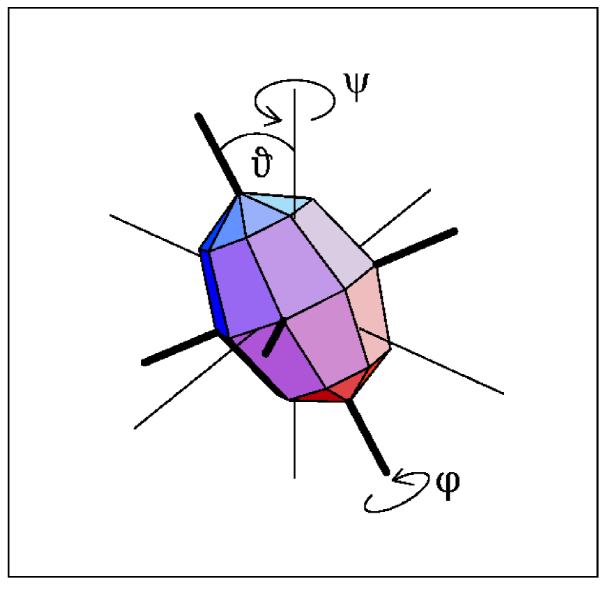
FIG. 1.: The Euler angles specifying the orientation of the triaxial density distribution in the laboratory frame. A polyeder shape is shown, which makes the geometry better visible. The principal axes 1, 2, 3 are fat and the laboratory axes x, y, z are thin.

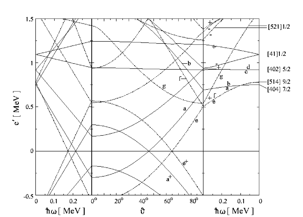
FIG. 2.: Quasi proton energies for $\varepsilon=0.258,~{}\varepsilon_{4}=0.034,~{}\Delta=0.75MeV$. The chemical potential $\lambda$ is adjusted to have $<Z>=72$ at $\omega=0$. Full lines: positive parity, dashed-dotted lines: negative parity. For $\vartheta=90^{o}$ the signature is indicated by $\pm$ standing for $\alpha=\pm 1/2$.

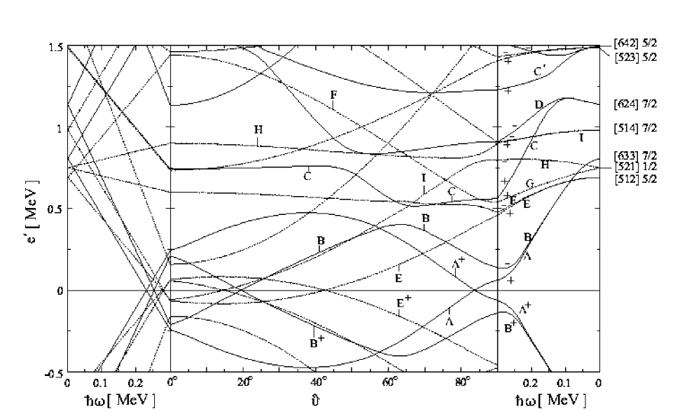
FIG. 3.: Quasi neutron energies for $\varepsilon=0.258,~{}\varepsilon_{4}=0.034,~{}\Delta=0.69MeV$. The chemical potential $\lambda$ is adjusted to have $<N>=102$ at $\omega=0$. Full lines: positive parity, dashed-dotted lines: negative parity. For $\vartheta=90^{o}$ the signature is indicated by $\pm$ standing for $\alpha=\pm 1/2$.

FIG. 4.: Routhians of the configuration [0] for different values of the pair gaps (upper panel) and of the chemical potential $\lambda$ (lower panel). The quantity $E^{\prime}+\lambda_{p}Z+\lambda_{n}N$ is displayed. The pairs of numbers give $(\Delta_{p},\Delta_{n})$ in $MeV$. The values $\lambda_{p}=43.95~{}MeV$ and $\lambda_{n}=49.0~{}MeV$, corresponding to $<Z>=72$ and $<N>=102$ for $\omega=0$, are used in the upper panel. In the lower panel $\lambda_{p}=43.95~{}MeV$ and $\lambda_{n}$ is explicitly indicated in $MeV$. The arrows show at which $\omega$ the condition $<N>=102$ is satisfied.

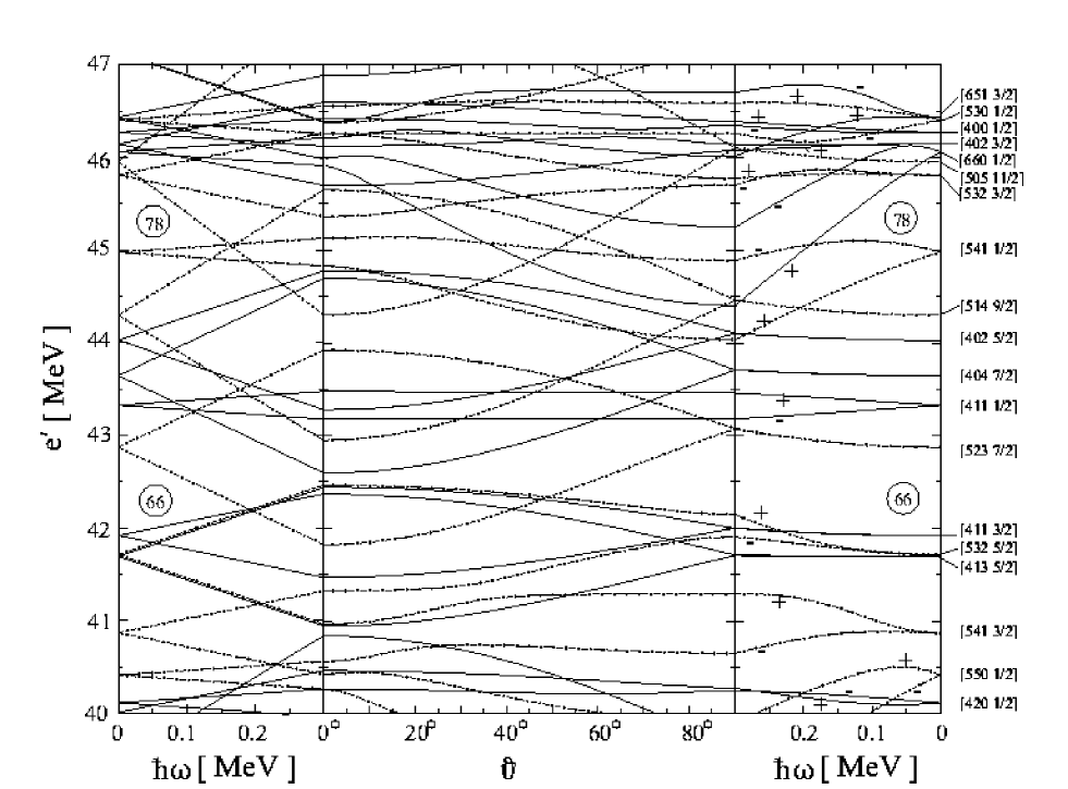
FIG. 5.: Single proton energies at intermediate frequency for $\varepsilon=0.24,~{}\varepsilon_{4}=0$. Full lines: positive parity, dashed-dotted lines: negative parity. For $\vartheta=90^{o}$ the signature is indicated by $\pm$ standing for $\alpha=\pm 1/2$. On the right hand side the Nilsson labels are given, which are relevant for $\omega=0$.

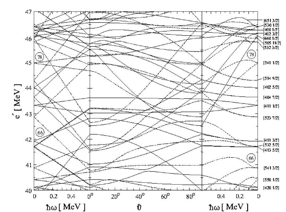
FIG. 6.: Single proton energies at high frequency for $\varepsilon=0.24,~{}\varepsilon_{4}=0$. Full lines: positive parity, dashed-dotted lines: negative parity.

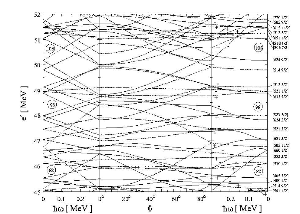
FIG. 7.: Single neutron energies at intermediate frequency for $\varepsilon=0.24,~{}\varepsilon_{4}=0$. Full lines: positive parity, dashed-dotted lines: negative parity. For $\vartheta=90^{o}$ the signature is indicated by $\pm$ standing for $\alpha=\pm 1/2$.

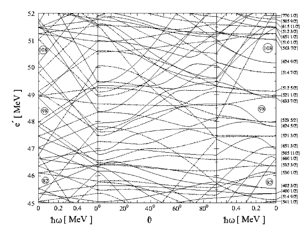
FIG. 8.: Single neutron energies at high frequency for $\varepsilon=0.24,~{}\varepsilon_{4}=0$. Full lines: positive parity, dashed-dotted: lines negative parity.

FIG. 9.: Angular momentum components of different quasi neutrons as function of the tilt angle $\vartheta$ at $\omega=0.3~{}MeV$. They are labeled by A, B, … as in fig. 3. The dotted lines show the values $j_{3}=K$ and $j_{1}=j_{1}(\omega=0.3~{}MeV\sin\vartheta,\vartheta=90^{o}$), which are used in the standard CSM treatment of bands with finite $K$. They are labeled by AP, BP, … The parameters of the calculation are same as in fig. 2 and 3.

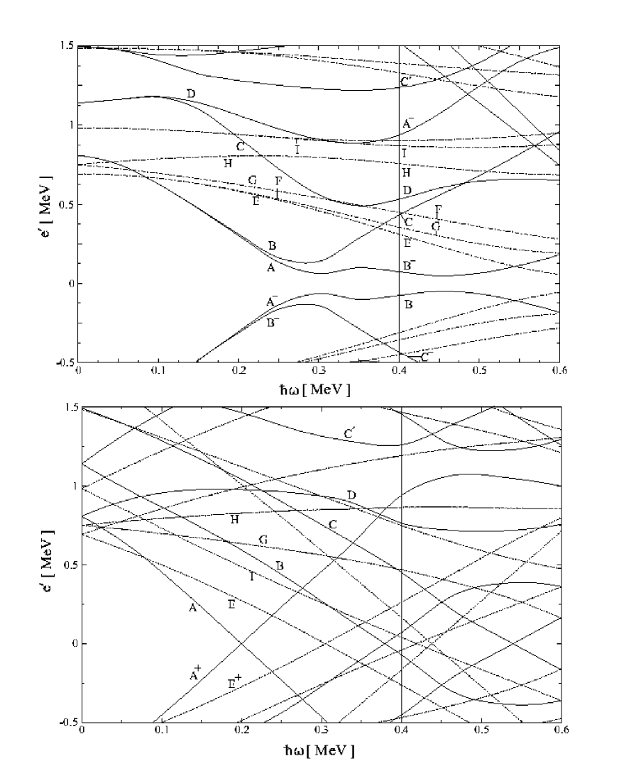
FIG. 10.: Quasi neutron energies for $N\approx 102$ and $\vartheta=90^{o}$ (upper panel) and $\vartheta=45^{o}$ (lower panel). The parameters are $\varepsilon=0.258,~{}\varepsilon_{4}=0.034,~{}\Delta=0.69MeV$. The chemical potential $\lambda$ is adjusted to $<N>=102$ at $\omega=0$ .

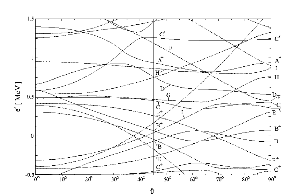
FIG. 11.: Quasi neutron energies for $\varepsilon=0.258,~{}\varepsilon_{4}=0.034,~{}\Delta=0.69MeV$ and $\omega=0.4~{}MeV$. The chemical potential $\lambda$ is adjusted to have $<N>=102$ at $\omega=0$. Full lines: positive parity, dashed-dotted lines: negative parity.

FIG. 12.: Total Routhian as function of the tilt angle for the one quasi neutron configurations in ${}^{175}_{72}$Hf₁₀₃.

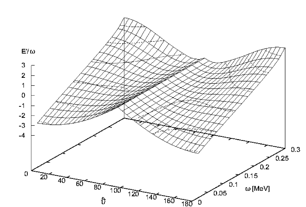
FIG. 13.: Total Routhian $E^{\prime}(\omega,\vartheta)/\omega$ as function of the tilt angle for the one quasi neutron configuration [E] in ${}^{175}_{72}$Hf₁₀₃. The gridlines correspond to the steps $\Delta\vartheta=5^{o}$ and $\Delta\omega=0.02~{}MeV$, starting with $\omega=0.02~{}MeV$. A constant is added such that $E^{\prime}(\omega,\vartheta=90^{o})/\omega=0$.

FIG. 14.: Equilibrium tilt angle $\vartheta_{o}$ as function of the rotational frequency $\omega$ for the one quasi neutron configurations [A] and [E]. The full lines display the TAC result. The dashed lines show the strong coupling estimate, where the moment of inertia ${\cal J}=35~{}MeV^{-1}$ is used, which is the value of $J/\omega$ for the configuration [E].

FIG. 15.: Total Routhians as function of the tilt angle for the lowest positive parity quasi neutron configurations in ${}^{174}_{72}$Hf₁₀₂.

FIG. 16.: Total Routhians of the lowest one quasi neutron configurations in ${}^{175}_{72}$Hf₁₀₃.
The following legend applies to all figures of this type and contains more information than needed for this figure.
The line convention for the parity and signature $(\pi,~{}\alpha)$ is as follows.
Odd $A$: full (+, 1/2), dotted (+, -1/2), dashed dotted (-, 1/2), and dashed (-, -1/2).
Even $A$: full (+, 0), dotted (+, 1), dashed dotted (-, 0), and dashed (-, 1).
Upper panel: Experimental Routhians from the data in [68, 66]. If the bands do not show signature splitting the Routhians are calculated by means of eqs. (70-71) if there is a signature splitting eqs. (70-71) are used. The configuration is given as [X]$K^{\pi}$ where X stands for the letter code explained in the text and $K^{\pi}$ gives the parity $\pi$ and the $K$ value of the band head.
Lower panel: Results of the TAC calculations. For TAC solutions $(\vartheta_{o}\leq 80^{o})$ the two lines representing the signatures are on top of each other. If they are separated the solution is of PAC type $(\vartheta_{o}>80^{o})$. The last TAC point and the first PAC point are connected by a straight line. The grid is $\Delta\omega=0.05~{}MeV$. The band head is only determined with the accuracy of $\Delta\omega$. For several bands the frequency of the first transition ($J(\omega)=K+1$) is indicated by a fat dot.
A rigid rotor reference with ${\cal J}=50~{}MeV^{-1}$ is subtracted from all Routhians.

FIG. 17.: Total Routhians of the lowest one quasi proton configurations in in ${}^{175}_{73}$Ta₁₀₂.
Upper panel: Experimental Routhians from the data in [68, 71]. Lower panel: TAC calculations. Cf. caption of fig. 16.

FIG. 18.: Total Routhians at $\omega=0.2~{}MeV$ as functions of the tilt angle for the lowest configurations in ${}^{174}_{71}$Lu₁₀₃.

FIG. 19.: Total Routhians of the lowest one quasi proton one quasi neutron configurations in ${}^{174}_{71}$Lu₁₀₃.
Upper panel: Experimental Routhians from the data in [73]. Lower panel: TAC calculations. Cf. caption of fig. 16.

FIG. 20.: Branching ratios of the one quasi proton one quasi neutron configuration [aF]${}_{1^{-}}$ in ${}^{174}_{71}$Lu₁₀₃.
Experimental values from [73]. Full line: TAC calculations.

FIG. 21.: Total Routhians as functions of the tilt angle for negative parity lowest two quasi neutron configurations in ${}^{174}_{72}$Hf₁₀₂.

FIG. 22.: Total Routhians of the lowest negative parity two quasi neutron configurations in ${}^{174}_{72}$Hf₁₀₄. Upper panel: Experimental Routhians from the data in [66]. Lower panel: TAC calculations. Cf. caption of fig. 16.

FIG. 23.: Total Routhians of the two quasi neutron configurations containing the pseudo spin singlet quasi neutrons G and H in ${}^{174}_{72}$Hf₁₀₄. Upper panel: Experimental Routhians from the data in [66]. Lower panel: TAC calculations. Cf. caption of fig. 16.

FIG. 24.: Total Routhians of the lowest quasi neutron configurations in ${}^{174}_{72}$Hf₁₀₂ built on the $K^{\pi}=8^{-}$ two quasi proton excitation.
Upper panel: Experimental Routhians from the data in [66]. Lower panel: TAC calculations. The labels $\Delta$ and 0 denote $\Delta_{n}=0.69~{}MeV$ and 0, respectively. Cf. caption of fig. 16.

FIG. 25.: Total Routhians of the lowest quasi neutron configurations in ${}^{175}_{72}$Hf₁₀₃ built on the $K^{\pi}=8^{-}$ two quasi proton excitation.
Upper panel: Experimental Routhians from the data in [66]. Lower panel: TAC calculations. The labels $\Delta$ and 0 denote $\Delta_{n}=0.69~{}MeV$ and 0, respectively. Cf. caption of fig. 16.

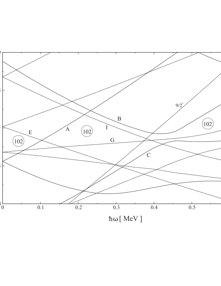
FIG. 26.: Single neutron energies for $\vartheta=45^{o},~{}\varepsilon=0.258,~{}\varepsilon_{4}=0.034$.

FIG. 27.: Total Routhians of the lowest neutron configurations in ${}^{174}_{72}$Hf₁₀₂ built on the $K^{\pi}=8^{-}$ two quasi proton excitation. The TAC calculations assume zero neutron pairing. Cf. caption of fig. 16.

FIG. 28.: Branching ratios of the configuration [aeAE]${}_{14^{+}}$ and [aeAEGI]${}_{18^{+}}$ in ${}^{174}_{72}$Hf₁₀₂.
Experimental values from [66]. Full lines: TAC calculations with neutron pairing dashed lines with zero neutron pairing.

$\gamma$	$-270^{o}$		$-180^{o}$		$-120^{o}$		$-60^{o}$		$0^{o}$		$60^{o}$		$120^{o}$
shape	p	t	o	t	p	t	o	t	p	t	o	t	p
1-axis	s	i	l	l	l∗	l	l	i	s	s	s∗	s	s
3-axis	s	s	s∗	s	s	i	l	l	l∗	l	l	i	s

TABLE I.: Association of the principal axes of the triaxial potential with the axes 1 and 3. The shapes are labeled by p (prolate), o (oblate), and t (triaxial). The axes are labeled by l (long), i (intermediate), and s (short). The star indicates a symmetry axis.

REFERENCES

- [1] S. Frauendorf, Nucl. Phys. A557, 259c (1993)
- [2] A. Brockstedt, J. Lytkens-Lindén, M. Bergström, L. P. Eckström, H. Ryde, J. C. Barcelar, J. D. Garrett, G. B. Hagemann, B. Herskind, F. R. May, P. O. Tjøm, S. Frauendorf, Nuclear Physics A571 (1994) 337
- [3] J.R.B.Oliviera, S.Frauendorf, M.A.Deleplanque, R.M.Diamond, F.S.Stephens, C.W.Beausang, J.E.Draper, C.Duyar, E.Rubel, J.A.Becker, E.A.Henry, N.Roy, Physical Review C 47 (1993) R926
- [4] C. J. Pearson, P. M. Walker, C. S. Purry, G. D. Dracoulis, S. Bayer, A. P. Byrne, T. Kibedy, F. G. Kondev, T. Shizuma, R. A. Bark, G. Sletten, and S. Frauendorf, Phys. Rev. Lett. 79 (1997) 605
- [5] Reviol, W., Riedinger, L.L., Wang, X.Z., Zhang, J.-y., Jensen, H.J., Hagemann, G.B., Bark, R.A., Tjom, P.O., Leoni, S., Lonnroth, T., Schnack-Petersen, H., Shizuma, T., Wrzesinski, J., and Semmes, P., 1999, Phys. Rev. C 59, 1351 (1999)
- [6] F. Dönau, S. Frauendorf, O. Vogel, A. Gelberg, and P. von Brentano, Nucl. Phys. A 584 (1994) 241
- [7] T. Horibata and N. Onishi, Phys. Lett. 325 (1994) 283 and Nucl. Phys. A596 (1994) 251
- [8] T. Kutsarova, R. M. Lieder, H. Schnare, G. Hebbinghaus, D. Balabanski, W. Gast, A. Krämer-Flecken, M. A. Bentley, P. Fallon, D. Howe, A. R. Mokhtar, J. F. Sharpey-Schafer, P. Walker, P. Chowdhury, B. Fabricius, G. Sletten, S. Frauendorf, and P. Walker, Nucl. Phys. A 587 ( 1995) 111
- [9] S. Frauendorf, K. Neergård, J. A. Sheikh, and P. M. Walker, Phys. Rev. C, in print
- [10] V. Dimitrov, F. Dönau, and S. Frauendorf, e-print nucl-th/0002043, Phys. Rev. C, submitted
- [11] G. Baldsiefen, H. Hübel, W. Korten, D. Mehta, N. Nenoff, B. V. Thirmuala Rao, P. Willsau, H. Grawe, J. Heese, H. Kluge, K. H. Maier, R. Schubart, S. Frauendorf, H. J. Maier, Nucl. Phys. A 574 (1994) 521
- [12] G. Baldsiefen,P. Maagh, H. Hübel, W. Korten, S. Chmel, M. Neffgen, W. Pohler, H. Grawe, K. H. Maier, K. Spohr, R. Schubart, S. Frauendorf, H. J. Maier, Nucl. Phys. A 592 (1995) 365
- [13] M. Neffgen, G. Baldsiefen, S. Frauendorf, H. Grawe, J. Heese, H. Hübel, H. Kluge, A. Korichi, W. Korten, H. J. Maier, K. H. Maier, J. Meng, D. Mehta, N. Nenoff, M. Piiparinen, M. Schönhofer, R. Schubart, U. J. van Severen, N. Singh, G. Sletten, B. V. Thirumala Rao, P. Wilssau, Nucl. Phys. A 595 (1995) 499
- [14] R. M. Clark, S. J. Aszatalos, G. Baldsiefen, J. A. Becker, L. Berstein, M. A. Deleplanque, R. M. Diamond, P. Fallon, I. M. Hibbert, H. Hübel, R. Krücken, I. Y. Lee, A. O. Macchiavelli, R. M. MacLeod, G. Schmid, F. S. Stephens, K. Vetter, R. Wadsworth and S, Frauendorf, Phys. Rev. Lett. 78 (1997) 1868
- [15] A. Gadea, G. de Angelis, C. Fahlander, M. De Poli, E. Farnea, Y. Li, D.R. Napoli, Q. Pan, S.M. Lenzi, P. Spolaore, D. Bazzacco, S. Lunardi, C.M. Petrache, P. Pavan, C. Rossi Alvarez, M. Sferrazza, P.G. Bizzeti, A.M. Bizzeti Sona, J. Nyberg, M. Lipoglavsek, J. Persson, J. Cederkäll, D. Seweryniak, A. Johnson, H. Grawe, F. Soramel, M. Ogawa, A. Makishima, R. Schubart and S. Frauendorf, Phys. Rev. C 55 (1997) R1
- [16] Jenkins, D.G., Hibbert, I.M., Parry, C.M., Wadsworth, R., Fossan, D.B., Lane, G.J., Sears, J.M., Smith, J.F., Clark, R.M., Krücken, R., Lee, I.Y., Macchiavelli, A.O., Janzen, V.P., Cameron, J., and Frauendorf, S., Phys. Lett. B 428, 23 (1998)
- [17] D.G. Jenkins, R. Wadsworth , J. Cameron, R.M. Clark,M D.B. Fossan, I.M. Hibbert, V.P. Janzen, R. Krücken, G.J. Lane, M I.Y. Lee, A.O. Macchiavelli, C.M. Parry, J.M Sears, J.F. Smith,M and S. Frauendorf, Phys. Rev. C 58, (1998) 2703
- [18] Clark, R.M., Asztalos, S.J., Busse, B., Chiara, C.J., Cromaz, M., Deleplanque, M.A., Diamond, R.M., Fallon, P., Fossan, D.B., Jenkins, D.G., Juutinen, S., Kelsall, N., Krücken, R., Lane, G.J., Lee, I.Y., Macchiavelli, A.O., MacLeod, R.W., Schmid, G., Sears, J.M., Smith, J.F., Stephens, F.S., Vetter, K., Wadsworth, R., and Frauendorf, S., Phys. Rev. Lett. 82, 3220 (1999)
- [19] Jenkins, D.G., Wadsworth, R., Cameron, J., Clark, R.M., Fossan, D.B., Hibbert, I.M., Janzen, V.P., Krücken, R., Lane, G.J., Lee, I.Y., Macchiavelli, A.O., Parry, C.M., Sears, J.M., Smith, J.F., and Frauendorf, S., Phys. Rev. Lett., 83 (1999) 500
- [20] Chiara, C. J., Asztalos, S. J., Busse, B., Clark, R. M., Cromaz, M., Deleplanque, M. A., Diamond, R. M., Fallon, P., Fossan, D. B., Jenkins, D. G., Juutinen, S., Kelsall, N., Krücken, R., Lane, G. J., I.Y.Lee, A.O.Macchiavelli, R.W.MacLeod, G.Schmid, J.M.Sears,J. F.Smith, F.S.Stephens, K.Vetter, R.Wadsworth, and S.Frauendorf, Phys. Rev. C 61 (2000) 034318
- [21] Kelsall, N.S., Wadsworth, R., Asztalos, S.J., Busse, B., Chiara, C.J., Clark, R.M., Deleplanque, M.A., Diamond, R.M., Fallon, P., Fossan, D.B., Jenkins, D.G., Juutinen, S., Krücken, R., Lane, G.J., Lee, I.Y., Macchiavelli, A.O., Parry, C.M., Schmid, R.W., Sears, J. .M., Stephens, F.S., Smith, J.F., and Vetter, K., Phys. Rev.C 61 (2000) 011301 (R)
- [22] F. Brandolini, M. Ionescu-Bujor, N. H. Medina, R.V. Ribas, D. Bazzacco, M. De Poli, P. Pavan, C. Rossi-Alvarez, G. De Angelis, D. De Acunã, S. Lunardi, D.R. Napoli and S. Frauendorf, B 388 (1996) 468
- [23] Novak, J.R., Beausang, C.W., Amzal, N., Casten, R.F., Cata Danil, G., Cocks, J.F.C., Cooper, J.R., Greenlees, P.T., Hannachi, F., Helariutta, K., Jones, P., Julin, R.,M Juutinen, S., Kankaanpää, H., Kettunen, H., Krücken, R., Kuusiniemi, P., Leino, M., Liu, B., Muikku, M., Savelius, A., Socci, T., Thomas, J.T., Zamfir, N.V., Zhang, J.-y., and Frauendorf, S., Phys. Rev. C 59 (1999) R2989
- [24] Schnare, H., Schwengner, R., Frauendorf, S., Dönau, F.,M Käubler, L., Prade, H., Jungclaus, A., Lieb, K.P.,M Lingk, C., Skoda, S., Eberth, J., de Angelis, G., Gadea, A.,M Farnea, E., Napoli, D.R., Ur, C.A., and LoBianco, G., Phys. Rev. Lett. 82 (1999) 4408
- [25] S. Frauendorf. Z. Phys. A385 (1997), 163
- [26] S. Frauendorf, Rev. Mod. Phys., subm.
- [27] D. J. Thouless and J. G. Valatin, Nucl. Phys. 31 (1962) 211
- [28] M. G. Vassanji and M. Harvey, Nucl. Phys. A344 (1980) 61
- [29] Marshalek, E. R. 1979, Nucl. Phys., A331, 429
- [30] Kerman, A. K, Onishi, N., 1981, Nucl. Phys. A361, 179
- [31] Frisk, H., Bengtsson, R., 1987, Phys. Lett. 196B, 14
- [32] R. Bengtsson, H. Frisk and C.-S. Wu, Proc. of the XXII Zakopane School on Physics, Zakopane, Poland, 1987; Lund Institue of Technology Report Lund-Mph- 87/10
- [33] R. Bengtsson, Nucl. Phys. A 557 (1993) 277c
- [34] A. L. Goodman, Phys. Rev. C 45 (1992) 1649
- [35] F. Cuypers, Nucl. Phys. A468 (1987) 237
- [36] W. Nazarewicz and Z. Szymański, Phys. Rev. C45 (1992) 2771
- [37] E. R. Marshalek, Phys. Rev. C35 (1987) 1900 and C36 (1987) 2538
- [38] E. R. Marshalek, Symp. on Contemporary Physics, Drexel 1991, ed. by Vallieres, M. and Feng, D. H. (World Scientific, Singapore) p.191
- [39] E. R. Marshalek, Nucl. Phys. A557 (1993) 291c
- [40] A. L. Goodman, Nucl. Phys. A542 (1992) 237
- [41] F. A. Dodaro and A. L. Goodman, Phys. Rev. C49 (1994) 1482.
- [42] F. A. Dodaro and A. L. Goodman, Nucl. Phys. A 596 (1996) 91.
- [43] Alhassid, Y, Bush, B., 1991, Nucl. Phys. A531, 39
- [44] W. D. Heiss and R. G. Nazmitdinov, Phys. Lett. B 397 (1997) 1
- [45] T. Horibata, M. Oi and N. Onishi, Phys. Lett. 355 (1995) 433
- [46] F. Dönau, Jing-je Zhang and L. L. Riedinger, Phys. Lett. B 450 , 313 (1999)
- [47] R. Bengtsson, and S. Frauendorf, Nucl. Phys. A314 (1979) 27
- [48] D. Almehet, S. Frauendorf and F. Dönau, Phys. Rev. C, to be published
- [49] P. Ring and P. Schuck, The Nuclear Many Body Problem, Springer (1980)
- [50] S. G. Nilsson and I. Ragnarsson, Shapes and Shells in Nuclear Structure, Cambridge University Press (1995)
- [51] V. M. Strutinsky, Nucl. Phys. A95 (1967) 420
- [52] S. G. Nilsson, C. F. Tsang, A. Sobiczewski, Z. Szymanski, S. Wzcech, C. Gustafson, I. L. Lamm, P. Möller, and B. Nilsson, Nucl. Phys. A131 (1969) 1
- [53] A. Bohr and B. Mottelson, Nuclear Structure II, Benjamin (1975)
- [54] S. Frauendorf, J. Meng, J. Reif, Proc. Conf. on Physic from Large - Ray Detector Arrays, Berkeley 1994, LBL - 35687, Conf - 940888, UC - 413, p. 52
- [55] S. Frauendorf, Proc. of Workshop on Gammasphere Physics, December 1-2, 1995, Berkeley USA, World Scientific Pub., (1996), p. 272
- [56] S. Frauendorf, Z. Phys. A 358 (1997) 163
- [57] T. Bengtsson and I. Ragnarsson, Nucl. Phys. A436 (1985) 14
- [58] S. Chmel, S. Frauendorf, H. Hübel, in preparation
- [59] Y. R. Shimizu, J. D. Garrett, R. A. Broglia, M. Gallardo and E. Viggezzi, Rev. Mod. Phys. 61 (1989) 131
- [60] S. Frauendorf, Phys. Scripta, 24, 349 (1981)
- [61] A. Bohr, I. Hamamoto and Ben R. Mottelson, Physica Scripta 26 (1982) 267
- [62] S. Frauendorf and J. Meng, Z. Phys. A356 (1996) 26
- [63] F. Dönau, S. Frauendorf, Proceedings of the Conference on High Angular Momentum Properties of Nuclei, Oak Ridge Tennessee USA 1982 ed. N. R. Johnson in Nuclear Science Research Conferences Series V. 4 Harwood NY 1983
- [64] Dönau, F., Nucl. Phys. A 471 (1987) 469
- [65] Nuclea Data Sheets
- [66] N. Gjørup, P. M. Walker, G. Sletten, M. A. Bentley, B. Fabricius, and J. F. Sharpey-Schafer, Nucl. Phys. A582 (1995) 369 and N. Gjørup, Thesis, University of Copenhagen, 1994
- [67] H. J. Jensen, G.B. Hagemann, P. O. Tjom, S. Frauendorf, A. Atac, M. Bergström, A. Bracco, A. Brockstedt, H. Carlsson, P. Eckström, J. M. Espino, B. Herskind, F. Ingbretsen, J. Jongman, S. Leoni, R.M. Lieder, T. Lönnroth, A. Maj, B. Million, A. Nordlund, J. Nyberg, M. Piiparinen, H. Ryde, M. Sugawara, A. Virtanen, Z. Physik A 340 (1991) 351 and earlier work cited therein
- [68] Nuclear Data Sheets
- [69] P. M. Walker, G. D. Dracoulis, A. P. Byrne, B. Fabricius, T. Kibedi, A. Stuchbery, Phys. Rev. Lett. 67 (1991) 433
- [70] P.M. Walker, K. C. Yeung, G. D. Dracoulis, P. H. Reagan, G. J. Lane, P. M. Davidson, A. Stuchbery, Phys. Lett. B309 (1993) 17
- [71] F. G. Kondev, G. D. Dracoulis, A. P. Byrne, M. Dasgupta, T. Kibedi, and G. J. Lane, Nucl. Phys. A 601 (1996) 195
- [72] G. D. Dracoulis, S. M. Mullins, A. P. Byrne, F. G. Kondev, T. Kibedi, S. Bayer, G. J. Lane, T. R. McGoram and P. M. Davidson, Phys. Rev. C 58 (1998) 1444
- [73] J. Kern, A. Bruder, J. Cl. Dousse, M. Gasser, V. A. Ionescu, a. Lanners, B. Perny, B. Pillar, Ch. Rhême and B. Schaller, Phys. Lett. B 146 (1984) 183
- [74] K. Neergård, P. Vogel, Nucl. Phys. A145 (1970) 33
- [75] S. Frauendorf and Jie Meng, Nucl. Phys. A617 (1997) 131
- [76] V. Dimitrov, S. Frauendorf, and F. Dönau, e-print nucl-th/0001039, Phys. Rev. Lett , in print