Focusing of a Parallel Beam to Form a Point
in the Particle Deflection Plane

Double Beta Decay: Theory, Experiment, and Implications

1 Introduction

Double beta decay is a rare spontaneous nuclear transition in which the nuclear charge changes by two units while the mass number remains the same. It has been long recognized as a powerful tool to study lepton number conservation in general, and neutrino properties in particular. Since the lifetimes of double beta decays are so long, the experiments on double beta decay are very challenging and have led to the development of many generally valuable techniques to achieve extremely low backgrounds.

For the $\beta\beta~{}$decay to proceed, the initial nucleus must be less bound than the final one, but more bound than the intermediate nucleus. These conditions are realized in nature for a number of even-even nuclei (and never for nuclei with an odd number of protons or neutrons). Since the lifetime of the $\beta\beta~{}$decay is always much longer that the age of the Universe, both the initial and final nuclei exist in nature (some of the actinides being the only exceptions). In many of the “candidates” the transition of two neutrons into two protons is energetically possible, with the largest $Q$ value just above 4 MeV. In a few cases the opposite transition, which decreases the nuclear charge, is also possible, but the $Q$ values are typically smaller.

The nuclear $\beta\beta~{}$transition can proceed in several ways. One of them, the $2\nu$ decay

$$(Z,A)\rightarrow(Z+2,A)+e_{1}^{-}+e_{2}^{-}+\bar{\nu}_{e_{1}}+\bar{\nu}_{e_{2}}$$ (1)

conserves the lepton number, while the other one, the $0\nu$ decay

$$(Z,A)\rightarrow(Z+2,A)+e_{1}^{-}+e_{2}^{-}$$ (2)

violates lepton number conservation and is therefore forbidden in the standard electroweak theory. The prospect of discovering this neutrinoless double beta decay mode is the driving force of most of the interest in this field. It is the possible window into physics “beyond the Standard Model”.

Double beta decay has been and continues to be a popular topic since first discussed by Maria Goeppert-Meyer in nineteen thirties. There have been numerous earlier reviews, beginning with the “classics” by Primakoff and Rosen Prim , Haxton and Stephenson HS and Doi, Kotani and Takasugi DKT , to the more recent ones, often devoted to particular aspects of the $\beta\beta~{}$decay MV94 ; TZ95 ; SC98 ; SPF98 ; Mo99 ; Kla99 ; Ver99 . Many details are also described in the monograph BV92 . The Review of Particle Physics RPP98 regularly summarizes the most recent experimental data.

Double beta decay in all its modes is a second order weak semileptonic process, hence its lifetime, proportional to ($G_{F}\cos\theta_{C}$)^-4, is so very long. (Here $G_{F}=1.166\times 10^{-5}$GeV^-2 is the Fermi coupling constant, and $\theta_{C}$ is the Cabbibo angle.) The neutrinoless decay can be mediated by a variety of virtual particles, in particular by the exchange of light or heavy Majorana neutrinos. The decay amplitude then depends on the masses and coupling constants of these virtual particles. Independent of the actual mechanism of the $0\nu$ $\beta\beta~{}$decay, its observation would imply that neutrinos necessarily have a nonvanishing Majorana mass SW82 . In fact, if the $0\nu$ decay is actually observed, and its rate measured, one can obtain, at least in principle, a lower limit on that mass Kayser91 .

However, so far no $0\nu$ decay has been observed. This means (barring artificial complete cancellation of the amplitudes which we dismiss as unnatural) that the upper limit of the decay rate can be interpreted as an independent limit for each of the possible amplitudes of the decay. In particular, we can obtain the limit on the properties of light and heavy virtual Majorana neutrinos. Below we concentrate on the decays mediated by these particles. (Other possibilities, e.g., the decays mediated by the new particles predicted by supersymmetry, are discussed in Kla99 ; Ver99 .)

The $\beta\beta~{}$decay with the Majoron emission, $0\nu\chi$ mode,

$$(Z,A)\rightarrow(Z+2,A)+e_{1}^{-}+e_{2}^{-}+\chi~{}.$$ (3)

belongs to the category of the lepton number violating decays, even though the lepton number is formally conserved when $\chi$ is assigned the lepton number $-2$. The hypothetical scalar particle $\chi$, which must be in this case light enough to be emitted in the $\beta\beta~{}$decay, is usually associated with spontaneous breaking of the $B-L$ symmetry Chi80 ; GR81 .

Empirically, it is easy to distinguish between the three decay modes listed above, provided the electron energies are measured. The electron sum energy spectra are determined by the phase space of the outgoing leptons and clearly characterize the decay mode, as schematically illustrated in Figure 1. (Geochemical or milking experiments, however, cannot distinguish between the different $\beta\beta~{}$modes as they determine only the total decay rate.)

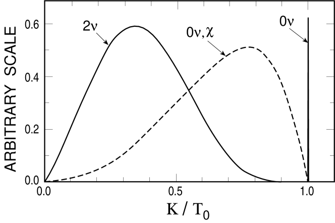
Figure 1: Schematic sum electron spectra of the three $\beta\beta~{}$decay modes. Each is normalized arbitrarily and independently of the others. The abscissa is the ratio $K/T_{0}$ of the sum-electron kinetic energy divided by its maximum value.

There are two distinct groups of theoretical issues associated with the interpretation of the $\beta\beta~{}$decay experiments. The particle physics issues deal with the expression of the decay rate in terms of the fundamental parameters, such as the neutrino masses and mixing angles, coupling constants in the weak interaction Hamiltonian, etc. This group of problems involves also the relation of the $\beta\beta~{}$decay to other processes, such as neutrino oscillations, direct mass measurements, and searches for other lepton number violating processes.

The other, essentially decoupled, set of problems involves the nuclear structure issues associated with the $\beta\beta~{}$decay. The decay rate is expressed in terms of nuclear matrix elements (NME) which have to be evaluated. One would like to know, first of all, their value and its uncertainty. This area of research has attracted lots of attention, and there are many, often conflicting, evaluations available in the literature. Unfortunately, there is no simple way of judging the correctness and accuracy of the evaluations of the nuclear matrix elements for the neutrinoless decay. Comparison to the experimentally known rate of the $2\nu$ $\beta\beta~{}$decay rate is often invoked in that context as a test of the ability of the nuclear model to describe the related phenomena. It is not clear, however, if this is indeed a valid test. For example, if one assumes that the $0\nu$ decay is mediated by the exchange of a heavy particle (whether this exchanged particle is a heavy neutrino or not), the corresponding internucleon potential is of short range, and additional issues involving nucleon structure, irrelevant for the $2\nu$ decay, play an important role. Another, less fundamental but in praxis perhaps more important example deals with the dependence of the NME on the number of single nucleon subshells included in the calculation. For the $2\nu$ decay, where only the Gamow-Teller operator $\sigma\tau$ plays a role, it is clearly sufficient to include just the states within the valence oscillator shell. It is less clear that the same truncation is sufficient for the correct description of the $0\nu$ decay.

The experimental study of the $\beta\beta~{}$decay presents a formidable challenge since the goal is to detect a process with a half-life in excess of $10^{25}$ years (the present best limit for the $0\nu$ decay). The $\beta\beta~{}$decay must be detected in presence of an inevitable background of a similar energy caused by trace radioisotopes with half-lives 15 or more orders of magnitude shorter. Thus, the optimum separation of the signal from background, combined with the requirement of having kilogram quantities of the source isotopes, characterizes the present day experiments.

The past and current experiments are still relatively modest in size, and therefore also in complexity and cost. Given the importance of the search for the neutrinoless decay, ambitious plans, involving much larger amounts of the source nuclei, are considered. Naturally, the larger source mass will be beneficial only if it is accompanied by the corresponding reduction of the background. The future projects will be therefore inevitably much more complex, and will involve larger groups of researchers. With them, the field of $\beta\beta~{}$decay, which competes already with the other experiments described in this book in importance, will also compete in size and cost.

2 Lepton number violation

With the usual assignment of the lepton number, $L(l^{-})=L(\nu)=-L(l^{+})=-L(\bar{\nu})=+1$, $0\nu$ $\beta\beta~{}$decay represents a change in the global lepton number by two units, $\Delta L=2$. In that respect its observation would be related to the attempts to detect $\bar{\nu}_{e}$ from the sun, or of $\nu_{e}$ from nuclear reactors. Both of these latter processes represent a kind of “$\nu\leftrightarrow\bar{\nu}$ oscillations”, and also are possible only for massive Majorana neutrinos.

For light Majorana neutrinos the lepton number conservation is irrelevant and the $0\nu$ decay is hindered only by the helicity mismatch. However, the “antineutrino” born in association with one of the $e^{-}$ in the $0\nu$ decay is not fully righthanded, but has a lefthanded component of amplitude $\sim m_{\nu}/E_{\nu}$. This lefthanded piece can be absorbed by another neutron which is converted into a proton and the second $e^{-}$ is emitted. Similar consideration would govern the above mentioned $\nu\leftrightarrow\bar{\nu}$ oscillations. The word “oscillations” in this context is a misnomer, however, since the process (if it exists) would proceed without an oscillatory behavior KFM99 .

The expected branching ratio for the “wrong” neutrinos at low energies, relevant for the sun or nuclear reactors is LW98

$$R\sim\frac{m_{\nu}^{2}}{2E_{\nu}^{2}}\frac{\sigma^{\bar{\nu}N}}{\sigma^{\nu N}}~{}\sim~{}10^{-14}~{},$$ (4)

where the numerical factor was derived for $m_{\nu}\sim 1$ eV, $E_{\nu}\sim 5$ MeV, and the ratio of cross sections put to unity. Since the $0\nu$ $\beta\beta~{}$decay is presently sensitive to such neutrino masses, one cannot expect a signal for this kind of $\nu\leftrightarrow\bar{\nu}$ oscillations until similar sensitivity is achieved, i.e., not anytime soon, if ever.

However, it is also possible that $\bar{\nu}_{e}$ from the sun are produced in a more complicated, but possibly more efficient way. Let us assume that a transition magnetic moment $\mu_{e,l}$ connects the lefthanded $\nu_{e,L}$ with a righthanded $\bar{\nu}_{l,R}$ of a different flavor, which can subsequently oscillate (by the vacuum or matter enhanced oscillations) into the righthanded and thus observable $\bar{\nu}_{e,R}$, i.e., when neutrinos propagate in a transverse solar magnetic field $B_{\perp}$ one or both of the sequences $\nu_{e,L}\rightarrow\bar{\nu}_{l,R}\rightarrow\bar{\nu}_{e,R}$ or $\nu_{eL}\rightarrow\nu_{l,L}\rightarrow\bar{\nu}_{eR}$ occurs. Such process requires that the magnetic conversion, which is possible only for the massive Majorana neutrinos and which depends on the product $\mu_{e,l}B_{\perp}$, and the flavor oscillation, which depends on $\Delta m^{2}$ and sin${}^{2}2\theta$, are both present. There is no obvious relation between this process and the neutrinoless $\beta\beta~{}$decay, except that both require the existence of the neutrino Majorana mass term. (This brief discussion of the magnetic conversion is highly simplified. In reality, the transition magnetic moments ought to be written in terms of mass eigenstates BV99 .)

Finally, tight experimental limits exist on the total lepton number violating processes which involve both electrons and muons (see RPP98 ), such as the muon conversion

$$\mu^{-}+(Z,A)\rightarrow(Z-2,A)+e^{+}~{},$$ (5)

and the muonium-antimuonium conversion

$$\mu^{+}~{}e^{-}\rightarrow\mu^{-}~{}e^{+}~{}.$$ (6)

The relation of these processes to the $\beta\beta~{}$decay is, however, not well established.

3 Particle physics aspects

In this section we shall consider how the rate of the neutrinoless $\beta\beta~{}$decay is related to the unknown parameters of the neutrino mass matrix and to the phenomenological parameters describing a generalized semileptonic charged current weak interactions $H_{W}$:

$$H_{W}~{}=~{}\frac{G_{F}}{\sqrt{2}}\left[J_{L}^{\alpha}(M_{L\alpha}^{+}+\kappa M_{R\alpha}^{+})~{}+~{}J_{R}^{\alpha}(\eta M_{L\alpha}^{+}+\lambda M_{R\alpha}^{+})\right]~{}+~{}\rm H.c.~{},$$ (7)

where $J_{L(R)}$ and $M_{L(R)}$ are the lepton and quark left(right)-handed current four-vectors, respectively. The dimensionless parameters $\eta,\lambda,$ and $\kappa$ characterize deviations from the standard model. (Since $\kappa$ gives a negligible contribution to double beta decay, we will not consider it from now on.) The coupling parameters $\eta$ and $\lambda$, modified by the neutrino mixing, and denoted then usually as $\langle\eta\rangle$ and $\langle\lambda\rangle$ are unknown (and presumably small).

The lepton sector of the theory contains in general $n$ generations of charged leptons as well as $n$ left- and $n$ right-handed neutrinos. The neutrino mass matrix is the $2n\times 2n$ matrix $M$

$$M=\left(\begin{array}[]{cc}M_{L}&M_{D}^{T}\\ M_{D}&M_{R}\end{array}\right)~{},$$ (8)

where $M_{D}$ is the $n\times n$ lepton number conserving Dirac mass term, and the symmetric $n\times n$ matrices $M_{L}$ and $M_{R}$ are the lepton number violating Majorana mass terms. The matrix $M$ has $2n$ real, but not necessarily positive, eigenvalues. Writing the eigenvalues as $m_{j}\epsilon_{j}$, we can impose the physically reasonable condition that $m_{j}\geq 0$. The sign of the eigenvalues of the mass matrix is contained in the phases $\epsilon_{j}=\pm 1$ which are the intrinsic $CP$ parities of the neutrinos $j$.

Neutrino oscillation phenomena arise because the “mass eigenstates” of $M$ or, more precisely their chiral projections $N_{j}^{L}$ and $N_{j}^{R}$, are not necessarily the familiar weak interaction neutrinos that couple to the known intermediate vector boson $W_{L}$ and to the hypothetical right-handed boson $W_{R}$. The physical “weak eigenstate” or current neutrinos, the $n$ left-handed neutrinos $\nu_{L}$ and the $n$ right-handed ones $\nu_{R}^{{}^{\prime}}$ (the prime has been added in order to stress that they are different particles), are related to the neutrinos of definite mass by the $n\times 2n$ mixing matrices $U$ and $V$

$$\nu_{L}~{}=~{}UN^{L}~{}~{},~{}~{}\nu_{R}^{{}^{\prime}}~{}=~{}VN^{R}~{}.$$ (9)

The mixing matrices $U$ and $V$ obey the normalization and orthogonality conditions

$$\sum_{j=1}^{2n}U_{lj}^{*}U_{l^{\prime}j}~{}=~{}\delta_{ll^{\prime}}~{},~{}\sum_{j=1}^{2n}V_{lj}^{*}V_{l^{\prime}j}~{}=~{}\delta_{ll^{\prime}}~{},~{}\sum_{j=1}^{2n}U_{lj}^{*}V_{l^{\prime}j}~{}=~{}0~{}.$$ (10)

In neutrinoless $\beta\beta~{}$decay the rate depends on the effective parameters which are expressed in terms of the mixing matrices $U$ and $V$:

$$\langle m_{\nu}\rangle~{} = ~{}\sum_{j}{{}^{{}^{\prime}}}\epsilon_{j}m_{j}U_{e,j}^{2}~{},$$

$$\langle\lambda\rangle~{} = ~{}\lambda\sum_{j}{{}^{{}^{\prime}}}\epsilon_{j}U_{e,j}V_{e,j}~{},$$ (11)

$$\langle\eta\rangle~{} = ~{}\eta\sum_{j}{{}^{{}^{\prime}}}\epsilon_{j}U_{e,j}V_{e,j}~{},$$

$$\langle g_{\nu,\chi}\rangle~{} = ~{}\frac{1}{2}\sum_{i,j}{{}^{{}^{\prime}}}(g_{i,j}\epsilon_{i}+g_{j,i}\epsilon_{j})~{}U_{e,i}U_{e,j}~{}.$$

Here the prime indicates that the summation is over only relatively light neutrinos. Also, $\lambda$ and $\eta$ are the dimensionless coupling constants for the right-handed current weak interaction, Eq.(7), and $g_{i,j}$ are the coupling constants of interaction between the Majoron $\chi$ and the Majorana neutrinos $N_{i}$ and $N_{j}$. For the heavy neutrino one obtains

$$\langle m_{\nu}^{-1}\rangle_{H}~{}=~{}\sum_{j}{{}^{{}^{\prime\prime}}}\epsilon_{j}m_{j}^{-1}U_{e,j}^{2}~{},$$ (12)

where the double prime indicates that the summation, involving the inverse neutrino masses $m_{j}^{-1}$, is over only the heavy neutrino mass eigenstates ($m_{j}\geq$1 GeV).

It is now clear that, within the mechanism considered so far, there is no neutrinoless double beta decay if all neutrinos are massless. Not only $\langle m_{\nu}\rangle$ vanishes in such a case but also $\langle\lambda\rangle$ and $\langle\eta\rangle$ vanish due to the orthogonality condition Eq. (10). Moreover, $\langle\lambda\rangle$ and $\langle\eta\rangle$ vanish for the same reason even if some or all neutrinos are massive but light and therefore the summation in Eq.(3) contains all neutrino mass eigenstates. In that case, however, there is a smaller next order contribution from the mass dependence of the neutrino propagator, which for this purpose can be written as

$$\frac{\gamma_{\mu}q^{\mu}}{q^{2}+m_{j}^{2}}~{}\approx~{}\frac{\gamma_{\mu}q^{\mu}}{q^{2}}\left(1-\frac{m_{j}^{2}}{q^{2}}\right)~{}.$$ (13)

The expression for e.g., $\langle\lambda\rangle$ now contains $\sum_{j}{{}^{{}^{\prime}}}\epsilon_{j}U_{e,j}V_{e,j}m_{j}^{2}$ which clearly shows that a nonvanishing neutrino mass is required.

The presence of the phases $\epsilon_{j}$ in the expression for $\langle m_{\nu}\rangle$ means that cancellations are possible. In particular, for every Dirac neutrino there is an exact cancellation, since the Dirac neutrino is equivalent to a pair of Majorana neutrinos with the opposite sign of the phases $\epsilon_{j}$ and degenerate masses.

In the general case the neutrinoless double beta decay rate is a quadratic polynomial in the unknown parameters

$$[T_{1/2}^{0\nu}(0^{+}\rightarrow 0^{+})]^{-1} = C_{1}\frac{\langle m_{\nu}\rangle^{2}}{m_{e}^{2}}+C_{2}\langle\lambda\rangle\frac{\langle m_{\nu}\rangle}{m_{e}}\cos\psi_{1}+C_{3}\langle\eta\rangle\frac{\langle m_{\nu}\rangle}{m_{e}}\cos\psi_{2}$$ (14)

$$+ C_{4}\langle\lambda\rangle^{2}+C_{5}\langle\eta\rangle^{2}+C_{6}\langle\lambda\rangle\langle\eta\rangle\cos(\psi_{1}-\psi_{2})~{}.$$

Here $\psi_{1}$ and $\psi_{2}$ are the phase angles between the generally complex numbers $m_{\nu}$, $\lambda$ and $\eta$. (However, when $CP$ invariance is assumed $\psi_{1,2}$ are either 0 or $\pi$.) The phase space integrals and the nuclear matrix elements are combined in the factors $C_{i}$. Assuming that we can calculate them, Eq. (14) represents an ellipsoid which restricts the allowed range of the unknown parameters $\langle m_{\nu}\rangle$, $\langle\lambda\rangle$ and $\langle\eta\rangle$ for a given value (or limit) of the $0\nu$ double beta decay lifetime.

In order to evaluate the nuclear matrix elements, we must consider the neutrino propagator. Assuming that $\langle m_{\nu}\rangle^{2}$ is the only relevant quantity, one can perform the integration over the four-momentum of the exchanged particle and obtain the “neutrino potential”, which for $m_{\nu}<$ 10 MeV has the form

$$H(r,\Delta E)~{}=~{}\frac{2R}{\pi r}\int_{0}^{\infty}dq\frac{\sin(qr)}{q+\Delta E}~{},$$ (15)

where $\Delta E=\langle E_{N}\rangle-1/2(M_{i}+M_{f})$ is the average excitation energy of the intermediate odd-odd nucleus and the factor $R$ (the nuclear radius) has been added to make the neutrino potential dimensionless.

When the $0\nu$ decay is mediated by the right-handed weak current interaction the evaluation of the decay rate becomes more complicated, since many more terms must be included (see HS ; DKT ; Tomoda ). If the four-momentum of the virtual neutrino is $q_{\mu}\equiv\omega,\vec{q}$, the neutrino propagator contains

$$\omega\gamma_{0}-\vec{q}\cdot\vec{\gamma}+m_{j}~{}.$$

The part of the propagator proportional to $m_{j}$ is responsible for the neutrino potential Eq.(15). The part containing $\vec{q}$ leads to a new potential related to the derivative of $H(r,\Delta E)$, and the part with $\omega$ leads to yet another potential, which is a combination of $H(r,\Delta E)$ and its derivative.

Similarly, there are now also more nuclear matrix elements, which contain in addition the nucleon momenta (i.e., the gradient operators), and depend on the nucleon spins and radii in a more complicated way (e.g., they contain tensor operators). The outgoing electrons are no longer just in the $s_{1/2}$ states, because for some of the operators one of the electrons will be in the $p_{1/2}$ state. The recoil matrix element, which originates from the recoil term in the nuclear vector current is numerically relatively large Tomoda , resulting in more sensitivity to the parameter $\langle\eta\rangle$. The current best limits on $\langle\eta\rangle$ and $\langle\lambda\rangle$ are listed in RPP98 .

4 Experimental techniques and results

It is beyond the scope of this review to describe in detail the experimental techniques developed to meet the challenge of background suppression and signal recognition needed to determine the rate (or an interesting limit) of the $\beta\beta~{}$decay. Thus, only the briefest outline is given, and the most important experimental results are summarized in tables.

Historically, the existence of $\beta\beta~{}$decay was first established using the geochemical method. Here one takes advantage of geologic integration times by searching for daughter products accumulated in ancient minerals that are rich in the parent isotope. (The related radiochemical method is applicable if the daughter isotope is radioactive.) Since the energy information is long lost, the mode of $\beta\beta~{}$decay responsible is not directly determined. Instead, the total decay rate is determined, and thus an upper limit of each mode as well.

Only by measuring the energies of electrons released in the decay in the direct counting experiments can one distinguish directly the mode of decay. The $2\nu$ and $0\nu\chi$ decay modes each result in a rather generic looking electron spectrum (see Fig.1), and the observation of these decays requires either an extremely efficient background suppression or additional information, such as a tracking capability.

The measured half-lives of the $2\nu$ mode are collected in Table 1. Many of them have been measured by several groups; only the results with the smallest claimed errors are shown. (The case of ¹³⁰Te where the two competing results have the same error but exclude each other is the only exception.) Also, the numerous half-life limits have been omitted. The $2\nu$ mode is now well established; no doubt many more and more accurate results will become available soon.

In fact, $\beta\beta~{}$decay is becoming a valuable tool of nuclear spectroscopy. The decay of ¹⁰⁰Mo into the excited $0^{+}$ state at 1130 keV in ¹⁰⁰Ru has been observed Barab ; Ludwig . The technique used, the observation of the subsequent $\gamma$ decay cascade, can be readily applied to other nuclei as well. This development not only expands the scope of the experimental study of the $\beta\beta~{}$decay, but allows more detailed comparison between theory and experiment (for an early attempt, see Austyn ).

Table 1: Recent $\beta\beta_{2\nu}$ results.
(Only positive results are listed. The most accurate published values are given, except for ¹³⁰Te where two conflicting results with the same claimed errors are quoted.)

Isotope	T${}_{1/2}^{2\nu}$ (y)	Reference
48Ca	$(4.3_{-1.1}^{+2.4}\pm 1.4)\times 10^{19}$	Bal96
76Ge	$(1.77\pm 0.01~{}_{-0.11}^{+0.13})\times 10^{21}$	Gun97
82Se	$(8.3\pm 1.0\pm 0.7)\times 10^{19}$	Arn98
96Zr	$(3.9\pm 0.9)\times 10^{19}$ geoch	Kaw93
100Mo	$(6.82^{+0.38}_{-0.53}\pm 0.68)\times 10^{18}$	Desilva97
116Cd	$(3.75\pm 0.35\pm 0.21)\times 10^{19}$	Arn96
128Te	$(7.2\pm 0.4)\times 10^{24}$ geoch	Ber92
130Te	$(2.7\pm 0.1)\times 10^{21}$ geoch	Ber92
	$(7.9\pm 1.0)\times 10^{20}$ geoch	Tak96
150Nd	$(6.75_{-0.42}^{+0.37}\pm 0.68)\times 10^{18}$	Desilva97
238U	$(2.0\pm 0.6)\times 10^{21}$ radioch	Tur91

^geoch geochemical determination; total decay rate.
^radioch radiochemical determination; total decay rate

The 0$\nu$ mode can be approached quite differently from 2$\nu$ and 0$\nu,\chi$ modes because of the distinctive character of the 0$\nu$ electron sum spectrum — a monoenergetic line at the full Q-value (see Fig. 1). Obviously, sharp energy resolution of 0$\nu$ detectors is a big advantage which helps to isolate the line from background. As in the case of the 2$\nu$ decay other features, such as tracking, naturally help as well.

The best reported limits for the neutrinoless $\beta\beta~{}$decay modes are collected in Tables 2 and 3. Again, only the most restrictive limits for the given transition are shown. The longest half-life limit, reported for ⁷⁶Ge by the Heidelberg-Moscow collaboration Baud99 , is based on 24.16 kg yr of exposure and uses pulse shape discrimination to suppress the background (in the relevant energy region the background is a mere ($0.06\pm 0.02$) events/(kg$\cdot$yr$\cdot$keV)). In that experiment 7 events were observed in the $3\sigma$ region around the $0\nu$ decay $Q$ value, while from the background extrapolation one expects 13 events. Using this lack of background events an even more stringent limit (the entry in parenthesis in Table 2) is obtained.

The limit based on the Te lifetime ratio in Table 2 is based on the different $Q$ value dependence of the $0\nu$ and $2\nu$ modes. That this offers a valuable tool has been recognized already in the prophetic early paper by Pontecorvo Pont . Even though the corresponding NME are not exactly equal, they are close enough to allow one to use the geochemical lifetime determination here and in Table 3.

Table 2: Best reported limits on T${}_{1/2}^{0\nu}$ and $\langle m_{\nu}\rangle$.
The experimental result is listed first with its reference. This is followed by the limit on $\langle m_{\nu}\rangle$ followed by the reference to the employed nuclear matrix element (NME). Whenever possible the choice of the authors of the experimental paper regarding the NME is respected. See the text for the discussion of uncertainties associated with the evaluation of NME’s.

Isotope	T${}_{1/2}^{0\nu}$ ($10^{22}$ y) (CL%)	exp. ref.	$\langle m_{\nu}\rangle$ (eV)	NME ref.
48Ca	$>0.95$ (76)	You91	$<18.3$	HS
76Ge	$>1600(5700)^{~{}(see~{}1)}$ (90)	Baud99	$<0.4(0.2)^{~{}(see~{}1)}$	Muto
82Se	$>2.7$ (68)	Ell92	$<5$	HS
100Mo	$>5.2$ (68)	Eji96	$<6.6$	Tomoda
116Cd	$>2.9$ (90)	Geor95	$<4.6$	Muto
$\frac{T_{1/2}(130)}{T_{1/2}(128)}$ ${}^{(see~{}2)}$	$(3.52\pm 0.11)\times 10^{-4}$	Ber92	$<1.1-1.5$	Muto ; Engel
136Xe	$>44$ (90)	Leusch98	$<2.3-2.8$	Engel
150Nd	$>0.12$ (90)	Desilva97	$<4.0$	Muto

¹ the first entry is based on the average background and the entry in parenthesis is based on the apparent lack of background counts in the corresponding energy interval.

² geochemical determination of the lifetime ratio

Table 3: The most restrictive Majoron limits.

Isotope	T${}_{1/2}^{0\nu,\chi}$ (y) and (CL %)	$\langle g_{\nu,\chi}\rangle$	Reference
48Ca	$>7.2\times 10^{20}$ (90)	$<5.3\times 10^{-4}$	Bar89b
76Ge	$>1.66\times 10^{22}$ (90)	$<1.8\times 10^{-4}$,	Beck93
82Se	$>2.4\times 10^{21}$ (68)	$<2.3\times 10^{-4}$	Arn98
100Mo	$>5.4\times 10^{21}$ (68)	$<7.3\times 10^{-5}$	Eji96
116Cd	$>1.2\times 10^{21}$ (90)	$<2.1\times 10^{-4}$	Dan98
128Te	$>7.7\times 10^{24~{}geoch}$ (90)	$<3\times 10^{-5}$	Ber92
136Xe	$>7.2\times 10^{21}$ (90)	$<1.6\times 10^{-4}$	Leusch98
150Nd	$>2.8\times 10^{20}$ (90)	$<1\times 10^{-4}$	Desilva97

^geoch geochemical determination; from total decay rate

5 Nuclear structure aspects

The rate of the $2\nu$ $\beta\beta~{}$decay is simply

$$1/T_{1/2}^{2\nu}=G_{2\nu}(E_{0},Z)|M_{2\nu}|^{2}~{},$$ (16)

while for the neutrinoless decay (assuming that it is mediated by a light Majorana neutrino and that there are no right-handed weak interactions), and for the decay with Majoron emission, it is given by

$$1/T_{1/2}^{0\nu} = G_{0\nu}(E_{0},Z)|M_{0\nu}|^{2}\langle m_{\nu}\rangle^{2}~{},$$ (17)

$$1/T_{1/2}^{0\nu,\chi} = G_{0\nu,\chi}(E_{0},Z)|M_{0\nu,\chi}|^{2}\langle g_{\nu,\chi}\rangle^{2}~{}.$$

Here the phase space functions $G(E_{0},Z)$ are accurately calculable, and the nuclear matrix elements $M$ are the topic of this section. Obviously, the accuracy with which the fundamental particle physics parameters $\langle m_{\nu}\rangle$ and $\langle g_{\nu,\chi}\rangle$ can be determined is limited by our ability to evaluate these nuclear matrix elements.

In that context there are three distinct set of problems:

• $2\nu$ decay: the physics of the Gamow-Teller amplitudes

• $0\nu$ decay with the exchange of light massive Majorana neutrinos: no selection rules on multipoles, role of nucleon correlations, sensitivity to nuclear models.

• $0\nu$ decay with the exchange of heavy neutrinos: physics of the nucleon-nucleon states at short distances.

5.1 Two neutrino decay

Since the energies involved are modest, the allowed approximation should be applicable, and the rate is governed by the double Gamow-Teller matrix element

$$M_{GT}^{2\nu}=\sum_{m}\frac{\langle f||\sigma\tau_{+}||m\rangle\times\langle m||\sigma\tau_{+}||i\rangle}{E_{m}-(M_{i}+M_{f})/2}~{}^{\prime}$$ (18)

where $i,f$ are the ground states in the initial and final nuclei, and $m$ are the intermediate $1^{+}$ (virtual) states in the odd-odd nucleus. The first factor in the numerator above represents the $\beta^{+}$ (or ($n,p$)) amplitude for the final nucleus, while the second one represents the $\beta^{-}$ (or ($p,n$)) amplitude for the initial nucleus. Thus, in order to correctly evaluate the $2\nu$ decay rate, we have to know, at least in principle, all GT amplitudes for both $\beta^{-}$ and $\beta^{+}$ processes, including their signs. The difficulty is that the $2\nu$ matrix element exhausts a very small fraction ($10^{-5}-10^{-7}$) of the double GT sum rule double , and hence it is sensitive to details of nuclear structure.

Various approaches used in the evaluation of the $2\nu$ decay rate have been reviewed recently in Ref. SC98 . The Quasiparticle Random Phase Approximation (QRPA) has been the most popular theoretical tool in the recent past. Its main ingredients, the repulsive particle-hole spin-isospin interaction, and the attractive particle-particle interaction, clearly play a decisive role in the concentration of the $\beta^{-}$ strength in the giant GT resonance, and the relative suppression of the $\beta^{+}$ strength and its concentration at low excitation energies. Together, these two ingredients are able to explain the suppression of the $2\nu$ matrix element when expressed in terms of the corresponding sum rule.

Yet, the QRPA is often criticized. Two “undesirable”, and to some extent unrelated, features are usually quoted. One is the extreme sensitivity of the decay rate to the strength of the particle-particle force (often denoted as $g_{pp}$). This decreases the predictive power of the method. The other one is the fact that for a realistic value of $g_{pp}$ the QRPA solutions are close to their critical value (so called collapse). This indicates a phase transition, i.e., a rearrangement of the nuclear ground state. QRPA is meant to describe small deviations from the unperturbed ground state, and thus is not fully applicable near the point of collapse. Numerous approaches have been made to extend the range of validity of QRPA, see e.g. SC98 . Altogether, QRPA and its various extensions, with their ability to adjust at least one free parameter, are typically able to explain the observed $2\nu$ decay rates.

At the same time, detailed calculations show that the sum over the excited states in Eq.(18) converges quite rapidly EEV94 . In fact, a few low lying states usually exhaust the whole matrix element. Thus, it is not really necessary to describe all GT amplitudes; it is enough to describe correctly the $\beta^{+}$ and $\beta^{-}$ amplitudes of the low-lying states, and include everything else in the overall renormalization (quenching) of the GT strength.

Nuclear shell model methods are presently capable of handling much larger configuration spaces than even a few years ago. Thus, for many nuclei the evaluation of the $2\nu$ rates within the 0$\hbar\omega$ shell model space is feasible. (Heavy nuclei with permanent deformation, like ¹⁵⁰Nd and ²³⁸U remain, however, beyond reach of the shell model techniques.) Using the shell model avoids, naturally, the above difficulties of QRPA. At the same time, the shell model can describe, using the same method and the same residual interaction, a wealth of spectroscopic data, allowing much better tests of its predictive power.

5.2 Neutrinoless decay: light Majorana neutrino

If one assumes that the $0\nu$ decay is caused by the exchange of a virtual light Majorana neutrino between the two nucleons, then several new features arise: a) the exchanged neutrino has a momentum $q\sim 1/r_{nn}\simeq 50-100$ MeV ($r_{nn}$ is the distance between the decaying nucleons). Hence, the dependence on the energy in the intermediate state is weak and the closure approximation is applicable and one does not have to sum explicitly over the nuclear intermediate states. Also, b) since $qR>1$ ($R$ is the nuclear radius), the expansion in multipoles is not convergent, unlike in the $2\nu$ decay. In fact, all possible multipoles contribute by a comparable amount. Finally, c) the neutrino propagator results in a neutrino potential of a relatively long range (see Eq. (15)).

Thus, in order to evaluate the rate of the $0\nu$ decay, we need to evaluate only the matrix element connecting the ground states $0^{+}$ of the initial and final nuclei. Again, we can use the QRPA or the shell model. Both calculations show that the features enumerated above are indeed present. In addition, the QRPA typically shows less extreme dependence on the particle-particle coupling constant $g_{pp}$ than for the $2\nu$ decay, since the contribution of the $1^{+}$ multipole is relatively small. The calculations also suggest that for quantitatively correct results one has to treat the short range nucleon-nucleon repulsion carefully, despite the long range of the neutrino potential.

Does that mean that the calculated matrix elements are insensitive to nuclear structure? An answer to that question has obviously great importance, since unlike the $2\nu$ decay, we cannot directly test whether the calculation is correct or not.

Figure 2: The cumulative contribution, i.e., the summed contribution of all natural parity multipoles up to $I$ of the exchanged $nn$ and $pp$ pair, to the $0\nu$ nuclear matrix element combination $M_{GT}^{0\nu}-M_{F}^{0\nu}$. The full line is for ⁷⁶Ge and the dashed line for ⁴⁸Ca.

For simplicity, let us assume that the $0\nu$ $\beta\beta$ decay is mediated only by the exchange of a light Majorana neutrino. The relevant nuclear matrix element is then the combination $M_{GT}^{0\nu}-M_{F}^{0\nu}$, where the GT and F operators change two neutrons into two protons, and contain the corresponding operator plus the neutrino potential. One can express these matrix elements either in terms of the proton particle - neutron hole multipoles (i.e., the usual beta decay operators) or in terms of the multipole coupling of the exchanged pair, $nn$ and $pp$.

When using the decomposition in the proton particle - neutron hole multipoles, one finds that all possible multipoles (given the one-nucleon states near the Fermi level) contribute, and the contributions have typically equal signs. Hence, there does not seem to be much cancellation.

However, perhaps more physical is the decomposition into the exchanged pair multipoles. There one finds, first of all, that only natural parity multipoles ($\pi=(-1)^{I}$) contribute noticeably. And there is a rather severe cancellation. The biggest contribution comes from the $0^{+}$ multipole, i.e., the pairing part. All other multipoles, related to higher seniority states, contribute with an opposite sign. The final matrix element is then a difference of the pairing and higher multipole (or broken pair $\equiv$ higher seniority) parts, and is considerably smaller than either of them. This is illustrated in Fig. 2 where the cumulative effect is shown, i.e., the quantity $M(I)=\sum_{J}^{I}\left[M_{GT}^{0\nu}(J)-M_{F}^{0\nu}(J)\right]$ is displayed for ⁷⁶Ge (from muto2 ) and ⁴⁸Ca (from ca48sm ). Thus, the final result depends sensitively on both the correct description of the pairing and on the admixtures of higher seniority configurations in the corresponding initial and final nuclei. It appears, moreover, that the final result might depend on the size of the single particle space included. That important question requires further study.

Figure 3: Half-lives (in years) calculated for $\langle m_{\nu}\rangle$ = 1 eV by various representative methods and different authors for the most popular double-beta decay candidate nuclei. Solid lines are QRPA from Muto , dashed lines are QRPA from Engel (recalculated for $g_{A}$ = 1.25 and $\alpha^{\prime}=-390$ MeV fm³), dotted lines are shell model HS , and dot-and-dashed lines are shell model Caurier97 .

Since there is no objective way to judge which calculation is correct, one often uses the spread between the calculated values as a measure of the theoretical uncertainty. This is illustrated in Fig. 3. There, I have chosen two representative QRPA sets of results, the highly truncated “classical” shell model result of Haxton and Stephenson, and the result of more recent shell model calculation which is convergent for the set of single particle states chosen (essentially 0$\hbar\omega$ space).

For the most important case of ⁷⁶Ge the calculated rates differ by a factor of 6-7. Since the effective neutrino mass $\langle m_{\nu}\rangle$ is inversely proportional to the square root of the lifetime, the experimental limit of $1.6\times 10^{25}$ y translates into limits of about 1 eV using the NME of Engel ; Caurier97 , and about 0.4 eV with the NME of HS ; Muto . On the other hand, if one would accept the more stringent limit of $5.7\times 10^{25}$ Baud99 , even the more pessimistic matrix elements restrict $\langle m_{\nu}\rangle<0.5$ eV. Needless to say, a more objective measure of the theoretical uncertainty would be highly desirable.

In Tables 2 and 3 we list the deduced limits on the fundamental parameters, the effective neutrino Majorana mass $\langle m_{\nu}\rangle$, and the Majoron coupling constant $\langle g_{\nu,\chi}\rangle$. The references to the source of the corresponding nuclear matrix elements, used to translate the experimental half-life limit into the listed limits on $\langle m_{\nu}\rangle$ and $\langle g_{\nu,\chi}\rangle$ are also given. When using the tables one has to keep in mind the uncertainties illustrated in Fig. 3.

5.3 Neutrinoless decay: very heavy Majorana neutrino

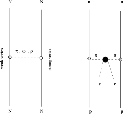
Figure 4: The Feynman graph description of the parity-violating nucleon-nucleon force (left graph) and of the $\beta\beta~{}$decay with the exchange of a heavy neutrino mediated by the pion exchange. The short range lepton number violating amplitude is symbolically described by the filled blob in the right graph.

The neutrinoless $\beta\beta$ decay can be also mediated by the exchange of a heavy neutrino. The decay rate is then inversely proportional to the square of the effective neutrino mass Verg81 . In this context it is particularly interesting to consider the left-right symmetric model proposed by Mohapatra Moh86 . In it, one can find a relation between the mass of the heavy neutrino $M_{N}$ and the mass of the right-handed vector boson $W_{R}$. Thus, the limit on the $\beta\beta$ rate provides, within that specific model, a stringent lower limit on the mass of $W_{R}$.

The process then involves the emission of the heavy $W_{R}^{-}$ by the first neutron and its virtual decay into an electron and the heavy Majorana neutrino, $W_{R}^{-}\rightarrow e^{-}+\nu_{N}$. This is followed by the transition $\nu_{N}\rightarrow e^{-}+W_{R}^{+}$ and the absorption of the $W_{R}^{+}$ on the second neutron, changing it into the second proton. Since all exchanged particles between the two neutrons are very heavy, the corresponding “neutrino potential” is of essentially zero range. Hence, when calculating the nuclear matrix element, one has to take into account carefully the short range nucleon-nucleon repulsion.

As long as we treat the nucleus as an ensemble of nucleons only, the only way to have nonvanishing nuclear matrix elements for the above process is to treat the nucleons as finite size particles. In fact, that is the standard way to approach the problem Verg81 ; the nucleon size is described by a dipole form factor with the cut-off parameter $\Lambda\simeq$ 0.85 GeV. Using such a treatment of the nucleon size, and the half-life limit for the ⁷⁶Ge $0\nu$ decay listed in Table 2, one obtains a very interesting limit on the mass of the vector boson $W_{R}$ Hir96

$$m_{W_{R}}\geq 1.6{\rm~{}TeV}~{}.$$ (19)

However, another way of treating the problem is possible, and already mentioned in Verg81 . Let us recall how the analogous situation is treated in the description of the parity-violating nucleon-nucleon force AH85 . There, instead of the weak (i.e., very short range) interaction of two nucleons, one assumes that a meson ($\pi,\omega,\rho$) is emitted by one nucleon and absorbed by another one. One of the vertices is the parity-violating one, and the other one is the usual parity-conserving strong one. The corresponding range is then just the meson exchange range, easily treated. The situation is schematically depicted in the left-hand panel of Fig. 4. The analogy for $\beta\beta$ decay is shown in the right-hand graph. It involves two pions, and the “elementary” lepton number violating $\beta\beta~{}$decay then involves a transformation of two pions into two electrons. Again, the range is just the pion exchange range. It would be interesting to see if a detailed treatment of this graph would lead to more or less stringent limit on the mass of the $W_{R}$ than the treatment with form factors. The relation to the claim in rho72 that an analogous graph contributing to the lepton number violating muon capture identically vanishes should be further investigated; in fact that claim is probably not valid.

6 Perspectives

As stated earlier, the present best limits on the rate of the $0\nu$ $\beta\beta~{}$decay, or equivalently on the neutrino effective Majorana mass $\langle m_{\nu}\rangle$, were obtained with an exposure of about 20 kg$\cdot$yr. Several experiments (Heidelberg-Moscow ⁷⁶Ge Baud99 , IGEX ⁷⁶Ge IGEX99 , Caltech-Neuchatel TPC ¹³⁶Xe Leusch98 ) are presently at or near that level. The other limits in Tables 2 and 3 were obtained with smaller exposures of $\sim$ 1 kg$\cdot$yr. The detector NEMO-3, with planned source mass of 10 kg, is being built and should be operational soon Nemo99 . In few years of operation it should reach a half-life limit of $\sim 10^{25}$ yr for the $0\nu$ decay of ¹⁰⁰Mo, and perhaps other nuclei as well. However, further improvements with the existing detectors becomes increasingly difficult, since the sensitivity to the $\langle m_{\nu}\rangle$ is proportional to only the 1/4 power of the source mass and exposure time. Thus, much larger sources are clearly needed.

What are the perspectives of a radical improvement in the search for the $0\nu$ $\beta\beta~{}$decay? To achieve that, one would have to build a detector capable of using hundreds of kg or even several tons of the source material. At the same time, the background per unit mass has to be correspondingly improved so that one can benefit from the larger mass. Obviously, such program is very challenging.

The difficulty begins with the problem of acquiring such a large mass of the isotopically separated and radioactively clean material. Here, the principal obstacle is the cost of the isotope separation. (This can be avoided only if the source isotope has large abundance; in practice that is true only for ¹³⁰Te with 34% abundance.)

The second unavoidable difficulty is the background caused by the $2\nu$ decay. One can observe the $0\nu$ decay only if its rate exceeds the fluctuations of the $2\nu$ events at the same energy, i.e., near the decay $Q$ value. The number of $2\nu$ decays in an energy interval $\Delta E$ near $Q$ depends on these quantities like $\sim(\Delta E/Q)^{6}$ provided $\Delta E\ll Q$. (If the energy resolution is folded in, this dependence is somewhat modified.) Thus, good energy resolution, which determines how wide interval $\Delta E$ one must consider, is again crucial in order to reduce the effect of this “ultimate” background.

One of the proposal for such a large $\beta\beta~{}$experiments has been extensively discussed in the literature (see, e.g., Kla99 ). The project, with the acronym GENIUS, would use a large amount of ‘naked’ enriched ⁷⁶Ge, in the form of an array of about 300 detectors, suspended in liquid nitrogen, which provides simultaneously cooling and shielding. It is envisioned that the detector would consist of one ton of enriched ⁷⁶Ge. The anticipated background is 0.04 counts/(keV$\cdot$yr$\cdot$t), i.e., about 1000 times lower than the best existing backgrounds. Such a detector could reach the half-life limit of about $6\times 10^{27}$ yr within one year of operation, thus improving the neutrino mass limit by an order of magnitude.

Another large project, CUORE, Fio98 is a cryogenic set-up consisting of 17 towers, each containing 60 cubic crystals of TeO₂. It would be housed in a single specially constructed dilution refrigerator and would contain about 800 kg of the sensitive material. A prototype system, CUORICINO, consisting of one of the towers, is being developed now.

An experiment with a large amount (100 tons) of natural molybdenum, (abundance of the $\beta\beta~{}$candidate ¹⁰⁰Mo = 9.6%) with good energy and position resolution, is proposed in Ref. Ejiri .

In order to radically suppress the background, the Ba ions, the final products of the ¹³⁶Xe double beta decay, could be identified by laser tagging. That approach, described in Ref. EXO , would allow to use a large Time Projection Chamber with perhaps ton quantities of ¹³⁶Xe, reaching sensitivities to half-lives $\sim 10^{28}$ years.

This, still incomplete list of proposed very large $\beta\beta~{}$decay experiments shows that the field is entering a critical phase. If the new techniques, mentioned above, can be developed in conjuntion with the large source mass, the background caused by radioactivities can be essentially eliminated. However, as stated above, the ultimate background due to the tail of the $2\nu$ decay can be compensated only by a superior energy resolution.

Given the importance of the neutrinoless decay, it is likely that several of these large and costly projects, involving ton$\cdot$years of exposure and a correspondingly reduced background, will be realized in the foreseeable future. Thus, sensitivity to the neutrino Majorana mass $\langle m_{\nu}\rangle$ approaching 0.01 eV may be in sight. Whether the neutrinoless decay will be discovered is unknown, but the reasons to look for it are so compelling, that the search will undoubtedly continue.

7 Implications

The study of $0\nu$ $\beta\beta~{}$decay provides at present an upper limit well below 1 eV for the effective electron neutrino Majorana mass $\langle m_{\nu}\rangle$ even if the most pessimistic nuclear matrix elements are used. What are the consequences of that limit when combined with the manifestations of the neutrino oscillations?

Recall that the atmospheric neutrino anomaly (with its zenith angle dependence) implies the nearly maximum mixing of $\mu$ and $\tau$ neutrinos (or $\mu$ and sterile neutrinos) with $\Delta m^{2}\sim 10^{-3}$ eV² (see chapter 5 of this book). There is, so far, no unique neutrino oscillation solution to the solar neutrino deficit(see chapter 4 of this book). However, all of the acceptable solutions have $\Delta m^{2}<10^{-4}$ eV² and involve electron neutrinos. Both large and small mixing angle solutions are currently compatible with the data. Finally, the third “positive” evidence comes from the LSND experiment (see chapter 7 of this book), and implies relatively small mixing between the electron and muon neutrinos and $\Delta m^{2}\geq 0.1$ eV². A full analysis must contain, in addition, all experimental results which exclude various parts of the possible regions of the quantities $\Delta m^{2}$ and the mixing angles. Taking all these findings together would necessarily imply the existence of a fourth neutrino, which must be “sterile” given the constraint on the invisible width of the $Z$. At the same time, it is well known that oscillation experiments are not able to furnish the overall scale of the neutrino masses.

This absolute neutrino mass scale is essential not only as a matter of principle, but in particular if one wants to ascribe part of the dark matter, namely its “hot” component, to massive neutrinos. Doing that would mean that the sum of the neutrino masses $\sum m_{\nu}$ is one or several eV. Tritium beta decay gives an upper limit of a similar magnitude for any mass eigenstate with a large electron flavor component. Clearly, if light neutrinos are responsible for a nonnegligible part of the dark matter, the oscillation data mean that at least two, and possibly all neutrino masses are nearly degenerate. (Such scenario was discussed for the first time in Ref. David .) The relation of the $0\nu$ $\beta\beta~{}$decay and the oscillation scenarios, in particular the scenarios involving degenerate neutrinos, has been a topic of several recent papers GG98 ; EL99 ; BW99 ; Bil99 .

The consequences are particularly dramatic if one assumes that only three massive Majorana neutrinos exist with nearly degenerate masses $m_{i}\simeq\bar{m}\sim$ $O$(eV). (Hence discarding for this purpose the LSND experimental result, even though there is no evidence against it.) The $\beta\beta~{}$decay constraint can be expressed as GG98

$$\langle m_{\nu}\rangle=|m_{1}c_{2}^{2}c_{3}^{2}e^{i\phi}+m_{2}c_{2}^{2}s_{3}^{2}e^{i\phi^{\prime}}+m_{3}s_{2}^{2}e^{i2\delta}|~{},$$ (20)

where $c_{i},s_{i}$ denote $\cos\theta_{i},\sin\theta_{i}$ in the $3\times 3$ mixing matrix, $\delta$ is the CP violating phase in that matrix, and $\phi,\phi^{\prime}$ are the CP violating phases in the diagonal mass matrix. Clearly, the differences in $m_{i}$ can be neglected in this case. Moreover, the reactor long baseline experiments have established that $\nu_{e}$ do not mix very much with anything else near $\Delta m^{2}\sim 10^{-3}$ eV², which means that the angle $\theta_{2}$ is small. At the same time, the angle $\theta_{1}$ which controls the atmospheric neutrino oscillations is near its maximum value $\sin^{2}2\theta_{1}\simeq 1$. Thus

$$|\cos^{2}\theta_{3}+\sin^{2}\theta_{3}e^{i(\phi^{\prime}-\phi)}|<\langle m_{\nu}\rangle/\bar{m}\ll 1~{}.$$ (21)

Hence also $\theta_{3}$ must be near the maximum mixing, $\sin 2\theta_{3}\simeq 1$, and the CP phases in the above equation (21) are such that the two terms cancel each other.

That would be a very unexpected result. We would have three massive highly degenerate neutrinos with bimaximal mixing. Moreover, the electron neutrino would be ‘quasi-Dirac’ with its two components essentially canceling each other in their contribution to the $0\nu$ $\beta\beta~{}$decay. While such a scenario is rather problematic (see EL99 ), and it does not accommodate the LSND result at all, it illustrates the power of the neutrinoless $\beta\beta~{}$decay in constraining the choice of the neutrino oscillation scenarios.

8 Conclusions

The quest for neutrino mass is at a critical stage at present. The evidence for neutrino mixing is getting stronger and stronger, and the basic parameters describing the neutrino oscillation phenomena are being constrained more and more. At the same time, the oscillation searches cannot give us the scale of the neutrino masses, but only their differences. Among the experiments that are sensitive to the masses themselves, albeit to their different aspects (end point of the ordinary beta decay, observation of the supernova neutrinos, and the neutrinoless double beta decay), only the $0\nu$ decay is able to reach the sub eV region, and in a foreseeable future extend it by a substantial margin.

In this review the present status of the $\beta\beta~{}$decay is described. The unpleasant uncertainty related to the nuclear structure aspect of the problem is estimated to be at the level of a factor of 2-3 for the effective neutrino mass. However, the experimental progress is such that even using the most conservative nuclear matrix elements allows us to push the limit well below the competing techniques. The nuclear structure uncertainty can be reduced by further development of the corresponding nuclear models. At the same time, by reaching comparable experimental limits in several nuclei, the chances of a severe error in the NME will be substantially reduced.

Several projects are under way that will improve the life-time limit substantially, or find the $0\nu$ decay. Already now the search for $\beta\beta~{}$decay gives important constraints on the fundamental properties of neutrinos and their interactions. The role of the $\beta\beta~{}$decay in the whole enterprise descibed in various chapters of this book will be substantially strengthened once these ambitious projects are underway.

Acknowledgment

This work was supported by the US Department of Energy under Grant No. DE-FG03-88ER-40397.

References

- (1) H. Primakoff and S. P. Rosen, Rep. Prog. Phys. 22, 121(1959).
- (2) W. C. Haxton and G. J. Stephenson Jr., Prog. in Part. Nucl. Phys. 12, 409 (1984).
- (3) M. Doi, T. Kotani, and E. Takasugi , Prog. Theor. Phys. Suppl 831 (1985).
- (4) M. Moe and P. Vogel, Ann. Rev. Nucl. Part. Sci. 44, 247 (1994).
- (5) V. I. Tretyak and Yu. Zdesenko, At. Data Nucl. Data Tables 61, 43 (1995).
- (6) J. Suhonen and O. Civitarese, Phys. Rep. 300, 123 (1998).
- (7) F. Šimkovic, G. Pantis, and A. Faessler, Phys. Atom. Nucl. 61, 218 (1998).
- (8) A. Morales, Nucl. Phys. B, Proc. Suppl. 77, 335 (1999).
- (9) H. V. Klapdor-Kleingrothaus, preprint hep-ex/9907040.
- (10) J. D. Vergados, Beyond the Desert 99, Ringberg Castle, June 99; hep-ph/9907316.
- (11) F. Boehm and P. Vogel, Physics of Massive Neutrinos Cambridge University Press, Cambridge, 1992 (Second Edition).
- (12) C. Caso et al, Eur. Phys. J. 3, 1 (1998).
- (13) J. Schechter and J. W. F. Valle, Phys. Rev. D 25, 2951 (1982).
- (14) B. Kayser, Nucl. Phys. B, Proc. Suppl. 19, 177 (1991).
- (15) Y. Chikashige, R. N. Mohapatra, and R. D. Peccei, Phys. Rev. Lett, 45, 1926 (1980).
- (16) G. Gelmini and M. Rondacelli, Phys. Lett. B99, 411 (1981).
- (17) P. Fisher, B. Kayser, and K. D. McFarland, hep-ph/9906244.
- (18) P. Langacker and J. Wang, Phys. Rev. D 58 093004.
- (19) J. Beacom and P. Vogel, Phys. Rev. Lett. 83, 5222 (1999).
- (20) T. Tomoda, Rep. Progr. Part. Phys. 54, 53 (1991).
- (21) A. Balysh et al., Phys. Rev. Lett. 77, 5186 (1996).
- (22) M. Günther et al., Phys. Rev. D 55, 54 (1997).
- (23) R. Arnold et al., Nucl. Phys. A636, 209 (1998).
- (24) A. Kawashima, K. Takahashi, and A. Masuda, Phys. Rev. C 47, 2452 (1993).
- (25) A. De Silva et al., Phys. Rev. C 56, 2451 (1997).
- (26) R. Arnold et al, Z. Phys. C72, 239 (1996).
- (27) T. Bernatowicz et al., Phys. Rev. Lett. 69, 2341 (1992).
- (28) N. Takaoka, Y. Motomura, K. Nagao, Phys. Rev. C 53, 1557 (1996).
- (29) A. L. Turkevich, T. E. Economou, and G. A. Cowan, Phys. Rev. Lett. 67, 3211 (1991).
- (30) A. S. Barabash et al. , Phys. Lett. B345, 408 (1995).
- (31) L. De Braeckeleer et al, preprint, September 1999.
- (32) A. Griffiths and P. Vogel, Phys. Rev. C46, 181 (1992).
- (33) L. Baudis et al., Phys. Rev. Lett. 83, 41 (1999).
- (34) K. E. You et al., Phys. Lett. B265 53 (1991).
- (35) A. Staudt, K. Muto, and H. V. Klapdor-Kleingrothaus, Europ. Lett. 13, 31 (1990).
- (36) S. R. Elliott et al., Phys. Rev. C 46, 1535 (1992).
- (37) H. Ejiri et al., Nucl. Phys. A611, 85 (1996).
- (38) A. Sh. Georgadze et al., Phys. At. Nucl. 58, 1093 (1995).
- (39) J. Engel, P. Vogel, and M. R. Zirnbauer, Phys. Rev. C 37, 731 (1988).
- (40) R. Luescher et al., Phys. Lett. B434, 407 (1998).
- (41) A. S. Barabash , Phys. Lett. B216, 257 (1989).
- (42) M. Beck et al., Phys. Rev. Lett. 70, 2853 (1993).
- (43) F. A. Danevich et al., Nucl. Phys. A643, 317 (1998).
- (44) B. Pontecorvo, Phys. Lett. B26, 630 (1968).
- (45) P. Vogel, M. Ericson, and J. D. Vergados, Phys. Lett. B212, 259 (1988); K. Muto, Phys. Lett. B277, 13 (1992).
- (46) M. Ericson, T. Ericson, and P. Vogel, Phys. Lett. B328, 259 (1994).
- (47) K. Muto, E. Bender, and H. V. Klapdor, Z. Phys. A 334, 187 (1989).
- (48) E. Caurier, A. Poves, and A. P. Zuker, Phys. Lett. B252, 13 (1990).
- (49) E. Caurier, F. Nowacki, A. Poves, and J. Retamosa, Phys. Rev. Lett. 77, 1954 (1996), and E. Caurier, private communication.
- (50) J. D. Vergados, Phys. Rev. C24, 640 (1981).
- (51) R. N. Mohapatra, Phys. Rev. D34, 909 (1986).
- (52) M. Hirsch, H. V. Klapdor-Kleingrothaus, and S. G. Kovalenko, Phys. Lett. B372, 181 (1996).
- (53) E. G. Adelberger and W. C. Haxton, Ann. Rev. Nucl. Part. Sci. 35, 501 (1985).
- (54) M. D. Shuster and M. Rho, Phys. Lett. B42, 54 (1972).
- (55) C. E. Aalseth et al., Phys. Rev. C 59, 2108 (1999).
- (56) X. Sarazin et al., Nucl. Phys. B70 (Proc. Suppl), 239 (1999).
- (57) E. Fiorini, Phys. Rep. 307, 309 (1998).
- (58) H. Ejiri et al., nucl-ex/9911008.
- (59) M. Danilov et al., Phys. Lett., to be published; hep-ex/0002003
- (60) D. O. Caldwell and R. N. Mohapatra, Phys. Rev. D48, 3259 (1993).
- (61) H. Georgi and S. L. Glashow, hep-ph/9808293.
- (62) J. Ellis and S. Lola, Phys. Lett. B458, 310(1999).
- (63) V. Barger and K. Whisnant, Phys. Lett. B456, 194 (1999).
- (64) S. M. Bilenky et al., hep-ph/9907234.