Quadrupole shape invariants in the interacting boson model

Abstract

In terms of the Interacting Boson Model, shape invariants for the ground state, formed by quadrupole moments up to sixth order, are studied in the dynamical symmetry limits and over the whole structural range of the IBM-1. The results are related to the effective deformation parameters and their fluctuations in the geometrical model. New signatures that can distinguish vibrator and $\gamma$-soft rotor structures, and one that is related to shape coexistence, are identified.

Nuclei are often regarded as drops of nuclear matter as in the geometrical model of Bohr and Mottelson. Having a view of nuclei as such geometrical objects leads directly to the importance of possible deformations of nuclei. The most important deformation of nuclei at low energies is the quadrupole deformation to which we restrict our discussion. These quadrupole deformations are of special interest as they enable us to make predictions of nuclear properties such as energies or $E2$ transition strengths of the lowest excited states.

Conversely one can deduce information about nuclear deformations by observing $E2$ transition matrix elements. Indeed from a complete set of $E2$ matrix elements one can calculate model independent moments and higher order moments of the quadrupole operator, tensorially coupled to a scalar – the shape invariants. Shape invariants were first introduced by Kumar [1] and Cline [2] in the discussion of a large set of $E2$ matrix elements obtained in Coulomb excitation experiments. Calculating shape invariants in the geometrical model shows their connection to the deformation parameters $\beta$ and $\gamma$ used by Bohr and Mottelson or, to be more precise, to effective values $\beta_{\rm eff}$ and $\gamma_{\rm eff}$ and the fluctuations of those. Recently Jolos et al. [3, 4] have introduced approximation formulae to the lowest shape invariants in the framework of the newly developed $Q$-phonon scheme [5, 6, 7, 8]. These approximations now make it possible to determine approximate values of the shape invariants from data by using only a few absolute $B(E2)$ values.

This is a substantial result since the advent of radioactive beams opens up entirely new nuclear regions for study but, at the same time, the very low intensities of such beams means that data will be sparse and that nuclear structure information must be obtained from fewer and simpler-to-obtain data. Hence the importance of the approximations to the Q-invariants which allow estimates not only of basic deformation parameters such as $\beta$ and $\gamma$, but of higher moments related to the stiffness of the potential in $\beta$ and $\gamma$ and to the amount of zero point motion. Such information has seldom if ever been available from any nuclear data. With these approximation formulae, they are now accessible from simple data.

It is therefore important to develop a global view of how these shape invariants behave as a function of structure so that they can be effectively used as signatures of structure. It is the purpose of this Rapid Communication to map out for the first time the behaviour of the five essential invariants, as well as several related quantities, over the full range of nuclear structure. To do so we will use the algebraic Interacting Boson Model (IBM) [9, 10] to study the behaviour of shape invariants in and between the dynamical symmetry limits of the IBM. Formulae will be given to transform the shape invariants into effective deformation parameters $\beta$ and $\gamma$. The values derived from the algebraic model will be compared to values in the appropriate limiting cases of the geometrical model.

Shape invariants are formed by the isoscalar electric quadrupole operator, which is also the $E2$ transition operator in the Consistent Q Formalism (CQF) [11],

$$T(E2)=Q=e_{B}\ Q^{IBM}\ ,$$ (1)

where $Q^{IBM}$ is the quadrupole operator in the IBM

$$Q^{IBM}=Q^{\chi}=s^{+}\tilde{d}+d^{+}s+\chi[d^{+}\tilde{d}]^{(2)}$$ (2)

and $e_{B}$ is the effective boson charge which is fixed for a given nucleus. We define moments up to sixth order of the quadrupole operator in the ground state as

$$q_{2}= \langle 0^{+}_{1}|(Q\cdot Q)|0^{+}_{1}\rangle$$ (3)

$$q_{3}= \sqrt{\frac{35}{2}}\ |\langle 0^{+}_{1}|[QQQ]^{(0)}|0^{+}_{1}\rangle|$$ (4)

$$q_{4}= \langle 0^{+}_{1}|(Q\cdot Q)\ (Q\cdot Q)|0^{+}_{1}\rangle$$ (5)

$$q_{5}= \sqrt{\frac{35}{2}}\ |\langle 0^{+}_{1}|(Q\cdot Q)\ [QQQ]^{(0)}|0^{+}_{1}\rangle|$$ (6)

$$q_{6}= \frac{35}{2} \langle 0^{+}_{1}|[QQQ]^{(0)}\ [QQQ]^{(0)}|0^{+}_{1}\rangle\ ,$$ (7)

where a dot denotes a scalar product and $[QQQ]^{(0)}$ abbreviates the tensor coupling $[Q\times[Q\times Q]^{(2)}]^{(0)}$. We should note that $q_{2}$ is equal to the total absolute $E2$ excitation strength from the ground state

$$q_{2}=\sum_{j}B(E2;0^{+}_{1}\rightarrow 2^{+}_{j})\ .$$ (8)

$q_{2}$ will be the only quantity in our discussion where an absolute value, namely the effective boson charge $e_{B}$, appears.

With the moments (3–7) we define the relative dimensionless shape invariants by normalizing to an appropriate power of $q_{2}$

$$K_{n}=\frac{q_{n}}{{q_{2}}^{n/2}}\ \mbox{for }\ n\in\{3,4,5,6\}\ .$$ (9)

The quantities $K_{n}$ do not depend on the effective boson charge $e_{B}$. The shape invariants $K_{n}$ differ from earlier definitions of Jolos et al. [3] by normalization constants or tensor coupling. In the present definitions no value may become infinite and all shape invariants are exactly equal to unity in the limit of the rigid symmetric rotor or, in terms of the IBM, the $SU(3)$ limit for any boson number $N$.

For the calculation of the shape invariants it is convenient to write the expressions for the quadrupole moments (3–7) as sums over $E2$ matrix elements. Therefore the tensor properties of the quadrupole operator are taken into account and the unity operator ${\bf 1}=\sum_{J,i,M}|J_{i}M\rangle\langle J_{i}M|$ is inserted between every pair of quadrupole operators. Using the Wigner-Eckert theorem and the unitarity relation of Clebsch Gordan coefficients it is possible to write the moments $q_{n}$ as

$$q_{2}= \sum_{i}\langle 0^{+}_{1}\parallel Q\parallel 2^{+}_{i}\rangle\langle 2^{+}_{i}\parallel Q\parallel 0^{+}_{1}\rangle$$ (10)

$$q_{3}= \sqrt{\frac{7}{10}}\ |\sum_{i,j}\langle 0^{+}_{1}\parallel Q\parallel 2^{+}_{i}\rangle\langle 2^{+}_{i}\parallel Q\parallel 2^{+}_{j}\rangle\langle 2^{+}_{j}\parallel Q\parallel 0^{+}_{1}\rangle|$$ (11)

$$q_{4}= \sum_{i,j,k}\langle 0^{+}_{1}\parallel Q\parallel 2^{+}_{i}\rangle\langle 2^{+}_{i}\parallel Q\parallel 0^{+}_{j}\rangle\langle 0^{+}_{j}\parallel Q\parallel 2^{+}_{k}\rangle$$ (13)

$$\cdot\langle 2^{+}_{k}\parallel Q\parallel 0^{+}_{1}\rangle$$

$$q_{5}= \sqrt{\frac{7}{10}}\ |\sum_{i,j,k,l}\langle 0^{+}_{1}\parallel Q\parallel 2^{+}_{i}\rangle\langle 2^{+}_{i}\parallel Q\parallel 2^{+}_{j}\rangle\langle 2^{+}_{j}\parallel Q\parallel 0^{+}_{k}\rangle$$ (15)

$$\cdot\langle 0^{+}_{k}\parallel Q\parallel 2^{+}_{l}\rangle\langle 2^{+}_{l}\parallel Q\parallel 0^{+}_{1}\rangle|$$

$$q_{6}= \frac{7}{10} \sum_{i,j,k,l,m}\langle 0^{+}_{1}\parallel Q\parallel 2^{+}_{i}\rangle\langle 2^{+}_{i}\parallel Q\parallel 2^{+}_{j}\rangle\langle 2^{+}_{j}\parallel Q\parallel 0^{+}_{k}\rangle$$ (17)

$$\cdot\langle 0^{+}_{k}\parallel Q\parallel 2^{+}_{l}\rangle\langle 2^{+}_{l}\parallel Q\parallel 2^{+}_{m}\rangle\langle 2^{+}_{m}\parallel Q\parallel 0^{+}_{1}\rangle\ ,$$

involving reduced matrix elements between $0^{+}$ and $2^{+}$ states only. In general only the lowest states contribute to the sums because convergence of the $Q$-phonon expansion of nuclear states is fast [8]. Matrix elements between nuclear states that differ by several $Q$-phonons are usually small [5].

In the model of a quadrupole deformed rotor analytical expressions for $E2$ matrix elements and thus for shape invariants can be obtained. In the rigid rotor the shape invariants are functions of the fixed deformation parameters $\beta$ and $\gamma$. If we assume a non-rigid deformation, we can give expressions for the shape invariants as

$$q_{2} = \left(\frac{3ZeR^{2}}{4\pi}\right)^{2}\ \langle\beta^{2}\rangle\equiv\left(\frac{3ZeR^{2}}{4\pi}\right)^{2}\ {\beta_{\rm eff}}^{2}$$ (18)

$$K_{3} = \frac{\langle\beta^{3}\cos{3\gamma}\rangle}{\langle\beta^{2}\rangle^{3/2}}\equiv\cos{3\gamma_{\rm eff}}$$ (19)

$$K_{4} = \frac{\langle\beta^{4}\rangle}{\langle\beta^{2}\rangle^{2}}$$ (20)

$$K_{5} = \frac{\langle\beta^{5}\cos{3\gamma}\rangle}{\langle\beta^{2}\rangle^{5/2}}$$ (21)

$$K_{6} = \frac{\langle\beta^{6}\cos^{2}{3\gamma}\rangle}{\langle\beta^{2}\rangle^{3}}\ ,$$ (22)

explicitly using expectation values of $\beta$ and $\cos{3\gamma}$. We can define effective values of the deformation parameters $\beta_{\rm eff}$ and $\gamma_{\rm eff}$ by Eqs. (18,19). The parameter $\gamma_{\rm eff}=\frac{1}{3}\arccos{K_{3}}$ is given in Table I for the appropriate dynamical symmetry limits of the IBM, where $SU(3)$ corresponds to a symmetric rigid rotor, $O(6)$ to a $\gamma$-soft nucleus with maximal triaxiality and $U(5)$ to a vibrator.

The shape invariants are measures of effective deformation parameters and their fluctuations. This is made more explicit by defining the following quantities as measures of the fluctuations of $\beta$ and $\cos{3\gamma}$:

$$\sigma_{\beta} = \frac{\langle\beta^{4}\rangle-\langle\beta^{2}\rangle^{2}}{\langle\beta^{2}\rangle^{2}}=K_{4}-1$$ (23)

$$\sigma_{\gamma} = \frac{\langle\beta^{6}\cos^{2}{3\gamma}\rangle-\langle\beta^{3}\cos{3\gamma}\rangle^{2}}{\langle\beta^{2}\rangle^{3}}=K_{6}-{K_{3}}^{2}$$ (24)

Using expressions (10–17,23, 24) one can analytically calculate the shape invariants in the dynamical symmetry limits of the IBM-1. In this paper we will employ the Extended Consistent Q Formalism (ECQF) [12] of the IBM-1, using the IBM-1 Hamiltonian

$$H_{ECQF}=a\ \left[(1-\zeta)\ n_{d}-\frac{\zeta}{4N}\ Q^{\chi}\cdot Q^{\chi}\right]\ ,$$ (25)

with $Q^{\chi}$ taken from Eq. (2). This simple Hamiltonian contains three parameters ($a$,$\zeta$,$\chi$). While one parameter ($a$) sets the absolute energy scale, the wave functions depend only on two structural constants ($\zeta$,$\chi$). For a given nucleus the boson number $N$ is fixed. The ECQF-Hamiltonian covers the three dynamical symmetry limits as indicated in Fig. 1. We note that the structural parameter $\chi$ appearing in the shape invariants through the $E2$ transition operator is fixed in the $SU(3)$ limit ($\chi$=$-\sqrt{7}/2$) and in the $O(6)$ limit ($\chi$=$0$) while it is unspecified by the Hamiltonian in the $U(5)$ limit. Therefore shape invariants in the $U(5)$ limit are functions of the structural parameter $\chi$. The analytical expressions for the shape invariants and the fluctuations in the $U(5)$ limit as functions of the boson number $N$ and the structural parameter $\chi$ are

$$K_{3}^{U(5)} = \sqrt{\frac{7}{10}}\ \frac{1}{\sqrt{N}}\ |\chi|$$ (26)

$$K_{4}^{U(5)} = \frac{7}{5}\ \left(1-\frac{2}{7N}\right)$$ (27)

$$K_{5}^{U(5)} = \sqrt{\frac{7}{2}}\ \frac{(11N-6)}{(5N)^{3/2}}|\chi|$$ (28)

$$K_{6}^{U(5)} = \frac{21}{25}\ \frac{(N-1)}{N^{2}}\ \left(3\chi^{2}+N-2+\frac{5N\chi^{2}}{6(N-1)}\right)$$ (29)

$$\sigma_{\beta}^{U(5)} = \frac{2}{5}\ \left(1-\frac{1}{N}\right)$$ (30)

$$\sigma_{\gamma}^{U(5)} = \frac{21}{25}\ \frac{(N-1)}{N^{2}}\ \left(3\chi^{2}+N-2\right)\ .$$ (31)

For completeness we also give $K_{6}$ as a function of the boson number $N$ in the $O(6)$ limit

$$K_{6}^{O(6)}=\frac{1}{3}\ \frac{(N-2)(N-1)(N+5)(N+6)}{[N(N+4)]^{2}}\ .$$ (32)

These results enlarge the well known symmetry triangle for wave functions of the IBM-1 to a structural ECQF-square for shape invariants and thus for the interpretation of nuclear shapes. This fact is illustrated in Fig. 1. The use of a similar rectangular representation of the parameter space has also been suggested by Bucurescu et al. [13]. Known typical examples for particular points of the ECQF-square are, e.g., ¹⁷²Yb for $SU(3)$, ¹⁹⁶Pt for $O(6)$, ¹¹⁶Cd for $U(5)$ with $\chi$=$0$ and ¹⁵²Sm for large $\chi$ and moderate values of $\zeta$ (see [14, 15, 16] and discussion below).

From Eqs. (26,28,29,31) we note that the necessary extension of the IBM-1 symmetry triangle to the ECQF-square is a finite-N-effect, because the shape invariants of $U(5)$ wave functions converge in the limit $N\rightarrow\infty$ for any value of $\chi$. Table I shows the values of the shape invariants and their fluctuations in the dynamical symmetry limits of the IBM-1 for an infinite boson number $N=\infty$. Only the quantities given in Eqs. (26–32) depend on the boson number $N$.

As we would expect the values of $\gamma_{\rm eff}$ in the symmetry limits are $0^{\circ}$ and $30^{\circ}$ while the effective triaxiality fluctuates in the $O(6)$ and the $U(5)$ limits. In the $SU(3)$ rigid rotor and $O(6)$ $\gamma$-soft limits the $\beta$ deformation is rigid while it fluctuates in the $U(5)$ vibrator limit.

We have discussed the shape invariants and fluctuations in the dynamical symmetry limits of the IBM using analytical expressions. These values provide useful benchmarks for the geometrical interpretation of IBM ground state wave functions. However, the dynamical symmetry limits of the IBM and the corresponding geometrical models are idealised, analytically solvable limits. More accurate descriptions of the low energy structure of collective nuclei can usually be obtained by IBM Hamiltonians outside the dynamical symmetry limits. To gain insight in the structure of actual nuclei the quantities of interest have been calculated between the symmetry limits, using the ECQF-Hamiltonian (25). The shape invariants and their fluctuations have been calculated gridwise over the whole IBM parameter space for $N=10$ bosons as functions of the structural parameters $\zeta$ and $\chi$. All calculations have been performed by diagonalizing the Hamiltonian numerically using the computer code PHINT [17]. Calculations of the shape invariants have been done by a FORTRAN code (QINVAR) which evaluates the PHINT output.

All quantities behave smoothly and one obtains an impression of how the quantities vary outside of the dynamical symmetry limits. Fig. 2 represents the numerical results of this work presenting the variation of the most important quadrupole invariants over all ranges of structure. The behaviour of the invariants, $q_{2}$, $K_{3}$-$K_{6}$, between the symmetries is interesting. Strong variations towards and for deformed nuclei are typical. The invariant $K_{4}$, which is related to fluctuations in $\beta$ via Eq. (23), is one of the few observables that can distinguish $U(5)$ from $O(6)$. This can be useful in newly accessible exotic nuclei since $K_{4}$ can be approximately obtained from the simple expression [3]

$$K_{4}\approx\frac{7}{10}\frac{B(E2;4_{1}^{+}\rightarrow 2_{1}^{+})}{B(E2;2_{1}^{+}\rightarrow 0_{1}^{+})}\equiv K_{4}^{\rm appr.}\ ,$$ (33)

which involves two observables, easily measured, e.g., by Coulomb excitation experiments. The approximation (33) is valid within about $10\%$ for the ECQF-square and boson numbers $N\geq 5$. This was numerically checked for the whole ECQF-square and for boson numbers $N=5,7,10,16$. For a detailed analysis an experimental value of $K_{4}^{\rm appr.}$ can serve as a benchmark for starting points of numerical IBM calculations, which can be optimized to reproduce the measured transition strengths. The actual value of $K_{4}$ can then be determined from the complete set of calculated $E2$ transition matrix elements.

For large $N$, $K_{6}$ and $\sigma_{\gamma}$ are quite different in $U(5)$ and $O(6)$ which is evident from Table I. The bottom right panel of Fig. 2 shows $\sigma_{\gamma}$, which gives the fluctuations in $\gamma$, gridwise over the full structural range. Note, however, that Fig. 2 is calculated for a finite boson number which lowers the value of $K_{6}$ and $\sigma_{\gamma}$ in the $U(5)$ and $O(6)$ limits as seen from Eqs. (29,31,32). In the $SU(3)$ limit $\sigma_{\gamma}$ vanishes, which characterizes the $SU(3)$ limit as a model for a rigid rotor, also in the $\gamma$ degree of freedom. In contrast non-vanishing triaxiality fluctuations occur in the $U(5)$ and $O(6)$ limits, indicating that these limits and the whole transitional region between them model $\gamma$-soft nuclei.

Finally, we note that all shape invariants, especially $\sigma_{\gamma}$, change strongly between $SU(3)$ and $U(5)$-like values in an unusual region of the IBM-1 parameter space, namely for moderate values of $\zeta$ and $\chi$=$-\sqrt{7}/2$. Interestingly, this is just the region appropriate to the nucleus ¹⁵²Sm ($\zeta$=$0.57$,$\chi$=$-\sqrt{7}/2$) [14, 15]. The case of ¹⁵²Sm is currently under active discussion and it seems that it shows a certain degree of shape coexistence between spherical and deformed shapes with large effective triaxiality [16].

Above, we discussed the numerical calculation of the exact shape invariants within the $sd$-IBM-1 parameter space, using the ECQF-Hamiltonian (25). One aspect of this work is to establish the shape invariants as a convenient link between the geometrical model and any other nuclear structure model which is able to calculate $E2$ transition matrix elements. Here we have chosen the algebraical IBM. Our ansatz is alternative to the intrinsic state formalism by Ginocchio and Kirson [18] which was used much earlier to link the IBM Hamiltonian to the geometrical Bohr Hamiltonian.

We note that the effective values of the shape parameters $\beta_{\rm eff}$ and $\gamma_{\rm eff}$ do in general not exactly coincide with the minima of a corresponding energy surface for the ground state in the deformation parameter plane. However, the shape invariants can easily be used to compare the predictions from different nuclear models in a geometrically transparent way.

In principle, the shape invariants can also be measured directly from extensive nuclear structure data, providing a direct test of nuclear structure models. Much more intriguing is the common case when only a few key observables, like $E2$ branching ratios from low-lying $0^{+}$ states and $2^{+}$ states, are known experimentally and when a phenomenological nuclear structure model, like the IBM, can be used to extrapolate the data to a complete set of $E2$ transition matrix elements.

To summarize, we have presented analytic expressions for moments up to sixth order of the quadrupole operator in the ground state and we have given definitions for the lowest shape invariants up to $K_{6}$. The shape invariants were calculated analytically in the dynamical symmetry limits of the IBM-1. Formulae were given to derive effective deformation parameters and their fluctuations from shape invariants, and thus from IBM-1 calculations. A study, using the ECQF-Hamiltonian (25), of the behaviour of the shape invariants over a full range of structures has been performed for the first time. It shows the smooth but yet widely varying behaviour of the invariants. Thus they can be used to determine the properties of nuclei by comparing the calculated invariants to experimentally obtained values or to results of fits. Moreover, approximate values of these invariants can be obtained experimentally simply from $B(E2)$ values involving just the $2_{1}^{+}$, $2_{2}^{+}$ and $4_{1}^{+}$ states, and, for $K_{5}$ and $K_{6}$, a $B(E2)$ branching ratio from the appropriate excited $0^{+}$ states.

The invariant $K_{4}$, as well as the fluctuation $\sigma_{\gamma}=K_{6}-K_{3}^{2}$, are of special interest as they allow to distinguish between $O(6)$ and $U(5)$ symmetries which can be difficult otherwise [19]. Finally, the values of $\sigma_{\gamma}$ change most rapidly for IBM-1 Hamiltonians that show shape coexistence.

For fruitful discussions the authors thank A. Gelberg, T. Otsuka and N.V. Zamfir. This work has been partly supported by the Deutsche Forschungsgemeinschaft under Contract Nos. Br 799/9-1 and Pi 393/1-1, and by the U.S. DOE under Grant No. DE-FG02-91ER40609.

TABLE I.: Shape invariants and fluctuations, calculated for $N=\infty$ in the $sd$-IBM-1 for the dynamical symmetry limits using analytical expressions. For comparison corresponding values of an effective $\gamma$ deformation are given.

$N=\infty$	U(5)	SU(3)	O(6)
$\gamma_{\rm eff}$	$30^{\circ}$	$0^{\circ}$	$30^{\circ}$
$K_{3}$	0	1	0
$K_{4}$	$\frac{7}{5}$	1	1
$K_{5}$	0	1	0
$K_{6}$	$\frac{21}{25}$	1	$\frac{1}{3}$
$\sigma_{\beta}$	$\frac{2}{5}$	0	0
$\sigma_{\gamma}$	$\frac{21}{25}$	0	$\frac{1}{3}$

FIG. 1.: The ECQF-square for transition matrix elements in the IBM-1. $U(5)$ converges to one single point for $N=\infty$.

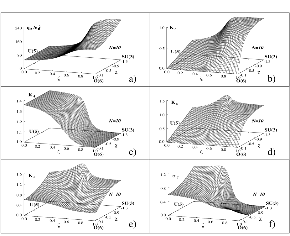
FIG. 2.: a)-e): Shape invariants $q_{2}$ and $K_{3}$ - $K_{6}$ c): The invariant $K_{4}$ also determines the fluctuation $\sigma_{\beta}=K_{4}-1$. f): The fluctuation $\sigma_{\gamma}$. All quantities shown in a)-f) are calculated gridwise over the ECQF parameter space of the IBM for $N=10$ bosons.

REFERENCES

- [1] K. Kumar, Phys. Rev. Lett. 28, 249 (1972).
- [2] D. Cline, Ann. Rev. Nucl. Part. Sci. 36, 683 (1986).
- [3] R.V. Jolos, P. von Brentano, N. Pietralla, and I. Schneider, Nucl. Phys. A 618, 126 (1997).
- [4] Yu.V. Palchikov, P. von Brentano, and R.V. Jolos, Phys. Rev. C 57, 3026 (1998).
- [5] T. Otsuka, and K.-H. Kim, Phys. Rev. C 50, 1768 (1994).
- [6] N. Pietralla, P. von Brentano, R.F. Casten, T. Otsuka, and N.V. Zamfir, Phys. Rev. Lett. 73 2962 (1994).
- [7] N. Pietralla, P. von Brentano, T. Otsuka, and R.F. Casten, Phys. Lett. B 349, 1 (1995).
- [8] N. Pietralla, T. Mizusaki, P. von Brentano, R.V. Jolos, T. Otsuka, and V. Werner, Phys. Rev. C 57, 150 (1998).
- [9] A. Arima and F. Iachello, Phys. Rev. 102, 788 (1975).
- [10] F. Iachello and A. Arima, The Interacting Boson Model (Cambridge University Press, Cambridge, 1987).
- [11] D.D. Warner, and R.F. Casten, Phys. Rev. Lett. 48, 1385 (1982).
- [12] P.O. Lipas, P. Toivonen, and D.D. Warner, Phys. Lett. 155B, 295 (1985).
- [13] D. Bucurescu, private communication.
- [14] R.F. Casten, M. Wilhelm, E. Radermacher, N.V. Zamfir, and P. von Brentano, Phys. Rev. C 57, R1553 (1998).
- [15] N.V. Zamfir, R.F. Casten, M.A. Caprio, C.W. Beausang, R. Krücken, J.R. Novak, J.R. Cooper, G. Cata-Danil, and C.J. Barton, Phys. Rev. C 60, 054312 (1999).
- [16] F. Iachello, N.B. Zamfir, and R.F. Casten, Phys. Rev. Lett. 81, 1191 (1998).
- [17] O. Scholten, unpublished, KVI-63, Groningen.
- [18] J.N. Ginocchio, and M.W. Kirson, Nucl. Phys. A 350, 31 (1980).
- [19] A. Leviatan, A. Novoselsky, and I. Talmi, Phys. Lett. B 172, 144 (1986).