One-body density matrix and momentum distribution in $s$-$p$ and $s$-$d$ shell nuclei

Abstract

Analytical expressions of the one- and two- body terms in the cluster expansion of the one-body density matrix and momentum distribution of the $s$-$p$ and $s$-$d$ shell nuclei with $N=Z$ are derived. They depend on the harmonic oscillator parameter $b$ and the parameter $\beta$ which originates from the Jastrow correlation function. These parameters have been determined by least squares fit to the experimental charge form factors. The inclusion of short-range correlations increases the high momentum component of the momentum distribution, $n({\bf k})$ for all nuclei we have considered while there is an $A$ dependence of $n({\bf k})$ both at small values of $k$ and the high momentum component. The $A$ dependence of the high momentum component of $n({\bf k})$ becomes quite small when the nuclei ²⁴Mg, ²⁸Si and ³²S are treated as $1d$-$2s$ shell nuclei having the occupation probability of the $2s$-state as an extra free parameter in the fit to the form factors.

PACS numbers: 21.45.+v, 21.60.Cs, 21.60.-n, 21.90.+f

I INTRODUCTION

The momentum distribution (MD) is of interest in many research subjects of modern physics, including those referring to helium, electronic, nuclear, and quark systems [1, 2, 3]. In the last two decades, there has been significant effort for the determination of the MD in nuclear matter and finite nucleon systems [4, 5, 6, 7, 8, 9, 10, 11, 12, 13, 14, 15, 16, 17, 18, 19, 20, 21, 22, 23]. MD is related to the cross sections of various kinds of nuclear reactions. Specifically, the interaction of particles with nuclei at high energies, such as (p,2p), (e,e^′p), and (e,e^′) reactions, the nuclear photo-effect, meson absorption by nuclei, the inclusive proton production in proton-nucleus collisions, and even phenomena at low energies such as giant multipole resonances, give significant information about the nucleon MD. The experimental evidence obtained from inclusive and exclusive electron scattering on nuclei established the existence of a high-momentum component for momenta $k>2\ {\rm fm}^{-1}$ [24, 25, 26, 27]. It has been shown that, in principle, mean field theories can not describe correctly MD and density distribution simultaneously [12] and the main features of MD depend little on the effective mean field considered [15]. The reason is that MD is sensitive to short-range and tensor nucleon-nucleon correlations which are not included in the mean field theories. Thus, theoretical approaches, which take into account short range correlations (SRC) due to the character of the nucleon-nucleon forces at small distances, are necessary to be developed.

Zabolitzky and Ey [4], employing the coupled-cluster (or $\exp(S)$) method for the microscopic evaluation of nuclear MD for the ground states of ⁴He and ¹⁶O and using various realistic NN-potentials, showed that the contribution of correlations dominates for momenta beyond $2\ {\rm fm}^{-1}$. A realistic interaction and a many-body approach have been used by Benhar et al [13] for the evaluation of MD of ¹²C, ¹⁶O and ⁴⁰Ca. Their results have yielded a much larger content of the high momentum component with respect to the results obtained within the Hartree-Fock approach or within methods which take into account the effect of correlations phenomenologically.

Bohigas and Stringari [6] and Dal Ri et al [7] evaluated the effect of SRC’s on the one- and two- body densities by developing a low order approximation (LOA) in the framework of Jastrow formalism. They showed that one-body quantities provide an adequate test for the presence of SRC’s in nuclei, which indicates that the independent-particle wave functions cannot reproduce simultaneously the form factor and the MD of a correlated system and also the effect of SRC’s strongly modify the MD by introducing an important contribution in the region $k>2$ fm^-1. Stoitsov et al [17] generalised the model of Jastrow correlations within the LOA of Ref. [28], to heavier nuclei as ¹⁶O, ³⁶Ar, ⁴⁰Ca. Their analytical expressions for the MD show the high momentum tail. They found that there is an A dependence of MD for small values of $k$, while for large values of $k$ the slope of $\log n(k)$ versus $k$ is roughly the same for the above three nuclei as well as for ⁴He. The same behaviour of the MD of protons and neutrons for the $A=3,4$ nuclei has been found earlier by Schiavilla et al [14] performing variational calculations with realistic interactions. MD for the nuclei ⁴He, ¹⁶O and ⁴⁰Ca was also calculated by Traini and Orlandini [11] within a phenomenological model in which dynamical short-range and tensor correlations effects were included. They showed that SRC increase the high momentum component considerably while the tensor correlations do not affect the MD appreciably [11, 29]. In heavy nuclei, the local density approximation was used [16] for the study of the effect of SRC’s in MD and the predictions were in agreement with the results of microscopic calculations in nuclear matter and in light nuclei.

The influence of SRC’s on the MD of nucleons in nuclei has also been evaluated by Müther et al [18] within the Green-function approach assuming a realistic meson-exchange potential for the nucleon-nucleon interaction. Their analysis on ¹⁶O demonstrates that a non-negligible contribution to the MD should be found in partial waves which are unoccupied in the simple shell model. Another approach is to consider the average occupancy of the relevant shell-model orbitals [9]. It has been found that the depletion of such orbitals can be of the order $15\%$ or more for single-particles (SP) states below the Fermi energy [30].

In the various approaches, the MD of the closed shell nuclei ⁴He, ¹⁶O and ⁴⁰Ca as well as of ²⁰⁸Pb and nuclear matter is usually studied. There is no systematic study of the one body density matrix (OBDM) and MD which include both the case of closed and open shell nuclei. This would be helpful in the calculations of the overlap integrals and reactions in that region of nuclei if one wants to go beyond the mean field theories [32]. For that reason, in the present work, we attempt to find some general expressions for the OBDM $\rho({\bf r},{\bf r}^{\prime})$ and MD $n({\bf k})$ which could be used both for closed and open shell nuclei. This work is a continuation of our previous study [31] on the form factors and densities of the $s$-$p$ and $s$-$d$ shell nuclei. The expression of $\rho({\bf r},{\bf r}^{\prime})$ was found, first, using the factor cluster expansion of Clark and co-workers [35, 36, 37] and Jastrow correlation function which introduces SRC for closed shell nuclei and then was extrapolated to the case of $N=Z$ open shell nuclei. $n({\bf k})$ was found by Fourier transform of $\rho({\bf r},{\bf r}^{\prime})$. These expressions are functionals of the harmonic oscillator (HO) orbitals and depend on the HO parameter $b$ and the correlation parameter $\beta$. The values of the parameters $b$ and $\beta$, which we have used for the closed shell nuclei ⁴He, ¹⁶O and ⁴⁰Ca, are the ones which have been determined in Ref. [31] by fit of the theoretical $F_{ch}(q)$, derived with the same cluster expansion, to the experimental one. For the open shell nuclei ¹²C, ²⁴Mg, ²⁸Si and ³²S we provide new values for these parameters, which have been found to give a better fit to the experimental form factors than in our previous analysis [31]. It is found that the high-momentum tail of the MD of all the nuclei we have considered appears for $k>2\ {\rm fm}^{-1}$ and also there is an A dependence of the values of $n(k)$ for $2\ {\rm fm}^{-1}<k<5\ {\rm fm}^{-1}$. This $A$ dependence of MD was first investigated considering ²⁴Mg, ²⁸Si and ³²S as $1d$ shell nuclei. Next we treated the above nuclei as $1d$-$2s$ shell nuclei having the occupation probability of the $2s$ state as an extra free parameter in the fit of the form factors. The $A$ dependence is quite small in the second case.

The paper is organised as follows. In Sec. II the general expressions of the correlated OBDM and MD are derived using a Jastrow correlation function. In Sec. III the analytical expressions of the above quantities for the $s$-$p$ and $s$-$d$ shell nuclei, in the case of the HO orbitals, are given. Numerical results are reported and discussed in Sec. IV, while the summary of the present work is given in Sec. V.

II CORRELATED ONE-BODY DENSITY MATRIX AND MOMENTUM DISTRIBUTION

A nucleus with $A$ nucleons is described by the wave function $\Psi({\bf r}_{1},{\bf r}_{2},...,{\bf r}_{A})$ which depends on $3A$ coordinates as well as on spins and isospins. The evaluation of the single particle characteristics of the system needs the one-body density matrix [33, 34]

$$\rho({\bf r},{\bf r}^{\prime})=\int\Psi^{*}({\bf r},{\bf r}_{2},...,{\bf r}_{A})\ \Psi({\bf r}^{\prime},{\bf r}_{2},\cdots,{\bf r}_{A})\ {\rm d}{\bf r}_{2}\cdots{\rm d}{\bf r}_{A}\ ,$$ (1)

where the integration is carried out over the radius vectors ${\bf r}_{2},\cdots,{\bf r}_{A}$ and summation over spin and isospin variables is implied. $\rho({\bf r},{\bf r}^{\prime})$ can also be represented by the form

$$\rho({\bf r},{\bf r}^{\prime})=\frac{\langle\Psi|{\bf O}_{\bf r\bf r^{\prime}}|\Psi^{\prime}\rangle}{\langle\Psi|\Psi\rangle}\ =\ N\langle\Psi|{\bf O}_{\bf r\bf r^{\prime}}|\Psi^{\prime}\rangle=N\langle{\bf O}_{\bf r\bf r^{\prime}}\rangle\ ,$$ (2)

where $\Psi^{\prime}=\Psi({\bf r}_{1}^{\prime},{\bf r}_{2}^{\prime},...,{\bf r}_{A}^{\prime})$ and $N$ is the normalization factor. The one-body ”density operator” ${\bf O}_{{\bf rr}^{\prime}}$, has the form

$${\bf O}_{{\bf rr}^{\prime}}=\sum_{i=1}^{A}\ \delta({\bf r}_{i}-{\bf r})\delta({\bf r}_{i}^{\prime}-{\bf r}^{\prime})\prod_{j\neq i}^{A}\delta({\bf r}_{j}-{\bf r}_{j}^{\prime})\ .$$ (3)

In the case where the nuclear wave function $\Psi$ can be expressed as a Slater determinant depending on the SP wave functions $\phi_{i}({\bf r})$ we have

$$\rho_{SD}({\bf r},{\bf r}^{\prime})=\sum_{i=1}^{A}\phi_{i}^{*}({\bf r})\phi_{i}({\bf r}^{\prime})$$ (4)

The diagonal elements of the OBDM give the density distribution

$$\rho({\bf r},{\bf r})=\rho({\bf r})\ ,$$ (5)

while the MD is given by the Fourier transform of $\rho({\bf r},{\bf r}^{\prime})$,

$$n({\bf k})=\frac{1}{(2\pi)^{3}}\int\exp[i{\bf k}({\bf r}-{\bf r}^{\prime})]\ \rho({\bf r},{\bf r}^{\prime})\ {\rm d}{\bf r}\ {\rm d}{\bf r}^{\prime}\ .$$ (6)

In the case of a Slater determinant, MD takes the form

$$n_{SD}({\bf k})=\sum_{i=1}^{A}\tilde{\phi}_{i}^{*}({\bf k})\tilde{\phi}_{i}({\bf k})\ ,$$ (7)

where

$$\tilde{\phi}_{i}({\bf k})=\frac{1}{(2\pi)^{3/2}}\int\phi_{i}({\bf r})\exp[i{\bf k}{\bf r}]{\rm d}{\bf r}.$$ (8)

The second moment of the MD is related to the expectation value of the kinetic energy, $\langle{\bf T}\rangle$, by the expression

$$\langle{\bf T}\rangle=\frac{\hbar^{2}}{2m}\int n({\bf k})k^{2}{\rm d}{\bf k}.$$ (9)

A One-body density matrix

If we denote the model operator, which introduces SRC, by $\cal{F}$, an eigenstate $\Phi$ of the model system corresponds to an eigenstate

$$\Psi={\cal F}\Phi$$ (10)

of the true system.

Several restrictions can be made on the model operator $\cal{F}$, as for example, that it depends on (the spins, isospins and) relative coordinates and momenta of the particles in the system, that be a scalar with respect to rotations etc. [38]. Further, it is required that $\cal{F}$ be translationally invariant and symmetrical in its arguments $1\cdots i\cdots A$ and possesses the cluster property. That is if any subset $i_{1}\cdots i_{p}$ of the particles is removed far from the rest $i_{p+1}\cdots i_{A}$, $\cal{F}$ decomposes into a product of two factors, ${\cal F}(1\cdots A)={\cal F}(i_{1}\cdots i_{p})\ {\cal F}(i_{p+1}\cdots i_{A})$ [37]. In the present work $\cal{F}$ is taken to be of the Jastrow type [39],

$${\cal F}=\prod_{i<j}^{A}f(r_{ij})\ ,$$ (11)

where $f(r_{ij})$ is the state-independent correlation function of the form

$$f(r_{ij})=1-\exp[-\beta({\bf r}_{i}-{\bf r}_{j})^{2}]\ .$$ (12)

The correlation function $f(r_{ij})$ goes to 1 for large values of $r_{ij}=\mid{\bf r}_{i}-{\bf r}_{j}\mid$ and it goes to 0 for $r_{ij}\rightarrow 0$. It is obvious that the effect of SRC, introduced by the function $f(r_{ij})$, becomes large when the SRC parameter $\beta$ becomes small and vice versa.

In order to evaluate the correlated one-body density matrix $\rho_{cor}({\bf r},{\bf r}^{\prime})$, we consider, first, the generalized integral

$$I(\alpha)=\langle\Psi|\exp[\alpha I(0){\bf O}_{{\bf rr}^{\prime}}]|\Psi^{\prime}\rangle\ ,$$ (13)

corresponding to the one-body ”density operator” ${\bf O}_{{\bf rr}^{\prime}}$ (given by (3)), from which we have

$$\langle{\bf O}_{{\bf rr}^{\prime}}\rangle=\left[\frac{\partial\ln I(\alpha)}{\partial\alpha}\right]_{\alpha=0}.$$ (14)

For the cluster analysis of equation (14), we consider the sub-product integrals [35, 36, 37], for the sub-systems of the $A$-nucleons system

$$I_{i}(\alpha) = \langle i\mid{\cal F}^{{\dagger}}(r_{1})\exp[\alpha I_{i}(0){\bf o}_{\bf{rr}^{\prime}}(1)]{\cal F}(r_{1}^{\prime})\mid i^{\prime}\rangle\ ,$$ (15)

$$I_{ij}(\alpha) = \langle ij\mid{\cal F}^{{\dagger}}(r_{12})\exp[\alpha I_{ij}(0){\bf o_{rr^{\prime}}}(2)]{\cal F}(r_{12}^{\prime})\mid i^{\prime}j^{\prime}\rangle_{\rm a}\ ,$$ (16)

$$I_{ijk}(\alpha) = \langle ijk\mid{\cal F}^{{\dagger}}(r_{12}){\cal F}^{{\dagger}}(r_{13}){\cal F}^{{\dagger}}(r_{23})\exp[\alpha I_{ijk}(0){\bf o_{rr^{\prime}}}(3)]{\cal F}(r_{12}^{\prime}){\cal F}(r_{13}^{\prime}){\cal F}(r_{23}^{\prime})\mid i^{\prime}j^{\prime}k^{\prime}\rangle_{\rm a}\ ,$$ (17)

. (18)

. (19)

. (20)

$$I_{12\cdots A} = I(\alpha)\ ,$$ (21)

where the operators ${\bf o}_{\bf{rr}^{\prime}}(1)$, ${\bf o}_{\bf{rr}^{\prime}}(2)$, $\ldots$ have the form

$${\bf o_{rr^{\prime}}}(1) = \delta({\bf r}_{1}-{\bf r})\delta({\bf r}_{1}^{\prime}-{\bf r}^{\prime})\ ,$$ (22)

$${\bf o_{rr^{\prime}}}(2) = \delta({\bf r}_{1}-{\bf r})\delta({\bf r}_{1}^{\prime}-{\bf r}^{\prime})\delta({\bf r}_{2}-{\bf r}_{2}^{\prime})+\delta({\bf r}_{2}-{\bf r})\delta({\bf r}_{2}^{\prime}-{\bf r}^{\prime})\delta({\bf r}_{1}-{\bf r}_{1}^{\prime})\ ,$$ (23)

and so on.The factor cluster decomposition of the above integrals, following the factor cluster expansion of Ristig,Ter Low, and Clark [35, 36, 37], gives

$$\langle{\bf O}_{{\bf rr}^{\prime}}\rangle=\langle{\bf O}_{{\bf rr}^{\prime}}\rangle_{1}+\langle{\bf O}_{{\bf rr}^{\prime}}\rangle_{2}+\cdots+\langle{\bf O}_{{\bf rr}^{\prime}}\rangle_{A}\ ,$$ (24)

where

$$\langle{\bf O}_{{\bf rr}^{\prime}}\rangle_{1} = \sum_{i=1}^{A}\left[\frac{\partial\ln I_{i}(\alpha)}{\partial\alpha}\right]_{\alpha=0}\ ,$$ (25)

$$\langle{\bf O}_{{\bf rr}^{\prime}}\rangle_{2} = \sum_{i<j}^{A}\frac{\partial}{\partial\alpha}\left[\ln I_{ij}(\alpha)-\ln I_{i}(\alpha)-\ln I_{j}(\alpha)\right]_{\alpha=0}\ ,$$ (26)

and so on. ${\cal F}(r_{1})$ is chosen to be the identity operator.

Three- and many-body terms will be neglected in the present analysis. Thus, in the two-body approximation, $\rho_{cor}({\bf r},{\bf r}^{\prime})$, defined by Eq. (2), is written

$$\rho_{cor}({\bf r},{\bf r}^{\prime})\approx N[\langle{\bf O}_{{\bf rr}^{\prime}}\rangle_{1}+\langle{\bf O}_{{\bf rr}^{\prime}}\rangle_{22}-\langle{\bf O}_{{\bf rr}^{\prime}}\rangle_{21}]\ ,$$ (27)

where

$$\langle{\bf O}_{{\bf rr}^{\prime}}\rangle_{1}=\sum_{i=1}^{A}\langle i\mid{\bf o}_{{\bf rr}^{\prime}}(1)\mid i^{\prime}\rangle\ ,$$ (28)

$$\langle{\bf O}_{{\bf rr}^{\prime}}\rangle_{22}=\sum_{i<j}^{A}\langle ij\mid{\cal F}^{{\dagger}}(r_{12}){\bf o}_{{\bf rr}^{\prime}}(2){\cal F}(r^{\prime}_{12})\mid i^{\prime}j^{\prime}\rangle_{\rm a},$$ (29)

$$\langle{\bf O}_{{\bf rr}^{\prime}}\rangle_{21}=\sum_{i<j}^{A}\langle ij\mid{\bf o}_{{\bf rr}^{\prime}}(2)\mid i^{\prime}j^{\prime}\rangle_{\rm a}$$ (30)

If the two-body operator ${\cal F}(r^{\prime}_{12})$ is taken to be the correlation function given by Eq. (12), then

$${\cal F}^{{\dagger}}(r_{12}){\bf o}_{{\bf rr}^{\prime}}(2){\cal F}(r^{\prime}_{12})={\bf o}_{{\bf rr}^{\prime}}(2)\left[1-{\rm g}_{1}({\bf r},{\bf r}_{2})-{\rm g}_{2}({\bf r}^{\prime},{\bf r}_{2})+{\rm g}_{3}({\bf r},{\bf r}^{\prime},{\bf r_{2}})\right],$$ (31)

where

$${\rm g}_{1}({\bf r},{\bf r}_{2}) = \exp[-\beta(r^{2}+r_{2}^{2})]\exp[2\beta{\bf rr}_{2}],\quad{\rm g}_{2}({\bf r}^{\prime},{\bf r}_{2})={\rm g}_{1}({\bf r}^{\prime},{\bf r}_{2}),$$ (32)

$${\rm g}_{3}({\bf r},{\bf r}^{\prime},{\bf r}_{2}) = \exp[-\beta(r^{2}+{r^{\prime}}^{2})]\exp[-2\beta r_{2}^{2}]\exp[2\beta({\bf r}+{\bf r}^{\prime}){\bf r}_{2}]$$ (33)

and the term $\langle{\bf O}_{\bf rr^{\prime}}\rangle_{22}$ is written

$$\langle{\bf O}_{\bf rr^{\prime}}\rangle_{22}=\langle{\bf O}_{\bf rr^{\prime}}\rangle_{21}-O_{22}({\bf r},{\bf r}^{\prime},{\rm g}_{1})-O_{22}({\bf r},{\bf r}^{\prime},{\rm g}_{2})+O_{22}({\bf r},{\bf r}^{\prime},{\rm g}_{3})\ ,$$ (34)

where

$$O_{22}({\bf r},{\bf r}^{\prime},{\rm g}_{\ell})=\sum_{i<j}^{A}\langle ij\mid{\bf o}_{{\bf rr}^{\prime}}(2){\rm g}_{\ell}({\bf r},{\bf r}^{\prime},{\bf r}_{2})\mid i^{\prime}j^{\prime}\rangle_{\rm a}\ ,\quad\ell=1,2,3\ .$$ (35)

Thus, $\rho_{cor}({\bf r},{\bf r}^{\prime})$ takes the form

$$\rho_{cor}({\bf r},{\bf r}^{\prime})\approx N[\langle{\bf O}_{{\bf rr}^{\prime}}\rangle_{1}-O_{22}({\bf r},{\bf r}^{\prime},{\rm g}_{1})-O_{22}({\bf r},{\bf r}^{\prime},{\rm g}_{2})+O_{22}({\bf r},{\bf r}^{\prime},{\rm g}_{3})]\ .$$ (36)

This is also expressed in the following form

$$\rho_{cor}({\bf r},{\bf r}^{\prime}) \approx N\left[\rho_{SD}({\bf r},{\bf r}^{\prime})+\int\left[-{\rm g}_{1}({\bf r},{\bf r}_{2})-{\rm g}_{2}({\bf r}^{\prime},{\bf r}_{2})+{\rm g}_{3}({\bf r},{\bf r}^{\prime},{\bf r}_{2})\right]\right.$$ (39)

$$\times\left.\left[\rho_{SD}({\bf r},{\bf r}^{\prime})\rho_{SD}({\bf r}_{2},{\bf r}_{2})-\rho_{SD}({\bf r},{\bf r}_{2})\rho_{SD}({\bf r}_{2},{\bf r}^{\prime})\right]{\rm d}{\bf r}_{2}\frac{}{}\right],$$

where $\rho_{SD}({\bf r},{\bf r^{\prime}})$ is the uncorrelated OBDM associated with the Slater determinant.

It should be noted that a similar expression for $\rho_{cor}({\bf r},{\bf r}^{\prime})$, given by Eq. (39), was derived by Gaudin et al. [28] in the framework of LOA. Their expansion contains one- and two-body terms and a part of the three-body term which was chosen so that the normalization of the wave function was preserved. Expression (39) of the present work has only one- and two-body terms and the normalization of the wave function is preserved by the normalization factor $N$.

In the above expression of $\rho_{cor}({\bf r},{\bf r}^{\prime})$, the one-body contribution to the OBDM is well known and is given by the equation

$$\langle{\bf O}_{{\bf rr}^{\prime}}\rangle_{1}=\rho_{SD}({\bf r},{\bf r}^{\prime})=\frac{1}{\pi}\sum_{nl}\eta_{nl}(2l+1)\phi^{*}_{nl}(r)\phi_{nl}(r^{\prime})P_{l}(\cos\omega_{rr^{\prime}})$$ (40)

where $\eta_{nl}$ are the occupation probabilities of the states $nl$ (0 or 1 in the case of closed shell nuclei) and $\phi_{nl}(r)$ is the radial part of the SP wave function and $\omega_{rr^{\prime}}$ the angle between the vectors ${\bf r}$ and ${\bf r}^{\prime}$.

The term $O_{22}({\bf r},{\bf r}^{\prime},{\rm g}_{\ell})$, performing the spin-isospin summation and the angular integration, takes the general form

$$O_{22}({\bf r},{\bf r}^{\prime},{\rm g}_{\ell}) = 4\sum_{n_{i}l_{i},n_{j}l_{j}}\eta_{n_{i}l_{i}}\eta_{n_{j}l_{j}}(2l_{i}+1)(2l_{j}+1)$$ (42)

$$\times\left[4A_{n_{i}l_{i}n_{j}l_{j}}^{n_{i}l_{i}n_{j}l_{j},0}({\bf r},{\bf r}^{\prime},{\rm g}_{\ell})-\sum_{k=0}^{l_{i}+l_{j}}\langle l_{i}0l_{j}0\mid k0\rangle^{2}A_{n_{i}l_{i}n_{j}l_{j}}^{n_{j}l_{j}n_{i}l_{i},k}({\bf r},{\bf r}^{\prime},{\rm g}_{\ell})\right],\ \ell=1,2,3,$$

where

$$A_{n_{1}l_{1}n_{2}l_{2}}^{n_{3}l_{3}n_{4}l_{4},k}({\bf r},{\bf r}^{\prime},{\rm g}_{1}) = \frac{1}{4\pi}\phi^{*}_{n_{1}l_{1}}(r)\ \phi_{n_{3}l_{3}}(r^{\prime})\ \exp[-\beta r^{2}]\ P_{l_{3}}(\cos\omega_{rr^{\prime}})$$ (44)

$$\times\int_{0}^{\infty}\phi^{*}_{n_{2}l_{2}}(r_{2})\ \phi_{n_{4}l_{4}}(r_{2})\ \exp[-\beta r_{2}^{2}]\ i_{k}(2\beta rr_{2})\ r_{2}^{2}\ {\rm d}r_{2},$$

and the matrix element $A_{n_{1}l_{1}n_{2}l_{2}}^{n_{3}l_{3}n_{4}l_{4},k}({\bf r},{\bf r}^{\prime},{\rm g}_{2})$ can be found from (44) replacing ${\bf r}\longleftrightarrow{\bf r}^{\prime}$ and $n_{1}l_{1}\longleftrightarrow n_{3}l_{3}$ while the matrix element corresponding to the factor ${\rm g}_{3}$ is

$$A_{n_{1}l_{1}n_{2}l_{2}}^{n_{3}l_{3}n_{4}l_{4},k}({\bf r},{\bf r}^{\prime},{\rm g}_{3}) = \frac{1}{4\pi}\phi^{*}_{n_{1}l_{1}}(r)\ \phi_{n_{3}l_{3}}(r^{\prime})\ \exp[-\beta(r^{2}+r^{\prime 2})]\ \Omega_{l_{1}l_{3}}^{k}(\omega_{rr^{\prime}})\times$$ (46)

$$\int_{0}^{\infty}\phi^{*}_{n_{2}l_{2}}(r_{2})\ \phi_{n_{4}l_{4}}(r_{2})\ \exp[-2\beta r_{2}^{2}]\ i_{k}(2\beta|{\bf r}+{\bf r}^{\prime}|r_{2})\ r_{2}^{2}\ {\rm d}r_{2},$$

In Eqs. (44) and (46) the modified spherical Bessel function, $i_{k}(z)$, comes from the expansion of the exponential function $\exp[2\beta{\bf x}_{1}{\bf x}_{2}]$ of the factors ${\rm g}_{\ell}$ in spherical harmonics, that is

$\displaystyle\exp[2\beta{\bf x}_{1}{\bf x}_{2}]=4\pi\sum_{km_{k}}i_{k}(2\beta x_{1}x_{2})Y^{*}_{km_{k}}(\Omega_{1})Y_{km_{k}}(\Omega_{2}),$

while the factor $\Omega_{l_{1}l_{3}}^{k}(\omega_{rr^{\prime}})$ which depends on the directions of ${\bf r}$ and ${\bf r}^{\prime}$ is,

$$\Omega_{l_{1}l_{3}}^{k}(\omega_{rr^{\prime}})=\sum_{m_{1},m_{3}}\frac{\langle l_{1}-m_{1}l_{3}m_{3}\mid k0\rangle}{\langle l_{1}0l_{3}0\mid k0\rangle}\left(\frac{(l_{1}-m_{1})!}{(l_{1}+m_{1})!}\frac{(l_{3}-m_{3})!}{(l_{3}+m_{3})!}\right)^{\frac{1}{2}}\ P_{l_{1}}^{m_{1}}(\cos\omega_{r})\ P_{l_{3}}^{m_{3}}(\cos\omega_{r^{\prime}})\ ,$$ (47)

where $\omega_{r}$ and $\omega_{r^{\prime}}$ are the angles between the vectors ${\bf r},\ {\bf r}+{\bf r}^{\prime}$ and ${\bf r}^{\prime},\ {\bf r}+{\bf r}^{\prime}$, respectively. The final expression of $\Omega_{l_{1}l_{3}}^{k}(\omega_{rr^{\prime}})$ depends on $\omega_{rr^{\prime}}$, the angle between the vectors ${\bf r}$ and ${\bf r}^{\prime}$.

The expression of the term $O_{22}({\bf r},{\bf r}^{\prime},{\rm g}_{\ell})$ depends on the SP wave functions and so it is suitable to be used for analytical calculations with the HO orbitals and in principle for numerical calculations with more realistic SP orbitals. Expressions (40) and (42) were derived for the closed shell nuclei with $N=Z$, where $\eta_{nl}$ is 0 or 1. For the open shell nuclei (with $N=Z$) we use the same expressions, where now $0\leq\eta_{nl}\leq 1$. In this way the mass dependence of the correlation parameter $\beta$ and the OBDM or MD can be studied.

Finally, using the known values of the Clebsch-Gordan coefficients, Eq. (42), for the case of $s$-$p$ and $s$-$d$ shell nuclei, takes the form

$$O_{22}({\bf r},{\bf r}^{\prime},{\rm g}_{\ell})=$$ (48)

$$4\left[\frac{}{}3A_{0000}^{0000,0}({\bf r},{\bf r}^{\prime},{\rm g}_{\ell})\eta_{1s}^{2}+\left[33A_{0101}^{0101,0}({\bf r},{\bf r}^{\prime},{\rm g}_{\ell})-6A_{0101}^{0101,2}({\bf r},{\bf r}^{\prime},{\rm g}_{\ell})\right]\eta_{1p}^{2}+3A_{1010}^{1010,0}({\bf r},{\bf r}^{\prime},{\rm g}_{\ell})\eta_{2s}^{2}\right.$$ (49)

(50)

$$+\left[95A_{0202}^{0202,0}({\bf r},{\bf r}^{\prime},{\rm g}_{\ell})-\frac{50}{7}A_{0202}^{0202,2}({\bf r},{\bf r}^{\prime},{\rm g}_{\ell})-\frac{90}{7}A_{0202}^{0202,4}({\bf r},{\bf r}^{\prime},{\rm g}_{\ell})\right]\eta_{1d}^{2}$$ (51)

(52)

$$+\left[12A_{0001}^{0001,0}({\bf r},{\bf r}^{\prime},{\rm g}_{\ell})+12A_{0100}^{0100,0}({\bf r},{\bf r}^{\prime},{\rm g}_{\ell})-3A_{0001}^{0100,1}({\bf r},{\bf r}^{\prime},{\rm g}_{\ell})-3A_{0100}^{0001,1}({\bf r},{\bf r}^{\prime},{\rm g}_{\ell})\right]\eta_{1s}\eta_{1p}$$ (53)

(54)

$$+\left[20A_{0002}^{0002,0}({\bf r},{\bf r}^{\prime},{\rm g}_{\ell})+20A_{0200}^{0200,0}({\bf r},{\bf r}^{\prime},{\rm g}_{\ell})-5A_{0002}^{0200,2}({\bf r},{\bf r}^{\prime},{\rm g}_{\ell})-5A_{0200}^{0002,2}({\bf r},{\bf r}^{\prime},{\rm g}_{\ell})\right]\eta_{1s}\eta_{1d}$$ (55)

(56)

$$+\left[4A_{0010}^{0010,0}({\bf r},{\bf r}^{\prime},{\rm g}_{\ell})+4A_{1000}^{1000,0}({\bf r},{\bf r}^{\prime},{\rm g}_{\ell})-A_{0010}^{1000,0}({\bf r},{\bf r}^{\prime},{\rm g}_{\ell})-A_{1000}^{0010,0}({\bf r},{\bf r}^{\prime},{\rm g}_{\ell})\right]\eta_{1s}\eta_{2s}$$ (57)

(58)

$$+\left[60A_{0102}^{0102,0}({\bf r},{\bf r}^{\prime},{\rm g}_{\ell})+60A_{0201}^{0201,0}({\bf r},{\bf r}^{\prime},{\rm g}_{\ell})-6A_{0102}^{0201,1}({\bf r},{\bf r}^{\prime},{\rm g}_{\ell})-6A_{0201}^{0102,1}({\bf r},{\bf r}^{\prime},{\rm g}_{\ell})\right.$$ (59)

(60)

$$-\left.9A_{0102}^{0201,3}({\bf r},{\bf r}^{\prime},{\rm g}_{\ell})-9A_{0201}^{0102,3}({\bf r},{\bf r}^{\prime},{\rm g}_{\ell})\right]\eta_{1p}\eta_{1d}$$ (61)

(62)

$$+\left[12A_{0110}^{0110,0}({\bf r},{\bf r}^{\prime},{\rm g}_{\ell})+12A_{1001}^{1001,0}({\bf r},{\bf r}^{\prime},{\rm g}_{\ell})-3A_{0110}^{1001,1}({\bf r},{\bf r}^{\prime},{\rm g}_{\ell})-3A_{1001}^{0110,1}({\bf r},{\bf r}^{\prime},{\rm g}_{\ell})\right]\eta_{1p}\eta_{2s}$$ (63)

(64)

$$\left.+\left[20A_{0210}^{0210,0}({\bf r},{\bf r}^{\prime},{\rm g}_{\ell})+20A_{1002}^{1002,0}({\bf r},{\bf r}^{\prime},{\rm g}_{\ell})-5A_{0210}^{1002,2}({\bf r},{\bf r}^{\prime},{\rm g}_{\ell})-5A_{1002}^{0210,2}({\bf r},{\bf r}^{\prime},{\rm g}_{\ell})\right]\eta_{{}_{1d}}\eta_{2s}\frac{}{}\right].$$ (65)

It should be noted that Eqs. (42) and (65) are also valid for the cluster expansion of the density distribution and the form factor as it has been found in ref. [31] and also in the cluster expansion of the MD. The only difference is the expressions of the matrix elements $A$.

B Momentum distribution

The MD for the above mentioned nuclei can be found either by following the same cluster expansion or by taking the Fourier transform of $\rho({\bf r},{\bf r}^{\prime})$ given by (36). In both cases the correlated momentum distribution takes the form

$$n_{cor}({\bf k})\approx N\left[\langle{\bf\tilde{O}}_{\bf k}\rangle_{1}-2\tilde{O}_{22}({\bf k},{\rm g}_{1})+\tilde{O}_{22}({\bf k},{\rm g}_{3})\right]\ ,$$ (66)

where

$$\langle{\bf\tilde{O}}_{\bf k}\rangle_{1}=n_{SD}({\bf k})=\sum_{i=1}^{A}\tilde{\phi}_{i}^{*}({\bf k})\tilde{\phi}_{i}({\bf k}).$$ (67)

The term $\tilde{O}_{22}({\bf k},{\rm g}_{\ell})$, as in the case of OBDM, is given again by the right-hand side of Eqs. (42) and (65) replacing the matrix elements $A_{n_{1}l_{1}n_{2}l_{2}}^{n_{3}l_{3}n_{4}l_{4},k}({\bf r},{\bf r}^{\prime},{\rm g}_{\ell})$, defined by Eqs. (44) and (46), by the Fourier transform of them, that is by the matrix elements

$$\tilde{A}_{n_{1}l_{1}n_{2}l_{2}}^{n_{3}l_{3}n_{4}l_{4},k}({\bf k},{\rm g}_{\ell})=\frac{1}{(2\pi)^{3}}\int A_{n_{1}l_{1}n_{2}l_{2}}^{n_{3}l_{3}n_{4}l_{4},k}({\bf r},{\bf r}^{\prime},{\rm g}_{\ell})\exp[i{\bf k}({\bf r}-{\bf r}^{\prime})]{\rm d}{\bf r}{\rm d}{\bf r}^{\prime},\quad\ell=1,3\ .$$ (68)

As in the case of the OBDM, expression (66) is suitable for the study of the MD for the $s$-$p$ and $s$-$d$ shell nuclei and also for the study of the mass dependence of the kinetic energy of these nuclei. The mean value of the kinetic energy has the form

$$\langle{\bf T}\rangle=N[\langle{\bf T}\rangle_{1}-2T_{22}({\rm g}_{1})+T_{22}({\rm g}_{3})]\ ,$$ (69)

where

$$\langle{\bf T}\rangle_{1}=\frac{\hbar^{2}}{2m}\int k^{2}n_{SD}({\bf k}){\rm d}{\bf k}\ ,\quad T_{22}({\rm g}_{\ell})=\frac{\hbar^{2}}{2m}\int k^{2}\tilde{O}_{22}({\bf k},{\rm g}_{\ell}){\rm d}{\bf k}\ ,\quad\ell=1,3\ .$$ (70)

III ANALYTICAL EXPRESSIONS

In the case of the HO wave functions, with radial part in coordinate and momentum space,

$$\phi_{nl}(r) = N_{nl}b^{-3/2}r_{b}^{l}L_{n}^{l+\frac{1}{2}}\left(r_{b}^{2}\right){\rm e}^{-r_{b}^{2}/2}\ ,\,\,r_{b}=r/b\ ,$$ (71)

$$\tilde{\phi}_{nl}(k) = i^{l}(-1)^{n+l}N_{nl}b^{3/2}k_{b}^{l}L_{n}^{l+\frac{1}{2}}\left(k_{b}^{2}\right)\ {\rm e}^{-k_{b}^{2}/2}\ ,\,\,k_{b}=kb\ ,$$ (72)

where

$\displaystyle N_{nl}=\left(\frac{2n!}{\Gamma(n+l+\frac{3}{2})}\right)^{1/2},$

analytical expressions of the one-body terms, $\langle{\bf O_{rr^{\prime}}}\rangle_{1}$ and $\langle{\bf\tilde{O}}_{\bf k}\rangle_{1}$ as well as of the matrix elements $A_{n_{1}l_{1}n_{2}l_{2}}^{n_{3}l_{3}n_{4}l_{4},k}({\bf r},{\bf r}^{\prime},{\rm g}_{\ell})$ and $\tilde{A}_{n_{1}l_{1}n_{2}l_{2}}^{n_{3}l_{3}n_{4}l_{4},k}({\bf k},{\rm g}_{\ell})$, which have been defined in Sec. II, can be found. From these expressions, the analytical expressions of the terms $O_{22}({\bf r},{\bf r}^{\prime},{\rm g}_{\ell})$ and $\tilde{O}_{22}({\bf k},{\rm g}_{\ell})$, defined by Eq. (65), can also be found.

The expressions of the one-body terms, $\langle{\bf O_{rr^{\prime}}}\rangle_{1}$ and $\langle{\bf\tilde{O}}_{\bf k}\rangle_{1}$, have the forms

$$\langle{\bf O}_{{\bf rr}^{\prime}}\rangle_{1}=\rho_{SD}({\bf r},{\bf r}^{\prime}) = \frac{2}{\pi^{3/2}b^{3}}\left[\frac{}{}2\eta_{1s}+3\eta_{2s}-2\eta_{2s}(r_{b}^{2}+{r_{b}^{\prime}}^{2})+4\eta_{1p}r_{b}r_{b}^{\prime}\cos\omega_{rr^{\prime}}\right.$$ (75)

$$+\left.\frac{4}{3}[\eta_{2s}+\eta_{1d}(3\cos^{2}\omega_{rr^{\prime}}-1)r_{b}^{2}{r_{b}^{\prime}}^{2}]\frac{}{}\right]\exp[-(r_{b}^{2}+{r_{b}^{\prime}}^{2})/2]$$

$$\langle{\bf\tilde{O}}_{\bf k}\rangle_{1}=n_{SD}({\bf k})=\frac{2b^{3}}{\pi^{3/2}}\exp[-k_{b}^{2}]\ \sum_{k=0}^{2}C_{2k}k_{b}^{2k}\ ,$$ (76)

where the coefficients $C_{2k}$ are

$$C_{0}=2\eta_{1s}+3\eta_{2s}\ ,\quad C_{2}=4(\eta_{1p}-\eta_{2s})\ ,\quad C_{4}=\frac{4}{3}(2\eta_{1d}+\eta_{2s})\ .$$ (77)

The analytical expressions of the matrix element $A_{n_{1}l_{1}n_{2}l_{2}}^{n_{3}l_{3}n_{4}l_{4},k}({\bf r},{\bf r}^{\prime},{\rm g}_{\ell})$ $(\ell=1,3)$ have the form

$$A_{n_{1}l_{1}n_{2}l_{2}}^{n_{3}l_{3}n_{4}l_{4},k}({\bf r},{\bf r}^{\prime},{\rm g}_{1}) = B_{0}\ b^{-3}y^{k}\ r_{b}^{k+l_{1}}{r^{\prime}_{b}}^{l_{3}}\ L_{n_{1}}^{l_{1}+\frac{1}{2}}(r_{b}^{2})\ L_{n_{3}}^{l_{3}+\frac{1}{2}}({r^{\prime}_{b}}^{2})\exp\left[-\frac{1+3y}{2(1+y)}r_{b}^{2}-\frac{1}{2}{r^{\prime}_{b}}^{2}\right]$$ (79)

$$\times P_{l_{3}}(\cos\omega_{rr^{\prime}})\sum_{w_{2}=0}^{n_{2}}\sum_{w_{4}=0}^{n_{4}}B_{w_{2}w_{4}}(y)\ L_{\frac{1}{2}(l_{2}+l_{4}-k)+w_{2}+w_{4}}^{k+\frac{1}{2}}\left(\frac{-y^{2}}{1+y}r_{b}^{2}\right)\ ,$$

and

$$A_{n_{1}l_{1}n_{2}l_{2}}^{n_{3}l_{3}n_{4}l_{4},k}({\bf r},{\bf r}^{\prime},{\rm g}_{3}) = B_{0}\ b^{-3}y^{k}\mid{\bf r}_{b}+{\bf r}^{\prime}_{b}\mid^{k}r_{b}^{l_{1}}{r^{\prime}_{b}}^{l_{3}}\ L_{n_{1}}^{l_{1}+\frac{1}{2}}(r_{b}^{2})\ L_{n_{3}}^{l_{3}+\frac{1}{2}}({r^{\prime}_{b}}^{2})\Omega_{l_{1}l_{3}}^{k}(\omega_{rr^{\prime}})$$ (82)

$$\times\exp\left[-\frac{1+2y}{2}(r_{b}^{2}+{r^{\prime}_{b}}^{2})\right]\exp\left[\frac{y^{2}}{1+2y}({\bf r}_{b}+{\bf r}^{\prime}_{b})^{2}\right]$$

$$\times\sum_{w_{2}=0}^{n_{2}}\sum_{w_{4}=0}^{n_{4}}B_{w_{2}w_{4}}(2y)\ L_{\frac{1}{2}(l_{2}+l_{4}-k)+w_{2}+w_{4}}^{k+\frac{1}{2}}\left(-\frac{y^{2}}{1+2y}({\bf r}_{b}+{\bf r}^{\prime}_{b})^{2}\right)$$

where $y=\beta b^{2}$ and

$$B_{0}=\frac{1}{16\sqrt{\pi}}\left(\prod_{i=1}^{4}N_{n_{i}l_{i}}\right),$$ (83)

$$B_{w_{2}w_{4}}(z)=[\frac{1}{2}(l_{2}+l_{4}-k)+w_{2}+w_{4}]!\prod_{i=2,4}\frac{(-1)^{w_{i}}}{w_{i}!}\left(\!\!\begin{array}[]{c}n_{i}+l_{i}+\frac{1}{2}\\ n_{i}-w_{i}\end{array}\!\!\right)(1+z)^{-\frac{1}{2}l_{i}-w_{i}-\frac{1}{2}(3+k)}\ ,$$ (84)

while the one corresponding to the factor ${\rm g}_{2}$ can be found from (79) replacing $r_{b}\longleftrightarrow r^{\prime}_{b}$ and $n_{1}l_{1}\longleftrightarrow n_{3}l_{3}$.

The substitution of $A_{n_{1}l_{1}n_{2}l_{2}}^{n_{3}l_{3}n_{4}l_{4},k}({\bf r},{\bf r}^{\prime},{\rm g}_{\ell})$ to the expression of $O_{22}({\bf r},{\bf r}^{\prime},g_{\ell})$ which is given by Eq. (65) leads to the analytical expression of the two-body term of the OBDM, which is of the form

$$O_{22}({\bf r}_{b},{\bf r}_{b}^{\prime}) = f_{1}(r_{b},r_{b}^{\prime},\cos\omega_{rr^{\prime}})\exp\left[-\frac{1+3y}{2(1+y)}r_{b}^{2}-\frac{1}{2}{r_{b}^{\prime}}^{2}\right]$$ (87)

$$+f_{1}(r_{b}^{\prime},r_{b},\cos\omega_{rr^{\prime}})\exp\left[-\frac{1+3y}{2(1+y)}{r_{b}^{\prime}}^{2}-\frac{1}{2}r_{b}^{2}\right]$$

$$+f_{3}(r_{b},r_{b}^{\prime},\cos\omega_{rr^{\prime}})\exp\left[-\frac{1+2y}{2}(r_{b}^{2}+{r_{b}^{\prime}}^{2})\right]\exp\left[\frac{y^{2}}{1+2y}({\bf r}_{b}+{\bf r}_{b}^{\prime})^{2}\right],$$

where $f_{\ell}(r_{b},r_{b}^{\prime},\cos\omega_{rr^{\prime}}),\ (\ell=1,3)$ are polynomials of $r_{b},\ r_{b}^{\prime}$ and $\cos\omega_{rr^{\prime}}$ which depend also on $y=\beta b^{2}$ and the occupation probabilities of the various states.

The corresponding analytical expressions of the matrix elements $\tilde{A}_{n_{1}l_{1}n_{2}l_{2}}^{n_{3}l_{3}n_{4}l_{4},k}({\bf k},{\rm g}_{\ell})$, $(\ell=1,3)$ which contribute to the two-body term of the MD were found substituting $\phi_{nl}(r)$ with that of the HO wave function into Eq. (68). The expression of $\tilde{A}_{n_{1}l_{1}n_{2}l_{2}}^{n_{3}l_{3}n_{4}l_{4},k}({\bf k},{\rm g}_{1})$, which can be found easily, has the form

$$\tilde{A}_{n_{1}l_{1}n_{2}l_{2}}^{n_{3}l_{3}n_{4}l_{4},k}({\bf k},{\rm g}_{1}) = B_{0}b^{3}(-1)^{n_{3}}k_{b}^{2l_{3}}\ L_{n_{3}}^{l_{3}+\frac{1}{2}}\left(k_{b}^{2}\right)\ \exp\left[-\frac{1+2y}{1+3y}k_{b}^{2}\right]$$ (93)

$$\times\sum_{w_{1}=0}^{n_{1}}\sum_{w_{2}=0}^{n_{2}}\sum_{w_{4}=0}^{n_{4}}\sum_{t=0}^{\frac{1}{2}(l_{2}+l_{4}-k)+w_{2}+w_{4}}\tilde{B}_{w_{2}w_{4}t}(y)\left[\frac{1}{2}(l_{1}-l_{3}+k)+w_{1}+t)\right]!$$

$$\times\frac{(-1)^{w_{1}}}{w_{1}!}\left(\begin{array}[]{c}n_{1}+l_{1}+\frac{1}{2}\\ n_{1}-w_{1}\end{array}\right)2^{\frac{1}{2}(l_{1}-l_{3})+w_{1}}\ \ (1+y)^{\frac{1}{2}(l_{1}+l_{3}-l_{2}-l_{4})+w_{1}-w_{2}-w_{4}}$$

$$\times(1+3y)^{-\frac{1}{2}(3+l_{1}+l_{3}+k)-w_{1}-t}\ L_{\frac{1}{2}(l_{1}-l_{3}+k)+w_{1}+t}^{l_{3}+\frac{1}{2}}\left(\frac{1+y}{2(1+3y)}k_{b}^{2}\right),$$

where

$$\tilde{B}_{w_{2}w_{4}t}(y) = (\sqrt{2}y)^{k+2t}\left[\frac{1}{2}(1+l_{2}+l_{4}+k)+w_{2}+w_{4}\right]!\left[\frac{k-l_{2}-l_{4}}{2}-w_{2}-w_{4}\right]_{t}$$ (97)

$$\times\frac{1}{(k+t+\frac{1}{2})!}\prod_{i=2,4}\frac{(-1)^{w_{i}+t}}{w_{i}!t!}\left(\!\!\begin{array}[]{c}n_{i}+l_{i}+\frac{1}{2}\\ n_{i}-w_{i}\end{array}\!\!\right).$$

The expression of $\tilde{A}_{n_{1}l_{1}n_{2}l_{2}}^{n_{3}l_{3}n_{4}l_{4},k}({\bf k},{\rm g}_{3})$ is more complicated. It has the the general form

$$\tilde{A}_{n_{1}l_{1}n_{2}l_{2}}^{n_{3}l_{3}n_{4}l_{4},k}({\bf k},{\rm g}_{3}) = \frac{2}{\sqrt{\pi}}B_{0}b^{3}\exp\left[-\frac{k_{b}^{2}}{1+2y}\right]\sum_{w_{2}=0}^{n_{2}}\sum_{w_{4}=0}^{n_{4}}\sum_{t=0}^{\frac{1}{2}(l_{2}+l_{4}-k)+w_{2}+w_{4}}\tilde{B}_{w_{2}w_{4}t}(y)$$ (99)

$$\times(1+2y)^{-\frac{1}{2}(3+l_{2}+l_{4}+k)-w_{2}-w_{4}-t}I_{n_{1}l_{1}}^{n_{3}l_{3},k}(k_{b})\ .$$

The general expression of the quantity $I_{n_{1}l_{1}}^{n_{3}l_{3},k}(k_{b})$ is quite complicated. For that reason we calculated it for various cases which are needed for the $s$-$p$ and $s$-$d$ shell nuclei. The various cases and the corresponding expressions of $I_{n_{1}l_{1}}^{n_{3}l_{3},k}(k_{b})$ are given bellow.

1 Case 1: $n_{1}l_{1}=n_{3}l_{3}$ and $k=0$

$$I_{n_{1}l_{1}}^{n_{1}l_{1},0}(k_{b}) = \sum_{\rho=0}^{[l_{1}/2]}\sum_{\sigma=0}^{n_{1}}\sum_{\tau=0}^{\rho+\sigma}\sum_{\nu=0}^{2(\rho+\sigma-\tau)}\sum_{\alpha=0}^{l_{1}-2\rho}\sum_{\mu=0}^{n_{1}-\sigma}\sum_{w_{1}=0}^{n_{1}-\sigma-\mu}\sum_{w_{3}=0}^{\mu}\frac{(-1)^{\rho+\alpha+\tau+w_{1}+w_{3}}}{n_{1}!\rho!\sigma!w_{1}!w_{3}!}L_{\alpha+w_{1}+\tau+\nu}^{\frac{1}{2}}\left(\frac{k_{b}^{2}}{1+2y}\right)$$ (115)

$$\times\left(\!\!\begin{array}[]{c}l_{1}-2\rho\\ \alpha\end{array}\!\!\right)\left(\!\!\begin{array}[]{c}\rho+\sigma\\ \tau\end{array}\!\!\right)\left(\!\!\begin{array}[]{c}2(\rho+\sigma-\tau)\\ \nu\end{array}\!\!\right)\left(\!\!\begin{array}[]{c}n_{1}+\sigma-\mu\\ n_{1}-\sigma-\mu-w_{1}\end{array}\!\!\right)\left(\!\!\begin{array}[]{c}\mu+l_{1}-\frac{1}{2}\\ \mu-w_{3}\end{array}\!\!\right)$$

$$\times\frac{(\alpha+w_{1}+\tau+\nu)!}{2\tau+1}\frac{(2l_{1}-2\rho)!(n_{1}+l_{1}+\frac{1}{2})!(l_{1}+w_{3}+t+2\sigma-\alpha-\tau-\nu+\frac{1}{2})!}{(l_{1}-\rho)!(l_{1}-2\rho)!(\sigma+l_{1}+\frac{1}{2})!}$$

$$\times 2^{-l_{1}+w_{1}+w_{3}+t+2\tau}(1+2y)^{l_{1}-w_{1}+w_{3}+t+2(\sigma-\alpha-\tau-\nu)}(1+4y)^{-\frac{3}{2}-l_{1}-w_{3}-t-2\sigma+\alpha+\tau+\nu}\ .$$

2 Case 2: $n_{1}l_{1}=n_{3}l_{3}=01$ and $k=2$

$$I_{01}^{01,2}(k_{b}) = 2^{1+t}\left(\frac{5}{2}+t\right)!(1+2y)^{2+t}(1+4y)^{-\frac{7}{2}-t}\ .$$ (116)

3 Case 3: $n_{1}l_{1}=n_{3}l_{3}=02$ and $k=2,4$

$$I_{02}^{02,k}(k_{b}) = 2^{\frac{k}{2}+t}(1+2y)^{1+t}(1+4y)^{-\frac{7}{2}-t}$$ (118)

$$\times\left[\left(\frac{5+k}{2}+t\right)!(1+2y)^{1+\frac{k}{2}}(1+4y)^{-\frac{k}{2}}-\delta_{2k}\frac{7}{3}\left(\frac{5}{2}+t\right)!L_{1}^{\frac{1}{2}}\left(\frac{k_{b}^{2}}{1+2y}\right)\right].$$

4 Case 4: $n_{1}l_{1}\neq n_{3}l_{3}$ and $l_{1}=0$ or/and $l_{3}=0$

$$I_{n_{1}l_{1}}^{n_{3}l_{3},k}(k_{b}) = \sum_{w_{1}=0}^{n_{1}}\sum_{w_{3}=0}^{n_{3}}\sum_{\rho_{1}=0}^{[l_{1}/2]}\sum_{\rho_{3}=0}^{[l_{3}/2]}\sum_{\tau_{1}=0}^{l_{1}-2\rho_{1}}\sum_{\tau_{3}=0}^{l_{3}-2\rho_{3}}\sum_{\sigma_{1}=0}^{\rho_{1}+w_{1}}\sum_{\sigma_{3}=0}^{\rho_{3}+w_{3}}\sum_{\nu=0}^{\rho_{1}+\rho_{3}+w_{1}+w_{3}-\sigma_{1}-\sigma_{3}}\frac{1+(-1)^{\tau_{1}+\tau_{3}+\sigma_{1}+\sigma_{3}}}{2(\tau_{1}+\tau_{3}+\sigma_{1}+\sigma_{3}+1)}$$ (131)

$$\times\left[\prod_{i=1,3}(-1)^{\rho_{i}+w_{i}+\tau_{3}+\sigma_{3}}\frac{2^{\frac{1}{2}k-l_{i}+\sigma_{i}+t}(2l_{i}-2\rho_{i})!}{w_{i}!(l_{i}-\rho_{i})!(l_{i}-2\rho_{i})!}\left(\!\!\begin{array}[]{c}n_{i}+l_{i}+\frac{1}{2}\\ n_{i}-w_{i}\end{array}\!\!\right)\left(\!\!\begin{array}[]{c}l_{i}-2\rho_{i}\\ \tau_{i}\end{array}\!\!\right)\left(\!\!\begin{array}[]{c}\rho_{i}+w_{i}\\ \sigma_{i}\end{array}\!\!\right)\right.$$

$$\times\left.(1+2y)^{\frac{1}{2}(k+l_{i})+w_{i}-\sigma_{i}-\tau_{i}-2\nu+t}(1+4y)^{-\frac{1}{2}(3+k+l_{i}-\sigma_{i}-\tau_{i})-w_{i}-t+\nu}\frac{}{}\right]$$

$$\times\left[\frac{1+k+l_{1}+l_{3}-\sigma_{1}-\sigma_{3}-\tau_{1}-\tau_{3}}{2}+t+w_{1}+w_{3}-\nu\right]!\left[\frac{\sigma_{1}+\sigma_{3}+\tau_{1}+\tau_{3}}{2}+\nu\right]!$$

$$\times\left(\!\!\begin{array}[]{c}\rho_{1}+\rho_{3}+w_{1}+w_{3}-\sigma_{1}-\sigma_{3}\\ \nu\end{array}\!\!\right)L_{\frac{1}{2}(\sigma_{1}+\sigma_{3}+\tau_{1}+\tau_{3}+2\nu)}^{\frac{1}{2}}\left(\frac{k_{b}^{2}}{1+2y}\right).$$

5 Case 5: $n_{1}l_{1}=01,\ \ n_{3}l_{3}=02$ or $n_{1}l_{1}=02,\ \ n_{3}l_{3}=01$,  and  $k=1,3$

$$I_{01}^{02,k}(k_{b}) = I_{02}^{01,k}(k_{b})\ =\ 2^{\frac{k}{2}+t}\left(1+\frac{k}{2}+t\right)!(1+2y)^{\frac{1}{2}(3+k)+t}(1+4y)^{-3-\frac{k}{2}-t}$$ (133)

$$\times\left[\left(2+\frac{k}{2}+t\right)+\left(\frac{4}{k^{2}+k-6}-\frac{2}{3}\right)\frac{1+4y}{(1+2y)^{2}}L_{1}^{\frac{1}{2}}\left(\frac{k_{b}^{2}}{1+2y}\right)\right].$$

The substitution of $\tilde{A}_{n_{1}l_{1}n_{2}l_{2}}^{n_{3}l_{3}n_{4}l_{4},k}({\bf k},{\rm g}_{\ell})$ to the expression of $\tilde{O}_{22}({\bf k},{\rm g}_{\ell})$ which is given by Eq. (65) leads to the analytical expression of the two-body term of the MD, which is of the form

$$\tilde{O}_{22}(k) = {\tilde{f}}_{1}(k_{b}^{2})\exp\left[-\frac{1+2y}{1+3y}k_{b}^{2}\right]+{\tilde{f}}_{3}(k_{b}^{2})\exp\left[-\frac{1}{1+2y}k_{b}^{2}\right],$$ (134)

where $\tilde{f}_{\ell}(k_{b}^{2}),\ (\ell=1,3)$ are polynomials of $k_{b}^{2}$ which depend also on $y=\beta b^{2}$ and the occupation probabilities of the various states. Similar expressions have been found for the mean value of the kinetic energy.

It should be noted that, although the above expressions of the matrix elements $A$ and $\tilde{A}$ seem to be quite complicated, they can easily be used for analytical calculations with programs such as Macsyma or Mathematica. As the above expressions have been found for the ($N=Z$) $s$-$p$ and $s$-$d$ shell nuclei they can be used for the systematic study of the OBDM and MD in this region of nuclei.

IV RESULTS AND DISCUSSION

The calculations of the MD for the various $s$-$p$ and $s$-$d$ shell nuclei, with $N=Z$, have been carried out on the basis of Eq. (66) and the analytical expressions of the one- and two-body terms which were given in Sec. III. Two cases have been examined, named case 1 and case 2 corresponding to the analytical calculations with HO orbitals without and with SRC, respectively.

The parameters $b$ and $\beta$ of the model in case 1 and for ⁴He, ¹⁶O, ³⁶Ar and ⁴⁰Ca in case 2 were the ones which have been determined in our previous work [31] by fit of the theoretical $F_{ch}(q)$, derived with the same cluster expansion, to the experimental one. These values of the parameters are given in Table I. The values of the correlation parameter $\beta$ of the open shell nuclei which have been reported in Ref. [31] were quite large. That is the correlations for these nuclei were quite small. The MD of the open shell nuclei, which we found with these values of the parameters, had a high momentum tail at values of $k$ larger than expected. As that seems to us quite unreasonable we tried to redetermine more carefully the parameters of the model by fit of the theoretical $F_{ch}(q)$ to the experimental one in order to obtain a better fit.

The new values of $b$ and $\beta$ for case 2 and for ¹²C, ²⁴Mg, ²⁸Si and ³²S are shown in Table I. The theoretical $F_{ch}(q)$ for these nuclei, which are shown in Fig. 1, are closer to the experimental data than they were in Ref. [31]. From the values of $\chi^{2}$, which have been found in cases 1 and 2 and also from Fig. 1 it can been seen that the inclusion of SRC’s improves the fit of the form factor of the above mentioned nuclei. Also, all the diffraction minima, even the third one which seems to exist in the experimental data of ²⁴Mg, ²⁸Si and ³²S are reproduced in the correct place.

Although the values of the parameters $b$ and $\beta$, for the open shell nuclei, are different from those reported in Ref. [31], their behaviour, still, indicates that there should be a shell effect in the case of closed shell nuclei. This behaviour has an effect on the MD of nuclei as it is seen from Fig. 2, where the MD, of the various $s$-$p$ and $s$-$d$ shell nuclei calculated with the values of $b$ and $\beta$ of Table I for case 2, have been plotted. It is seen that the inclusion of SRC’s increases considerably the high momentum component of $n(k)$, for all nuclei we have considered. Also, while the general structure of the high momentum component of the MD for $A=4,\ 12,\ 16,\ 24,\ 28,\ 32,36,\ 40$, is almost the same, in agreement with other studies [2, 4, 11, 40], there is an $A$ dependence of $n(k)$ both at small values of $k$ and in the region $2\ {\rm fm}^{-1}<k<5\ {\rm fm}^{-1}$. The $A$ dependence of the high momentum component of $n(k)$ is larger in the open shell nuclei than in the closed shell nuclei. It is seen that the high momentum component is almost the same for the closed shell nuclei ⁴He, ¹⁶O and ⁴⁰Ca as expected from other studies [2, 4, 40].

In the previous analysis, the nuclei ²⁴Mg, ²⁸Si and ³²S were treated as $1d$ shell nuclei, that is, the occupation probability of the $2s$ state was taken to be zero. The formalism of the present work has the advantage that the occupation probabilities of the various states can be treated as free parameters in the fitting procedure of $F_{ch}(q)$. Thus, the analysis can be made with more free parameters. For that reason we considered case $2^{*}$ in which the occupation probability $\eta_{2s}$ of the nuclei ²⁴Mg, ²⁸Si and ³²S was taken to be a free parameter together with the parameters $b$ and $\beta$. We found that the $\chi^{2}$ values become better, compared to those of case 2 and the $A$ dependence of the parameter $\beta$ is not so large as it was before. The new values of $b$ and $\beta$ are shown in Table I and the theoretical $F_{ch}(q)$ in Fig 1. The values of the occupation probability $\eta_{2s}$ of the above-mentioned three nuclei are 0.19982, 0.17988 and 0.50921, respectively, while the corresponding values of $\eta_{1d}$, which can be found from the values of $\eta_{2s}$ through the relation

$\displaystyle\eta_{1d}=[(Z-8)-2\eta_{2s}]/10,$

are 0.36004, 0.56402 and 0.69816, respectively. The MD of these three nuclei together with the closed shell nuclei ⁴He, ¹⁶O and ⁴⁰Ca found in case 2 are shown in Fig. 3. It is seen that the $A$ dependence of the high momentum component is now not so large as it was in case 2. As $F_{ch}(q)$ calculated in case $2^{*}$ is closer to the experimental data than in case 2, we might say that this result is in the correct direction, that is the high momentum component of the MD of nuclei is almost the same. We would like to mention that experimental data for $n(k)$ are not directly measured but are obtained by means of $y$-scaling analysis [27] and only for ⁴He and ¹²C in $s$-$p$ and $s$-$d$ shell region. We expect that the above conclusion could be corroborated if new experimental data are obtained in the future for MD for several nuclei and we carry out a simultaneous fit both to MD and to form factors.

Finally, in table I we give the one and the two-body terms of the mean kinetic energy, $\langle{\bf T}\rangle$, of the various $s$-$p$ and $s$-$d$ shell nuclei calculated on the basis of Eq. (69), as well as the rms charge radii, $\langle r^{2}_{ch}\rangle^{1/2}$ which are compared with the experimental values. It is seen that the introduction of SRC’s (in case 2) increases the mean kinetic energy relative to case 1 ($(\langle{\bf T}_{case2}\rangle-\langle{\bf T}_{case1}\rangle)/\langle{\bf T}_{case2}\rangle$) about $50\%$ in ⁴He and $23\%$ in ²⁴Mg. This relative increase follows the fluctuation of the parameter $\beta$. Also the values of the kinetic energy in percents, $100\langle{\bf T}_{SRC}\rangle/\langle{\bf T}_{Total}\rangle$, as well as the ratio $<{\bf T}_{Total}>/\langle{\bf T}_{HO}\rangle$ follow the fluctuation of the parameter $\beta$. In closed shell nuclei there is an increase of the above values by the increasing of mass number.

V SUMMARY

In the present work, general expressions for the correlated OBDM and MD have been found using the factor cluster expansion of Clark and co-workers. These expressions can be used for analytical calculations, with HO orbitals and in principle for numerical calculations with more realistic orbitals.

The analytical expressions of the OBDM, MD and mean kinetic energy for the $s$-$p$ and $s$-$d$ shell nuclei, which have been found, are functions of the HO parameter $b$, the correlation parameter $\beta$ and the occupation probabilities of the various states. These expressions are suitable for the systematic study of the above quantities for the $N=Z$, $s$-$p$ and $s$-$d$ shell nuclei and also for the study of the dependence of these quantities on the various parameters.

It is found that, while the general structure of the MD at high momenta is almost the same for all the nuclei we have considered, in agreement with other studies, there is an $A$ dependence on $n(k)$ both at small values of $k$ and the high momentum component. The $A$ dependence of the high momentum component becomes quite small if the occupation probability of the $2s$-state for the nuclei ²⁴Mg, ²⁸Si and ³²S is treated as a free parameter in the fitting procedure of the charge form factor.

The authors would like to thank Professor M.E. Grypeos and Dr. C.P. Panos for useful comments on the manuscript. One of the author (Ch.C.M) would like to thank Dr. P. Porfyriadis for technical assistants.

TABLE I.: The values of the parameters $b$ and $\beta$, of the mean kinetic energy per nucleon, $\langle{\bf T}\rangle$ and of the rms charge radii, $\langle r_{ch}^{2}\rangle^{1/2}$, for various $s$-$p$ and $s$-$d$ shell nuclei, determined by fit to the experimental $F_{ch}(q)$. Case 1 refers to the HO wave function without SRC and case 2 when SRC are included. Case 2* is the same as case 2 but with the occupation probability of the state $2s$ taken to be as a free parameter. The experimental rms charge radii are from Ref. [41].

Case	Nucleus	$b$ [fm]	$\beta$ [fm-2]	$\langle{\bf T}\rangle$ [Mev]			$\langle r_{ch}^{2}\rangle^{1/2}$ [fm]
				HO	SRC	Total	Theor.	Expt.
1	4He	1.4320	–	15.166	–	15.166	1.7651	1.676(8)
2	4He	1.1732	2.3126	22.594	7.310	29.904	1.6234
1	12C	1.6251	–	17.010	–	17.010	2.4901	2.471(6)
2	12C	1.5190	2.7468	19.469	6.111	25.580	2.4261
1	16O	1.7610	–	15.044	—	15.044	2.7377	2.730(25)
2	16O	1.6507	2.4747	17.121	6.493	23.614	2.6802
1	24Mg	1.8495	–	16.162	–	16.162	3.1170	3.075(15)
2	24Mg	1.8103	4.2275	16.870	4.239	21.109	3.0948
2*	24Mg	1.7473	2.4992	18.109	6.505	24.614	3.0638
1	28Si	1.8941	–	16.099	–	16.099	3.2570	3.086(18)
2	28Si	1.8236	3.0020	17.369	5.564	22.933	3.2159
2*	28Si	1.7774	2.4440	18.283	6.922	25.205	3.1835
1	32S	2.0016	–	14.878	–	14.878	3.4830	3.248(11)
2	32S	1.9368	3.0659	15.891	4.976	20.867	3.4425
2*	32S	1.8121	2.6398	18.154	6.761	24.915	3.2822
1	36Ar	1.8800	–	17.273	–	17.273	3.3270	3.327(15)
2	36Ar	1.8007	2.2937	18.827	8.590	27.417	3.3343
1	40Ca	1.9453	–	16.437	–	16.437	3.4668	3.479(3)
2	40Ca	1.8660	2.1127	17.863	8.754	26.617	3.5156

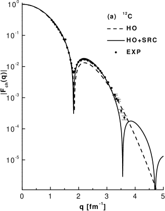
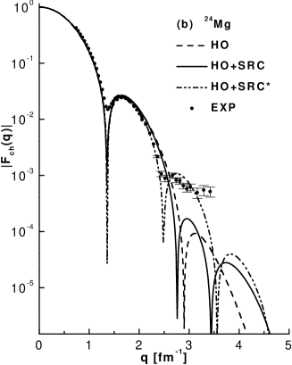
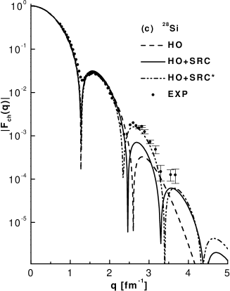
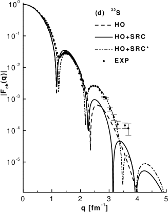
FIG. 1.: The charge form factor of the nuclei: ¹²C (a), ²⁴Mg (b), ²⁸Si (c) and ³²S (d) for various cases. Case HO+SRC* corresponds to the case when the occupation probability $\eta_{2s}$ is treated as a free parameter. The experimental points of ¹²C are from Ref. [42] and for the other nuclei from Ref. [43].

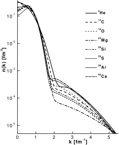
FIG. 2.: The correlated momentum distribution for various $s$-$p$ and $s$-$d$ shell nuclei calculated with the parameters $b$ and $\beta$ of case 2 when the nuclei ²⁴Mg, ²⁸Si, ³²S and ³⁶Ar were treated as $1d$ shell nuclei. The normalization is $\int n({\bf k}){\rm d}{\bf k}=1$.

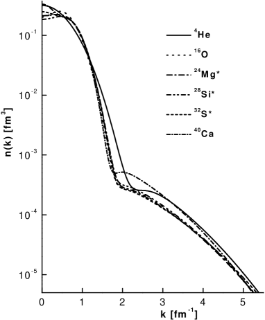
FIG. 3.: The correlated momentum distribution for the closed shell nuclei ⁴He, ¹⁶O, ⁴⁰Ca calculated as in Fig. 2 and for the open shell nuclei ²⁴Mg, ²⁸Si, ³²S calculated with the parameters $b$, $\beta$ and $\eta_{2s}$ of case 2* when they were treated as $1d$-$2s$ shell nuclei. The normalization is as in Fig. 2.

REFERENCES

• [1] M.L. Ristig, in From Nuclei to Particles, Proceedings of the International School of Physics ”Enrico Fermi,” Course LXXIX, Varenna, 1980, edited by A. Molinari (North-Holland, Amsterdam, 1982), p. 340.
• [2] A.N. Antonov, P.E. Hodgson, and I.Zh. Petcov, Nucleon Momentum and Density Distribution in Nuclei (Clarendon Press, Oxford, 1988)
• [3] Momentum Distribution, edited by R.N. Silver and P.E. Sokol (Plenum Press, New York, 1989).
• [4] J. G. Zabolitzky and W. Ey, Phys. Lett. 76B, 527 (1978).
• [5] A.N. Antonov, V.A. Nikolaev, and I.Zh. Petkov, Boulgarian Journal of Physics 6, 151 (1979); A.N. Antonov, V.A. Nikolaev, and I.Zh. Petkov, Z. Phys. A 297, 257 (1980); A.N. Antonov, C.V. Christov, and I.Zh. Petkov, Nuovo Cimento A 90 , 119 (1986); A.N. Antonov, I.S. Bonev, C.V. Christov, and I.Zh. Petkov, Nuovo Cimento A 100 , 779 (1988); A.N. Antonov, M.V. Stoitsov, L.P. Marinova, M.E. Grypeos, G.A. Lalazissis, and K.N. Ypsilantis, Phys. Rev. C 50, 1936 (1994).
• [6] O. Bohigas, and S. Stringari, Phys. Lett. 95B, 9 (1980).
• [7] M. Dal Ri, S. Stringari, and O. Bohigas, Nucl. Phys. A376, 81 (1982).
• [8] M.F. Flynn, J.W. Clark, R.M. Panoff, O. Bohigas, and S. Stringari, Nucl. Phys. A427, 253 (1984).
• [9] V.R. Pandharipande, C.N. Papanicolas, and J. Wambach, Phys. Rev. Lett. 53, 1133 (1984).
• [10] S. Fantoni and V. R. Pandharipande, Nucl. Phys. A427, 253 (1984).
• [11] M. Traini and G. Orlandini, Z. Phys. A 321, 479 (1985).
• [12] M. Jaminon, C. Mahaux, and H. NgΓ΄, Phys. Lett. 158B, 103 (1985); M. Jaminon, C. Mahaux, and H. NgΓ΄, Nucl.Phys. A440, 228 (1985); M. Jaminon, C. Mahaux, and H. NgΓ΄, Nucl.Phys. A452, 445 (1986).
• [13] O. Benhar, C.Ciofi degli Atti, S. Liuti, and G. SalmΓ¨, Phys. Lett. 177B, 135 (1986).
• [14] R. Schiavilla, V.R. Pandharipande, and R.B. Wiringa, Nucl.Phys. A449, 219 (1986).
• [15] M. Casas, J. Martorell, E. Moya de Guerra, and J. Treiner, Nucl. Phys. A473, 429 (1987).
• [16] S. Stringari, M. Traini, and O. Bohigas, Nucl. Phys. A516, 33 (1990).
• [17] M.V. Stoitsov, A.N. Antonov, and S.S. Dimitrova, Z. Phys. A 345, 359 (1993); M.V. Stoitsov, A.N.Antonov, and S.S. Dimitrova, Phys. Rev. C 47, 2455 (1993);
• [18] H. MΓΌther, A. Polls, and W.H. Dickhoff, Phys. Rev. C 51, 3040 (1995); H. MΓΌther, G. Knehr, and A. Polls, Phys. Rev. C 52, 2955 (1995);
• [19] M.K. Gaidarov, A.N.Antonov, G.S. Anagnostatos, S.E. Massen, M.V. Stoitsov, P.E. Hodgson, Phys. Rev C 52, 3026 (1995).
• [20] K.N.Ypsilantis and M.E. Grypeos, J. Phys. G 21, 1701 (1995); M.E. Grypeos and K.N. Ypsilantis, J. Phys. G 15, 1397 (1989).
• [21] A.N. Antonov, S.S. Dimitrova, M.K. Gaidarov, M.V. Stoitsov, M.E. Grypeos, S.E. Massen, and K.N. Ypsilantis, Nucl. Phys. A597, 163 (1996).
• [22] F. Arias de Saavedra, G. Co’, and M.M. Renis, Phys. Rev. C 55, 673 (1997).
• [23] G. Co’, A. Fabrocini, S. Fantoni, and I.E. Lagaris, Nucl. Phys. A549, 439 (1992); G. Co’, A. Fabrocini, S. Fantoni, Nucl. Phys. A568, 73 (1994); F. Arias de Saavedra, C. Co’, A. Fabrocini, and S. Fantoni, Nucl. Phys. A605, 359 (1996).
• [24] D.B. Day, J.S. McCarthy, Z.E. Meziani, R. Minehart, R. Sealock, S.T. Thornton, J. Jourdan, I. Sick, B.W. Filippone, R.D. McKeeown, R.G. Milner, D.H. Potterveld, and Z. Szalata, Phys. Rev. Lett. 59, 427 (1987).
• [25] X. Ji and R.D. McKeown, Phys. Lett. 236B, 130 (1990).
• [26] C. Ciofi degli Atti, E. Pace, and G. SalmΓ¨, Nucl. Phys. A497, 361c (1989).
• [27] C. Ciofi degli Atti, E. Pace, and G. SalmΓ¨, Phys. Rev. C 43, 1155 (1991).
• [28] M. Gaudin, J. Gillespie, and G. Ripka, Nucl. Phys. A176, 237 (1971).
• [29] F. Dellagiacoma, G. Orlandini, and M. Traini, Nucl. Phys. A393, 95 (1983).
• [30] E.N.M. Quint et al, Phys.Rev.Lett. 58, 1088 (1987).
• [31] S.E. Massen and Ch.C. Moustakidis, Phys. Rev. C 60, 024005 (1999).
• [32] M.K. Gaidarov, K.A. Pavlova, S.S. Dimitrova, M.V. Stoitsov, A.N. Antonov, D. Van Neck, and H. MΓΌther, Phys. Rev C 60, 024312 (1999).
• [33] P.A.M. Dirac : Proceedings of Cambridge Philosphpical Society 26, 376 (1930).
• [34] P.O. Lowdin, Phys. Rev. 97, 1474 (1955).
• [35] J.W. Clark, and M. L. Ristig, Nuov. Cim. LXXA 3, 313 (1970).
• [36] M.L. Ristig, W.J. Ter Low, and J.W. Clark, Phys. Rev. C 3, 1504 (1971).
• [37] J.W. Clark, Prog. Part. Nucl. Phys. 2, 89 (1979).
• [38] D.M. Brink and M.E. Grypeos, Nucl. Phys. A97, 81 (1967).
• [39] R. Jastrow, Phys. Rev. 98, 1497 (1955).
• [40] C. Ciofi degli Atti, E. Pace, and G. SalmΓ¨, Phys. Lett. 141B, 14 (1984).
• [41] H. De Vries, C.W. De Jager, and C. De Vries, Atom. Data and Nucl. Data Tables, 36, 495 (1987).
• [42] I. Sick, and J.S. McCarthy, Nucl.Phys. A150, 631 (1970).
• [43] G.C. Li, M.R. Yearian, and I. Sick, Phys. Rev. C 9, 1861 (1974).