Pertinent Dirac structure for QCD sum rules of meson-baryon coupling constants

Takumi Doi1 ***E-mail : doi@th.phys.titech.ac.jp    Hungchong Kim2 and Makoto Oka1 1 Department of Physics, Tokyo Institute of Technology, Tokyo 152-8551, Japan 2 Institute of Physics and Applied Physics, Yonsei University, Seoul 120-749, Korea
Abstract

Using general baryon interpolating fields $J_{B}$ for $B=N,\Xi,\Sigma,$ without derivative, we study QCD sum rules for meson-baryon couplings and their dependence on Dirac structures for the two-point correlation function with a meson $i\int d^{4}xe^{iqx}\langle 0|{\rm T}[J_{B}(x)\bar{J}_{B}(0)]|{\cal M}(p)\rangle$. Three distinct Dirac structures are compared: $i\gamma_{5}$, $i\gamma_{5}\ooalign{\hfil/\hfil\crcr$p$}$, and $\gamma_{5}\sigma_{\mu\nu}q^{\mu}p^{\nu}$ structures. From the dependence of the OPE on general baryon interpolating fields, we propose criteria for choosing an appropriate Dirac structure for the coupling sum rules. The $\gamma_{5}\sigma_{\mu\nu}q^{\mu}p^{\nu}$ sum rules satisfy the criteria while the $i\gamma_{5}$ sum rules beyond the chiral limit do not. For the $i\gamma_{5}\ooalign{\hfil/\hfil\crcr$p$}$ sum rules, the large continuum contributions prohibit reliable prediction for the couplings. Thus, the $\gamma_{5}\sigma_{\mu\nu}q^{\mu}p^{\nu}$ structure seems pertinent for realistic predictions. In the SU(3) limit, we identify the OPE terms responsible for the $F/D$ ratio. We then study the dependence of the ratio on the baryon interpolating fields. We conclude the ratio $F/D\sim 0.6-0.8$ for appropriate choice of the interpolating fields.

pacs:
PACS: 13.75.Gx; 12.38.Lg; 11.55.Hx
Keywords: QCD Sum rules; meson-baryon couplings, SU(3),$F/D$ ratio
††preprint: TIT/HEP-447/NP

I INTRODUCTION

In QCD sum rule approachesΒ [1], the two-point correlation function with a pion

$\displaystyle i\int d^{4}xe^{iq\cdot x}\langle 0|{\rm T}[J_{N}(x)\bar{J}_{N}(0)]|\pi(p)\rangle$ (1)

is often used to calculate the $\pi NN$ couplingΒ [2, 3, 4, 5, 6, 7, 8] by facilitating a general external field method developed in Ref.Β [9]. This correlation function contains three distinct Dirac structures (1) $i\gamma_{5}$ (PS), (2) $\gamma_{5}\sigma_{\mu\nu}q^{\mu}p^{\nu}$ (T), and (3) $i\gamma_{5}\ooalign{\hfil/\hfil\crcr$p$}$ (PV), each of which can in principle be used to calculate the coupling. Currently, there is an issue of the Dirac structure dependence of the sum rule resultsΒ [4, 5]. In calculating the coupling, one can construct either the PS sum rules beyond the chiral limitΒ [6, 7] or the T sum rulesΒ [4, 8]. Both sum rules yield the $\pi NN$ coupling close to its empirical value. On the other hand, the $i\gamma_{5}\ooalign{\hfil/\hfil\crcr$p$}$ sum rules contain large contributions from the continuum, which therefore do not provide reliable results.

The PS and T sum rules have been extended to calculate the meson-baryon couplings $\eta NN$, $\pi\Xi\Xi$, $\eta\Xi\Xi$, $\pi\Sigma\Sigma$ and $\eta\Sigma\Sigma$Β [7, 8] by considering the two-point correlation function with a meson,

$\displaystyle i\int d^{4}x~{}e^{iq\cdot x}\langle 0|{\rm T}[J_{B}(x)\bar{J}_{B}(0)]|{\cal M}(p)\rangle\ .$ (2)

Calculation of the couplings from this correlation function is somewhat limited due to the ignorance of meson wave functions when heavier mesons are involved. In the SU(3) limit however, this correlation function can be used to determine the so-called $F/D$ ratio unambiguously because in this limit the OPE can be exactly classified [7, 8] according to SU(3) relations for the couplings [10]. The $F/D$ ratio is an important input in making realistic potential models for hyperon-baryon interactions [11, 12] as well as in analyzing the hyperon semileptonic data.

At present, there is a clear Dirac structure dependence in the calculation of the $F/D$ ratio using Eq.Β (2). In particular, we have reported from the PS sum rules $F/D\sim 0.2$Β [7] while from T sum rules $F/D\sim 0.78$Β [8]. Thus, even though the two sum rules with different Dirac structures were successful in reproducing the empirical $\pi NN$ coupling, their prediction for the $F/D$ ratio is quite different.

To resolve this issue, additional criteria to choose a proper Dirac structure are needed for reliable predictions on the $F/D$ ratio as well as the meson-baryon couplings. For this purpose, we first note that in Ref.Β [7, 8] the Ioffe current or its SU(3) rotated version has been used to construct sum rules Eq.Β (2). The Ioffe current however is a specific choice for the nucleon current among infinitely many possibilities. The Ioffe current is often used for the nucleon because it gets large contributions from the chiral breaking parameter $\langle\bar{q}q\rangle$. In addition, direct instantons are believed to play less roles in this current.

Nevertheless, it may be useful to study the dependence of the sum rule results on general baryon currents. Depending on the currents, it is expected that the overlap $\lambda_{B}$ between the physical baryon state and the current may be altered but ideally the physical parameters such as meson-baryon couplings remain unchanged. Indeed, from the correlation function Eq.Β (2), what will actually be determined is the overlap strength multiplied by the coupling of concern. In the SU(3) symmetric limit, all the strengths depend only on the currents. They are determined from the corresponding baryon mass sum rules and all the baryon masses are the same in the SU(3) limit. Thus, in this limit, the dependence on the currents should be driven by the common overlap strength, which in return provides the coupling independent of the currents. This ideal aspect will be pursued in this work as a criterion for choosing a proper Dirac structure.

An alternative way is to calculate baryon axial charges and convert them into meson-baryon couplings using the Goldberger-Treiman relation. Ref.Β [13] considered the nucleon correlation function in external axial vector field and constructed a sum rule for $g_{A}-1$ using one specific Dirac structure. Recently, a new approach was proposed in Ref.Β [14] where the axial vector correlation function in a one-nucleon state is considered. Both obtained an excellent agreement for $g_{A}$ of the nucleon.

This paper is organized as follows. In SectionΒ II, we construct meson-baryon coupling sum rules using general baryon currents. A brief discussion on the OPE based on chirality is given in SectionΒ III. We then briefly check in SectionΒ IV whether the discussion on the continuum thresholdΒ [5, 8] is still valid when the general baryon currents are used in the sum rules. In SectionΒ V, the dependence of the OPE on the baryon currents is studied. We study in the SU(3) limit whether or not the dependence on the currents are mostly contained in the overlap $\lambda_{B}$. This constraint gives us a new criterion to choose an appropriate Dirac structure. In SectionΒ VI, we calculate the couplings in the SU(3) limit from the $\gamma_{5}\sigma_{\mu\nu}q^{\mu}p^{\nu}$ structure. The $F/D$ ratio is identified in terms of the OPE. Conclusions are given in SectionΒ VII.

II CONSTRUCTION of the QCD SUM RULES

We use the two-point correlation function with a meson,

$\displaystyle i\int d^{4}xe^{iq\cdot x}\langle 0|{\rm T}[J_{B}(x)\bar{J}_{B}(0)]|{\cal M}(p)\rangle$ (3)

where $J_{B}$ is the baryon current of concern and $p$ is the momentum of meson ${\cal M}$. Meson states $\pi$ and $\eta$, and baryon currents for the proton, $\Xi$ and $\Sigma$ will be considered in this work.

The proton current is constructed from two $u$-quarks and one $d$-quark by assuming that all three quarks are in the s-wave state. In the construction of the current, one up and one down quark are combined into an isoscalar diquark. The other up quark is attached to the diquark so that quantum numbers of the proton are carried by the attached up quark. In this method, there are two possible combinations for the current. The general proton current is a linear combination of the two possibilities mediated by a real parameter $t$,

$\displaystyle J_{p}(x;t)$ $\displaystyle=$ $\displaystyle 2\epsilon_{abc}[\ (u_{a}^{T}(x)Cd_{b}(x))\gamma_{5}u_{c}(x)+t\ (u_{a}^{T}(x)C\gamma_{5}d_{b}(x))u_{c}(x)\ ]\ .$ (4)

Here, $a,b,c$ are color indices, $T$ denotes the transpose with respect to the Dirac indices, and $C$ the charge conjugation. The choice $t=-1$ is called the Ioffe currentΒ [15]. The currents for $\Xi$ and $\Sigma$ are obtained from the proton current via SU(3) rotationsΒ [16],

$\displaystyle J_{\Xi}(x;t)$ $\displaystyle=$ βˆ’2​ϡa​b​c​[(saT​(x)​C​ub​(x))​γ5​sc​(x)+t​(saT​(x)​C​γ5​ub​(x))​sc​(x)],2subscriptitalic-Ο΅π‘Žπ‘π‘delimited-[]superscriptsubscriptπ‘ π‘Žπ‘‡π‘₯𝐢subscript𝑒𝑏π‘₯subscript𝛾5subscript𝑠𝑐π‘₯𝑑superscriptsubscriptπ‘ π‘Žπ‘‡π‘₯𝐢subscript𝛾5subscript𝑒𝑏π‘₯subscript𝑠𝑐π‘₯\displaystyle-2\epsilon_{abc}[\ (s_{a}^{T}(x)Cu_{b}(x))\gamma_{5}s_{c}(x)+t\ (s_{a}^{T}(x)C\gamma_{5}u_{b}(x))s_{c}(x)\ ]\ , (5)
$\displaystyle J_{\Sigma}(x;t)$ $\displaystyle=$ $\displaystyle\ \ 2\epsilon_{abc}[\ (u_{a}^{T}(x)Cs_{b}(x))\gamma_{5}u_{c}(x)+t\ (u_{a}^{T}(x)C\gamma_{5}s_{b}(x))u_{c}(x)\ ]\ .$ (6)

When going beyond the soft-meson limit, one can consider three distinct Dirac structures in correlation function in constructing sum rules: $i\gamma_{5}$ (PS), $\gamma_{5}\sigma_{\mu\nu}q^{\mu}p^{\nu}$ (T) and $i\gamma_{5}\ooalign{\hfil/\hfil\crcr$p$}$ (PV). For the $i\gamma_{5}$ structure, the sum rules are constructed at the order $p^{2}=m_{\pi}^{2}$ Β [6]. At this order, the terms linear in quark mass $(m_{q})$ in the OPE should be included because $m_{q}$ is the same chiral order with $m_{\pi}^{2}$ via the Gell-Mann–Oakes–Renner relation,

$\displaystyle-2m_{q}\langle\bar{q}q\rangle=m_{\pi}^{2}f_{\pi}^{2}\ .$ (7)

On the other hand, for the T and PV structures, we construct the sum rules at the order ${\cal O}(p)$. At this order, the $m_{q}$ terms should not be included in the OPE. Technical details on the OPE calculation can be found in Refs.Β [7, 8].

In constructing the phenomenological side, we first define $\lambda_{B}(t)$, the coupling strength between the baryon current $J_{B}(x;t)$ and the physical baryon field $\psi_{B}(x)$. Using the pseudoscalar type interaction between the meson and baryons $g_{{\cal M}B}\bar{\psi}_{B}i\gamma_{5}\psi_{B}{\cal M}$, we obtain the phenomenological side of the correlation function:

$\displaystyle i\gamma_{5}\ \mbox{structure}$ $\displaystyle\ \mbox{at the order}\ {\cal O}(p^{2})\qquad i\gamma_{5}p^{2}\frac{g_{{\cal M}B}\lambda_{B}^{2}(t)}{(q^{2}-m_{B}^{2})^{2}}+\cdots\ ,$ (8)
$\displaystyle\gamma_{5}\sigma_{\mu\nu}q^{\mu}p^{\nu}\ \mbox{structure}$ $\displaystyle\ \mbox{at the order}\ {\cal O}(p)\qquad\gamma_{5}\sigma_{\mu\nu}q^{\mu}p^{\nu}\frac{g_{{\cal M}B}\lambda_{B}^{2}(t)}{(q^{2}-m_{B}^{2})^{2}}+\cdots\ ,$ (9)
$\displaystyle i\gamma_{5}\ooalign{\hfil/\hfil\crcr$p$}\ \mbox{structure}$ $\displaystyle\ \mbox{at the order}\ {\cal O}(p)\qquad-i\gamma_{5}\ooalign{\hfil/\hfil\crcr$p$}\frac{g_{{\cal M}B}\lambda_{B}^{2}(t)m_{B}}{(q^{2}-m_{B}^{2})^{2}}+\cdots\ .$ (14)

The ellipsis denotes contributions from higher resonances as well as a single pole associated with transitions from the ground state to higher resonances. The continuum contributions come from transitions among higher resonances, whose spectral densities are modeled with a step function starting at the threshold $S_{0}$. Matching the OPE side with the phenomenological side and taking Borel transformation †††Note, we use a single dispersion relation as advocated in Ref.Β [17, 18]., we get the sum rules of the form

$\displaystyle g_{{\cal M}B}\lambda_{B}^{2}(t)\left[\ 1+A_{{\cal M}B}(t)M^{2}\ \right]$ $\displaystyle=$ $\displaystyle e^{m_{B}^{2}/M^{2}}\cdot F^{\mbox{OPE}}_{\mbox{\it${\cal M}$B}}(M^{2};t)\quad\equiv\quad f^{\mbox{OPE}}_{\mbox{\it${\cal M}$B}}(M^{2};t)$ (15)

where the single pole term in the phenomenological side has been denoted by $A_{{\cal M}B}$. Expressions for the OPE $F^{\mbox{OPE}}_{\mbox{\it${\cal M}$B}}(M^{2};t)$ are given in the AppendixΒ A.

III Chirality consideration

The OPEs given in the AppendixΒ A have an interesting feature to discuss when $t=1$. Specifically, in the $i\gamma_{5}$ and $\gamma_{5}\sigma_{\mu\nu}q^{\mu}p^{\mu}$ sum rules, Wilson coefficients of chiral-odd operators $\langle\bar{q}q\rangle$, $f_{3\pi}$, ⟨q¯​qβŸ©β€‹βŸ¨Ξ±sπ​𝒒2⟩delimited-βŸ¨βŸ©Β―π‘žπ‘ždelimited-⟨⟩subscriptπ›Όπ‘ πœ‹superscript𝒒2\langle\bar{q}q\rangle\left\langle{\alpha_{s}\over\pi}{\cal G}^{2}\right\rangle, and $m_{0}^{2}\langle\bar{q}q\rangle$ are all zero when $t=1$. Also in the $i\gamma_{5}\ooalign{\hfil/\hfil\crcr$p$}$ sum rules, contributions from the chiral-even operators $\langle\bar{q}q\rangle^{2}$ and $m_{0}^{2}\langle\bar{q}q\rangle^{2}$ are zero. To understand this feature, it is useful to decompose the correlator according to chirality of the current,

$\displaystyle J_{B}\bar{J}_{B}=J^{R}_{B}\bar{J}^{R}_{B}+J^{R}_{B}\bar{J}^{L}_{B}+J^{L}_{B}\bar{J}^{R}_{B}+J^{L}_{B}\bar{J}^{L}_{B}\ .$ (16)

$J^{L}_{B}(J^{R}_{B})$ denotes the left-handed (right-handed) component of the current $J_{B}$. On the other hand, Eq.Β (3) can be written

iβ€‹βˆ«d4​x​ei​qβ‹…xβ€‹βŸ¨0|T​[JB​(x)​JΒ―B​(0)]|ℳ​(p)βŸ©π‘–superscript𝑑4π‘₯superscriptπ‘’β‹…π‘–π‘žπ‘₯quantum-operator-product0Tdelimited-[]subscript𝐽𝐡π‘₯subscript¯𝐽𝐡0ℳ𝑝\displaystyle i\int d^{4}xe^{iq\cdot x}\langle 0|{\rm T}[J_{B}(x)\bar{J}_{B}(0)]|{\cal M}(p)\rangle =\displaystyle= i​γ5​Πps+i​γ5​/p​Πpv𝑖subscript𝛾5subscriptΞ ps𝑖subscript𝛾5/𝑝subscriptΞ pv\displaystyle i\gamma_{5}~{}\Pi_{\rm ps}+i\gamma_{5}\ooalign{\hfil/\hfil\crcr$p$}~{}\Pi_{\rm pv} (19)
$\displaystyle+$ Ξ³5​σμ​ν​qμ​pν​ΠT.subscript𝛾5subscriptπœŽπœ‡πœˆsuperscriptπ‘žπœ‡superscriptπ‘πœˆsubscriptΞ T\displaystyle\gamma_{5}\sigma_{\mu\nu}q^{\mu}p^{\nu}~{}\Pi_{\rm T}\ . (20)

Thus, it is easy to see that the $i\gamma_{5}$ and $\gamma_{5}\sigma_{\mu\nu}$ structures have nonzero contributions only from the chiral mixing term $J^{R}\bar{J}^{L}+J^{L}\bar{J}^{R}$, while the chirality conserving term $J^{R}\bar{J}^{R}+J^{L}\bar{J}^{L}$ contributes only to the $i\gamma_{5}\ooalign{\hfil/\hfil\crcr$p$}$ structure.

Now let us classify QCD operators contributing to each Dirac structure. To do that, we suppress for simplicity the color indices and write baryon current as

$$J\sim(q^{T}Cq)\gamma_{5}q+t\ (q^{T}C\gamma_{5}q)q\ .$$ (21)

Here q=u,d,sπ‘žπ‘’π‘‘π‘ q=u,d,s. When $t=1$, it is straightforward to show that

$\displaystyle J_{R}$ $\displaystyle\sim$ $\displaystyle 2(q_{R}^{T}Cq_{R})q_{R}\ ,$ (22)
$\displaystyle J_{L}$ $\displaystyle\sim$ $\displaystyle-2(q_{L}^{T}Cq_{L})q_{L}\ .$ (23)

Thus, at this specific $t$, chirality of all quarks are the same as that of the baryon.

In the $i\gamma_{5}$ or $\gamma_{5}\sigma_{\mu\nu}$ sum rules, we need to consider the products $J^{R}\bar{J}^{L}$ and $J^{L}\bar{J}^{R}$. In making such products using Eqs.Β (22) (23), all three quark propagators should break the chirality when they move from the coordinate 00 to $x$. Hence, it is easy to see that, among chiral-odd operators, terms such as

$$m_{q}\langle\bar{q}q\rangle^{2},\langle\bar{q}q\rangle^{3},m_{q}^{2}\langle\bar{q}q\rangle,\cdots$$ (24)

can contribute to the $i\gamma_{5}$ or $\gamma_{5}\sigma_{\mu\nu}$ correlator, while other chiral-odd operators such as $\langle\bar{q}q\rangle$, $f_{3\pi}$, ⟨q¯​qβŸ©β€‹βŸ¨Ξ±sπ​𝒒2⟩delimited-βŸ¨βŸ©Β―π‘žπ‘ždelimited-⟨⟩subscriptπ›Όπ‘ πœ‹superscript𝒒2\langle\bar{q}q\rangle\left\langle{\alpha_{s}\over\pi}{\cal G}^{2}\right\rangle, $m_{0}^{2}\langle\bar{q}q\rangle$ cannot.

On the other hand, in the $i\gamma_{5}\ooalign{\hfil/\hfil\crcr$p$}$ structure, the product $J^{L}\bar{J}^{L}$ or $J^{R}\bar{J}^{R}$ contributes to the sum rule. Among chiral-even operators, an operator such as $\langle\bar{q}q\rangle^{2}$ cannot be formed in the product $J^{L}\bar{J}^{L}$ or $J^{R}\bar{J}^{R}$ simply because two quarks with the same chirality cannot be combined into the quark-antiquark pair. Similarly, $m_{0}^{2}\langle\bar{q}q\rangle^{2}$ can not be formed. This explains the disappearance of such terms in the OPE when $t=1$.

IV Criterion I : sensitivity to the continuum threshold

We now analyze sum rules of the three different Dirac structures with the general baryon currents, EqsΒ (4) and (6). As pointed out in Refs.Β [5, 8], sum rule results from the $i\gamma_{5}\ooalign{\hfil/\hfil\crcr$p$}$ structure are sensitive to the continuum threshold $S_{0}$ and therefore this structure is not reliable. On the other hand, $i\gamma_{5}$ and $\gamma_{5}\sigma_{\mu\nu}q^{\mu}p^{\nu}$ structures are insensitive to $S_{0}$. The chirality consideration suggested in Ref.Β [5] implies that in the $i\gamma_{5}\ooalign{\hfil/\hfil\crcr$p$}$ sum rules the large slope and the strong sensitivity to $S_{0}$ of the Borel curves can be explained if higher resonances with different parities add up. With this scenario, the higher resonances contributions cancel each other in the $i\gamma_{5}$ and $\gamma_{5}\sigma_{\mu\nu}q^{\mu}p^{\nu}$ sum rules therefore explaining the weak sensitivity to $S_{0}$ and the small slope of the Borel curves.

Since only the Ioffe current is used in the analysis of Refs.Β [5, 8], let us briefly check if this scenario still works when the general baryon currents are used. As the scenario does not rely on the specific form for the current, what has been claimed in Refs.Β [5, 8] must be valid even with the general baryon currents.
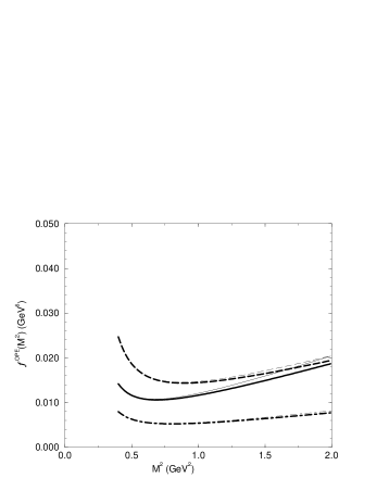
 To see this, we plot the RHS of Eq.Β (15) for the π​N​Nπœ‹π‘π‘\pi NN coupling from i​γ5𝑖subscript𝛾5i\gamma_{5}, Ξ³5​σμ​ν​qμ​pΞ½subscript𝛾5subscriptπœŽπœ‡πœˆsuperscriptπ‘žπœ‡superscriptπ‘πœˆ\gamma_{5}\sigma_{\mu\nu}q^{\mu}p^{\nu} and i​γ5​/p𝑖subscript𝛾5/𝑝i\gamma_{5}\ooalign{\hfil/\hfil\crcr$p$} structures in Figs.Β 1,Β 2,Β 3, respectively. To show the dependence on t𝑑t, we plot the curves for t=βˆ’1.5,1.5𝑑1.51.5t=-1.5,1.5 as well as t=βˆ’1.0𝑑1.0t=-1.0 (the Ioffe current). In these plots, we use the standard QCD parameters,

$\displaystyle\langle\bar{q}q\rangle$ $\displaystyle=$ βˆ’(0.23​GeV)3;⟨αsπ​𝒒2⟩=(0.33​GeV)4,superscript0.23GeV3delimited-⟨⟩subscriptπ›Όπ‘ πœ‹superscript𝒒2superscript0.33GeV4\displaystyle-(0.23~{}{\rm GeV})^{3}\;;\quad\left\langle{\alpha_{s}\over\pi}{\cal G}^{2}\right\rangle=(0.33~{}{\rm GeV})^{4}\ , (25)
$\displaystyle\delta^{2}$ $\displaystyle=$ $\displaystyle 0.2~{}{\rm GeV}^{2}\;;\quad m_{0}^{2}=0.8~{}{\rm GeV}^{2}\ .$ (26)

For each $t$, the thick lines are for the continuum threshold $S_{0}=2.07\ {\rm GeV}^{2}$ corresponding to the Roper resonance, while the thin lines for $S_{0}=2.57\ {\rm GeV}^{2}$. The trend observed here is the same for the other couplings.

In Fig.Β 3, we observe that the $i\gamma_{5}\ooalign{\hfil/\hfil\crcr$p$}$ structure is sensitive to the continuum threshold even when the general current is used. The difference by changing the continuum threshold is $\sim 15\%$ at $M^{2}=1~{}{\rm GeV}^{2}$. Note also that the slope is relatively large in this case. Since the coupling is determined from the intersection of the best fitting curve with the vertical line at $M^{2}=0$ (see Eq.Β (15)), the $15\%$ change at $M^{2}=1~{}{\rm GeV}^{2}$, when it combined with the large slope, produces huge change in the extracted coupling. In contrast, from Figs.Β 1 and Β 2, the $i\gamma_{5}$ and $\gamma_{5}\sigma_{\mu\nu}q^{\mu}p^{\nu}$ structures are insensitive to $S_{0}$. Also the slopes of the curves are small. This observation is practically independent of the parameter $t$. At $M^{2}=1~{}{\rm GeV}^{2}$, the difference is only $2-3\%$ level. Thus, the analysis in Refs.Β [5, 8] is still valid and the sum rule results from $i\gamma_{5}\ooalign{\hfil/\hfil\crcr$p$}$ structure should be discarded under this consideration.

V Criterion II : the dependence of the OPE on baryon currents

Using the sum rules derived in SectionΒ II, we discuss the dependence of the OPE on the baryon current (i.e. the dependence on $t$). For a given $t$, we linearly fit the RHS of Eq.Β (15)

$\displaystyle g_{{\cal M}B}\lambda_{B}^{2}(t)\left[\ 1+A_{{\cal M}B}(t)M^{2}\ \right]\ =\ f^{\mbox{OPE}}_{\mbox{\it${\cal M}$B}}(M^{2};t)\ ,$

and determine $\left[g_{{\cal M}B}\lambda_{B}^{2}(t)\right]_{\mbox{fitted}}$. Because $f^{\mbox{OPE}}_{\mbox{\it${\cal M}$B}}$ is quadratic in $t$, $\left[g_{{\cal M}B}\lambda_{B}^{2}(t)\right]_{\mbox{fitted}}$ is also quadratic. Ideally, the physical parameter $g_{{\cal M}B}$ should be independent of $t$ if the sum rules are reliable. In other words, $t$ is just a parameter for the current. By changing $t$, only the coupling strength $\lambda_{B}^{2}(t)$ is expected to be affected, but not the physical parameter. This is a constraint to be satisfied when the sum rules are β€œgood.”

To proceed, we take the SU(3) symmetric limit. Then, the strength $\lambda_{B}(t)$ should be independent of the baryons,

$\displaystyle\lambda_{N}(t)=\lambda_{\Xi}(t)=\lambda_{\Sigma}(t)\ ,$ (27)

as the baryon mass sum rules are the same in the limit. Furthermore, we have

⟨s¯​s⟩=⟨q¯​q⟩delimited-βŸ¨βŸ©Β―π‘ π‘ delimited-βŸ¨βŸ©Β―π‘žπ‘ž\displaystyle\langle\bar{s}s\rangle=\langle\bar{q}q\rangle $\displaystyle\;;\quad m_{\eta}=m_{\pi}\ ,$ (28)
$\displaystyle f_{\eta}=f_{\pi}$ $\displaystyle\;;\quad f_{3\eta}=f_{3\pi}\ ,$ (29)
$\displaystyle m_{N}=m_{\Xi}=m_{\Sigma}$ $\displaystyle\;;\quad m_{s}=m_{q}\ .$ (30)

This SU(3) limit is particularly interesting when we select a suitable Dirac structure. Suppose we plot $\left[g_{{\cal M}B}\lambda_{B}^{2}(t)\right]_{\mbox{fitted}}$ in terms of $t$. If the sum rules are β€œgood”, all $g_{{\cal M}B}$ should be just constants, independent of $t$. The functional behavior is driven only by the strength $\lambda_{B}^{2}(t)$. The baryon mass sum rules in the SU(3) limit constrain that all $\lambda_{B}^{2}(t)$ are the same irrespective of the baryons. Therefore, β€œgood” sum rules must give $\left[g_{{\cal M}B}\lambda_{B}^{2}(t)\right]_{\mbox{fitted}}$ which are proportional to each other.

Our constraint should be satisfied when the OPE are exact. But in practice, the full OPE terms $f^{\rm OPE}_{\rm full}$ are separated into two groups,

$\displaystyle f^{\rm OPE}_{\rm full}=f^{\rm OPE}_{\rm calc}+f^{\rm OPE}_{\rm rest}\ ,$ (31)

where $f^{\rm OPE}_{\rm calc}$ denotes the calculable OPE, and $f^{\rm OPE}_{\rm rest}$ denotes the rest of the full OPE. In this notation, the reliability of sum rule simply means

$\displaystyle f^{\rm OPE}_{\rm calc}\gg f^{\rm OPE}_{\rm rest}\ .$ (32)

The sum rules are β€œunreliable” if

$\displaystyle f^{\rm OPE}_{\rm calc}\sim f^{\rm OPE}_{\rm rest}\ .$ (33)

In the former case, we expect that $\left[g_{{\cal M}B}\lambda_{B}^{2}(t)\right]_{\mbox{fitted}}$ derived from $f^{\mbox{OPE}}_{\mbox{\it${\cal M}$B;\rm\ calc}}$ is almost the same as those from $f^{\mbox{OPE}}_{\mbox{\it${\cal M}$B;\rm\ full}}$ in most region of $t$. On the other hand, in the latter case, $\left[g_{{\cal M}B}\lambda_{B}^{2}(t)\right]_{\mbox{fitted}}$ derived from $f^{\mbox{OPE}}_{\mbox{\it${\cal M}$B;\rm\ calc}}$ may be quite different from those obtained from $f^{\mbox{OPE}}_{\mbox{\it${\cal M}$B;\rm\ full}}$, and our ideal constraint may not be satisfied in most $t$.

Therefore, the ideal constraint can be used as a new criterion for choosing reliable sum rules. In order to apply this constraint to our sum rules, we again use the standard QCD parameters Eq.Β (26) and linearly fit [gℳ​B​λB2​(t)]fittedsubscriptdelimited-[]subscript𝑔ℳ𝐡superscriptsubscriptπœ†π΅2𝑑fitted\left[g_{{\cal M}B}\lambda_{B}^{2}(t)\right]_{\mbox{fitted}} at each t𝑑t. In the fitting, the continuum threshold is set to S0=2.07​GeV2subscript𝑆02.07superscriptGeV2S_{0}=2.07\ {\rm GeV^{2}}, corresponding to the Roper resonance, and the Borel window is taken 0.65≀M2≀1.24​GeV20.65superscript𝑀21.24superscriptGeV20.65\leq M^{2}\leq 1.24\ {\rm GeV^{2}}\ as in Refs.Β [6, 7, 8]. In this Borel window, (1) the Borel curve for each coupling is almost linear (see Figs.Β 1,Β 2), (2) the contribution from the highest dimensional OPE term is typically 5βˆ’15%5percent155-15\% in the Ξ³5​σμ​ν​qμ​pΞ½subscript𝛾5subscriptπœŽπœ‡πœˆsuperscriptπ‘žπœ‡superscriptπ‘πœˆ\gamma_{5}\sigma_{\mu\nu}q^{\mu}p^{\nu} sum rules and 20%percent2020\% level in the i​γ5𝑖subscript𝛾5i\gamma_{5} sum rules, and (3) the continuum contribution is less than 20%percent2020\% in both structures. It should be noted that because all the couplings are related under SU(3) rotations, we need to take a common Borel windowΒ [7, 8].

Fig.Β 4 shows $\left[g_{{\cal M}B}\lambda_{B}^{2}(t)\right]_{\mbox{fitted}}$ as a function of $t$ for the $i\gamma_{5}$ sum rules. The $\gamma_{5}\sigma_{\mu\nu}q^{\mu}p^{\nu}$ cases are shown in Fig.Β 5. Interesting features in the $\gamma_{5}\sigma_{\mu\nu}q^{\mu}p^{\nu}$ cases are that (1) all the curves are zero when $t=1$ and almost zero at $t\sim-0.5$, (2) each extremum of the curves coincides around $t\sim 0.3$. Under the chirality consideration given in Section Β III, we can easily understand why $\left[g_{{\cal M}B}\lambda_{B}^{2}(t)\right]_{\mbox{fitted}}$ is zero when $t=1$. From the figure, though not exact, one observes that the curves can be almost overlapped when multiplied by appropriate constants. For example, let us compare the $\pi NN$ and $\eta NN$ curves. When they are positive, the $\pi NN$ curve lies above the $\eta NN$ curve. When they are negative, the situation is reversed. This behavior of the $\eta NN$ curve can be reproduced by multiplying an appropriate constant to the $\pi NN$ curve. Of course, this claim can not be made when $t\sim-0.5$ because one curve becomes zero while the other does not. Therefore, except around $t\sim-0.5$, the Borel curves satisfy the ideal constraint in most region of $t$. Such a trend can not be observed from the $i\gamma_{5}$ sum rules. (see Fig.Β 4.) Therefore, we claim that the $\gamma_{5}\sigma_{\mu\nu}q^{\mu}p^{\nu}$ sum rules are more appropriate.

To support our claim that the $\gamma_{5}\sigma_{\mu\nu}q^{\mu}p^{\nu}$ sum rules are more suitable than those from the $i\gamma_{5}$ structure, one more check to do is to see the $t$-dependence of $\lambda_{B}^{2}(t)$ from baryon mass sum rules. In Fig.Β 6, $\lambda_{B}^{2}(t)$ in the SU(3) limit is plotted using chiral-odd nucleon mass sum rule ‑‑‑Definition of the function $E_{n}(x\equiv S_{0}/M^{2})$ is given in the AppendixΒ A. The Wilson coefficient of the dimension 7 OPE is different from Ref.Β [19]. When $t=-1$ (the Ioffe current), however, our Wilson coefficient reduces to that of Ref.Β [9]. Nevertheless, the dimension 7 condensate contributes to the sum rule only slightly. Thus, this discrepancy is marginal.:

$\displaystyle m_{B}\lambda_{B}^{2}(t)e^{-m_{B}^{2}/M^{2}}$ $\displaystyle=$ $\displaystyle\frac{-4}{(2\pi)^{4}}\left[\ \frac{\pi^{2}}{4}(-5-2t+7t^{2})\langle\bar{q}q\rangle M^{4}E_{1}(x)\right.$ (36)
$\displaystyle+\frac{3}{4}\pi^{2}(1-t^{2})m_{0}^{2}\langle\bar{q}q\rangle M^{2}E_{0}(x)$
$\displaystyle\left.+\frac{\pi^{4}}{24}(-7+2t+5t^{2})\langle\bar{q}q\rangle\left\langle{\alpha_{s}\over\pi}{\cal G}^{2}\right\rangle\ \right]\ ,$

where $m_{q}$ order terms are neglected and the SU(3) relations are used: $m_{N}=m_{\Xi}=m_{\Sigma}\equiv m_{B}$; $\lambda_{N}=\lambda_{\Xi}=\lambda_{\Sigma}\equiv\lambda_{B}$; ⟨u¯​u⟩=⟨d¯​d⟩=⟨s¯​sβŸ©β‰‘βŸ¨q¯​q⟩delimited-βŸ¨βŸ©Β―π‘’π‘’delimited-βŸ¨βŸ©Β―π‘‘π‘‘delimited-βŸ¨βŸ©Β―π‘ π‘ delimited-βŸ¨βŸ©Β―π‘žπ‘ž\langle\bar{u}u\rangle=\langle\bar{d}d\rangle=\langle\bar{s}s\rangle\equiv\langle\bar{q}q\rangle. Comparing with Fig.Β 5, we confirm that the $t$-dependence of $\left[g_{{\cal M}B}\lambda_{B}^{2}(t)\right]_{\mbox{fitted}}$ from the $\gamma_{5}\sigma_{\mu\nu}q^{\mu}p^{\nu}$ sum rules can be reproduced from the $t$-dependence of $\lambda_{B}^{2}(t)$.

In the region βˆ’0.5<∼t<∼1fragmentsfragmentssimilar-to0.5𝑑fragmentsfragmentssimilar-to1-0.5\mathrel{\mathchoice{\lower 2.58334pt\vbox{\halign{$\m@th\displaystyle\hfill#\hfil$\cr<\crcr\sim\crcr}}}{\lower 2.58334pt\vbox{\halign{$\m@th\textstyle\hfill#\hfil$\cr<\crcr\sim\crcr}}}{\lower 2.58334pt\vbox{\halign{$\m@th\scriptstyle\hfill#\hfil$\cr<\crcr\sim\crcr}}}{\lower 2.58334pt\vbox{\halign{$\m@th\scriptscriptstyle\hfill#\hfil$\cr<\crcr\sim\crcr}}}}t\mathrel{\mathchoice{\lower 2.58334pt\vbox{\halign{$\m@th\displaystyle\hfill#\hfil$\cr<\crcr\sim\crcr}}}{\lower 2.58334pt\vbox{\halign{$\m@th\textstyle\hfill#\hfil$\cr<\crcr\sim\crcr}}}{\lower 2.58334pt\vbox{\halign{$\m@th\scriptstyle\hfill#\hfil$\cr<\crcr\sim\crcr}}}{\lower 2.58334pt\vbox{\halign{$\m@th\scriptscriptstyle\hfill#\hfil$\cr<\crcr\sim\crcr}}}}1 in Fig.Β 6, Ξ»B2​(t)superscriptsubscriptπœ†π΅2𝑑\lambda_{B}^{2}(t) is negative, thus not physical. In this region, the sum rules should definitely fail and a reliable prediction for a physical parameter may not be possible. At tβˆΌβˆ’0.5similar-to𝑑0.5t\sim-0.5 or t∼1similar-to𝑑1t\sim 1, of course, the OPE is almost zero suggesting that there are cancellations among OPE terms, i.e. the correlation function can not be well saturated by the calculated OPE. Therefore, the optimal current should be chosen away from these points.

VI The $F/D$ ratio from the pseudotensor sum rules

In this section, we analyze the $\gamma_{5}\sigma_{\mu\nu}q^{\mu}p^{\nu}$ sum rules to determine the $F/D$ ratio. In particular, we investigate the $t$-dependence of the ratio using the general interpolating fields for the baryons. As already mentioned, mesons and baryons are classified according to SU(3) symmetry, which provides simple relations for the meson-baryon couplings in terms of the two parametersΒ [10]

$$g_{\pi N}~{}~{}{\rm and}~{}~{}\alpha={F\over F+D}\ .$$ (37)

That is,

$\displaystyle g_{\eta N}$ $\displaystyle=$ $\displaystyle\frac{1}{\sqrt{3}}(4\alpha-1)g_{\pi N}\;;\quad g_{\pi\Xi}=(2\alpha-1)g_{\pi N}\ ,$ (38)
$\displaystyle g_{\eta\Xi}$ $\displaystyle=$ $\displaystyle-\frac{1}{\sqrt{3}}(1+2\alpha)g_{\pi N}\;;\quad g_{\pi\Sigma}=2\alpha\ g_{\pi N}\ ,$ (39)
$\displaystyle g_{\eta\Sigma}$ $\displaystyle=$ $\displaystyle\frac{2}{\sqrt{3}}(1-\alpha)g_{\pi N}\ .$ (40)

To see how these relations are reflected in the OPE of the $\gamma_{5}\sigma_{\mu\nu}q^{\mu}p^{\nu}$ sum rules (see the AppendixΒ A for the OPE), we take the SU(3) symmetric limit to organize them in terms of two terms ${\cal O}_{1}$ and ${\cal O}_{2}$ defined as

$\displaystyle{\cal O}_{1}\cdot e^{-m_{B}^{2}/M^{2}}\quad$ $\displaystyle\equiv\quad$ $\displaystyle\frac{1}{96\pi^{2}f_{\pi}}(-2+4t-2t^{2})\langle\bar{q}q\rangle M^{4}E_{0}(x)-\frac{f_{\pi}}{3}(-1+t^{2})\langle\bar{q}q\rangle M^{2}$ (43)
βˆ’154​fπ​δ2​7​(βˆ’1+t2)β€‹βŸ¨q¯​q⟩+172β‹…12​fπ​(βˆ’1+2​tβˆ’t2)β€‹βŸ¨q¯​qβŸ©β€‹βŸ¨Ξ±sπ​𝒒2⟩154subscriptπ‘“πœ‹superscript𝛿271superscript𝑑2delimited-βŸ¨βŸ©Β―π‘žπ‘ž1β‹…7212subscriptπ‘“πœ‹12𝑑superscript𝑑2delimited-βŸ¨βŸ©Β―π‘žπ‘ždelimited-⟨⟩subscriptπ›Όπ‘ πœ‹superscript𝒒2\displaystyle-\frac{1}{54}f_{\pi}\delta^{2}7(-1+t^{2})\langle\bar{q}q\rangle+\frac{1}{72\cdot 12f_{\pi}}(-1+2t-t^{2})\langle\bar{q}q\rangle\left\langle{\alpha_{s}\over\pi}{\cal G}^{2}\right\rangle
$\displaystyle+\frac{f_{\pi}}{72}7(-1+t^{2})m_{0}^{2}\langle\bar{q}q\rangle\ ,$
$\displaystyle{\cal O}_{2}\cdot e^{-m_{B}^{2}/M^{2}}\quad$ $\displaystyle\equiv\quad$ $\displaystyle\frac{1}{96\pi^{2}f_{\pi}}12(1-t^{2})\langle\bar{q}q\rangle M^{4}E_{0}(x)+\frac{2f_{\pi}}{3}(t-t^{2})\langle\bar{q}q\rangle M^{2}$ (46)
βˆ’127​fπ​δ2​(3βˆ’13​t+10​t2)β€‹βŸ¨q¯​q⟩+148​fπ​(1βˆ’t2)β€‹βŸ¨q¯​qβŸ©β€‹βŸ¨Ξ±sπ​𝒒2⟩127subscriptπ‘“πœ‹superscript𝛿2313𝑑10superscript𝑑2delimited-βŸ¨βŸ©Β―π‘žπ‘ž148subscriptπ‘“πœ‹1superscript𝑑2delimited-βŸ¨βŸ©Β―π‘žπ‘ždelimited-⟨⟩subscriptπ›Όπ‘ πœ‹superscript𝒒2\displaystyle-\frac{1}{27}f_{\pi}\delta^{2}(3-13t+10t^{2})\langle\bar{q}q\rangle+\frac{1}{48f_{\pi}}(1-t^{2})\langle\bar{q}q\rangle\left\langle{\alpha_{s}\over\pi}{\cal G}^{2}\right\rangle
$\displaystyle+\frac{f_{\pi}}{36}(1-3t+2t^{2})m_{0}^{2}\langle\bar{q}q\rangle\ .$

Specifically, we have

$\displaystyle g_{\pi N}\cdot\lambda_{N}^{2}(1+A_{\pi N}M^{2})=$ $\displaystyle{\cal O}_{1}$ $\displaystyle+{\cal O}_{2}\ ,$ (47)
$\displaystyle\sqrt{3}g_{\eta N}\cdot\lambda_{N}^{2}(1+A_{\eta N}M^{2})=$ $\displaystyle-{\cal O}_{1}$ $\displaystyle+{\cal O}_{2}\ ,$ (48)
$\displaystyle g_{\pi\Xi}\cdot\lambda_{N}^{2}(1+A_{\pi\Xi}M^{2})=$ $\displaystyle-{\cal O}_{1}$ $\displaystyle\ ,$ (49)
$\displaystyle\sqrt{3}g_{\eta\Xi}\cdot\lambda_{N}^{2}(1+A_{\eta\Xi}M^{2})=$ $\displaystyle-{\cal O}_{1}$ $\displaystyle-2{\cal O}_{2}\ ,$ (50)
$\displaystyle g_{\pi\Sigma}\cdot\lambda_{N}^{2}(1+A_{\pi\Sigma}M^{2})=$ $\displaystyle\ \ {\cal O}_{2}\ ,$ (51)
$\displaystyle\sqrt{3}g_{\eta\Sigma}\cdot\lambda_{N}^{2}(1+A_{\eta\Sigma}M^{2})=$ $\displaystyle 2{\cal O}_{1}$ $\displaystyle+{\cal O}_{2}\ .$ (52)

Note that another SU(3) relation $\lambda_{N}=\lambda_{\Xi}=\lambda_{\Sigma}$ has been used in writing these equations. Neglecting the unknown single pole term $A_{{\cal M}B}$, we identify the $F/D$ ratio in terms of the OPE,

$\displaystyle 2\alpha\sim\frac{{\cal O}_{2}}{{\cal O}_{1}+{\cal O}_{2}}\quad\longrightarrow\quad F/D\sim\frac{{\cal O}_{2}}{2{\cal O}_{1}+{\cal O}_{2}}\ .$ (53)

This is an obvious consequence of using the baryon currents constructed according to the SU(3) symmetry. Hence, it provides the consistency of our sum rules with the SU(3) relations for the couplings.

To determine the $F/D$ ratio, however, the unknown single pole term $A_{{\cal M}B}$ should be taken into account. For that purpose, we linearly fit the RHS of Eq.Β (52) and determine $\left[g_{{\cal M}B}\lambda_{B}^{2}(t)\right]_{\mbox{fitted}}$ for a given $t$. Once two of $\left[g_{{\cal M}B}\lambda_{B}^{2}(t)\right]_{\mbox{fitted}}$ are determined, their ratio can be converted to yield the $F/D$ ratio according to Eq.Β (40).

In Fig.Β 7, the $F/D$ ratio is plotted as a function of $\cos\theta$. Here, to investigate the whole range of $-\infty\leq t\leq+\infty$, we introduce a new parameter $\theta$ defined as

$\displaystyle\tan\theta=t\ .$ (54)

Thus, the range $0\leq t\leq+\infty$ corresponds to $0\leq\theta\leq\pi/2$ while the range $-\infty\leq t\leq 0$ spans $\pi/2\leq\theta\leq\pi$. In Fig.Β 7, circles are obtained from the Borel window $0.65\leq M^{2}\leq 1.24\ {\rm GeV^{2}}$ with the continuum threshold $S_{0}=2.07\ {\rm GeV^{2}}$. To see the sensitivity to this choice, we also calculate the ratio using (1) $0.65\leq M^{2}\leq 1.24\ {\rm GeV^{2}}$, $S_{0}=2.57\ {\rm GeV^{2}}$ (triangles), (2) $0.90\leq M^{2}\leq 1.50\ {\rm GeV^{2}}$, $S_{0}=2.07\ {\rm GeV^{2}}$ (squares). We see that the $F/D$ ratio is insensitive to the continuum threshold, agreeing with the discussion in SectionΒ IV. Also, the calculated $F/D$ ratio is relatively insensitive to the choice of the Borel window. The peak around $t\sim-0.5\ (\cos\theta\sim-0.9)$ can be understood from Fig.Β 5. Most curves are zero around this $t$ but not simultaneously. The $F/D$ ratio is basically obtained by taking a ratio of any two curves but the ratio of the two curves around $t\sim-0.5\ (\cos\theta\sim-0.9)$ is not well-behaved. On the other hand, at $t=1\ (\cos\theta=1/\sqrt{2})$, the $F/D$ ratio does not diverge because all curves for the couplings in Fig.Β 5 go to zero linearly in $(t-1)$.

The strong sensitivity of the F/D𝐹𝐷F/D ratio to t𝑑t within the region βˆ’0.5<∼t<∼1​(cos⁑θ<βˆΌβˆ’0.9,or​ 0.7<∼cos⁑θ)fragmentsfragmentssimilar-to0.5𝑑fragmentsfragmentssimilar-to1formulae-sequencefragmentsfragmentssimilar-toπœƒ0.9fragmentsfragmentssimilar-toor0.7πœƒ-0.5\mathrel{\mathchoice{\lower 2.58334pt\vbox{\halign{$\m@th\displaystyle\hfill#\hfil$\cr<\crcr\sim\crcr}}}{\lower 2.58334pt\vbox{\halign{$\m@th\textstyle\hfill#\hfil$\cr<\crcr\sim\crcr}}}{\lower 2.58334pt\vbox{\halign{$\m@th\scriptstyle\hfill#\hfil$\cr<\crcr\sim\crcr}}}{\lower 2.58334pt\vbox{\halign{$\m@th\scriptscriptstyle\hfill#\hfil$\cr<\crcr\sim\crcr}}}}t\mathrel{\mathchoice{\lower 2.58334pt\vbox{\halign{$\m@th\displaystyle\hfill#\hfil$\cr<\crcr\sim\crcr}}}{\lower 2.58334pt\vbox{\halign{$\m@th\textstyle\hfill#\hfil$\cr<\crcr\sim\crcr}}}{\lower 2.58334pt\vbox{\halign{$\m@th\scriptstyle\hfill#\hfil$\cr<\crcr\sim\crcr}}}{\lower 2.58334pt\vbox{\halign{$\m@th\scriptscriptstyle\hfill#\hfil$\cr<\crcr\sim\crcr}}}}1\ (\cos\theta\mathrel{\mathchoice{\lower 2.58334pt\vbox{\halign{$\m@th\displaystyle\hfill#\hfil$\cr<\crcr\sim\crcr}}}{\lower 2.58334pt\vbox{\halign{$\m@th\textstyle\hfill#\hfil$\cr<\crcr\sim\crcr}}}{\lower 2.58334pt\vbox{\halign{$\m@th\scriptstyle\hfill#\hfil$\cr<\crcr\sim\crcr}}}{\lower 2.58334pt\vbox{\halign{$\m@th\scriptscriptstyle\hfill#\hfil$\cr<\crcr\sim\crcr}}}}-0.9,\mbox{or}\ 0.7\mathrel{\mathchoice{\lower 2.58334pt\vbox{\halign{$\m@th\displaystyle\hfill#\hfil$\cr<\crcr\sim\crcr}}}{\lower 2.58334pt\vbox{\halign{$\m@th\textstyle\hfill#\hfil$\cr<\crcr\sim\crcr}}}{\lower 2.58334pt\vbox{\halign{$\m@th\scriptstyle\hfill#\hfil$\cr<\crcr\sim\crcr}}}{\lower 2.58334pt\vbox{\halign{$\m@th\scriptscriptstyle\hfill#\hfil$\cr<\crcr\sim\crcr}}}}\cos\theta) is unrealistic because first of all, absolute total value of the OPE in each coupling is very small in this region. The convergence of the OPE may not be sufficient enough. Secondly, the strength Ξ»N2superscriptsubscriptπœ†π‘2\lambda_{N}^{2} as can be seen from Fig.Β 6 is negative, thus not physical. Therefore, a reasonable value for the F/D𝐹𝐷F/D ratio should be obtained away from this region. We moderately take the realistic region as (1) t<βˆΌβˆ’0.8​(βˆ’0.78<∼cos⁑θ)fragmentsfragmentssimilar-to𝑑0.8fragmentsfragmentssimilar-to0.78πœƒt\mathrel{\mathchoice{\lower 2.58334pt\vbox{\halign{$\m@th\displaystyle\hfill#\hfil$\cr<\crcr\sim\crcr}}}{\lower 2.58334pt\vbox{\halign{$\m@th\textstyle\hfill#\hfil$\cr<\crcr\sim\crcr}}}{\lower 2.58334pt\vbox{\halign{$\m@th\scriptstyle\hfill#\hfil$\cr<\crcr\sim\crcr}}}{\lower 2.58334pt\vbox{\halign{$\m@th\scriptscriptstyle\hfill#\hfil$\cr<\crcr\sim\crcr}}}}-0.8\ (-0.78\mathrel{\mathchoice{\lower 2.58334pt\vbox{\halign{$\m@th\displaystyle\hfill#\hfil$\cr<\crcr\sim\crcr}}}{\lower 2.58334pt\vbox{\halign{$\m@th\textstyle\hfill#\hfil$\cr<\crcr\sim\crcr}}}{\lower 2.58334pt\vbox{\halign{$\m@th\scriptstyle\hfill#\hfil$\cr<\crcr\sim\crcr}}}{\lower 2.58334pt\vbox{\halign{$\m@th\scriptscriptstyle\hfill#\hfil$\cr<\crcr\sim\crcr}}}}\cos\theta) and (2) 1.3<∼t​(cos⁑θ<∼0.61)fragmentsfragmentssimilar-to1.3𝑑fragmentsfragmentssimilar-toπœƒ0.611.3\mathrel{\mathchoice{\lower 2.58334pt\vbox{\halign{$\m@th\displaystyle\hfill#\hfil$\cr<\crcr\sim\crcr}}}{\lower 2.58334pt\vbox{\halign{$\m@th\textstyle\hfill#\hfil$\cr<\crcr\sim\crcr}}}{\lower 2.58334pt\vbox{\halign{$\m@th\scriptstyle\hfill#\hfil$\cr<\crcr\sim\crcr}}}{\lower 2.58334pt\vbox{\halign{$\m@th\scriptscriptstyle\hfill#\hfil$\cr<\crcr\sim\crcr}}}}t\ (\cos\theta\mathrel{\mathchoice{\lower 2.58334pt\vbox{\halign{$\m@th\displaystyle\hfill#\hfil$\cr<\crcr\sim\crcr}}}{\lower 2.58334pt\vbox{\halign{$\m@th\textstyle\hfill#\hfil$\cr<\crcr\sim\crcr}}}{\lower 2.58334pt\vbox{\halign{$\m@th\scriptstyle\hfill#\hfil$\cr<\crcr\sim\crcr}}}{\lower 2.58334pt\vbox{\halign{$\m@th\scriptscriptstyle\hfill#\hfil$\cr<\crcr\sim\crcr}}}}0.61). The former constraint gives us the maximum value of F/D∼0.84similar-to𝐹𝐷0.84F/D\sim 0.84, and the latter constraint gives us the minimum value of F/D∼0.63similar-to𝐹𝐷0.63F/D\sim 0.63. Therefore, we conclude F/D∼0.6βˆ’0.8similar-to𝐹𝐷0.60.8F/D\sim 0.6-0.8. This range includes the value from the SU(6) quark model (F/D=2/3𝐹𝐷23F/D=2/3), and is slightly higher than that extracted from semi-leptonic decay rates of hyperons (F/D∼0.57similar-to𝐹𝐷0.57F/D\sim 0.57)Β [20]. It is often argued that the choice of t=βˆ’1𝑑1t=-1 (the Ioffe current) is optimal because the instanton effectΒ [21] and the continuum contributionΒ [19] is small, and the chiral breaking effects are maximized. If we choose tβˆΌβˆ’1similar-to𝑑1t\sim-1, our estimate becomes F/D∼0.76βˆ’0.81similar-to𝐹𝐷0.760.81F/D\sim 0.76-0.81, that is somewhat larger than the SU(6) value.

As a comparison, let us briefly consider the $i\gamma_{5}$ structure case. In this case too, we can classify the OPE of the AppendixΒ A 1 according to Eq.Β (40) and identify the terms responsible for the $F/D$ ratio. By taking similar steps as T sum rules, we determine the $F/D$ ratio. Fig.Β 8 shows the $F/D$ ratio as a function of $\cos\theta$. Compared with Fig.Β 7, the $F/D$ ratio is very sensitive to $t$. As discussed in SectionΒ V, $f^{\rm OPE}_{\rm rest}$ may cause this huge $t$-dependence. Another possibility is due to the large contribution from direct instanton in the pseudoscalar channel. The direct instanton effect is believed to cause large OZI breaking in $\eta$ and $\eta^{\prime}$. To confirm it, it will be necessary to include the direct instanton effect in this pseudoscalar channel. Nevertheless, the correlation function Eq.Β (3) is often used in literature to calculate various couplings and our study suggests that one has to be careful in choosing a Dirac structure in that correlation function.

VII Conclusions

In this work, we calculated the correlation function Eq.Β (3) for the vertices, $\pi NN$, $\eta NN$, $\pi\Xi\Xi$, $\eta\Xi\Xi$, $\pi\Sigma\Sigma$, and $\eta\Sigma\Sigma$, using QCD sum rules. In the construction of sum rules, we used general baryon currents with no derivative instead of the Ioffe current, which enables us to discuss the dependence of sum rule results on currents. We proposed a new criterion to choose a pertinent Dirac structure by studying the dependence of the correlation function on the baryon currents. Specifically, it is imposed that a physical parameter is ideally independent of a chosen current. In checking this constraint, the SU(3) symmetric limit is quite useful as it provides simple relations among the couplings. It is found that the $\gamma_{5}\sigma_{\mu\nu}q^{\mu}p^{\nu}$ structure satisfies the ideal constraint relatively well, which moderately restricts the $F/D$ ratio within the range, $F/D\sim 0.6-0.8$. However, the $i\gamma_{5}$ sum rules beyond the chiral limit do not satisfy the constraint, which provides a large window for the value of the $F/D$ ratio depending on currents.

In the present study, we considered only the SU(3) limit of the meson-baryon couplings. In fact, the OPE for the $\gamma_{5}\sigma_{\mu\nu}q^{\mu}p^{\nu}$ structure given in the AppendixΒ A 2 contain effects of SU(3) breaking partially as mNβ‰ mΞžβ‰ mΞ£subscriptπ‘šπ‘subscriptπ‘šΞžsubscriptπ‘šΞ£m_{N}\neq m_{\Xi}\neq m_{\Sigma}, Ξ»Nβ‰ Ξ»Ξžβ‰ Ξ»Ξ£subscriptπœ†π‘subscriptπœ†Ξžsubscriptπœ†Ξ£\lambda_{N}\neq\lambda_{\Xi}\neq\lambda_{\Sigma}, ⟨q¯​qβŸ©β‰ βŸ¨s¯​s⟩delimited-βŸ¨βŸ©Β―π‘žπ‘ždelimited-βŸ¨βŸ©Β―π‘ π‘ \langle\bar{q}q\rangle\neq\langle\bar{s}s\rangle and fΟ€β‰ fΞ·subscriptπ‘“πœ‹subscriptπ‘“πœ‚f_{\pi}\neq f_{\eta}. If we include these differences, obtained coupling constants break the SU(3) symmetry accordingly. We, however, do not quantify this because other sources of SU(3) breaking are expected. Especially, the large strange quark mass (ms)subscriptπ‘šπ‘ (m_{s}) may cause non-negligible SU(3) breaking effects. So far, the OPE for the $\gamma_{5}\sigma_{\mu\nu}q^{\mu}p^{\nu}$ structure is truncated to ${\cal O}(p)$ so that it is consistent with the chiral expansion, while effects of mssubscriptπ‘šπ‘ m_{s} can only be included at ${\cal O}(p^{2})$. In order to quantify SU(3) breaking effects on the meson-baryon couplings, it will be necessary to include ${\cal O}(p^{2})$ contribution. The present formulation may give a solid starting point for such analyses in future.

Acknowledgements.
This work was supported in part by the Grant-in-Aid for scientific research (C) (2) 11640261 of the Ministry of Education, Science, Sports and Culture of Japan. H. Kim was supported by the Brain Korea 21 project. We would like to thank Prof. S.H. Lee for useful discussions.

A Coupling sum rules from the PS, T, PV structure

Coupling sum rules for $\pi NN$, $\eta NN$, $\pi\Xi\Xi$, $\eta\Xi\Xi$, $\pi\Sigma\Sigma$, and $\eta\Sigma\Sigma$ are presented here. For the $\eta$ couplings, $\eta-\eta^{\prime}$ mixing is not introduced because our analysis in this paper is within SU(3). In the OPE side, the quark-gluon mixed condensate is parametrized as ⟨qi¯​gs​σ⋅𝒒​qiβŸ©β‰‘m02β€‹βŸ¨qi¯​qi⟩delimited-βŸ¨βŸ©β‹…Β―subscriptπ‘žπ‘–subscriptπ‘”π‘ πœŽπ’’subscriptπ‘žπ‘–superscriptsubscriptπ‘š02delimited-⟨⟩¯subscriptπ‘žπ‘–subscriptπ‘žπ‘–\langle\bar{q_{i}}g_{s}\sigma\cdot{\cal G}q_{i}\rangle\equiv m_{0}^{2}\langle\bar{q_{i}}q_{i}\rangle where qi=u,d,ssubscriptπ‘žπ‘–π‘’π‘‘π‘ q_{i}=u,d,s-quark. Also, we take the isospin symmetric limit, $\langle\bar{u}u\rangle=\langle\bar{d}d\rangle\equiv\langle\bar{q}q\rangle$ and $m_{u}=m_{d}\equiv m_{q}$. The continuum contribution is denoted by the factor, $E_{n}(x\equiv S_{0}/M^{2})=1-(1+x+\cdots+x^{n}/n!)e^{-x}$ where $S_{0}$ is the continuum threshold.

1 Coupling sum rules from the $i\gamma_{5}$ structure

Here we present the $i\gamma_{5}$ sum rules up to dimension 8 constructed at the order $p^{2}=m_{\pi}^{2}$. $A_{{\cal M}B}^{\mbox{PS}}$ denotes the unknown single-pole term coming from transitions between the ground state baryon and higher resonance states.

$\displaystyle g_{\pi N}m_{\pi}^{2}\lambda_{N}^{2}(1+A^{\mbox{PS}}_{\pi N}M^{2})e^{-m_{N}^{2}/M^{2}}$ (A1)
$\displaystyle=$ $\displaystyle-\frac{m_{\pi}^{2}}{48\pi^{2}f_{\pi}}(-5-2t+7t^{2})\langle\bar{q}q\rangle M^{4}E_{0}(x)+\frac{3f_{3\pi}m_{\pi}^{2}}{16\sqrt{2}\pi^{2}}(-1+2t-t^{2})M^{4}E_{0}(x)$ (A4)
βˆ’12​fπ​(βˆ’5βˆ’2​tβˆ’t2)​mqβ€‹βŸ¨q¯​q⟩2​M2βˆ’mΟ€2288​fπ​(βˆ’7+2​t+5​t2)β€‹βŸ¨q¯​qβŸ©β€‹βŸ¨Ξ±sπ​𝒒2⟩12subscriptπ‘“πœ‹52𝑑superscript𝑑2subscriptπ‘šπ‘žsuperscriptdelimited-βŸ¨βŸ©Β―π‘žπ‘ž2superscript𝑀2superscriptsubscriptπ‘šπœ‹2288subscriptπ‘“πœ‹72𝑑5superscript𝑑2delimited-βŸ¨βŸ©Β―π‘žπ‘ždelimited-⟨⟩subscriptπ›Όπ‘ πœ‹superscript𝒒2\displaystyle-\frac{1}{2f_{\pi}}(-5-2t-t^{2})m_{q}\langle\bar{q}q\rangle^{2}M^{2}-\frac{m_{\pi}^{2}}{288f_{\pi}}(-7+2t+5t^{2})\langle\bar{q}q\rangle\left\langle{\alpha_{s}\over\pi}{\cal G}^{2}\right\rangle
$\displaystyle-\frac{1}{12f_{\pi}}(-7-6t-7t^{2})m_{q}m_{0}^{2}\langle\bar{q}q\rangle^{2}$
$\displaystyle\sqrt{3}g_{\eta N}m_{\eta}^{2}\lambda_{N}^{2}(1+A^{\mbox{PS}}_{\eta N}M^{2})e^{-m_{N}^{2}/M^{2}}$ (A5)
$\displaystyle=$ $\displaystyle-\frac{m_{\eta}^{2}}{48\pi^{2}f_{\eta}}(-7+2t+5t^{2})\langle\bar{q}q\rangle M^{4}E_{0}(x)+\frac{3f_{3\eta}m_{\eta}^{2}}{16\sqrt{2}\pi^{2}}(1-2t+t^{2})M^{4}E_{0}(x)$ (A8)
βˆ’12​fη​(βˆ’7βˆ’14​tβˆ’3​t2)​mqβ€‹βŸ¨q¯​q⟩2​M2βˆ’mΞ·2288​fη​(βˆ’5βˆ’2​t+7​t2)β€‹βŸ¨q¯​qβŸ©β€‹βŸ¨Ξ±sπ​𝒒2⟩12subscriptπ‘“πœ‚714𝑑3superscript𝑑2subscriptπ‘šπ‘žsuperscriptdelimited-βŸ¨βŸ©Β―π‘žπ‘ž2superscript𝑀2superscriptsubscriptπ‘šπœ‚2288subscriptπ‘“πœ‚52𝑑7superscript𝑑2delimited-βŸ¨βŸ©Β―π‘žπ‘ždelimited-⟨⟩subscriptπ›Όπ‘ πœ‹superscript𝒒2\displaystyle-\frac{1}{2f_{\eta}}(-7-14t-3t^{2})m_{q}\langle\bar{q}q\rangle^{2}M^{2}-\frac{m_{\eta}^{2}}{288f_{\eta}}(-5-2t+7t^{2})\langle\bar{q}q\rangle\left\langle{\alpha_{s}\over\pi}{\cal G}^{2}\right\rangle
$\displaystyle-\frac{1}{12f_{\eta}}(-5-2t-5t^{2})m_{q}m_{0}^{2}\langle\bar{q}q\rangle^{2}$
$\displaystyle g_{\pi\Xi}m_{\pi}^{2}\lambda_{\Xi}^{2}(1+A^{\mbox{PS}}_{\pi\Xi}M^{2})e^{-m_{\Xi}^{2}/M^{2}}$ (A9)
$\displaystyle=$ $\displaystyle-\frac{m_{\pi}^{2}}{48\pi^{2}f_{\pi}}(-1+2t-t^{2})\langle\bar{q}q\rangle M^{4}E_{0}(x)+\frac{3f_{3\pi}m_{\pi}^{2}}{16\sqrt{2}\pi^{2}}(1-2t+t^{2})M^{4}E_{0}(x)$ (A12)
βˆ’12​fπ​(βˆ’1βˆ’6​tβˆ’t2)​msβ€‹βŸ¨q¯​qβŸ©β€‹βŸ¨s¯​sβŸ©β€‹M2βˆ’mΟ€2288​fπ​(1βˆ’2​t+t2)β€‹βŸ¨q¯​qβŸ©β€‹βŸ¨Ξ±sπ​𝒒2⟩12subscriptπ‘“πœ‹16𝑑superscript𝑑2subscriptπ‘šπ‘ delimited-βŸ¨βŸ©Β―π‘žπ‘ždelimited-βŸ¨βŸ©Β―π‘ π‘ superscript𝑀2superscriptsubscriptπ‘šπœ‹2288subscriptπ‘“πœ‹12𝑑superscript𝑑2delimited-βŸ¨βŸ©Β―π‘žπ‘ždelimited-⟨⟩subscriptπ›Όπ‘ πœ‹superscript𝒒2\displaystyle-\frac{1}{2f_{\pi}}(-1-6t-t^{2})m_{s}\langle\bar{q}q\rangle\langle\bar{s}s\rangle M^{2}-\frac{m_{\pi}^{2}}{288f_{\pi}}(1-2t+t^{2})\langle\bar{q}q\rangle\left\langle{\alpha_{s}\over\pi}{\cal G}^{2}\right\rangle
βˆ’112​fπ​(1+2​t+t2)​ms​m02β€‹βŸ¨q¯​qβŸ©β€‹βŸ¨s¯​s⟩112subscriptπ‘“πœ‹12𝑑superscript𝑑2subscriptπ‘šπ‘ superscriptsubscriptπ‘š02delimited-βŸ¨βŸ©Β―π‘žπ‘ždelimited-βŸ¨βŸ©Β―π‘ π‘ \displaystyle-\frac{1}{12f_{\pi}}(1+2t+t^{2})m_{s}m_{0}^{2}\langle\bar{q}q\rangle\langle\bar{s}s\rangle
$\displaystyle\sqrt{3}g_{\eta\Xi}m_{\eta}^{2}\lambda_{\Xi}^{2}(1+A^{\mbox{PS}}_{\eta\Xi}M^{2})e^{-m_{\Xi}^{2}/M^{2}}$ (A13)
$\displaystyle=$ βˆ’mΞ·248​π2​fη​[(βˆ’1+2​tβˆ’t2)β€‹βŸ¨q¯​q⟩+12​(1βˆ’t2)β€‹βŸ¨s¯​s⟩]​M4​E0​(x)+3​f3​η​mΞ·216​2​π2​(1βˆ’2​t+t2)​M4​E0​(x)superscriptsubscriptπ‘šπœ‚248superscriptπœ‹2subscriptπ‘“πœ‚delimited-[]12𝑑superscript𝑑2delimited-βŸ¨βŸ©Β―π‘žπ‘ž121superscript𝑑2delimited-βŸ¨βŸ©Β―π‘ π‘ superscript𝑀4subscript𝐸0π‘₯3subscript𝑓3πœ‚superscriptsubscriptπ‘šπœ‚2162superscriptπœ‹212𝑑superscript𝑑2superscript𝑀4subscript𝐸0π‘₯\displaystyle-\frac{m_{\eta}^{2}}{48\pi^{2}f_{\eta}}[\ (-1+2t-t^{2})\langle\bar{q}q\rangle+12(1-t^{2})\langle\bar{s}s\rangle\ ]M^{4}E_{0}(x)+\frac{3f_{3\eta}m_{\eta}^{2}}{16\sqrt{2}\pi^{2}}(1-2t+t^{2})M^{4}E_{0}(x) (A17)
βˆ’12​fη​[βˆ’(1+6​t+t2)​msβ€‹βŸ¨q¯​q⟩+2​(3+4​t+t2)​(mqβ€‹βŸ¨q¯​q⟩+msβ€‹βŸ¨s¯​s⟩)]β€‹βŸ¨s¯​sβŸ©β€‹M212subscriptπ‘“πœ‚delimited-[]16𝑑superscript𝑑2subscriptπ‘šπ‘ delimited-βŸ¨βŸ©Β―π‘žπ‘ž234𝑑superscript𝑑2subscriptπ‘šπ‘ždelimited-βŸ¨βŸ©Β―π‘žπ‘žsubscriptπ‘šπ‘ delimited-βŸ¨βŸ©Β―π‘ π‘ delimited-βŸ¨βŸ©Β―π‘ π‘ superscript𝑀2\displaystyle-\frac{1}{2f_{\eta}}[\ -(1+6t+t^{2})m_{s}\langle\bar{q}q\rangle+2(3+4t+t^{2})(m_{q}\langle\bar{q}q\rangle+m_{s}\langle\bar{s}s\rangle)\ ]\ \langle\bar{s}s\rangle M^{2}
βˆ’mΞ·2288​fη​[(1βˆ’2​t+t2)β€‹βŸ¨q¯​q⟩+12​(1βˆ’t2)β€‹βŸ¨s¯​s⟩]β€‹βŸ¨Ξ±sπ​𝒒2⟩superscriptsubscriptπ‘šπœ‚2288subscriptπ‘“πœ‚delimited-[]12𝑑superscript𝑑2delimited-βŸ¨βŸ©Β―π‘žπ‘ž121superscript𝑑2delimited-βŸ¨βŸ©Β―π‘ π‘ delimited-⟨⟩subscriptπ›Όπ‘ πœ‹superscript𝒒2\displaystyle-\frac{m_{\eta}^{2}}{288f_{\eta}}[\ (1-2t+t^{2})\langle\bar{q}q\rangle+12(1-t^{2})\langle\bar{s}s\rangle\ ]\left\langle{\alpha_{s}\over\pi}{\cal G}^{2}\right\rangle
βˆ’112​fη​[(1+2​t+t2)​msβ€‹βŸ¨q¯​q⟩+2​(3+2​t+3​t2)​(mqβ€‹βŸ¨s¯​s⟩+msβ€‹βŸ¨q¯​q⟩)]​m02β€‹βŸ¨s¯​s⟩112subscriptπ‘“πœ‚delimited-[]12𝑑superscript𝑑2subscriptπ‘šπ‘ delimited-βŸ¨βŸ©Β―π‘žπ‘ž232𝑑3superscript𝑑2subscriptπ‘šπ‘ždelimited-βŸ¨βŸ©Β―π‘ π‘ subscriptπ‘šπ‘ delimited-βŸ¨βŸ©Β―π‘žπ‘žsuperscriptsubscriptπ‘š02delimited-βŸ¨βŸ©Β―π‘ π‘ \displaystyle-\frac{1}{12f_{\eta}}[\ (1+2t+t^{2})m_{s}\langle\bar{q}q\rangle+2(3+2t+3t^{2})(m_{q}\langle\bar{s}s\rangle+m_{s}\langle\bar{q}q\rangle)\ ]\ m_{0}^{2}\langle\bar{s}s\rangle
$\displaystyle g_{\pi\Sigma}m_{\pi}^{2}\lambda_{\Sigma}^{2}(1+A^{\mbox{PS}}_{\pi\Sigma}M^{2})e^{-m_{\Sigma}^{2}/M^{2}}$ (A18)
$\displaystyle=$ βˆ’mΟ€248​π2​fπ​(βˆ’6+6​t2)β€‹βŸ¨q¯​qβŸ©β€‹M4​E0​(x)βˆ’12​fπ​(βˆ’3βˆ’4​tβˆ’t2)​(mqβ€‹βŸ¨q¯​q⟩+msβ€‹βŸ¨s¯​s⟩)β€‹βŸ¨q¯​qβŸ©β€‹M2superscriptsubscriptπ‘šπœ‹248superscriptπœ‹2subscriptπ‘“πœ‹66superscript𝑑2delimited-βŸ¨βŸ©Β―π‘žπ‘žsuperscript𝑀4subscript𝐸0π‘₯12subscriptπ‘“πœ‹34𝑑superscript𝑑2subscriptπ‘šπ‘ždelimited-βŸ¨βŸ©Β―π‘žπ‘žsubscriptπ‘šπ‘ delimited-βŸ¨βŸ©Β―π‘ π‘ delimited-βŸ¨βŸ©Β―π‘žπ‘žsuperscript𝑀2\displaystyle-\frac{m_{\pi}^{2}}{48\pi^{2}f_{\pi}}(-6+6t^{2})\langle\bar{q}q\rangle M^{4}E_{0}(x)-\frac{1}{2f_{\pi}}(-3-4t-t^{2})(m_{q}\langle\bar{q}q\rangle+m_{s}\langle\bar{s}s\rangle)\langle\bar{q}q\rangle M^{2} (A20)
βˆ’mΟ€2288​fπ​(βˆ’6+6​t2)β€‹βŸ¨q¯​qβŸ©β€‹βŸ¨Ξ±sπ​𝒒2βŸ©βˆ’112​fπ​(βˆ’3βˆ’2​tβˆ’3​t2)​(mqβ€‹βŸ¨s¯​s⟩+msβ€‹βŸ¨q¯​q⟩)​m02β€‹βŸ¨q¯​q⟩superscriptsubscriptπ‘šπœ‹2288subscriptπ‘“πœ‹66superscript𝑑2delimited-βŸ¨βŸ©Β―π‘žπ‘ždelimited-⟨⟩subscriptπ›Όπ‘ πœ‹superscript𝒒2112subscriptπ‘“πœ‹32𝑑3superscript𝑑2subscriptπ‘šπ‘ždelimited-βŸ¨βŸ©Β―π‘ π‘ subscriptπ‘šπ‘ delimited-βŸ¨βŸ©Β―π‘žπ‘žsuperscriptsubscriptπ‘š02delimited-βŸ¨βŸ©Β―π‘žπ‘ž\displaystyle-\frac{m_{\pi}^{2}}{288f_{\pi}}(-6+6t^{2})\langle\bar{q}q\rangle\left\langle{\alpha_{s}\over\pi}{\cal G}^{2}\right\rangle-\frac{1}{12f_{\pi}}(-3-2t-3t^{2})(m_{q}\langle\bar{s}s\rangle+m_{s}\langle\bar{q}q\rangle)m_{0}^{2}\langle\bar{q}q\rangle
$\displaystyle\sqrt{3}g_{\eta\Sigma}m_{\eta}^{2}\lambda_{\Sigma}^{2}(1+A^{\mbox{PS}}_{\eta\Sigma}M^{2})e^{-m_{\Sigma}^{2}/M^{2}}$ (A21)
$\displaystyle=$ βˆ’mΞ·248​π2​fη​[βˆ’6​(1βˆ’t2)β€‹βŸ¨q¯​q⟩+2​(1βˆ’2​t+t2)β€‹βŸ¨s¯​s⟩]​M4​E0​(x)+3​f3​η​mΞ·216​2​π2​(βˆ’2+4​tβˆ’2​t2)​M4​E0​(x)superscriptsubscriptπ‘šπœ‚248superscriptπœ‹2subscriptπ‘“πœ‚delimited-[]61superscript𝑑2delimited-βŸ¨βŸ©Β―π‘žπ‘ž212𝑑superscript𝑑2delimited-βŸ¨βŸ©Β―π‘ π‘ superscript𝑀4subscript𝐸0π‘₯3subscript𝑓3πœ‚superscriptsubscriptπ‘šπœ‚2162superscriptπœ‹224𝑑2superscript𝑑2superscript𝑀4subscript𝐸0π‘₯\displaystyle-\frac{m_{\eta}^{2}}{48\pi^{2}f_{\eta}}[\ -6(1-t^{2})\langle\bar{q}q\rangle+2(1-2t+t^{2})\langle\bar{s}s\rangle\ ]M^{4}E_{0}(x)+\frac{3f_{3\eta}m_{\eta}^{2}}{16\sqrt{2}\pi^{2}}(-2+4t-2t^{2})M^{4}E_{0}(x) (A25)
βˆ’12​fη​[ 2​(1+6​t+t2)​mqβ€‹βŸ¨s¯​sβŸ©βˆ’(3+4​t+t2)​(mqβ€‹βŸ¨q¯​q⟩+msβ€‹βŸ¨s¯​s⟩)]β€‹βŸ¨q¯​qβŸ©β€‹M212subscriptπ‘“πœ‚delimited-[]216𝑑superscript𝑑2subscriptπ‘šπ‘ždelimited-βŸ¨βŸ©Β―π‘ π‘ 34𝑑superscript𝑑2subscriptπ‘šπ‘ždelimited-βŸ¨βŸ©Β―π‘žπ‘žsubscriptπ‘šπ‘ delimited-βŸ¨βŸ©Β―π‘ π‘ delimited-βŸ¨βŸ©Β―π‘žπ‘žsuperscript𝑀2\displaystyle-\frac{1}{2f_{\eta}}[\ 2(1+6t+t^{2})m_{q}\langle\bar{s}s\rangle-(3+4t+t^{2})(m_{q}\langle\bar{q}q\rangle+m_{s}\langle\bar{s}s\rangle)\ ]\ \langle\bar{q}q\rangle M^{2}
βˆ’mΞ·2288​fη​[βˆ’6​(1βˆ’t2)β€‹βŸ¨q¯​q⟩+2​(βˆ’1+2​tβˆ’t2)β€‹βŸ¨s¯​s⟩]β€‹βŸ¨Ξ±sπ​𝒒2⟩superscriptsubscriptπ‘šπœ‚2288subscriptπ‘“πœ‚delimited-[]61superscript𝑑2delimited-βŸ¨βŸ©Β―π‘žπ‘ž212𝑑superscript𝑑2delimited-βŸ¨βŸ©Β―π‘ π‘ delimited-⟨⟩subscriptπ›Όπ‘ πœ‹superscript𝒒2\displaystyle-\frac{m_{\eta}^{2}}{288f_{\eta}}[\ -6(1-t^{2})\langle\bar{q}q\rangle+2(-1+2t-t^{2})\langle\bar{s}s\rangle\ ]\left\langle{\alpha_{s}\over\pi}{\cal G}^{2}\right\rangle
βˆ’112​fη​[βˆ’2​(1+2​t+t2)​mqβ€‹βŸ¨s¯​sβŸ©βˆ’(3+2​t+3​t2)​(mqβ€‹βŸ¨s¯​s⟩+msβ€‹βŸ¨q¯​q⟩)]​m02β€‹βŸ¨q¯​q⟩112subscriptπ‘“πœ‚delimited-[]212𝑑superscript𝑑2subscriptπ‘šπ‘ždelimited-βŸ¨βŸ©Β―π‘ π‘ 32𝑑3superscript𝑑2subscriptπ‘šπ‘ždelimited-βŸ¨βŸ©Β―π‘ π‘ subscriptπ‘šπ‘ delimited-βŸ¨βŸ©Β―π‘žπ‘žsuperscriptsubscriptπ‘š02delimited-βŸ¨βŸ©Β―π‘žπ‘ž\displaystyle-\frac{1}{12f_{\eta}}[\ -2(1+2t+t^{2})m_{q}\langle\bar{s}s\rangle-(3+2t+3t^{2})(m_{q}\langle\bar{s}s\rangle+m_{s}\langle\bar{q}q\rangle)\ ]m_{0}^{2}\langle\bar{q}q\rangle

2 Coupling sum rules from the $\gamma_{5}\sigma_{\mu\nu}q^{\mu}p^{\nu}$ structure

The $\gamma_{5}\sigma_{\mu\nu}q^{\mu}p^{\nu}$ sum rules up to dimension 7 are the following. Again, $A^{\mbox{T}}_{{\cal M}B}$ denotes the unknown single-pole term contribution.

$\displaystyle g_{\pi N}\lambda_{N}^{2}(1+A^{\mbox{T}}_{\pi N}M^{2})e^{-m_{N}^{2}/M^{2}}$ (A26)
$\displaystyle=$ $\displaystyle\frac{1}{96\pi^{2}f_{\pi}}(10+4t-14t^{2})\langle\bar{q}q\rangle M^{4}E_{0}(x)-\frac{f_{\pi}}{3}(-1-2t+3t^{2})\langle\bar{q}q\rangle M^{2}$ (A29)
βˆ’154​fπ​δ2​(βˆ’1βˆ’26​t+27​t2)β€‹βŸ¨q¯​q⟩+172β‹…12​fπ​(17+2​tβˆ’19​t2)β€‹βŸ¨q¯​qβŸ©β€‹βŸ¨Ξ±sπ​𝒒2⟩154subscriptπ‘“πœ‹superscript𝛿2126𝑑27superscript𝑑2delimited-βŸ¨βŸ©Β―π‘žπ‘ž1β‹…7212subscriptπ‘“πœ‹172𝑑19superscript𝑑2delimited-βŸ¨βŸ©Β―π‘žπ‘ždelimited-⟨⟩subscriptπ›Όπ‘ πœ‹superscript𝒒2\displaystyle-\frac{1}{54}f_{\pi}\delta^{2}(-1-26t+27t^{2})\langle\bar{q}q\rangle+\frac{1}{72\cdot 12f_{\pi}}(17+2t-19t^{2})\langle\bar{q}q\rangle\left\langle{\alpha_{s}\over\pi}{\cal G}^{2}\right\rangle
$\displaystyle+\frac{f_{\pi}}{72}(-5-6t+11t^{2})m_{0}^{2}\langle\bar{q}q\rangle$
$\displaystyle\sqrt{3}g_{\eta N}\lambda_{N}^{2}(1+A^{\mbox{T}}_{\eta N}M^{2})e^{-m_{N}^{2}/M^{2}}$ (A30)
$\displaystyle=$ $\displaystyle\frac{1}{96\pi^{2}f_{\eta}}(14-4t-10t^{2})\langle\bar{q}q\rangle M^{4}E_{0}(x)-\frac{f_{\eta}}{3}(1-2t+t^{2})\langle\bar{q}q\rangle M^{2}$ (A33)
βˆ’154​fη​δ2​(13βˆ’26​t+13​t2)β€‹βŸ¨q¯​q⟩+172β‹…12​fη​(19βˆ’2​tβˆ’17​t2)β€‹βŸ¨q¯​qβŸ©β€‹βŸ¨Ξ±sπ​𝒒2⟩154subscriptπ‘“πœ‚superscript𝛿21326𝑑13superscript𝑑2delimited-βŸ¨βŸ©Β―π‘žπ‘ž1β‹…7212subscriptπ‘“πœ‚192𝑑17superscript𝑑2delimited-βŸ¨βŸ©Β―π‘žπ‘ždelimited-⟨⟩subscriptπ›Όπ‘ πœ‹superscript𝒒2\displaystyle-\frac{1}{54}f_{\eta}\delta^{2}(13-26t+13t^{2})\langle\bar{q}q\rangle+\frac{1}{72\cdot 12f_{\eta}}(19-2t-17t^{2})\langle\bar{q}q\rangle\left\langle{\alpha_{s}\over\pi}{\cal G}^{2}\right\rangle
$\displaystyle+\frac{f_{\eta}}{72}(9-6t-3t^{2})m_{0}^{2}\langle\bar{q}q\rangle$
$\displaystyle g_{\pi\Xi}\lambda_{\Xi}^{2}(1+A^{\mbox{T}}_{\pi\Xi}M^{2})e^{-m_{\Xi}^{2}/M^{2}}$ (A34)
$\displaystyle=$ 196​π2​fπ​(2βˆ’4​t+2​t2)β€‹βŸ¨q¯​qβŸ©β€‹M4​E0​(x)βˆ’fΟ€3​(1βˆ’t2)β€‹βŸ¨s¯​sβŸ©β€‹M2196superscriptπœ‹2subscriptπ‘“πœ‹24𝑑2superscript𝑑2delimited-βŸ¨βŸ©Β―π‘žπ‘žsuperscript𝑀4subscript𝐸0π‘₯subscriptπ‘“πœ‹31superscript𝑑2delimited-βŸ¨βŸ©Β―π‘ π‘ superscript𝑀2\displaystyle\frac{1}{96\pi^{2}f_{\pi}}(2-4t+2t^{2})\langle\bar{q}q\rangle M^{4}E_{0}(x)-\frac{f_{\pi}}{3}(1-t^{2})\langle\bar{s}s\rangle M^{2} (A37)
βˆ’154​fπ​δ2​(7βˆ’7​t2)β€‹βŸ¨s¯​s⟩+172β‹…12​fπ​(1βˆ’2​t+t2)β€‹βŸ¨q¯​qβŸ©β€‹βŸ¨Ξ±sπ​𝒒2⟩154subscriptπ‘“πœ‹superscript𝛿277superscript𝑑2delimited-βŸ¨βŸ©Β―π‘ π‘ 1β‹…7212subscriptπ‘“πœ‹12𝑑superscript𝑑2delimited-βŸ¨βŸ©Β―π‘žπ‘ždelimited-⟨⟩subscriptπ›Όπ‘ πœ‹superscript𝒒2\displaystyle-\frac{1}{54}f_{\pi}\delta^{2}(7-7t^{2})\langle\bar{s}s\rangle+\frac{1}{72\cdot 12f_{\pi}}(1-2t+t^{2})\langle\bar{q}q\rangle\left\langle{\alpha_{s}\over\pi}{\cal G}^{2}\right\rangle
+fΟ€72​(7βˆ’7​t2)​m02β€‹βŸ¨s¯​s⟩subscriptπ‘“πœ‹7277superscript𝑑2superscriptsubscriptπ‘š02delimited-βŸ¨βŸ©Β―π‘ π‘ \displaystyle+\frac{f_{\pi}}{72}(7-7t^{2})m_{0}^{2}\langle\bar{s}s\rangle
$\displaystyle\sqrt{3}g_{\eta\Xi}\lambda_{\Xi}^{2}(1+A^{\mbox{T}}_{\eta\Xi}M^{2})e^{-m_{\Xi}^{2}/M^{2}}$ (A38)
$\displaystyle=$ 196​π2​fη​[(2βˆ’4​t+2​t2)β€‹βŸ¨q¯​q⟩+24​(βˆ’1+t2)β€‹βŸ¨s¯​s⟩]​M4​E0​(x)196superscriptπœ‹2subscriptπ‘“πœ‚delimited-[]24𝑑2superscript𝑑2delimited-βŸ¨βŸ©Β―π‘žπ‘ž241superscript𝑑2delimited-βŸ¨βŸ©Β―π‘ π‘ superscript𝑀4subscript𝐸0π‘₯\displaystyle\frac{1}{96\pi^{2}f_{\eta}}\left[\ (2-4t+2t^{2})\langle\bar{q}q\rangle+24(-1+t^{2})\langle\bar{s}s\rangle\ \right]M^{4}E_{0}(x) (A43)
βˆ’fΞ·3​[(βˆ’2+4​tβˆ’2​t2)β€‹βŸ¨q¯​q⟩+3​(1βˆ’t2)β€‹βŸ¨s¯​s⟩]​M2subscriptπ‘“πœ‚3delimited-[]24𝑑2superscript𝑑2delimited-βŸ¨βŸ©Β―π‘žπ‘ž31superscript𝑑2delimited-βŸ¨βŸ©Β―π‘ π‘ superscript𝑀2\displaystyle-\frac{f_{\eta}}{3}\left[\ (-2+4t-2t^{2})\langle\bar{q}q\rangle+3(1-t^{2})\langle\bar{s}s\rangle\ \right]M^{2}
βˆ’154​fη​δ2​[ 26​(βˆ’1+2​tβˆ’t2)β€‹βŸ¨q¯​q⟩+21​(1βˆ’t2)β€‹βŸ¨s¯​s⟩]154subscriptπ‘“πœ‚superscript𝛿2delimited-[]2612𝑑superscript𝑑2delimited-βŸ¨βŸ©Β―π‘žπ‘ž211superscript𝑑2delimited-βŸ¨βŸ©Β―π‘ π‘ \displaystyle-\frac{1}{54}f_{\eta}\delta^{2}\left[\ 26(-1+2t-t^{2})\langle\bar{q}q\rangle+21(1-t^{2})\langle\bar{s}s\rangle\ \right]
+172β‹…12​fη​[(1βˆ’2​t+t2)β€‹βŸ¨q¯​q⟩+36​(βˆ’1+t2)β€‹βŸ¨s¯​s⟩]β€‹βŸ¨Ξ±sπ​𝒒2⟩1β‹…7212subscriptπ‘“πœ‚delimited-[]12𝑑superscript𝑑2delimited-βŸ¨βŸ©Β―π‘žπ‘ž361superscript𝑑2delimited-βŸ¨βŸ©Β―π‘ π‘ delimited-⟨⟩subscriptπ›Όπ‘ πœ‹superscript𝒒2\displaystyle+\frac{1}{72\cdot 12f_{\eta}}\left[\ (1-2t+t^{2})\langle\bar{q}q\rangle+36(-1+t^{2})\langle\bar{s}s\rangle\ \right]\left\langle{\alpha_{s}\over\pi}{\cal G}^{2}\right\rangle
+fΞ·72​[ 6​(βˆ’1+2​tβˆ’t2)β€‹βŸ¨q¯​q⟩+9​(1βˆ’t2)β€‹βŸ¨s¯​s⟩]​m02subscriptπ‘“πœ‚72delimited-[]612𝑑superscript𝑑2delimited-βŸ¨βŸ©Β―π‘žπ‘ž91superscript𝑑2delimited-βŸ¨βŸ©Β―π‘ π‘ superscriptsubscriptπ‘š02\displaystyle+\frac{f_{\eta}}{72}\left[\ 6(-1+2t-t^{2})\langle\bar{q}q\rangle+9(1-t^{2})\langle\bar{s}s\rangle\ \right]m_{0}^{2}
$\displaystyle g_{\pi\Sigma}\lambda_{\Sigma}^{2}(1+A^{\mbox{T}}_{\pi\Sigma}M^{2})e^{-m_{\Sigma}^{2}/M^{2}}$ (A44)
$\displaystyle=$ 196​π2​fπ​12​(1βˆ’t2)β€‹βŸ¨q¯​qβŸ©β€‹M4​E0​(x)βˆ’fΟ€3​[(βˆ’1+t2)β€‹βŸ¨q¯​q⟩+(1βˆ’2​t+t2)β€‹βŸ¨s¯​s⟩]​M2196superscriptπœ‹2subscriptπ‘“πœ‹121superscript𝑑2delimited-βŸ¨βŸ©Β―π‘žπ‘žsuperscript𝑀4subscript𝐸0π‘₯subscriptπ‘“πœ‹3delimited-[]1superscript𝑑2delimited-βŸ¨βŸ©Β―π‘žπ‘ž12𝑑superscript𝑑2delimited-βŸ¨βŸ©Β―π‘ π‘ superscript𝑀2\displaystyle\frac{1}{96\pi^{2}f_{\pi}}12(1-t^{2})\langle\bar{q}q\rangle M^{4}E_{0}(x)-\frac{f_{\pi}}{3}\left[\ (-1+t^{2})\langle\bar{q}q\rangle+(1-2t+t^{2})\langle\bar{s}s\rangle\ \right]M^{2} (A47)
βˆ’154​fπ​δ2​[ 7​(βˆ’1+t2)β€‹βŸ¨q¯​q⟩+13​(1βˆ’2​t+t2)β€‹βŸ¨s¯​s⟩]+172β‹…12​fπ​18​(1βˆ’t2)β€‹βŸ¨q¯​qβŸ©β€‹βŸ¨Ξ±sπ​𝒒2⟩154subscriptπ‘“πœ‹superscript𝛿2delimited-[]71superscript𝑑2delimited-βŸ¨βŸ©Β―π‘žπ‘ž1312𝑑superscript𝑑2delimited-βŸ¨βŸ©Β―π‘ π‘ 1β‹…7212subscriptπ‘“πœ‹181superscript𝑑2delimited-βŸ¨βŸ©Β―π‘žπ‘ždelimited-⟨⟩subscriptπ›Όπ‘ πœ‹superscript𝒒2\displaystyle-\frac{1}{54}f_{\pi}\delta^{2}\left[\ 7(-1+t^{2})\langle\bar{q}q\rangle+13(1-2t+t^{2})\langle\bar{s}s\rangle\ \right]+\frac{1}{72\cdot 12f_{\pi}}18(1-t^{2})\langle\bar{q}q\rangle\left\langle{\alpha_{s}\over\pi}{\cal G}^{2}\right\rangle
+fΟ€72​[(βˆ’1+t2)β€‹βŸ¨q¯​q⟩+3​(1βˆ’2​t+t2)β€‹βŸ¨s¯​s⟩]​m02subscriptπ‘“πœ‹72delimited-[]1superscript𝑑2delimited-βŸ¨βŸ©Β―π‘žπ‘ž312𝑑superscript𝑑2delimited-βŸ¨βŸ©Β―π‘ π‘ superscriptsubscriptπ‘š02\displaystyle+\frac{f_{\pi}}{72}\left[\ (-1+t^{2})\langle\bar{q}q\rangle+3(1-2t+t^{2})\langle\bar{s}s\rangle\ \right]m_{0}^{2}
$\displaystyle\sqrt{3}g_{\eta\Sigma}\lambda_{\Sigma}^{2}(1+A^{\mbox{T}}_{\eta\Sigma}M^{2})e^{-m_{\Sigma}^{2}/M^{2}}$ (A48)
$\displaystyle=$ 196​π2​fη​[ 12​(1βˆ’t2)β€‹βŸ¨q¯​q⟩+4​(βˆ’1+2​tβˆ’t2)β€‹βŸ¨s¯​s⟩]​M4​E0​(x)196superscriptπœ‹2subscriptπ‘“πœ‚delimited-[]121superscript𝑑2delimited-βŸ¨βŸ©Β―π‘žπ‘ž412𝑑superscript𝑑2delimited-βŸ¨βŸ©Β―π‘ π‘ superscript𝑀4subscript𝐸0π‘₯\displaystyle\frac{1}{96\pi^{2}f_{\eta}}\left[\ 12(1-t^{2})\langle\bar{q}q\rangle+4(-1+2t-t^{2})\langle\bar{s}s\rangle\ \right]M^{4}E_{0}(x) (A53)
βˆ’fΞ·3​[ 3​(βˆ’1+t2)β€‹βŸ¨q¯​q⟩+(1βˆ’2​t+t2)β€‹βŸ¨s¯​s⟩]​M2subscriptπ‘“πœ‚3delimited-[]31superscript𝑑2delimited-βŸ¨βŸ©Β―π‘žπ‘ž12𝑑superscript𝑑2delimited-βŸ¨βŸ©Β―π‘ π‘ superscript𝑀2\displaystyle-\frac{f_{\eta}}{3}\left[\ 3(-1+t^{2})\langle\bar{q}q\rangle+(1-2t+t^{2})\langle\bar{s}s\rangle\ \right]M^{2}
βˆ’154​fη​δ2​[ 21​(βˆ’1+t2)β€‹βŸ¨q¯​q⟩+13​(1βˆ’2​t+t2)β€‹βŸ¨s¯​s⟩]154subscriptπ‘“πœ‚superscript𝛿2delimited-[]211superscript𝑑2delimited-βŸ¨βŸ©Β―π‘žπ‘ž1312𝑑superscript𝑑2delimited-βŸ¨βŸ©Β―π‘ π‘ \displaystyle-\frac{1}{54}f_{\eta}\delta^{2}\left[\ 21(-1+t^{2})\langle\bar{q}q\rangle+13(1-2t+t^{2})\langle\bar{s}s\rangle\ \right]
+172β‹…12​fη​[ 18​(1βˆ’t2)β€‹βŸ¨q¯​q⟩+2​(βˆ’1+2​tβˆ’t2)β€‹βŸ¨s¯​s⟩]β€‹βŸ¨Ξ±sπ​𝒒2⟩1β‹…7212subscriptπ‘“πœ‚delimited-[]181superscript𝑑2delimited-βŸ¨βŸ©Β―π‘žπ‘ž212𝑑superscript𝑑2delimited-βŸ¨βŸ©Β―π‘ π‘ delimited-⟨⟩subscriptπ›Όπ‘ πœ‹superscript𝒒2\displaystyle+\frac{1}{72\cdot 12f_{\eta}}\left[\ 18(1-t^{2})\langle\bar{q}q\rangle+2(-1+2t-t^{2})\langle\bar{s}s\rangle\ \right]\left\langle{\alpha_{s}\over\pi}{\cal G}^{2}\right\rangle
+fΞ·72​[ 15​(βˆ’1+t2)β€‹βŸ¨q¯​q⟩+3​(1βˆ’2​t+t2)β€‹βŸ¨s¯​s⟩]​m02subscriptπ‘“πœ‚72delimited-[]151superscript𝑑2delimited-βŸ¨βŸ©Β―π‘žπ‘ž312𝑑superscript𝑑2delimited-βŸ¨βŸ©Β―π‘ π‘ superscriptsubscriptπ‘š02\displaystyle+\frac{f_{\eta}}{72}\left[\ 15(-1+t^{2})\langle\bar{q}q\rangle+3(1-2t+t^{2})\langle\bar{s}s\rangle\ \right]m_{0}^{2}

3 Coupling sum rules from the $i\gamma_{5}\ooalign{\hfil/\hfil\crcr$p$}$ structure

The $i\gamma_{5}\ooalign{\hfil/\hfil\crcr$p$}$ sum rules up to dimension 7 are presented here.

$\displaystyle g_{\pi N}m_{N}\lambda_{N}^{2}(1+A^{\mbox{PV}}_{\pi N}M^{2})e^{-m_{N}^{2}/M^{2}}$ (A54)
$\displaystyle=$ $\displaystyle\frac{f_{\pi}}{24\pi^{2}}(10+8t+10t^{2})M^{6}E_{1}(x)-\frac{f_{\pi}\delta^{2}}{48\pi^{2}}(-20-16t-20t^{2})M^{4}E_{0}(x)$ (A57)
+fΟ€72β€‹βŸ¨Ξ±sπ​𝒒2βŸ©β€‹(5+4​t+5​t2)​M2+118​fΟ€β€‹βŸ¨q¯​q⟩2​(βˆ’1βˆ’2​t+3​t2)​M2subscriptπ‘“πœ‹72delimited-⟨⟩subscriptπ›Όπ‘ πœ‹superscript𝒒254𝑑5superscript𝑑2superscript𝑀2118subscriptπ‘“πœ‹superscriptdelimited-βŸ¨βŸ©Β―π‘žπ‘ž212𝑑3superscript𝑑2superscript𝑀2\displaystyle+\frac{f_{\pi}}{72}\left\langle{\alpha_{s}\over\pi}{\cal G}^{2}\right\rangle(5+4t+5t^{2})M^{2}+\frac{1}{18f_{\pi}}\langle\bar{q}q\rangle^{2}(-1-2t+3t^{2})M^{2}
+fπ​δ236β‹…18β€‹βŸ¨Ξ±sπ​𝒒2βŸ©β€‹(βˆ’4βˆ’2​tβˆ’4​t2)+1432​fπ​m02β€‹βŸ¨q¯​q⟩2​(βˆ’5βˆ’6​t+11​t2)subscriptπ‘“πœ‹superscript𝛿2β‹…3618delimited-⟨⟩subscriptπ›Όπ‘ πœ‹superscript𝒒242𝑑4superscript𝑑21432subscriptπ‘“πœ‹superscriptsubscriptπ‘š02superscriptdelimited-βŸ¨βŸ©Β―π‘žπ‘ž256𝑑11superscript𝑑2\displaystyle+\frac{f_{\pi}\delta^{2}}{36\cdot 18}\left\langle{\alpha_{s}\over\pi}{\cal G}^{2}\right\rangle(-4-2t-4t^{2})+\frac{1}{432f_{\pi}}m_{0}^{2}\langle\bar{q}q\rangle^{2}(-5-6t+11t^{2})
$\displaystyle\sqrt{3}g_{\eta N}m_{N}\lambda_{N}^{2}(1+A^{\mbox{PV}}_{\eta N}M^{2})e^{-m_{N}^{2}/M^{2}}$ (A58)
$\displaystyle=$ $\displaystyle\frac{f_{\eta}}{24\pi^{2}}(8+8t+8t^{2})M^{6}E_{1}(x)-\frac{f_{\eta}\delta^{2}}{48\pi^{2}}(-22-4t-22t^{2})M^{4}E_{0}(x)$ (A61)
+fΞ·72β€‹βŸ¨Ξ±sπ​𝒒2βŸ©β€‹(5+2​t+5​t2)​M2+118​fΞ·β€‹βŸ¨q¯​q⟩2​(1βˆ’2​t+t2)​M2subscriptπ‘“πœ‚72delimited-⟨⟩subscriptπ›Όπ‘ πœ‹superscript𝒒252𝑑5superscript𝑑2superscript𝑀2118subscriptπ‘“πœ‚superscriptdelimited-βŸ¨βŸ©Β―π‘žπ‘ž212𝑑superscript𝑑2superscript𝑀2\displaystyle+\frac{f_{\eta}}{72}\left\langle{\alpha_{s}\over\pi}{\cal G}^{2}\right\rangle(5+2t+5t^{2})M^{2}+\frac{1}{18f_{\eta}}\langle\bar{q}q\rangle^{2}(1-2t+t^{2})M^{2}
+fη​δ236β‹…18β€‹βŸ¨Ξ±sπ​𝒒2βŸ©β€‹(βˆ’10βˆ’4​tβˆ’10​t2)+1432​fη​m02β€‹βŸ¨q¯​q⟩2​(9βˆ’6​tβˆ’3​t2)subscriptπ‘“πœ‚superscript𝛿2β‹…3618delimited-⟨⟩subscriptπ›Όπ‘ πœ‹superscript𝒒2104𝑑10superscript𝑑21432subscriptπ‘“πœ‚superscriptsubscriptπ‘š02superscriptdelimited-βŸ¨βŸ©Β―π‘žπ‘ž296𝑑3superscript𝑑2\displaystyle+\frac{f_{\eta}\delta^{2}}{36\cdot 18}\left\langle{\alpha_{s}\over\pi}{\cal G}^{2}\right\rangle(-10-4t-10t^{2})+\frac{1}{432f_{\eta}}m_{0}^{2}\langle\bar{q}q\rangle^{2}(9-6t-3t^{2})
$\displaystyle g_{\pi\Xi}m_{\Xi}\lambda_{\Xi}^{2}(1+A^{\mbox{PV}}_{\pi\Xi}M^{2})e^{-m_{\Xi}^{2}/M^{2}}$ (A62)
$\displaystyle=$ $\displaystyle\frac{f_{\pi}}{24\pi^{2}}(-1-t^{2})M^{6}E_{1}(x)-\frac{f_{\pi}\delta^{2}}{48\pi^{2}}(-1+6t-t^{2})M^{4}E_{0}(x)$ (A65)
+fΟ€72β€‹βŸ¨Ξ±sπ​𝒒2βŸ©β€‹(βˆ’t)​M2+118​fΟ€β€‹βŸ¨q¯​qβŸ©β€‹βŸ¨s¯​sβŸ©β€‹(1βˆ’t2)​M2subscriptπ‘“πœ‹72delimited-⟨⟩subscriptπ›Όπ‘ πœ‹superscript𝒒2𝑑superscript𝑀2118subscriptπ‘“πœ‹delimited-βŸ¨βŸ©Β―π‘žπ‘ždelimited-βŸ¨βŸ©Β―π‘ π‘ 1superscript𝑑2superscript𝑀2\displaystyle+\frac{f_{\pi}}{72}\left\langle{\alpha_{s}\over\pi}{\cal G}^{2}\right\rangle(-t)M^{2}+\frac{1}{18f_{\pi}}\langle\bar{q}q\rangle\langle\bar{s}s\rangle(1-t^{2})M^{2}
+fπ​δ236β‹…18β€‹βŸ¨Ξ±sπ​𝒒2βŸ©β€‹(βˆ’3βˆ’tβˆ’3​t2)+1432​fπ​m02β€‹βŸ¨q¯​qβŸ©β€‹βŸ¨s¯​sβŸ©β€‹(7βˆ’7​t2)subscriptπ‘“πœ‹superscript𝛿2β‹…3618delimited-⟨⟩subscriptπ›Όπ‘ πœ‹superscript𝒒23𝑑3superscript𝑑21432subscriptπ‘“πœ‹superscriptsubscriptπ‘š02delimited-βŸ¨βŸ©Β―π‘žπ‘ždelimited-βŸ¨βŸ©Β―π‘ π‘ 77superscript𝑑2\displaystyle+\frac{f_{\pi}\delta^{2}}{36\cdot 18}\left\langle{\alpha_{s}\over\pi}{\cal G}^{2}\right\rangle(-3-t-3t^{2})+\frac{1}{432f_{\pi}}m_{0}^{2}\langle\bar{q}q\rangle\langle\bar{s}s\rangle(7-7t^{2})
$\displaystyle\sqrt{3}g_{\eta\Xi}m_{\Xi}\lambda_{\Xi}^{2}(1+A^{\mbox{PV}}_{\eta\Xi}M^{2})e^{-m_{\Xi}^{2}/M^{2}}$ (A66)
$\displaystyle=$ $\displaystyle\frac{f_{\eta}}{24\pi^{2}}(-19-16t-19t^{2})M^{6}E_{1}(x)-\frac{f_{\eta}\delta^{2}}{48\pi^{2}}(41+26t+41t^{2})M^{4}E_{0}(x)$ (A69)
+fΞ·72β€‹βŸ¨Ξ±sπ​𝒒2βŸ©β€‹(βˆ’10βˆ’7​tβˆ’10​t2)​M2+118​fη​[(3βˆ’3​t2)β€‹βŸ¨q¯​q⟩+(βˆ’2+4​tβˆ’2​t2)β€‹βŸ¨s¯​s⟩]β€‹βŸ¨s¯​sβŸ©β€‹M2subscriptπ‘“πœ‚72delimited-⟨⟩subscriptπ›Όπ‘ πœ‹superscript𝒒2107𝑑10superscript𝑑2superscript𝑀2118subscriptπ‘“πœ‚delimited-[]33superscript𝑑2delimited-βŸ¨βŸ©Β―π‘žπ‘ž24𝑑2superscript𝑑2delimited-βŸ¨βŸ©Β―π‘ π‘ delimited-βŸ¨βŸ©Β―π‘ π‘ superscript𝑀2\displaystyle+\frac{f_{\eta}}{72}\left\langle{\alpha_{s}\over\pi}{\cal G}^{2}\right\rangle(-10-7t-10t^{2})M^{2}+\frac{1}{18f_{\eta}}\left[\ (3-3t^{2})\langle\bar{q}q\rangle+(-2+4t-2t^{2})\langle\bar{s}s\rangle\ \right]\langle\bar{s}s\rangle M^{2}
+fη​δ236β‹…18β€‹βŸ¨Ξ±sπ​𝒒2βŸ©β€‹(11+5​t+11​t2)+1432​fη​[ 9​(1βˆ’t2)β€‹βŸ¨q¯​q⟩+6​(βˆ’1+2​tβˆ’t2)β€‹βŸ¨s¯​s⟩]​m02β€‹βŸ¨s¯​s⟩subscriptπ‘“πœ‚superscript𝛿2β‹…3618delimited-⟨⟩subscriptπ›Όπ‘ πœ‹superscript𝒒2115𝑑11superscript𝑑21432subscriptπ‘“πœ‚delimited-[]91superscript𝑑2delimited-βŸ¨βŸ©Β―π‘žπ‘ž612𝑑superscript𝑑2delimited-βŸ¨βŸ©Β―π‘ π‘ superscriptsubscriptπ‘š02delimited-βŸ¨βŸ©Β―π‘ π‘ \displaystyle+\frac{f_{\eta}\delta^{2}}{36\cdot 18}\left\langle{\alpha_{s}\over\pi}{\cal G}^{2}\right\rangle(11+5t+11t^{2})+\frac{1}{432f_{\eta}}\left[\ 9(1-t^{2})\langle\bar{q}q\rangle+6(-1+2t-t^{2})\langle\bar{s}s\rangle\ \right]m_{0}^{2}\langle\bar{s}s\rangle
$\displaystyle g_{\pi\Sigma}m_{\Sigma}\lambda_{\Sigma}^{2}(1+A^{\mbox{PV}}_{\pi\Sigma}M^{2})e^{-m_{\Sigma}^{2}/M^{2}}$ (A70)
$\displaystyle=$ $\displaystyle\frac{f_{\pi}}{24\pi^{2}}(9+8t+9t^{2})M^{6}E_{1}(x)-\frac{f_{\pi}\delta^{2}}{48\pi^{2}}(-21-10t-21t^{2})M^{4}E_{0}(x)$ (A73)
+fΟ€72β€‹βŸ¨Ξ±sπ​𝒒2βŸ©β€‹(5+3​t+5​t2)​M2+118​fπ​[(1βˆ’2​t+t2)β€‹βŸ¨q¯​q⟩+(βˆ’1+t2)β€‹βŸ¨s¯​s⟩]β€‹βŸ¨q¯​qβŸ©β€‹M2subscriptπ‘“πœ‹72delimited-⟨⟩subscriptπ›Όπ‘ πœ‹superscript𝒒253𝑑5superscript𝑑2superscript𝑀2118subscriptπ‘“πœ‹delimited-[]12𝑑superscript𝑑2delimited-βŸ¨βŸ©Β―π‘žπ‘ž1superscript𝑑2delimited-βŸ¨βŸ©Β―π‘ π‘ delimited-βŸ¨βŸ©Β―π‘žπ‘žsuperscript𝑀2\displaystyle+\frac{f_{\pi}}{72}\left\langle{\alpha_{s}\over\pi}{\cal G}^{2}\right\rangle(5+3t+5t^{2})M^{2}+\frac{1}{18f_{\pi}}\left[\ (1-2t+t^{2})\langle\bar{q}q\rangle+(-1+t^{2})\langle\bar{s}s\rangle\ \right]\langle\bar{q}q\rangle M^{2}
+fπ​δ236β‹…18β€‹βŸ¨Ξ±sπ​𝒒2βŸ©β€‹(βˆ’7βˆ’3​tβˆ’7​t2)+1432​fπ​[βˆ’3​(βˆ’1+2​tβˆ’t2)β€‹βŸ¨q¯​qβŸ©βˆ’(1βˆ’t2)β€‹βŸ¨s¯​s⟩]​m02β€‹βŸ¨q¯​q⟩subscriptπ‘“πœ‹superscript𝛿2β‹…3618delimited-⟨⟩subscriptπ›Όπ‘ πœ‹superscript𝒒273𝑑7superscript𝑑21432subscriptπ‘“πœ‹delimited-[]312𝑑superscript𝑑2delimited-βŸ¨βŸ©Β―π‘žπ‘ž1superscript𝑑2delimited-βŸ¨βŸ©Β―π‘ π‘ superscriptsubscriptπ‘š02delimited-βŸ¨βŸ©Β―π‘žπ‘ž\displaystyle+\frac{f_{\pi}\delta^{2}}{36\cdot 18}\left\langle{\alpha_{s}\over\pi}{\cal G}^{2}\right\rangle(-7-3t-7t^{2})+\frac{1}{432f_{\pi}}\left[\ -3(-1+2t-t^{2})\langle\bar{q}q\rangle-(1-t^{2})\langle\bar{s}s\rangle\ \right]m_{0}^{2}\langle\bar{q}q\rangle
$\displaystyle\sqrt{3}g_{\eta\Sigma}m_{\Sigma}\lambda_{\Sigma}^{2}(1+A^{\mbox{PV}}_{\eta\Sigma}M^{2})e^{-m_{\Sigma}^{2}/M^{2}}$ (A74)
$\displaystyle=$ $\displaystyle\frac{f_{\eta}}{24\pi^{2}}(11+8t+11t^{2})M^{6}E_{1}(x)-\frac{f_{\eta}\delta^{2}}{48\pi^{2}}(-19-22t-19t^{2})M^{4}E_{0}(x)$ (A77)
+fΞ·72β€‹βŸ¨Ξ±sπ​𝒒2βŸ©β€‹(5+5​t+5​t2)​M2+118​fη​[(1βˆ’2​t+t2)β€‹βŸ¨q¯​qβŸ©βˆ’3​(1βˆ’t2)β€‹βŸ¨s¯​s⟩]β€‹βŸ¨q¯​qβŸ©β€‹M2subscriptπ‘“πœ‚72delimited-⟨⟩subscriptπ›Όπ‘ πœ‹superscript𝒒255𝑑5superscript𝑑2superscript𝑀2118subscriptπ‘“πœ‚delimited-[]12𝑑superscript𝑑2delimited-βŸ¨βŸ©Β―π‘žπ‘ž31superscript𝑑2delimited-βŸ¨βŸ©Β―π‘ π‘ delimited-βŸ¨βŸ©Β―π‘žπ‘žsuperscript𝑀2\displaystyle+\frac{f_{\eta}}{72}\left\langle{\alpha_{s}\over\pi}{\cal G}^{2}\right\rangle(5+5t+5t^{2})M^{2}+\frac{1}{18f_{\eta}}\left[\ (1-2t+t^{2})\langle\bar{q}q\rangle-3(1-t^{2})\langle\bar{s}s\rangle\ \right]\langle\bar{q}q\rangle M^{2}
+fη​δ236β‹…18β€‹βŸ¨Ξ±sπ​𝒒2βŸ©β€‹(βˆ’1βˆ’tβˆ’t2)+1432​fη​[βˆ’3​(βˆ’1+2​tβˆ’t2)β€‹βŸ¨q¯​qβŸ©βˆ’15​(1βˆ’t2)β€‹βŸ¨s¯​s⟩]​m02β€‹βŸ¨q¯​q⟩subscriptπ‘“πœ‚superscript𝛿2β‹…3618delimited-⟨⟩subscriptπ›Όπ‘ πœ‹superscript𝒒21𝑑superscript𝑑21432subscriptπ‘“πœ‚delimited-[]312𝑑superscript𝑑2delimited-βŸ¨βŸ©Β―π‘žπ‘ž151superscript𝑑2delimited-βŸ¨βŸ©Β―π‘ π‘ superscriptsubscriptπ‘š02delimited-βŸ¨βŸ©Β―π‘žπ‘ž\displaystyle+\frac{f_{\eta}\delta^{2}}{36\cdot 18}\left\langle{\alpha_{s}\over\pi}{\cal G}^{2}\right\rangle(-1-t-t^{2})+\frac{1}{432f_{\eta}}\left[\ -3(-1+2t-t^{2})\langle\bar{q}q\rangle-15(1-t^{2})\langle\bar{s}s\rangle\ \right]m_{0}^{2}\langle\bar{q}q\rangle

REFERENCES

  • [1] M.A. Shifman, A.I. Vainshtein, and V.I. Zakharov, Nucl. Phys. B 147 (1979) 385, 448.
  • [2] H. Shiomi and T. Hatsuda, Nucl. Phys. A 594 (1995) 294.
  • [3] M. C. Birse and B. Krippa, Phys. Lett. B 373 (1996) 9; Phys. Rev. C 54 (1996) 3240.
  • [4] H. Kim, S. H. Lee and M. Oka, Phys. Lett. B453 (1999) 199.
  • [5] H. Kim, S. H. Lee and M. Oka, Phys. Rev. D60 (1999) 034007.
  • [6] H. Kim, Eur. Phys. Jour. A7,(2000), 121.
  • [7] H. Kim, T. Doi, M. Oka and S. H. Lee, Nucl. Phys. A662 (2000) 371.
  • [8] H. Kim, T. Doi, M. Oka and S. H. Lee, Nucl. Phys. A678 (2000) 295.;nucl-th/0002011.
  • [9] B. L. Ioffe and A. V. Smilga, Nucl. Phys. B232 (1984) 109.
  • [10] J. J. de Swart, Rev. Mod. Phys. 35 (1963) 916.; 37 (1965) 326 (E).
  • [11] V. G. J. Stoks and Th. A. Rijken, Phys. Rev. C 59 (1999) 3009.
  • [12] Th. A. Rijken, V. G. J. Stoks and Y. Yamamoto, Phys. Rev. C 59 (1999) 21.
  • [13] V. M. Belyaev and Ya. I. Kogan, JETP Lett. 37 (1983) 730; B. L. Ioffe and A. G. Oganesian, Phys. Rev. D 57 (1998) R6590.
  • [14] T. Nishikawa, S. Saito and Y. Kondo, Phys. Rev. Lett. 84 (2000) 2326.
  • [15] B. L. Ioffe, Nucl. Phys. B188 (1981) 317.
  • [16] L.J. Reinders, H. Rubinstein and S. Yazaki, Phys. Rep. 127 (1985) 1.
  • [17] H. Kim, Phys. Rev. C 61 (2000) 019801.
  • [18] H. Kim, nucl-th/9906081, Prog. Theo. Phys. 103 (2000) 1001.
  • [19] D.B. Leinweber, Phys. Rev. D 51 (1995) 6383.
  • [20] P. G. Ratcliffe, Phys. Lett. B365 (1996) 383.; hep-ph/9710458.
  • [21] D. K. Griegel, Ph.D thesis, University of Maryland (1991).
FIG. 1.: The Borel curve for the $\pi NN$ coupling from the $i\gamma_{5}$ structure. $g_{\pi N}\lambda_{N}^{2}(t)$ is determined by taking the intersection of the vertical axis ($M^{2}=0$) with the best-fitting linear curve. (See also SectionΒ V). The thick lines are for $S_{0}=2.07\ {\rm GeV}^{2}$ while the thin lines are for $S_{0}=2.57\ {\rm GeV}^{2}$ . The three different sets of curves correspond to three different values of $t$. The long-dashed lines are for $t=1.5$, the solid lines for $t=-1.5$ and the dot-dashed lines for $t=-1.0$. The difference by changing the continuum threshold is only $2-3\%$ at $M^{2}=1\ {\rm GeV}^{2}$ for each $t$.

Refer to caption

FIG. 2.: The Borel curve for the $\pi NN$ coupling from the $\gamma_{5}\sigma_{\mu\nu}q^{\mu}p^{\nu}$ structure. The thick lines are for $S_{0}=2.07\ {\rm GeV}^{2}$ case, while thin lines are for $S_{0}=2.57\ {\rm GeV}^{2}$ case. The long-dashed, solid, or dot-dashed lines correspond to $t=1.5,-1.5,-1.0$, respectively. The difference by changing the continuum threshold is only $2-3\%$ level at $M^{2}=1\ {\rm GeV}^{2}$ for each $t$.

Refer to caption

FIG. 3.: The Borel curve for the $\pi NN$ coupling from the $i\gamma_{5}/\!\!\!p$ structure. Each curve is obtained similarly as the $i\gamma_{5}$ and $\gamma_{5}\sigma_{\mu\nu}q^{\mu}p^{\nu}$ cases. The difference by changing the continuum threshold is large, almost $15\%$ level at $M^{2}=1\ {\rm GeV}^{2}$.

Refer to caption

FIG. 4.: $\left[g_{{\cal M}B}\lambda_{B}^{2}(t)\right]_{\mbox{fitted}}$ from the $i\gamma_{5}$ structure is plotted as a function of $t$, for $\pi NN$, $\eta NN$, $\pi\Xi\Xi$, $\eta\Xi\Xi$, $\pi\Sigma\Sigma$, and $\eta\Sigma\Sigma$. We choose the Borel window as $0.65\leq M^{2}\leq 1.24\ {\rm GeV^{2}}$ , and the continuum threshold as $S_{0}=2.07\ {\rm GeV^{2}}$.

Refer to caption

FIG. 5.: $\left[g_{{\cal M}B}\lambda_{B}^{2}(t)\right]_{\mbox{fitted}}$ from the $\gamma_{5}\sigma_{\mu\nu}q^{\mu}p^{\nu}$ structure is plotted as a function of $t$.

Refer to caption

FIG. 6.: $\lambda_{B}^{2}(t)$ is plotted with the thick solid line as a function of $t$ using chiral-odd nucleon mass sum rule Eq.Β (36) at $M^{2}=1\ {\rm GeV^{2}}$ and the continuum threshold $S_{0}=2.07\ {\rm GeV^{2}}$. Also shown with the thin long-dashed line (the thin dot-dashed line) is for $M^{2}=1.2\ {\rm GeV^{2}},\ S_{0}=2.07\ {\rm GeV^{2}}$ ($M^{2}=1\ {\rm GeV^{2}},\ S_{0}=2.57\ {\rm GeV^{2}}$).

Refer to caption

FIG. 7.: The F/D𝐹𝐷F/D ratio from the Ξ³5​σμ​ν​qμ​pΞ½subscript𝛾5subscriptπœŽπœ‡πœˆsuperscriptπ‘žπœ‡superscriptπ‘πœˆ\gamma_{5}\sigma_{\mu\nu}q^{\mu}p^{\nu} structure is plotted as a function of cosβ‘ΞΈπœƒ\cos\theta, where ΞΈπœƒ\theta is defined as tan⁑θ=tπœƒπ‘‘\tan\theta=t. (See the text.) Corresponding t𝑑t is also shown at the top of the figure. Circles are obtained with 0.65≀M2≀1.24​GeV20.65superscript𝑀21.24superscriptGeV20.65\leq M^{2}\leq 1.24\ {\rm GeV^{2}} and the continuum threshold S0=2.07​GeV2subscript𝑆02.07superscriptGeV2S_{0}=2.07\ {\rm GeV^{2}}, triangles ; 0.65≀M2≀1.24​GeV20.65superscript𝑀21.24superscriptGeV20.65\leq M^{2}\leq 1.24\ {\rm GeV^{2}}, S0=2.57​GeV2subscript𝑆02.57superscriptGeV2S_{0}=2.57\ {\rm GeV^{2}}, squares ; 0.90≀M2≀1.50​GeV20.90superscript𝑀21.50superscriptGeV20.90\leq M^{2}\leq 1.50\ {\rm GeV^{2}}, S0=2.07​GeV2subscript𝑆02.07superscriptGeV2S_{0}=2.07\ {\rm GeV^{2}}. In the realistic region βˆ’0.78<∼cos⁑θ<∼0.61fragmentsfragmentssimilar-to0.78πœƒfragmentsfragmentssimilar-to0.61-0.78\mathrel{\mathchoice{\lower 2.58334pt\vbox{\halign{$\m@th\displaystyle\hfill#\hfil$\cr<\crcr\sim\crcr}}}{\lower 2.58334pt\vbox{\halign{$\m@th\textstyle\hfill#\hfil$\cr<\crcr\sim\crcr}}}{\lower 2.58334pt\vbox{\halign{$\m@th\scriptstyle\hfill#\hfil$\cr<\crcr\sim\crcr}}}{\lower 2.58334pt\vbox{\halign{$\m@th\scriptscriptstyle\hfill#\hfil$\cr<\crcr\sim\crcr}}}}\cos\theta\mathrel{\mathchoice{\lower 2.58334pt\vbox{\halign{$\m@th\displaystyle\hfill#\hfil$\cr<\crcr\sim\crcr}}}{\lower 2.58334pt\vbox{\halign{$\m@th\textstyle\hfill#\hfil$\cr<\crcr\sim\crcr}}}{\lower 2.58334pt\vbox{\halign{$\m@th\scriptstyle\hfill#\hfil$\cr<\crcr\sim\crcr}}}{\lower 2.58334pt\vbox{\halign{$\m@th\scriptscriptstyle\hfill#\hfil$\cr<\crcr\sim\crcr}}}}0.61, the F/D𝐹𝐷F/D ratio is insensitive to t𝑑t.

Refer to caption

FIG. 8.: The $F/D$ ratio from the $i\gamma_{5}$ structure is plotted as a function of $\cos\theta$. See the caption of Fig.Β 7 for the explanation of each symbol. The $F/D$ ratio is sensitive to $t$ and we can not predict reliable value.

Refer to caption