KIAS-P99051

Competition Between Induced Symmetry Breaking, Cooper Pairing and Chiral Condensate at Finite Density

Youngman Kim^a,c,d and Mannque Rho^b,c,d

a) Department of Physics, Hanyang University,

Seoul 133-791, Korea
b) Service de Physique Théorique, CEA Saclay
91191 Gif-sur-Yvette Cedex, France
c) School of Physics, Korea Institute for Advanced Study
Seoul 133-791, Korea
d) Department of Physics, Seoul National University,

Seoul 151-742, Korea

ABSTRACT

We study the competition between induced symmetry breaking (ISB), Cooper pairing (superconductivity) and chiral condensation at finite non-asymptotic density. Using a quantum mechanical model studied recently by Ilieva and Thirring, we analyze the expectation value of the fermion number density $\langle a^{*}a\rangle$ in the presence of chemical potential and discuss relevance of the ISB phenomenon in the model. By Bogoliubov transformation, we obtain the ground state energy and find that a phase with both superconducting and mean field gap is a true ground state. We also study the effective potentials of a two-dimensional field theory model for competitions between $\langle\bar{\psi}\psi\rangle$, $\langle\psi\psi\rangle$ and $\langle\psi^{\dagger}\psi\rangle$. We find that in the regime $\mu<\mu_{c}$, where $\mu_{c}$ is found to be around $0.4m_{F}$ with $m_{F}$ being the renormalizaton point of chiral condensate, we have a chiral symmetry-breaking phase with almost zero fermion number density and in the case of $\mu>\mu_{c}$ the system sits in the mixed phase characterized by $\langle\psi^{\dagger}\psi\rangle\neq 0$ and $\langle\psi\psi\rangle\neq 0$ as long as the renormalization point, $M_{0}$, corresponding to a superconducting gap is not zero, $M_{0}\neq 0$.

1 Introduction

What happens to QCD at large density is a fascinating topic which is generating an intense activity in nuclear and particle communities. It seems that at an asymptotic density, the likely scenario is that diquarks condense into the matter as a consequence of which color superconductivity (CSC) may take place. For a recent review with references, see [1]. But it is not at all clear whether the density involved for CSC [2] is relevant to the dense matter that can be accessed by experiments and that we are interested in, namely neutron stars and heavy ion collisions that are currently studied or planned for the future. The question we would like to address here is: What happens to nuclear matter as density increases beyond the normal matter density toward the critical density for chiral phase transition? This question is not easy to answer since the coupling involved is not weak enough as what might happen at asymptotic density at which QCD weak-coupling property can be exploited but it is definitely more relevant to the physics we want to study in conjunction with experiments. We expect a priori that a variety of different phenomena will intervene in the regime of density that we are interested in and these may not render themselves to simple analyses. Some of them were discussed from a weak-coupling QCD point of view in [3]. Here we address them from a different perspective.

The issue in question was studied by Langfeld and Rho [4] using a semi-realistic field theory model of the NJL type. Some of the results found there were novel and suggestive but certain restrictive features of the NJL-type models (i.e., no confinement) rendered them problematic. See  [5] for discussions on related matters. Here we would like to analyze the problem using a simplified solvable quantum mechanical model and a two-dimensional field theory model. Our study here is exploratory and we cannot make quantitative statements (for instance, our analysis is “blind” to color and flavor contents) as to what really must happen but our hope is to gain some qualitative understanding of what might be taking place generically at a density greater than that of normal nuclear matter but much less than the asymptotic density relevant to the color superconductivity.

In [4], Langfeld and Rho suggested that when the isoscalar vector channel (called the $\omega$ channel) becomes sufficiently attractive as expected in the presence of collective phonon modes of the pertinent quantum numbers as discussed in  [6], then the baryon density can have a significant jump at some critical chemical potential in conjunction with generating low-mass excitations with the quantum numbers of the $\omega$ meson. Since this can be expressed as a rapid increase – but not a discontinuous jump – in the ground state expectation value of the time component of the $\omega$ field, the process was called “induced symmetry breaking” (ISB) associated with the broken isoscalar vector symmetry characterized by the “vaccum” expectation value of the time component of the vector current. We should stress that in medium, $\langle\omega_{0}\rangle$ is of course never zero, being proportional to density. Therefore $\langle\omega_{0}\rangle$ cannot, strictly speaking, be used as a signal for a phase change. However it can have an anomalous increase at certain chemical potential reminiscent of an order parameter that can be associated with a phase transition. A simple condensed matter model that illustrates this phenomenon is discussed by Langfeld [7]. We shall use somewhat abusively this notion in this paper with the caveat in mind.

A similar behavior of the baryon density vs. the chemical potential seen in the ISB has been also observed by Berges et. al [9] in a renormalization-group flow analysis of a linear sigma model in which it was found that quark number density shows non-analytic behavior at $\mu=1.025M_{q}$, with $M_{q}\sim 316.2MeV$ an effective constituent quark mass, where the vacuum expectation value of the $\sigma$-field, chiral condensate, vanishes. As discussed in ref.[4], this is easy to understand in terms of change in the number distribution at that $\mu$. The change in the number distribution can give a jump in the number density through $\rho\sim\int dk[\exp\beta(\epsilon(k)-\mu)+1]^{-1}$. That there is a rapid increase in density at the transition point is intrinsic in the chiral phase transition. The point of ref.[4], however, was that the ISB is concurrent with chiral symmetry restoration and that the presence of the ISB could postpone color superconductivity until the $\omega$-channel becomes ineffective at some high density due to weakened QCD coupling. At what density this can happen, we cannot say but the density regime involved could be relevant to the interior of compact stars.

In this paper, we wish to address the problem in two aspects. First we take a quantum mechanical model studied by Ilieva and Thirring (IT) [10, 11] and study, exploiting its solvability, whether and how the ISB manisfests itself in the model. As stressed by IT, this analysis does not depend upon the dimension of the space considered. We shall discuss in section 2 the ISB phenomenon in the IT model and find that the model can have a phase in which both the ISB and fermion pair (Cooper) condensate co-exist and find that the ground state energy of the mixed phase is indeed lower than the normal state without such condensates. This model does not however render itself to a discussion of what happens with chiral (fermion-antifermion) condensates. To investigate whether this kind of mixed phase is possible and also how the chiral condensate figures in that phase, we resort to a soluble field theory model in two space-time dimensions studied by Chodos et al [15] and examine the effective potentials to see whether both condensates can coexist in the global minimum. The two-dimensional model is subject to the Mermin-Wagner-Coleman [12] no-go theorem for spontaneous symmetry breaking but we follow ref.[15] in considering this model in the large $N$ sense a la Witten [13]. It would be possible to formulate the problem in effective two dimensions dimensionally reduced from four dimensions, thereby avoiding the Mermin-Wagner-Coleman theorem. We find in section 3 that although gap equations exist in which both condensates are non-zero, the global minimum of the effective potential always occurs for the case when one or the other condensate vanishes as long as $\langle\bar{\psi}\psi\rangle$ and $\langle\psi^{\dagger}\psi\rangle$ are concerned. On the other hand, we do find a stable mixed phase consisting of $\langle\psi\psi\rangle$ and $\langle\psi^{\dagger}\psi\rangle$ at some high density. Section 4 contains concluding remarks. In Appendix we clarify the notion of grand canonical ensemble used in this paper and in [10].

2 Ilieva-Thirring Model and the ISB

Ilieva and Thirring [10] studied the competition between $\langle\psi^{*}\psi\rangle$ and $\langle\psi\psi\rangle$ in a solvable quantum mechanical model (that we shall refer to as IT). Here we revisit their discussion in light of our objective as defined in the previous section. Since we shall use the notation and the results of IT, we first summarize them and then extract the information relevant to us.

It was argued in [10] that two Hamiltonians are equivalent if they lead to the same time evolution of the local observables. This means that the effective Hamiltonian $H_{B}$

$$H_{B}=\int dp\{a^{*}(p)a(p)[\omega(p)+\Delta_{M}(p)]+\frac{1}{2}\Delta_{B}(p)[a^{*}(p)a^{*}(-p)+a(-p)a(p)]\}$$ (1)

is equivalent to $H=H_{kin}+V_{B}+V_{M}$,

$$H = H_{kin}+V_{B}+V_{M}$$

$$V_{B} = \kappa^{3/2}\int dpdp^{\prime}dqdq^{\prime}a^{*}(q)a^{*}(q^{\prime})a(p)a(p^{\prime})v_{B}(q,q^{\prime},p,p^{\prime})e^{-\kappa(p+p^{\prime})^{2}-\kappa(q+q^{\prime})^{2}}$$

$$V_{M} = \kappa^{3/2}\int dpdp^{\prime}dqdq^{\prime}a^{*}(q)a^{*}(q^{\prime})a(p)a(p^{\prime})v_{M}(q,q^{\prime},p,p^{\prime})e^{-\kappa(q-p)^{2}-\kappa(q^{\prime}-p^{\prime})^{2}}$$

where $V_{B}$ and $V_{M}$ support respectively the pairing gap $\Delta_{B}$ and the “mean-field gap” $\Delta_{M}$ for $\kappa\rightarrow\infty$, provided the gap equations

$$[a(k),V_{B}+V_{M}]=[a(k),H_{B}-H_{kin}]$$ (2)

are satisfied. To solve the gap equations, IT choose the following potential describing an interaction concentrated about the Fermi surface

$$v_{B,M}(\vec{k},\vec{p})=\lambda_{B,M}S(\vec{k})S(\vec{p})$$

$${\rm with}~{}S(\vec{k}) = \frac{1}{2\epsilon}[\Theta(|\vec{k}|-\sqrt{\mu}+\epsilon)-\Theta(|\vec{k}|-\sqrt{\mu}-\epsilon)]$$ (3)

where $\Theta(x)$ is the Heaviside function. With this potential and the additional assumption $\omega(p)=p^{2}=\mu$ (with $2m=1$), the gap equations read

$$\frac{1}{2}\Delta_{M}(\mu) = \lambda_{M}\{\frac{c^{2}(\mu)}{1+e^{\beta(\bar{W}-\mu)}}+\frac{s^{2}(\mu)}{1+e^{-\beta(\bar{W}-\mu)}}\}$$ (4)

$$\bar{W} = \lambda_{B}\tanh\frac{\beta(\bar{W}-\mu)}{2}~{}~{}~{}{\rm or}~{}~{}~{}\Delta_{B}=0$$ (6)

$$\bar{W}=\sqrt{[\mu+\Delta_{M}]^{2}+\Delta_{B}^{2}}$$

(where the pairing gap equation can have two solutions (6), the former non-trivial and the latter trivial) with the subsidiary conditions

$$c^{2}(\mu)+s^{2}(\mu) = 1,$$

$$c^{2}(\mu)-s^{2}(\mu) = (\omega(\mu)+\Delta_{M})/\bar{W},$$

$$2c(\mu)s(\mu) = \Delta_{B}(\mu)/\bar{W}$$ (7)

where $c$ and $s$ are real coefficients. It follows from (4) that ${\rm sgn}\Delta_{M}={\rm sgn}\lambda_{M}$. It has been assumed that $\bar{W}>0$. From (1), we have the following thermal expectation value of the number density operator $a^{*}a$,

$$\langle a^{*}(p)a(p^{\prime})\rangle=\delta(p-p^{\prime})\{\frac{c^{2}(p)}{1+e^{\beta(\bar{W}-\mu)}}+\frac{s^{2}(p)}{1+e^{-\beta(\bar{W}-\mu)}}\}.$$ (8)

2.1 Ground-State Energy

Let us now reformulate the IT model by performing Bogoliubov transformation explicitly and evaluate the ground-state energy which is related to the “effective energy” from which we can derive the same quantities. We write the reduced Hamitonian in the form

$$H=\sum_{\bf k\sigma}\epsilon_{\bf k}a_{{\bf k}\sigma}^{*}a_{{\bf k}\sigma}+\sum_{\bf k\bf l}V_{{\bf k}\bf l}^{B}a_{\bf k}^{*}a_{-{\bf k}}^{*}a_{-\bf l}a_{\bf l}+\sum_{\bf k\bf l}V_{{\bf k}\bf l}^{M}a_{\bf k}^{*}a_{\bf l}^{*}a_{{\bf k}}a_{\bf l}.$$ (9)

Introduce “order parameters” $d_{\bf k}$ and $m_{\bf k}$ by writing

$$a_{-{\bf k}}a_{\bf k} = d_{\bf k}+(a_{-{\bf k}}a_{\bf k}-d_{\bf k})$$

$$a_{{\bf k}}^{*}a_{\bf k} = m_{\bf k}+(a_{{\bf k}}^{*}a_{\bf k}-m_{\bf k})$$ (10)

and define

$$\Delta_{\bf k} \equiv -\sum_{\bf l}V_{{\bf k}\bf l}^{B}d_{\bf l}=-\sum_{\bf l}V_{{\bf k}\bf l}^{B}\langle a_{-\bf l}a_{\bf l}\rangle$$

$$\bar{\Delta}_{\bf k} \equiv -\sum_{\bf l}V_{{\bf k}\bf l}^{M}m_{\bf l}=-\sum_{\bf l}V_{{\bf k}\bf l}^{M}\langle a_{\bf l}^{*}a_{\bf l}\rangle.$$ (11)

In terms of $\Delta_{\bf k}$ and $\bar{\Delta}_{\bf k}$, the reduced Hamiltonian (9) becomes

$$H = \sum_{\bf k\sigma}\epsilon_{\bf k}a_{{\bf k}\sigma}^{*}a_{{\bf k}\sigma}-\sum_{\bf k}(\Delta_{\bf k}a_{\bf k}^{*}a_{-{\bf k}}^{*}+\Delta_{\bf k}^{*}a_{-{\bf k}}a_{{\bf k}}-\Delta_{\bf k}d_{\bf k}^{*})$$ (12)

$$+\sum_{\bf k}(2\bar{\Delta}_{\bf k}a_{\bf k}^{*}a_{{\bf k}}-\bar{\Delta}_{\bf k}m_{\bf k}).$$

To diagonalize the Hamiltonian, we make use of the Bogoliubov-Valatin canonical transformation [14] with real coefficients

$$a_{\bf k}=c_{\bf k}b_{\bf k}+s_{\bf k}b_{-{\bf k}}^{*}$$

$$a_{-{\bf k}}=c_{\bf k}b_{-{\bf k}}-s_{\bf k}b_{{\bf k}}^{*}.$$ (13)

Substituting these new operators into (12), we obtain

$$H = \sum_{\bf k}\epsilon_{\bf k}[(c_{\bf k}^{2}-s_{\bf k}^{2})(b_{\bf k}^{*}b_{\bf k}+b_{-{\bf k}}^{*}b_{-{\bf k}})+2c_{\bf k}s_{\bf k}b_{\bf k}^{*}b_{-{\bf k}}^{*}+2c_{\bf k}s_{\bf k}b_{-{\bf k}}b_{{\bf k}}+2s_{\bf k}^{2}]$$ (14)

$$+\sum_{\bf k}[c_{\bf k}s_{\bf k}(\Delta_{\bf k}+\Delta_{\bf k}^{*})(b_{\bf k}^{*}b_{\bf k}+b_{-{\bf k}}^{*}b_{-{\bf k}}-1)-(\Delta_{\bf k}c_{\bf k}^{2}-\Delta_{\bf k}^{*}s_{\bf k}^{2})b_{\bf k}^{*}b_{-{\bf k}}^{*}$$

$$+(\Delta_{\bf k}s_{\bf k}^{2}-\Delta_{\bf k}^{*}c_{\bf k}^{2})b_{-{\bf k}}b_{{\bf k}}+\Delta_{\bf k}d_{\bf k}^{*}]+\sum_{\bf k}[2\bar{\Delta}_{\bf k}(c_{\bf k}^{2}b_{\bf k}^{*}b_{\bf k}+c_{\bf k}s_{\bf k}b_{\bf k}^{*}b_{-{\bf k}}^{*}$$

$$+c_{\bf k}s_{\bf k}b_{-{\bf k}}b_{{\bf k}}+s^{2}b_{-{\bf k}}b_{-{\bf k}}^{*})-\bar{\Delta}_{\bf k}m_{\bf k}].$$

The diagonalization is effected by demanding that the coefficients of $b_{\bf k}^{*}b_{-{\bf k}}^{*}$ and $b_{-{\bf k}}b_{{\bf k}}$ vanish

$$2c_{\bf k}s_{\bf k}\epsilon_{\bf k}+\Delta_{\bf k}^{*}s_{\bf k}^{2}-\Delta_{\bf k}c_{\bf k}^{2}+2\bar{\Delta}_{\bf k}c_{\bf k}s_{\bf k}=0.$$ (15)

Multiplying $\Delta_{\bf k}^{*}/c_{\bf k}^{2}$ and defining $x=\frac{s_{\bf k}}{c_{\bf k}}\Delta_{\bf k}^{*}$, we get two solutions

$$x=-(\epsilon_{\bf k}+\bar{\Delta}_{\bf k})\pm\sqrt{(\epsilon_{\bf k}+\bar{\Delta}_{\bf k})^{2}+\Delta_{\bf k}^{2}}.$$ (16)

We take (+) sign here to get a stable minimum energy solution. Then assuming $\Delta_{\bf k}$ to be a real quantity, we have two equations for $c_{\bf k}$ and $s_{\bf k}$:

$$\frac{s_{\bf k}}{c_{\bf k}} = \frac{E_{\bf k}-(\epsilon_{\bf k}+\bar{\Delta}_{\bf k})}{\Delta_{\bf k}}$$

$$c_{\bf k}^{2}+s_{\bf k}^{2} = 1$$ (17)

where $E_{\bf k}\equiv\sqrt{(\epsilon_{\bf k}+\bar{\Delta}_{\bf k})^{2}+\Delta_{\bf k}^{2}}$. Solving the equations, we have

$$c_{\bf k}^{2}=\frac{1}{2}(1+\frac{\epsilon_{\bf k}+\bar{\Delta}_{\bf k}}{E_{\bf k}})$$

$$s_{\bf k}^{2}=\frac{1}{2}(1-\frac{\epsilon_{\bf k}+\bar{\Delta}_{\bf k}}{E_{\bf k}}).$$ (18)

To obtain the (coupled) gap equations for $\Delta_{\bf k}$ and $\bar{\Delta}_{\bf k}$, we rewrite $\Delta_{\bf k}$ and $\bar{\Delta}_{\bf k}$ in terms of the new operators defined in (13), i.e.,

$$\Delta_{\bf k} = -\sum_{\bf l}V_{\bf kl}^{B}c_{\bf l}s_{\bf l}\langle 1-b_{\bf l}^{*}b_{\bf l}-b_{-\bf l}^{*}b_{-\bf l}\rangle$$

$$= -\sum_{\bf l}V_{\bf kl}^{B}\frac{\Delta_{\bf l}}{2E_{\bf l}}\tanh\frac{\beta(E_{\bf l}-\mu)}{2}$$

$$\bar{\Delta}_{\bf k} = -\sum_{\bf l}V_{\bf kl}^{M}\langle s_{\bf l}^{2}+c_{\bf l}^{2}b_{\bf l}^{*}b_{\bf l}-s_{\bf l}^{2}b_{\bf l}^{*}b_{\bf l}\rangle$$ (19)

$$= -\sum_{\bf l}V_{\bf kl}^{M}[\frac{c_{\bf l}^{2}}{e^{\beta(E_{\bf l}-\mu)}+1}+\frac{s_{\bf l}^{2}}{e^{-\beta(E_{\bf l}-\mu)}+1}]$$

where we have used $\langle b_{\pm\bf l}^{*}b_{\pm\bf l}\rangle=1/(e^{\beta(E_{\bf l}-\mu)}+1)$. To compare (19) with the gap equations of IT model, we take $V_{\bf kl}^{B}=-2\lambda_{B}\delta_{|{\bf k}|,\sqrt{\mu}}\delta_{|{\bf l}|,\sqrt{\mu}}$, $V^{M}=-2\lambda_{M}\delta_{|{\bf k}|,\sqrt{\mu}}\delta_{|{\bf l}|,\sqrt{\mu}}$ with $\delta_{a,b}$ being Kronecker delta, $\Delta_{\bf k}=\Delta_{B}(\mu)$ and $\bar{\Delta}_{\bf k}=\Delta_{M}({\mu})$ and get

$$E(\mu) = \lambda_{B}\tanh\frac{\beta(E(\mu)-\mu)}{2}~{}or~{}\Delta_{B}(\mu)=0$$

$$\Delta_{M}(\mu) = 2\lambda_{M}[\frac{c^{2}(\mu)}{e^{\beta(E(\mu)-\mu)}+1}+\frac{s^{2}(\mu)}{e^{-\beta(E(\mu)-\mu)}+1}].$$ (20)

We can easily read off the ground state energy $U$ from (14),

$$U = \sum_{\bf k}[2\epsilon_{\bf k}s_{\bf k}^{2}-2\Delta_{\bf k}c_{\bf k}s_{\bf k}+\Delta_{\bf k}d_{\bf k}^{*}-\bar{\Delta}_{\bf k}m_{\bf k}+2\bar{\Delta}_{\bf k}s_{\bf k}^{2}]$$ (21)

$$= \mu-E(\mu)+\Delta_{M}(\mu)+\frac{\Delta_{B}^{2}(\mu)}{2\lambda_{B}}-\frac{\Delta_{M}^{2}(\mu)}{2\lambda_{M}}$$

where the summation has been performed with $\delta_{|{\bf k}|,\sqrt{\mu}}$ in the spirit of the IT model. We are now in a position to analyze various cases of interest.

2.2 $\Delta_{B}=0$

This case corresponds to the simplest solution of gap equations for all values of $\lambda_{M},\lambda_{B},\mu$.

$\odot$ Case $I$-i : $\mu+\Delta_{M}>0$
In this case,

$$E-\mu=\Delta_{M} = \frac{2\lambda_{M}}{1+e^{\beta\Delta_{M}}}$$

$$\Delta_{M} \rightarrow \{\begin{array}[]{cc}\ 2\lambda_{M}&{\rm for}~{}\lambda_{M}<0\\ 0&{\rm for}~{}\lambda_{M}>0\end{array},$$ (24)

as ${\beta\rightarrow\infty}$. Since the phase with $\Delta_{M}=2\lambda_{M}$ has a non-zero positive ground state energy $U=-2\lambda_{M}$ for $\lambda_{M}<0$, it does not interest us. We will not consider it anymore. Then, (8) becomes (after integrating over $p^{\prime}$)

$$\langle a^{*}(p)a(p)\rangle = \frac{1}{1+e^{\beta(\epsilon-\mu)}}~{}~{}{\rm for}~{}\Delta_{M}=0$$ (25)

where $\epsilon=p^{2}$. Note that this phase is nothing but the normal state ( $\Delta_{B}=0~{}{\rm and}~{}\Delta_{M}=0$).

$\odot$ Case $I$-ii : $\mu+\Delta_{M}<0$
To satisfy the condition $\mu+\Delta_{M}<0$, $\Delta_{M}$ should be negative and therefore $\lambda_{M}<0$. Noting that $(\epsilon_{\bf k}+{\bar{\Delta}}_{\bf k})/E_{\bf k}=-1$ when we take $\Delta_{\bf k}(\Delta_{B})=0$ and $\epsilon_{\bf k}=\mu$ in (18), we have $c^{2}(\mu)=0$ and $s^{2}(\mu)=1$. Therefore we have

$$E+\mu = -\Delta_{M}$$

$$\Delta_{M} = \frac{2\lambda_{M}}{1+e^{\beta(\Delta_{M}+2\mu)}}$$ (28)

$$\rightarrow \{\begin{array}[]{cc}\ 2\lambda_{M}&{\rm for}~{}\Delta_{M}+2\mu<0\\ 0&{\rm for}~{}\Delta_{M}+2\mu>0\end{array}$$

as ${\beta\rightarrow\infty}$. Noting that the second solution $\Delta_{M}=0$ cannot satisfy the condition $\mu+\Delta_{M}<0$, we have at a given energy $\epsilon(p)=p^{2}$

$$\langle a^{*}(p)a(p)\rangle = \frac{1}{1+e^{\beta(\mu-|\epsilon+\Delta_{M}|)}}~{},~{}\epsilon+\Delta_{M}<0,$$

$$or = \frac{1}{1+e^{\beta(\epsilon+\Delta_{M}-\mu)}}~{},~{}\epsilon+\Delta_{M}>0$$ (29)

for $\Delta_{M}=2\lambda_{M}$. The corresponding ground state energy $U=2(\mu+\lambda_{M})$ is negative as long as $\mu<|\lambda_{M}|$ and therefore this phase is energetically favorable compared with the normal state of matter. Since the $\Delta_{M}$ in (29) corresponds to $\langle V_{0}\rangle$ in eq.(2) of ref.[4], one may be tempted to conclude that it is a signal of an ISB. But this can not be a candidate for an ISB because $\Delta_{M}$ in the IT model cannot be associated with spontaneous breaking of a symmetry and furthermore $\Delta_{M}$ is a constant independent of the chemical potential.

2.3 $\Delta_{B}\neq 0$, $\lambda_{B}<0$

In this case, we cannot expect the Cooper pairs to condensate if $\lambda_{M}=0$ as one can see clearly from the gap equation (6). If we take $\lambda_{M}=0$ and therefore $\Delta_{M}=0$, the gap equation becomes

$$\sqrt{\mu^{2}+\Delta_{B}^{2}}=\lambda_{B}~{}{\rm for}~{}\Delta_{B}\neq 0~{}{\rm and}~{}\beta\rightarrow\infty$$ (30)

which is contradictory with the conditions we are starting with.

It follows that the parameters under consideration must respect the following conditions [10]:

$$\lambda_{B}<0,~{}E<\mu,~{}\Delta_{M}<0,~{}\lambda_{M}<0.$$ (31)

Since we are interested in the physics of cold dense matter, we solve the gap equation taking ${\beta\rightarrow\infty}$ and get [10, 11]

$$E = -\lambda_{B},~{}\Delta_{M}=\lambda_{M}\frac{\lambda_{B}-\mu}{\lambda_{B}+\lambda_{M}}$$

$$\Delta_{B} = \pm\frac{\lambda_{B}}{\lambda_{B}+\lambda_{M}}\sqrt{(\lambda_{B}-\mu)(\lambda_{B}+2\lambda_{M}+\mu)}\ .$$ (32)

Note that we have solutions only when $\mu>E=-\lambda_{B}$. To investigate the competition between the mixed phase given by (32) and the $\Delta_{M}\neq 0$ phase in $I$-ii, we take the following values of coupling constants with arbitrary dimension

$$S_{1} : \lambda_{B}=-5,~{}\lambda_{M}=-5$$

$$S_{2} : \lambda_{B}=-5,~{}\lambda_{M}=-10$$

$$S_{3} : \lambda_{B}=-5,~{}\lambda_{M}=-2$$ (33)

and find the following critical chemical potential $\mu_{c}$

$$S_{1} : \mu_{c}=5$$

$$S_{2} : \mu_{c}=7.6$$

$$S_{3} : \mu_{c}^{1}=2,~{}~{}\mu_{c}^{2}=5.$$ (34)

In the case of $S_{1}$ and $S_{2}$, our system sits in the phase with $\Delta_{B}=0$ and $\Delta_{M}\neq 0$, $I$-ii, in the regime $\mu<\mu_{c}$ and rolls down to $\Delta_{B}\neq 0$ and $\Delta_{M}\neq 0$ above $\mu_{c}$. The case $S_{3}$ is quite puzzling in the sense that in the region $\mu<\mu_{c}^{1}$ our system sits in the phase with $\Delta_{B}=0$ and $\Delta_{M}\neq 0$, for $\mu_{c}^{1}<\mu<\mu_{c}^{2}$, we have the normal phase ($\Delta_{B}=0$ and $\Delta_{M}=0$) and in the region $\mu>\mu_{c}^{2}$, our system sits in the $\Delta_{B}\neq 0$ and $\Delta_{M}\neq 0$ phase. But in all three cases, we recover the normal phase at a high chemical potential, $S_{1}:\mu\geq 8.5,~{}S_{2}:\mu\geq 12.3,~{}S_{3}:\mu\geq 9.7$. The phase diagram with the parameter set $S_{1}$ is shown in fig. 1(a). To discuss a possible realization of ISB at the critical potential $\mu_{c}$, we note that in the mixed phase $U(1)$ symmetry of the IT model is spontaneously broken to $Z_{2}$ by the superconducting gap $\Delta_{B}$. Thus one may expect an ISB phenomenon to take place at the critical chemical potential but one should note that chemical potential does not break $U(1)$ symmetry explicitly at the level of an action. One of the essential points of ISB is that a small explicit breaking of a symmetry by chemical potential or external magnetic field at the level of Lagranigan leads to drastic changes in the vacuum structure of the theory and thereby gives a jump in number density [4] or magnetization [7]. In addition, the mixed phase in the IT model does not possess the exclusive feature that the presence of the ISB expel color superconductivity found in ref. [4]. Thus we are led to suggest that the ISB phenomena may not be a relevant notion in the IT model .

2.4 $\Delta_{B}\neq 0$, $\lambda_{B}>0$

In this case, the solutions for $\Delta_{B}$ and $\Delta_{M}$ are the same as those in (32) but $E=\lambda_{B}$ with a restriction $\lambda_{B}+\mu+2\lambda_{M}>0$ in the limit ${\beta\rightarrow\infty}$. We find from the ground state energy given by the parameter choice (33) that as long as $\mu<\mu_{c}=\lambda_{B}$, we have a mixed phase, $\Delta_{B}\neq 0$ and $\Delta_{M}\neq 0$, and that in the regime $\mu>\mu_{c}$, our system sits in the normal phase. The resulting phase diagram is depicted in fig. 1 (b).

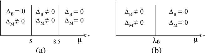
Figure 1: The phase diagram calculated in IT model in cold dense matter. Here energy dimension of chemical potential is arbitrary.

3 Field Theory Model For Competitions Between $\langle\bar{\psi}\psi\rangle$, $\langle\psi\psi\rangle$ And $\langle\psi^{\dagger}\psi\rangle$

In this section, we shall study a field-theory model by generalizing the model considered recently by Chodos et al [15] to one that contains a number density field corresponding to $\langle\psi^{\dagger}\psi\rangle$. The (1+1)-dimensional toy model we shall consider is defined by the Lagrangian

$$L = i\bar{\psi}^{(i)}\not\!\partial\psi^{(i)}-\mu\psi^{\dagger}\psi+\frac{1}{2}g^{2}[\bar{\psi}^{(i)}\psi^{(i)}][\bar{\psi}^{(j)}\psi^{(j)}]$$ (35)

$$+2G^{2}[\bar{\psi}^{(i)}\gamma_{5}\psi^{(j)}][\bar{\psi}^{(i)}\gamma_{5}\psi^{(j)}]-2F^{2}[\bar{\psi}^{(i)}\gamma^{\mu}\psi^{(i)}][\bar{\psi}^{(j)}\gamma_{\mu}\psi^{(j)}]$$

where $i$ runs from 1 to $N$. The last term is the term we have added to the model of Chodos et al. We shall do a large $N$ approximation. We do a Hubbard-Stratanovich transformation using the auxiliary fields, $\phi$, $B$ and $V_{\mu}$ by adding the term

$$\Delta L = -\frac{1}{2g^{2}}[\phi+g^{2}\bar{\psi}^{(i)}\psi^{(i)}]^{2}-\frac{1}{G^{2}}(B^{\dagger}-G^{2}\epsilon_{\alpha\beta}\psi_{\alpha}^{\dagger(i)}\psi_{\beta}^{\dagger(i)})(B+G^{2}\epsilon_{\gamma\delta}\psi_{\gamma}^{(i)}\psi_{\delta}^{(i)})$$ (36)

$$+\frac{2}{F^{2}}[V_{\mu}+F^{2}\bar{\psi}^{(i)}\gamma_{\mu}\psi^{(i)}]^{2}.$$

The resulting Lagrangian $L^{\prime}=L+\Delta L$ is

$$L^{\prime} = \bar{\psi}^{(i)}(i\not\!\partial-\phi-\mu\gamma_{0}+4\not\!V)\psi^{(i)}-\frac{\phi^{2}}{2g^{2}}-\frac{B^{\dagger}B}{G^{2}}+\frac{2}{F^{2}}V_{\mu}V^{\mu}$$ (37)

$$+B\epsilon_{\alpha\beta}\psi_{\alpha}^{\dagger(i)}\psi_{\beta}^{\dagger(i)}-B^{\dagger}\epsilon_{\alpha\beta}\psi_{\alpha}^{(i)}\psi_{\beta}^{(i)}.$$

We can now integrate out $\psi$ and $\psi^{\dagger}$ to obtain the effective action (modulo a constant)

$$\Gamma_{eff}(\phi,B,B^{\dagger},V_{0}) = \int d^{2}x(-\frac{\phi^{2}}{2g^{2}}-\frac{B^{\dagger}B}{G^{2}}+\frac{2}{F^{2}}V_{0}^{2})-\frac{i}{2}\rm Tr\ln(A^{T}A)$$ (38)

$$-\frac{i}{2}\rm Tr\ln[1+M^{2}(A^{T})^{-1}\sigma_{2}A^{-1}\sigma_{2}]$$

where we have assumed that $B$, $B^{\dagger}$, $\phi$ and $V_{0}$ are constant since we are interested in an effective potential with translation invariance and have defined

$$M^{2} = 4B^{\dagger}B$$

$$A = i\partial_{0}+i\sigma_{3}\partial_{3}-\tilde{\mu}-\phi\sigma_{1}$$

$$A^{T} = -i\partial_{0}-i\sigma_{3}\partial_{3}-\tilde{\mu}-\phi\sigma_{1}$$

with $\tilde{\mu}=\mu-4V_{0}$.

Factoring out $N$ coming from the flavor trace, we write $g^{2}N=\lambda$, $G^{2}N=\frac{\kappa}{4}$ and $F^{2}N=2\alpha$ and define $V_{eff}$ as $\Gamma_{eff}=-N(\int d^{2}x)V_{eff}$:

$$V_{eff}=\frac{\phi^{2}}{2\lambda}+\frac{M^{2}}{\kappa}-\frac{V_{0}^{2}}{\alpha}+V_{eff}^{(1)}$$ (39)

where $V_{eff}^{(1)}=\frac{i}{2}[\rm Tr\ln(A^{T}A)+\rm Tr\ln(1+M^{2}(A^{T})^{-1}\sigma_{2}A^{-1}\sigma_{2})]$. Then the gap equations are obtained by

$$\frac{\partial V_{eff}}{\partial\phi^{2}}=\frac{\partial V_{eff}}{\partial M^{2}}=\frac{\partial V_{eff}}{\partial V_{0}^{2}}=0$$ (40)

from which we get

$$\frac{1}{2\lambda} = -\frac{\partial V_{eff}^{(1)}}{\partial\phi^{2}}=i\int\frac{d^{2}k}{(2\pi)^{2}}\frac{[k_{0}^{2}-k_{1}^{2}+\tilde{\mu}^{2}+M^{2}-\phi^{2}]}{D}$$

$$\frac{1}{\kappa} = -\frac{\partial V_{eff}^{(1)}}{\partial M^{2}}=i\int\frac{d^{2}k}{(2\pi)^{2}}\frac{[k_{0}^{2}-k_{1}^{2}-\tilde{\mu}^{2}-M^{2}+\phi^{2}]}{D}$$

$$\frac{1}{\alpha} = \frac{\partial V_{eff}^{(1)}}{\partial V_{0}^{2}}=i\int\frac{d^{2}k}{(2\pi)^{2}}\frac{4\tilde{\mu}[k_{0}^{2}+k_{1}^{2}-\tilde{\mu}^{2}-M^{2}+\phi^{2}]}{V_{0}D}$$ (41)

where $D=[k_{0}^{2}-k_{1}^{2}-\tilde{\mu}^{2}-M^{2}+\phi^{2}]^{2}-4[\phi^{2}k_{0}^{2}+\mu^{2}k_{1}^{2}-\phi^{2}k_{1}^{2}]$ with $k_{0}=k_{0}+i\epsilon\ {\rm sgn}k_{0}$. After the $k_{0}$ integral, we have

$$\frac{1}{2\lambda} = \frac{1}{8\pi}\int_{-\Lambda}^{\Lambda}dk_{1}[\frac{1}{k_{+}}+\frac{1}{k_{-}}+\frac{M^{2}+\tilde{\mu}^{2}}{\sqrt{M^{2}\phi^{2}+\tilde{\mu}^{2}(k_{1}^{2}+\phi^{2})}}(\frac{1}{k_{+}}-\frac{1}{k_{-}})]$$

$$\frac{1}{\kappa} = \frac{1}{8\pi}\int_{-\Lambda}^{\Lambda}dk_{1}[\frac{1}{k_{+}}+\frac{1}{k_{-}}+\frac{\phi^{2}}{\sqrt{M^{2}\phi^{2}+\tilde{\mu}^{2}(k_{1}^{2}+\phi^{2})}}(\frac{1}{k_{+}}-\frac{1}{k_{-}})]$$

$$\frac{1}{\alpha} = \frac{\tilde{\mu}}{V_{0}}\frac{1}{2\pi}\int_{-\Lambda}^{\Lambda}dk_{1}[\frac{1}{k_{+}}+\frac{1}{k_{-}}+\frac{\phi^{2}+k_{1}^{2}}{\sqrt{M^{2}\phi^{2}+\tilde{\mu}^{2}(k_{1}^{2}+\phi^{2})}}(\frac{1}{k_{+}}-\frac{1}{k_{-}})]$$

where $\Lambda$ is a cutoff to regularize logarithmic divergences
and $k_{\pm}=\sqrt{M^{2}+\phi^{2}+\tilde{\mu}^{2}+k_{1}^{2}\pm 2\sqrt{M^{2}\phi^{2}+\tilde{\mu}^{2}(k_{1}^{2}+\phi^{2})}}$.

By integrating with respect to $\phi^{2}$, $M^{2}$ and $V_{0}^{2}$, we have the unrenormalized $V_{eff}^{(1)}$,

$$V_{eff}^{(1)}=-\frac{1}{2\pi}\int_{0}^{\Lambda}dk_{1}[k_{+}-k_{-}+c(k_{1})]+C(\mu)$$ (42)

where $c(k_{1})$ and $C(\mu)$, the value of which are determined later, are constants of integration. In the unrenormalized effective potential in free space, there can be quadratic and logarithmic divergences. Since free-space renormalization will eliminate all deivergences even in medium, we will cancel out the quadractic diverence by choosing a suitable value of $c(k_{1})$ and define renormalized coupling constants to eliminate logarithmic divergences. To be explicit, we take $\mu=0$. Then the $V_{eff}^{(1)}$ is given by

$$V_{eff}^{(1)} = -\frac{1}{2\pi}\int_{0}^{\Lambda}dk_{1}[\sqrt{M^{2}+\phi^{2}+16V_{0}^{2}+k_{1}^{2}+2\sqrt{M^{2}\phi^{2}+16V_{0}^{2}(k_{1}^{2}+\phi^{2})}}$$ (43)

$$+\sqrt{M^{2}+\phi^{2}+16V_{0}^{2}+k_{1}^{2}-2\sqrt{M^{2}\phi^{2}+16V_{0}^{2}(k_{1}^{2}+\phi^{2})}}-2k_{1}]$$

where we have chosen $c(k_{1})=-2k_{1}$ to cancel the quadratic divergence, see (44) and $C(\mu=0)=0$, see (51).

3.1 $\phi=0,~{}\mu=0$

Since it is not so easy to integrate (43) explicitly to separate the infinities from finite quantities, let us first confine ourselves to the case of $\phi=0$ . The $V_{eff}^{(1)}$ is given by

$$V_{eff}^{(1)}(V_{0},M) = -\frac{1}{2\pi}\int_{0}^{\Lambda}dk_{1}[\sqrt{M^{2}+(4V_{0}+k_{1})^{2}}+\sqrt{M^{2}+(4V_{0}-k_{1})^{2}}-2k_{1}]$$ (44)

$$= -\frac{1}{4\pi}[(\Lambda+4V_{0})\sqrt{(\Lambda+4V_{0})^{2}+M^{2}}+(\Lambda-4V_{0})\sqrt{(\Lambda-4V_{0})^{2}+M^{2}}$$

$$+M^{2}\ln\frac{\Lambda+4V_{0}+\sqrt{(\Lambda+4V_{0})^{2}+M^{2}}}{4V_{0}+\sqrt{16V_{0}^{2}+M^{2}}}$$

$$+M^{2}\ln\frac{\Lambda-4V_{0}+\sqrt{(\Lambda-4V_{0})^{2}+M^{2}}}{-4V_{0}+\sqrt{16V_{0}^{2}+M^{2}}}-2\Lambda^{2}].$$

The unrenormalized effective potential is given by

$$V_{eff}(V_{0},M) = M^{2}(\frac{1}{\kappa}-\frac{1}{4\pi})-V_{0}^{2}(\frac{1}{\alpha}+\frac{8}{\pi})$$ (45)

$$-\frac{1}{4\pi}[M^{2}\ln\frac{\Lambda+4V_{0}+\sqrt{(\Lambda+4V_{0})^{2}+M^{2}}}{4V_{0}+\sqrt{16V_{0}^{2}+M^{2}}}$$

$$+M^{2}\ln\frac{\Lambda-4V_{0}+\sqrt{(\Lambda-4V_{0})^{2}+M^{2}}}{-4V_{0}+\sqrt{16V_{0}^{2}+M^{2}}}].$$

We define the renormalized couplings $\kappa_{R}$ and $\alpha_{R}$ as

$$\frac{\partial^{2}V_{eff}}{\partial B\partial B^{\dagger}}|_{M=M_{0},V_{0}=v_{0}}=\frac{4}{\kappa_{R}},~{}~{}~{}\frac{\partial^{2}V_{eff}}{\partial V_{0}^{2}}|_{M=M_{0},V_{0}=v_{0}}=-\frac{2}{\alpha_{R}}$$ (46)

and get

$$\frac{1}{\alpha_{R}} = \frac{1}{\alpha}+\frac{8}{\pi}$$

$$\frac{1}{\kappa_{R}} = \frac{1}{\kappa}-\frac{1}{4\pi}[\ln\frac{\Lambda+4v_{0}+\sqrt{(\Lambda+4v_{0})^{2}+M_{0}^{2}}}{4v_{0}+\sqrt{16v_{0}^{2}+M_{0}^{2}}}$$ (47)

$$+\ln\frac{\Lambda-4v_{0}+\sqrt{(\Lambda-4v_{0})^{2}+M_{0}^{2}}}{-4v_{0}+\sqrt{16v_{0}^{2}+M_{0}^{2}}}-1].$$

The renormalized effective potential is now found to be

$$V_{eff}^{R}=M^{2}(\frac{1}{\kappa_{R}}-\frac{1}{2\pi})-V_{0}^{2}\frac{1}{\alpha_{R}}+\frac{M^{2}}{4\pi}\ln\frac{M^{2}}{M_{0}^{2}}.$$ (48)

Note that $V_{0}$ and $M$ are not coupled to each other. Solving the gap equations for $V_{0}$ and $M$, we obtain

$$V_{0} = 0$$

$$M^{2} = M_{0}^{2}e^{1-\frac{4\pi}{\kappa_{R}}}~{}~{}{\rm or}~{}~{}0.$$ (49)

At the solutions, the effective potential becomes

$$V_{eff}^{R} = 0~{}{\rm for}~{}V_{0}=0,~{}M^{2}=0$$

$$V_{eff}^{R} = -\frac{M_{0}^{2}}{4\pi}e^{1-\frac{4\pi}{\kappa_{R}}}~{}{\rm for}~{}V_{0}=0,~{}M^{2}\neq 0.$$ (50)

So the phase with $V_{0}=0,~{}M^{2}\neq 0$ is energetically favored and is a global minimum when $\alpha_{R}<0$.

3.2 $\phi=0$, $\mu\neq 0$

In this case, the renormalized effective potential is given (up to a constant) by

$$V_{eff}^{R}=M^{2}(\frac{1}{\kappa_{R}}-\frac{1}{2\pi})-V_{0}^{2}\frac{1}{\alpha_{R}}-\frac{1}{2\pi}\mu^{2}+\frac{4}{\pi}\mu V_{0}+\frac{M^{2}}{4\pi}\ln\frac{M^{2}}{M_{0}^{2}}+C(\mu)$$ (51)

where $C(\mu)$ will be fixed by the condition that $V_{eff}^{R}(M=0,V_{0}=0)=0$. We will make use of the condition $V_{eff}^{R}(M=0,V_{0}=0)=0$ throughout this paper. Then we have the renormalized effective potential,

$$V_{eff}^{R}=M^{2}(\frac{1}{\kappa_{R}}-\frac{1}{2\pi})-V_{0}^{2}\frac{1}{\alpha_{R}}+\frac{4}{\pi}\mu V_{0}+\frac{M^{2}}{4\pi}\ln\frac{M^{2}}{M_{0}^{2}}.$$ (52)

As far as $M^{2}$ is concerned, our effective potential is the same as that in Ref. [15]. Note that since $V_{0}$ and $M$ do not couple, it is easy to find solutions of the gap equations. We find

$$V_{0} = 2\frac{\alpha_{R}}{\pi}\mu,~{}~{}M^{2}=0~{}~{}{\rm or}$$ (53)

$$V_{0} = 2\frac{\alpha_{R}}{\pi}\mu,~{}~{}M^{2}=M_{0}^{2}e^{1-\frac{4\pi}{\kappa_{R}}}.$$ (54)

At the solutions, the effective potential becomes

$$V_{eff}^{R} = \frac{4}{\pi^{2}}\alpha_{R}\mu^{2}~{}{\rm for}~{}V_{0}=\alpha_{R}\frac{2}{\pi}\mu,~{}M^{2}=0$$

$$V_{eff}^{R} = \frac{4}{\pi^{2}}\alpha_{R}\mu^{2}-\frac{M_{0}^{2}}{4\pi}e^{1-\frac{4\pi}{\kappa_{R}}}~{}{\rm for}~{}V_{0}=\alpha_{R}\frac{2}{\pi}\mu,~{}M^{2}\neq 0.$$ (55)

From (55), we can see that the phase with $M\neq 0$ is energetically favored regardless of the behavior of $V_{0}$. Thus we expect there could exist a phase where superconductivity and mean fields coexist in the case of $M_{0}^{2}\neq 0$ at finite density. Since we are expecting superconductivity at high density, it is plausible that we have $M_{0}^{2}\neq 0$ with $M_{0}$ being small at some relevant density.

3.3 $M=0,\mu=0$

In this case, $V_{eff}^{(1)}$ takes the form

$$V_{eff}^{(1)}=-\frac{1}{2\pi}\int_{0}^{\Lambda}dk_{1}[\mid\sqrt{\phi^{2}+k_{1}^{2}}+4V_{0}\mid+\mid\sqrt{\phi^{2}+k_{1}^{2}}-4V_{0}\mid-2k_{1}].$$ (56)

We can consider two cases:

$\bullet$ $|\phi|>4|V_{0}|$:
In this case, the effective potential $V_{eff}^{(1)}$ is independent of $V_{0}$. Using the exactly same method adopted in the previous section, we have

$$\frac{1}{\lambda} = \frac{1}{\lambda_{R}}+\frac{1}{\pi}\ln\frac{\Lambda+\sqrt{\Lambda^{2}+\phi^{2}}}{\phi_{0}}-\frac{1}{\pi}$$ (57)

$$\frac{1}{\alpha} = \frac{1}{\alpha_{R}}$$ (58)

$$V_{eff}^{R} = \phi^{2}(\frac{1}{2\lambda_{R}}-\frac{3}{4\pi})-\frac{1}{\alpha_{R}}V_{0}^{2}+\frac{\phi^{2}}{4\pi}\ln\frac{\phi^{2}}{\phi_{0}^{2}}$$ (59)

where $\lambda_{R}$ is defined by $\frac{\partial^{2}V_{eff}}{\partial\phi^{2}}\mid_{M=M_{0},\phi=\phi_{0}}=\frac{1}{\lambda_{R}}$. Since $\alpha$ and $\alpha_{R}$ differ by a constant, we will use, hereafter, $\alpha$ instead of $\alpha_{R}$ just for simplicity. The solutions of the gap equations are given by

$$V_{0} = 0,~{}~{}\phi=0$$ (60)

$$~{}{\rm or}~{}V_{0} = 0,~{}~{}\phi=\phi_{0}e^{1-\frac{\pi}{\lambda_{R}}}.$$ (61)

It can be easily seen that the phase with $V_{0}=0$ and $\phi\neq 0$, at which $V_{eff}^{R}=-\frac{1}{4\pi}\phi_{0}^{2}e^{2-\frac{2\pi}{\lambda_{R}}}$, is favored. This comes as no surprise.

$\bullet$ $|\phi|<4|V_{0}|$:
We find

$$\frac{1}{\alpha} = \frac{1}{\alpha_{R}}-\frac{2}{\pi}\frac{16|v_{0}|}{\sqrt{16v_{0}^{2}-\phi_{0}^{2}}}$$

$$\frac{1}{\lambda} = \frac{1}{\lambda_{R}}+\frac{1}{\pi}\ln\frac{\Lambda+\sqrt{\Lambda^{2}+\phi_{0}^{2}}}{4|v_{0}|+\sqrt{16v_{0}^{2}-\phi_{0}^{2}}}+\frac{1}{\pi}\frac{\phi_{0}^{2}}{16v_{0}^{2}-\phi_{0}^{2}+4|v_{0}|\sqrt{16v_{0}^{2}-\phi_{0}^{2}}}$$

$$V_{eff}^{R} = \phi^{2}(\frac{1}{2\lambda_{R}}-\frac{1}{4\pi})-\frac{1}{\alpha}V_{0}^{2}$$ (62)

$$+\frac{1}{2\pi}\phi^{2}\ln\frac{4|V_{0}|+\sqrt{16V_{0}^{2}-\phi^{2}}}{4|v_{0}|+\sqrt{16v_{0}^{2}-\phi_{0}^{2}}}$$

$$+\frac{1}{2\pi}\phi^{2}\frac{\phi_{0}^{2}}{16v_{0}^{2}-\phi_{0}^{2}+4|v_{0}|\sqrt{16v_{0}^{2}-\phi_{0}^{2}}}-\frac{2}{\pi}|V_{0}|\sqrt{16V_{0}^{2}-\phi^{2}}.$$

Solving the gap equations, we find that the only possible solutions are $V_{0}=0$ and $\phi=0$ where $V_{eff}^{R}=0$. So at zero chemical potential, the system is again characterized by $V_{0}=0$ and $\phi\neq 0$.

3.4 $M=0,\mu\neq 0$

$\bullet$ $|\phi|>4|V_{0}|$:
For $\mu<\mid\phi\mid$, the effective potential is equal to (59). In this case, our system is characterized by

$$V_{0}=0,~{}~{}\phi=\phi_{0}e^{1-\frac{\pi}{\lambda_{R}}}.$$ (63)

For $\mu>\mid\phi\mid$, we have

$$V_{eff}^{R} = \phi^{2}(\frac{1}{2\lambda_{R}}-\frac{3}{4\pi})-\frac{1}{\alpha}V_{0}^{2}-\frac{1}{2\pi}\tilde{\mu}\sqrt{\tilde{\mu}^{2}-\phi^{2}}$$ (64)

$$-\frac{1}{2\pi}\phi^{2}\ln\frac{\phi_{0}}{\tilde{\mu}+\sqrt{\tilde{\mu}^{2}-\phi^{2}}}+\frac{1}{2\pi}\mu^{2}.$$

(Recall that $\tilde{\mu}=\mu-4V_{0}$.) The possible solutions of the gap equations are calculated to be

$$V_{0} = -\frac{1}{\frac{\pi}{2\alpha}-4}(\mu-\phi_{0}e^{1-\frac{\pi}{\lambda_{R}}})$$

$$\phi^{2} = \tilde{\mu}^{2}-\frac{\pi^{2}}{4\alpha^{2}}V_{0}^{2}.$$ (65)

At the solutions of the gap equations, we have

$$V_{eff}^{R}=\frac{1}{4\pi}\mu^{2}+(\frac{2}{\pi}-\frac{1}{4\alpha_{R}})\mu V_{0}-\frac{1}{4\pi}(16-\frac{\pi^{2}}{4\alpha_{R}^{2}})V_{0}^{2}.$$ (66)

$\bullet$ $|\phi|<4|V_{0}|$:

$$V_{eff}^{R} = \phi^{2}(\frac{1}{2\lambda_{R}}-\frac{1}{4\pi})-\frac{1}{\alpha}V_{0}^{2}$$ (67)

$$+\frac{1}{2\pi}\phi^{2}\ln\frac{\mid\tilde{\mu}\mid+\sqrt{\tilde{\mu}^{2}-\phi^{2}}}{4v_{0}+\sqrt{16v_{0}^{2}-\phi_{0}^{2}}}+\frac{1}{2\pi}\mu^{2}$$

$$+\frac{1}{2\pi}\phi^{2}\frac{\phi_{0}^{2}}{16v_{0}^{2}-\phi_{0}^{2}+4|v_{0}|\sqrt{16v_{0}^{2}-\phi_{0}^{2}}}-\frac{1}{2\pi}\mid\tilde{\mu}\mid\sqrt{\tilde{\mu}^{2}-\phi^{2}}.$$

First, we consider the case of

$$\phi=0~{}{\rm and}~{}V_{0}=\frac{1}{\frac{\pi}{2\alpha}+4}\mu$$ (68)

which is one of the solutions of the gap equations. In this case, the effective potential becomes

$$V_{eff}^{R}=-\frac{1}{2\pi}(16+\frac{2\pi}{\alpha})V_{0}^{2}+\frac{4}{\pi}V_{0}\mu.$$ (69)

For $\tilde{\mu}>0$, we have the following solution for the gap equation

$$V_{0} = -\frac{1}{\frac{\pi}{2\alpha}-4}[\mu-C_{1}e^{-(\frac{\pi}{\lambda_{R}}+C_{2})}]$$

$$\phi^{2} = \tilde{\mu}^{2}-\frac{\pi^{2}}{4\alpha^{2}}V_{0}^{2}.$$ (70)

In the case of $\tilde{\mu}<0$, we have

$$V_{0} = -\frac{1}{\frac{\pi}{2\alpha}-4}[\mu+C_{1}e^{-(\frac{\pi}{\lambda_{R}}+C_{2})}]$$

$$\phi^{2} = \tilde{\mu}^{2}-\frac{\pi^{2}}{4\alpha^{2}}V_{0}^{2}.$$ (71)

To see which phase is energetically favorable, we take $\phi_{0}=m_{F}$ and $M_{0}\approx 0$ .

In free space ($\mu=0$), we have two phases:

$$V_{eff}^{R} = -\frac{1}{4\pi}m_{F}^{2}e^{2-\frac{2\pi}{\lambda_{R}}}~{}{\rm for}~{}V_{0}=0~{}{\rm and}~{}\phi\neq 0$$

$$V_{eff}^{R} = -\frac{M_{0}^{2}}{4\pi}e^{1-\frac{4\pi}{\kappa_{R}}}~{}{\rm for}~{}V_{0}=0~{}{\rm and}~{}M\neq 0.$$ (72)

Since $M_{0}$ will be zero or small, our system sits in the phase with $V_{0}=0$ and $\phi\neq 0$. In free space, therefore, we have chiral symmetry breaking but no superconductivity.

At finite density, the situation becomes more complicated. We have six sets of solutions of the gap equation: (54), (63), (65), (68), (70) and (71). Now let us investigate the competition between the phases characterized by (54), (63) and (68). The effective potentials given at their ground-state positions are

$$I~{}:~{}V_{eff}^{R} = \frac{4}{\pi^{2}}\frac{1}{\frac{1}{\alpha}+\frac{8}{\pi}}\mu^{2}-\frac{M_{0}^{2}}{4\pi^{2}}e^{1-\frac{4\pi}{\kappa_{R}}}~{}\leftrightarrow~{}(\ref{v35})$$

$$II~{}:~{}V_{eff}^{R} = -\frac{1}{4\pi}m_{F}^{2}e^{2-\frac{2\pi}{\lambda_{R}}}~{}\leftrightarrow~{}(\ref{v42})$$

$$III~{}:~{}V_{eff}^{R} = \frac{4}{\pi^{2}}\frac{1}{\frac{1}{\alpha}+\frac{8}{\pi}}\mu^{2}~{}\leftrightarrow~{}(\ref{gs2}).$$ (73)

Comparing $I$ and $III$, we find that our system will be in the mixed phase ($I$) characterized by $\langle\psi^{\dagger}\psi\rangle\neq 0$ and $\langle\psi\psi\rangle\neq 0$ as long as $M_{0}^{2}\neq 0$. From the condition that the phase $I$ is the global minimum of the potential (52), $\frac{1}{\alpha}+\frac{8}{\pi}<0$, we find $-0.125\pi<\alpha<0$. It is expected that the phase $II$, which is valid when $\mu<|\phi|$, becomes the absolute minimum of the potential at low density. To see the competition between $I$ and $II$ explicitly, we neglect a term with $M_{0}^{2}$ in the phase I and take $\lambda_{R}=\pi$ and $\alpha=-0.1\pi$. Then we find $\frac{\mu_{c}}{m_{F}}\approx 0.4$. In the regime $\mu<\mu_{c}$, we have the chiral symmetry breaking phase ($II$) with almost zero fermion number density defined by $\rho_{F}=-\frac{\partial V_{R}^{eff}}{\partial\tilde{\mu}}$. In the case of $\mu>\mu_{c}$ the system sits in the mixed phase ($I$) with fermion number density

$$\rho_{F} = -\frac{8\alpha_{R}}{\pi^{2}-8\pi\alpha_{R}}\mu~{}~{}{\rm with}~{}\frac{1}{\alpha_{R}}=\frac{1}{\alpha}+\frac{8}{\pi}$$ (74)

$$\approx 0.25\mu~{}{\rm for}~{}\alpha=-0.1\pi.$$

The fermion number density is depicted in Fig. 2. We should, however, consider competitions with other possible phases. To investigate numerically the phases characterized by (65), (70) and (71), we take the following parameters

$$\lambda_{R} = \pi$$

$$\alpha = -\pi,~{}-0.1\pi$$

$$\frac{v_{0}}{\phi_{0}} = 10,~{}1.0,~{}0.3~{}.$$ (75)

With this parameter choice, we plot the renormalized effective potentials near the minimum-energy positions (i.e., solutions of the gap equations), (65), (70) and (71). We find that the phases characterized by (65), (70) and (71) correspond to the maximum or saddle point of the renormalized effective potential or does not satisfy some constraints, for example $4|V_{0}|>|\phi|$, near the minimum-energy positions and therefore those phases are unstable or an unphysical “vacuum.”

Figure 2: Fermion number density as a function of chemical potential. Here $\bar{\rho}\equiv\frac{\rho_{F}}{m_{F}}$ and $\bar{\mu}\equiv\frac{\mu}{m_{F}}$. In the regime $\mu<\mu_{c}$ the system sits in the chiral symmetry breaking phase($II$) and in the mixed phase phase($I$) in the case of $\mu>\mu_{c}$.

4 Conclusion

We studied the competitions between induced symmetry breaking (ISB), Cooper pairing condensate and chiral condensate at finite baryon density.

By reformulating the IT model [10] using the Bogoliubov-Valatin transformation, we show that the mixed phase, in which both $\Delta_{M}$ and $\Delta_{B}$ are non-zero, is energetically favored. By symmetry we argue that the ISB phenomena may not be a relevant notion in the IT model.

We calculated the effective potentials $V(\phi=0,V_{0},M)$ and $V(M=0,V_{0},\phi)$ which are functions of the fermion-antifermion (or chiral), ISB (or mean-field) and Cooper-pairing order parameters $\phi$, $V_{0}$ and $M$, respectively. At zero chemical potential, we find that the global minimum of the effective potential is given by $V_{0}=0$ and $M\neq 0$ or $V_{0}=0$ and $\phi\neq 0$. Since $M_{0}$ should be zero [15] or very small, it is reasonable to conclude that the system sits in the chiral symmetry breaking phase.

At finite density, taking $\lambda_{R}=\pi$ and $\alpha=-0.1\pi$, we find that in the regime $\mu<\mu_{c}$, we have the chiral symmetry breaking phase(II) with almost zero fermion number density and in the case of $\mu>\mu_{c}$ the system sits in the mixed phase with nonzero “vacuum” (or rather ground-state) expectation values of $\langle\psi^{\dagger}\psi\rangle$ and $\langle\psi\psi\rangle$, i.e, $V_{0}\neq 0$ and $M\neq 0$. We observe an ISB-like behavior in the fermion number density as in fig. 2 but we fail to observe the exclusive competition obtained in [4]. As we can see in (54) and also in ref.[15], $M$ ($\sim\langle\psi\psi\rangle$) is independent of the chemical potential. We are unable to say whether or not these are an artifact of the simplified models not present in effective theories of QCD. A similar (uncertain) situation applies also to analysis made in QCD at weak coupling[17].

Our analysis depends on the value of the renomalization point which is arbitrary in general. The possible resolution to this arbitrariness is to do a renormalization group analysis at finite density discussed in [16]. Such a procedure will replace the renormalization scale (up to a constant) by the chemical potential[16]. We leave this exercise to a future publication.

Appendix

In this appendix, we compare the grand canonical ensemble used in this work and in ref.[10, 11] (case B) with that widely used in BCS theory, for example see [18] (case A). Here ($a,a^{*}$) stand for the annihilation and creation operators for the “bare” fermions and ($b,b^{*}$) for the quasiparticles as in section 2.

$\Delta_{B}\neq 0,~{}\Delta_{M}=0$

Here we shall take the mean-field gap to be zero, i.e., $\Delta_{M}=0$ for simplicity. Since the BCS ground state does not preserve the particle number of the ground state, a condition is imposed on the average;

$$\langle\Psi_{BCS}|N_{op}|\Psi_{BCS}\rangle=\bar{N}$$ (76)

where $N_{op}=\sum_{k}a^{*}_{k}a_{k}$, the number operator. As described in ref.[18] in detail, this relaxation of the condition of $N$ in the BCS and Bogoliubov theory must be distinguished from the use of grand canonical ensemble in statistical mechanics. In grand canonical ensemble of statistical mechanics, we deal with an ensemble of systems, with a distribution of particle numbers $N$ with the systems with N particles being weighted by a factor $z^{N}$ where $z$ called fugacity is defined by $z=e^{\beta\mu}$. However, each separate system within an assembly has its own definite number of particles $N$.

In the case of A, we add a term $-\mu_{a}a^{*}a$ to the Hamiltonian to specify the mean value of particle number. Normally in this case, we adjust the chemical potential $\mu$ to satisfy $\langle N_{a}\rangle={\bar{N}}_{a}$. Here the chemical potential $\mu_{a}$ is a variable conjugate to $N_{a}=\sum_{k}a^{*}_{k}a_{k}$. After specifying the mean number of $N_{a}$, we diagonalize the Hamiltonian to get $H(b^{*}b)$ describing quasi-particles. We can specify a constant number (in the sense of the average given above) to a system characterized by this diagonalized Hamiltonian $H(b^{*}b)$. Therefore this system becomes effectively canonical ensemble of the statistical system with definite number but we are essentially using the grand canonical ensemble. Then the probability of quasi-particle thermal excitation is given at a given energy $\epsilon$ by $\langle b^{*}b\rangle=(1+e^{\beta\sqrt{(\epsilon-\mu_{a})^{2}+\Delta_{B}^{2}}})^{-1}$.

In the case of B, we do not constrain the mean number in terms of $N_{a}=\sum_{k}a^{*}_{k}a_{k}$. Since our diagonalized Hamiltonian $H(b^{*}b)$ has the same structure with that of non-interacting harmonic oscillator and preserves the particle number, we can define a simultaneous eigenstate of quasi-particle number and energy operators . Note that the quasiparticle operator $b$ kills, by definition, the BCS ground state $b|\Psi_{BCS}\rangle=0$ and the lowest quasiparticle excitation state is given by $b^{*}|\Psi_{BCS}\rangle$. Following an elementary procedure in statistical mechanics, we have $\langle b^{*}b\rangle=(e^{\beta(\sqrt{\epsilon^{2}+\Delta_{B}^{2}}-\mu_{b})}+1)^{-1}$ with $\mu_{b}$ being the “chemical potential” for quasiparticles. This formalism B is essential if we want to consider both $\lambda_{B}>0$ and $\lambda_{B}<0$ on the same footing. If we use the formalism A, the gap equation becomes

$$\sqrt{(\epsilon-\mu_{a})^{2}+\Delta_{B}^{2}}=\lambda_{B}\tanh\frac{\beta\sqrt{(\epsilon-\mu_{a})^{2}+\Delta_{B}^{2}}}{2}.$$ (77)

Taking $\beta\rightarrow\infty$, we have

$$\sqrt{(\epsilon-\mu_{a})^{2}+\Delta_{B}^{2}}=\lambda_{B}$$ (78)

showing that $\lambda_{B}<0$ does not enter into the consideration. Note that $\lambda_{B}>0$ corresponds to the usual BCS attraction.

Since the chemical potential $\mu_{b}$ essentially controls the number of quasiparticle excitations while the chemical potential $\mu_{a}$ fixes the mean number of the ground state, one might say that $\mu_{b}$ has nothing to do with $\mu_{a}$. But one should keep it in mind that $b^{*}$ is a linear combination of the $a$ and $a^{*}$ original fermion operators. Thus $b^{*}$ can create and annihilate fermions ($a,a^{*}$) from the ground state. This implies that controlling the number of quasi-particles must have something to do with that of the “bare” fermion $(a^{*},a)$. Whether we fix the number of ground state($A$) or quasi-particle excitation($B$), they should give the same answer for $\langle a^{*}a\rangle$. Note that $(a^{*},a)$ and $(b^{*},b)$ are connected by the canonical transformation:

$$\langle a^{*}(p)a(p)\rangle = \{\frac{c^{2}(p)}{1+e^{\beta(E-\mu_{b})}}+\frac{s^{2}(p)}{1+e^{-\beta(E-\mu_{b})}}\}~{}{\rm with}~{}E=\sqrt{\epsilon^{2}+\Delta_{B}^{2}}$$ (79)

$$= \{\frac{c^{2}(p)}{1+e^{\beta E}}+\frac{s^{2}(p)}{1+e^{-\beta E}}\}~{}{\rm with}~{}E=\sqrt{(\epsilon-\mu_{a})^{2}+\Delta_{B}^{2}}$$

where $\epsilon=p^{2}$.

$\Delta_{B}=0,~{}\Delta_{M}\neq 0$

In this case the probability of thermal excitation of “bare” fermion is given by (for $\epsilon+\Delta_{M}>\mu_{a}$)

$$\langle a^{*}(p)a(p)\rangle = \frac{1}{1+e^{\beta(\epsilon+\Delta_{M}-\mu_{b})}}~{}{\rm with}~{}B$$ (80)

$$= \frac{1}{1+e^{\beta(\epsilon+\Delta_{M}-\mu_{a})}}~{}{\rm with}~{}A$$

$$= \langle b^{*}(p)b(p)\rangle$$

showing $\mu_{a}=\mu_{b}$. Note that in the case $\Delta_{B}=0,~{}\Delta_{M}\neq 0$, the KMS-state is defined for the operator $(a,a^{*})$[10].

References

- [1] F. Wilczek, “ QCD in Extreme Conditions,” hep-ph/0003183; T. Schaefer, “Color Superconductivity,” nucl-th/9911017; K. Rajagopal, “ Mapping the QCD Phase Diagram,” hep-ph/9908360
- [2] K. Rajagopal and E. Shuster, “On the Applicability of Weak-Coupling Results in High Density QCD,” hep-ph/0004074
- [3] B.-Y. Park, M. Rho, A. Wirzba and I. Zahed, “Dense QCD: Overhauser or BCS pairing?”, hep-ph/9910347
- [4] K. Langfeld and M. Rho,”Quark Condensation, Induced Symmetry Breaking and Color Superconductivity at High Density ,” hep-ph/9811227, Nucl. Phys. A 660, 475 (1999) ; K. Langfeld, H. Reinhardt and M. Rho, Nucl. Phys. A622, 620 (1997)
- [5] S. Pepin, M. Birse, J.A. McGovern and N.R. Walet, “Nucleons or diquarks? Competition between clustering and color superconductivity in quark matter,” hep-ph/9912475
- [6] Y. Kim, R. Rapp, G.E. Brown and M. Rho, “A schematic model for - mixing at finite density and in-medium effective Lagrangian,’ nucl-th/9912061, Phys. Rev. C, in press
- [7] K. Langfeld, Nucl. Phys. A642, 96 (1998)
- [8] M. Alford, K. Rajagopal and F. Wilczek, Phys. Lett. B422, 247 (1998)
- [9] J. Berges, D.-U. Jungckel and C. Wetterich, ” The chiral phase transition at high baryon density from nonperturbative flow equations,” hep-ph/9811347, Eur. Phys. J. C13, 323 (2000)
- [10] N. Ilieva and W. Thirring, ”A pair potential supporting a mixed mean-filed/BCS-phase,” math-ph/9904027, Nucl. Phys. B565[FS], 629 (2000)
- [11] N. Ilieva and W. Thirring, “A mixed meanf-field/BCS phase with an energy gap at high ,” math-ph/0001023
- [12] N.D. Mermin and H. Wagner, Phys. Rev. Lett. 17, 1133 (1966); S. Coleman, Comm. Math. Phys. 31, 259 (1973)
- [13] E. Witten, Nucl. Phys. B145, 110 (1978)
- [14] N. N. Bogoliubov, Soviet Phys. JETP 7, 794 (1958) ; J. G. Valatin, Nuovo Cimento 7, 843 (1958)
- [15] A. Chodos, F. Cooper, W. Mao, H. Minakata and A. Singh, “A Two-dimensional Model with Chiral Condensates and Cooper Pairs having QCD-like Phase Structure,” hep-ph/9909296 ; A. Chodos, F. Cooper and H. Minakata, Phys. Lett. B449, 260 (1999)
- [16] J.C. Collins and M.J. Perry, Phys. Rev. Lett. 34, 1353 (1975); P.D. Morley and M.B. Kislinger, Phys. Rept. 51, 63 (1979); Y. Kim and H. K. Lee, “ Renormalization Group Analysis of -Meson Properties at Finite Density,” hep-ph/9905268, To be published in Phys. Rev. C
- [17] R. D. Pisarski, “Critical Line for H-Superfluidity in Strange Quark Matter?”, nucl-th/9912070
- [18] J. M. Blatt, Theory of Superconductivity (Academic Press, 1964)