NEUTRINO OSCILLATIONS AND THE SOLAR NEUTRINO PROBLEM

Abstract

I describe the current status of the solar neutrino problem, summarizing the arguments that its resolution will require new particle physics. The phenomenon of matter-enhanced neutrino oscillations is reviewed. I consider the implications of current experiments – including the SuperKamiokande atmospheric neutrino and LSND measurements – and the need for additional constraints from SNO and other new detectors.

1 Introduction

Part of the interest in neutrino astrophysics has to do with the fascinating interplay between nuclear and particle physics issues — e.g., whether neutrinos are massive and undergo flavor oscillations, whether they have detectable electromagnetic moments, etc. — and astrophysical phenomena, such as the clustering of matter on large scales, the processes responsible for the synthesis of nuclei, the mechanism for core-collapse supernovae, and the evolution of our sun. This summary addresses one of the oldest problems in neutrino astrophysics, the 30-year puzzle of the missing solar neutrinos. This puzzle grew out of attempts to test the standard theory of main sequence stellar evolution, but has now led to speculations about physics beyond the standard model of electroweak interactions. I will describe the work that defined the solar neutrino problem, the likelihood that its resolution is connected with massive neutrinos, and the hopes we have for future experiments.

2 Open Questions in Neutrino Physics [1]

The existence of the neutrino was first suggested by Wolfgang Pauli in a private letter dated December, 1930. The motivation was to solve an apparent problem with energy conservation in nuclear $\beta$ decay: the observable particles in the final state (the daughter nucleus and emitted electron) carried less energy than that released in the nuclear decay. Pauli suggested that an unobserved particle, the neutrino, accompanied the decay and accounted for the missing energy.

A number of important developments followed Pauli’s suggestion. In 1934 Fermi [2] suggested a theory of $\beta$ decay that was modeled after electromagnetism, except that there was no analog of the electromagnetic field: the interaction occurred at a point. (Apart from the missing aspect of parity violation, this was the correct reduction of today’s standard model to an effective theory.) In 1934 Bethe and Critchfield described the role of $\beta$ decay in thermonuclear reaction chains powering the stars

$$(A,Z)\rightarrow(A,Z-1)+e^{+}+\nu_{e}$$

thus predicting that our sun produces an enormous neutrino flux. In 1956 Cowan and Reines [3] succeeded in measuring neutrinos emitted by a reactor through the reaction

$$\bar{\nu}_{e}+p\rightarrow n+e^{+},$$

exploiting the positron and neutron coincidence. (The neutron was detected by $(n,\gamma)$ on a Cd neutron poison.) In 1957 the weak force mediating neutrino interactions was found to violate parity maximally. Later experiments found that the $\nu_{e}$ was replicated twice more in nature – the $\nu_{\mu}$ and $\nu_{\tau}$ – each accompanying a distinct charged lepton,

$$\nu_{e}\leftrightarrow e^{-}~{}~{}~{}\nu_{\mu}\leftrightarrow\mu^{-}~{}~{}~{}\nu_{\tau}\leftrightarrow\tau^{-}.$$

Finally all of this physics was embodied in the standard electroweak model, out of which came the prediction of a new neutral interaction mediating neutrino scattering.

Despite all of this progress, a remarkable number of questions remain. We now believe neutrinos are massive, but still have no measurement of an absolute neutrino mass (only mass differences). Many models attribute the puzzle of neutrino mass — why these neutrinos are so much lighter than other standard model particles — to scales well beyond the standard model, but we lack independent experimental tools for probing these scales. We do not now the particle-antiparticle conjugation properties of neutrinos: because they carry no standard model charges, both the Dirac (distinct antiparticle) and Majorana (no distinction between particle and antiparticle) possibilities are open. An associated question is the existence of nonzero electromagnetic moments: magnetic, charge radius, anapole, and electric dipole. No nonzero moment has been measured.

Finally, there are many questions about the role of neutrinos in astrophysics and cosmology. We suspect cosmic background neutrinos contribute to dark matter and may influence large-scale structure formation. However direct experimental attempts to measure background neutrinos have failed by many orders of magnitude to reach the expected density. Type II supernovae convert approximately 99% of the energy released in the infall into neutrinos of all flavors. Yet only $\bar{\nu}_{e}$s were detected from SN1987A. Supernova modelers predict that neutrinos play an essential role in the explosion mechanism and in the associated nucleosynthesis, yet there is disagreement about the success of neutrino-driven explosions. Finally, there is great interest in mounting searches for very high energy astrophysical neutrinos that might be associated with active galactic nuclei, gamma ray bursts, etc.

Given all of these open questions, 70 years after Pauli’s original suggestion, it would be nice to have a few more answers. There is every indication that some answers will come with the resolution of the solar neutrino puzzle.

3 The Standard Solar Model [4, 5]

Solar models trace the evolution of the sun over the past 4.7 billion years of main sequence burning, thereby predicting the present-day temperature and composition profiles of the solar core that govern neutrino production. Standard solar models (SSMs) share four basic assumptions:

* The sun evolves in hydrostatic equilibrium, maintaining a local balance between the gravitational force and the pressure gradient. To describe this condition in detail, one must specify the equation of state as a function of temperature, density, and composition.

* Energy is transported by radiation and convection. While the solar envelope is convective, radiative transport dominates in the core region where thermonuclear reactions take place. The opacity depends sensitively on the solar composition, particularly the abundances of heavier elements.

* Thermonuclear reaction chains generate solar energy. The standard model predicts that over 98% of this energy is produced from the pp chain conversion of four protons into ⁴He (see Fig. 1)

$$4p\rightarrow^{4}\mathrm{He}+2e^{+}+2\nu_{e}$$ (1)

with proton burning through the CNO cycle contributing the remaining 2%. The sun is a large but slow reactor: the core temperature, $T_{c}\sim 1.5\cdot 10^{7}$ K, results in typical center-of-mass energies for reacting particles of $\sim$ 10 keV, much less than the Coulomb barriers inhibiting charged particle nuclear reactions. Thus reaction cross sections are small: in most cases laboratory measurements are only possible at higher energies, so that cross section data must be extrapolated to the solar energies of interest.

* The model is constrained to produce today’s solar radius, mass, and luminosity. An important assumption of the standard model is that the sun was highly convective, and therefore uniform in composition, when it first entered the main sequence. It is furthermore assumed that the surface abundances of metals (nuclei with A $>$ 5) were undisturbed by the subsequent evolution, and thus provide a record of the initial solar metallicity. The remaining parameter is the initial ⁴He/H ratio, which is adjusted until the model reproduces the present solar luminosity in today’s sun. The resulting ⁴He/H mass fraction ratio is typically 0.27 $\pm$ 0.01, which can be compared to the big-bang value of 0.23 $\pm$ 0.01. Note that the sun was formed from previously processed material.

Figure 1: The solar pp chain.

The model that emerges is an evolving sun. As the core’s chemical composition changes, the opacity and core temperature rise, producing a 44% luminosity increase since the onset of the main sequence. The temperature rise governs the competition between the three cycles of the pp chain: the ppI cycle dominates below about 1.6 $\cdot 10^{7}$ K; the ppII cycle between (1.7-2.3) $\cdot 10^{7}$K; and the ppIII above 2.4 $\cdot 10^{7}$K. The central core temperature of today’s SSM is about 1.55 $\cdot 10^{7}$K.

The competition between the cycles determines the pattern of neutrino fluxes. Thus one consequence of the thermal evolution of our sun is that the ⁸B neutrino flux, the most temperature-dependent component, proves to be of relatively recent origin: the predicted flux increases exponentially with a doubling period of about 0.9 billion years.

A final aspect of SSM evolution is the formation of composition gradients on nuclear burning timescales. Clearly there is a gradual enrichment of the solar core in ⁴He, the ashes of the pp chain. Another element, ³He, can be considered a catalyst for the pp chain, being produced and then consumed, and thus eventually reaching some equilibrium abundance. The timescale for equilibrium to be established as well as the final equilibrium abundance are both sharply decreasing functions of temperature, and therefore increasing functions of the distance from the center of the core. Thus a steep ³He density gradient is established over time.

The SSM has had some notable successes. From helioseismology [6] the sound speed profile $c(r)$ has been very accurately determined for the outer 90% of the sun, and is in excellent agreement with the SSM. Such studies verify important predictions of the SSM, such as the depth of the convective zone. However the SSM is not a complete model in that it does not explain all features of solar structure, such as the depletion of surface Li by two orders of magnitude. This is usually attributed to convective processes that operated at some epoch in our sun’s history, dredging Li to a depth where burning takes place.

The principal neutrino-producing reactions of the pp chain and CNO cycle are summarized in Table 1. The first six reactions produce $\beta$ decay neutrino spectra having allowed shapes with endpoints given by E${}_{\nu}^{\rm max}$. Deviations from an allowed spectrum occur for ⁸B neutrinos because the ⁸Be final state is a broad resonance. The last two reactions produce line sources of electron capture neutrinos, with widths $\sim$ 2 keV characteristic of the temperature of the solar core. Measurements of the pp, ⁷Be, and ⁸B neutrino fluxes will determine the relative contributions of the ppI, ppII, and ppIII cycles to solar energy generation. As discussed above, and as later illustrations will show more clearly, this competition is governed in large classes of solar models by a single parameter, the central temperature $T_{c}$. The flux predictions of the 1998 calculations of Bahcall, Basu, and Pinsonneault [4] (BP98) and of Brun, Turck-Chieze and Morel [5] are included in Table 1.

Table 1: Solar neutrino sources and the flux predictions of the BP98 and Brun/Turck-Chieze/Morel SSMs in cm^-2s^-1.

Source	E${}_{\nu}^{max}$ (MeV)	BP98	BTCM98
p + p $\rightarrow^{2}$H + e${}^{+}+\nu$	0.42	5.94E10	5.98E10
13N $\rightarrow^{13}$C + e${}^{+}+\nu$	1.20	6.05E8	4.66E8
15O $\rightarrow^{15}$N + e${}^{+}+\nu$	1.73	5.32E8	3.97E8
17F $\rightarrow^{17}$O + e${}^{+}+\nu$	1.74	6.33E6
8B $\rightarrow^{8}$Be + e${}^{+}+\nu$	$\sim$ 15	5.15E6	4.82E6
3He + p $\rightarrow^{4}$He + e${}^{+}+\nu$	18.77	2.10E3
7Be + e${}^{-}\rightarrow^{7}$Li + $\nu$	0.86 (90%)	4.80E9	4.70E9
	0.38 (10%)
p + e- + p $\rightarrow^{2}$H + $\nu$	1.44	1.39E8	1.41E8

4 Solar Neutrino Experiments and their Implications

The first solar neutrino results were announced by Ray Davis Jr. and his Brookhaven collaborators in 1968, more than 30 years ago [7]. Located deep within the Homestake Gold Mine in Lead, South Dakota, the detector consists of a 100,000 gallon tank of C₂Cl₄. Solar neutrinos are captured by

$${}^{37}\mathrm{Cl}(\nu,e^{-})^{37}\mathrm{Ar}.$$

As the threshold for this reaction is 0.814 MeV, the important neutrino sources are the ⁷Be and ⁸B reactions. The ⁷Be neutrinos excite just the Gamow-Teller (GT) transition to the ground state, the strength of which is known from the electron capture lifetime of ³⁷Ar. The ⁸B neutrinos can excite all bound states in ³⁷Ar, including the dominant transition to the isobaric analog state residing at an excitation energy of 4.99 MeV. The strength of excite-state GT transitions can be determined from the $\beta$ decay ³⁷Ca$(\beta^{+})^{37}$K, which is the isospin mirror reaction to ³⁷Cl$(\nu,e^{-})^{37}$Ar. The net result is that, for SSM fluxes, 78% of the capture rate should be due to ⁸B neutrinos, and 15% to ⁷Be neutrinos. The measured capture rate [8] 2.56 $\pm 0.16\pm 0.16$ SNU (1 SNU = 10^-36 capture/atom/sec) is about one-third the SSM value.

Similar radiochemical experiments were begun in January, 1990, and May, 1991, respectively, by the SAGE and GALLEX collaborations using a different target, ⁷¹Ga. The special properties of this target include its low threshold and an unusually strong transition to the ground state of ⁷¹Ge, leading to a large pp neutrino cross section (see Fig. 2). The experimental capture rates are $66.6{}^{+6.8}_{-7.1}{}^{+3.8}_{-4.0}$ (SAGE) [9] and $77.5\pm 6.2{}^{+4.3}_{-4.7}$ SNU (GALLEX) [10]. The SSM prediction is about 130 SNU [11]. Most important, since the pp flux is directly constrained by the solar luminosity in all steady-state models, there is a minimum theoretical value for the capture rate of 79 SNU, given standard model weak interaction physics. Note there are substantial uncertainties in the ⁷¹Ga cross section due to ⁷Be neutrino capture to two excited states of unknown strength. These uncertainties were greatly reduced by direct calibrations of both detectors using ⁵¹Cr neutrino sources.

Figure 2: Level scheme for ⁷¹Ge showing the excited states that contribute to absorption of pp, ⁷Be, ⁵¹Cr and ⁸B neutrinos.

Experiments of a different kind, Kamiokande II/III and SuperKamiokande, exploit water Cerenkov detectors to view solar neutrinos event-by-event. Solar neutrinos scatter off electrons, with the recoiling electrons producing the Cerenkov radiation that is then recorded in surrounding phototubes. Thresholds are determined by background rates; SuperKamiokande is currently operating with a trigger at approximately six MeV. The initial experiment, Kamiokande II/III, found a flux of ⁸B neutrinos of (2.80 $\pm 0.19\pm 0.33)\cdot 10^{6}$/cm²s after about a decade of measurement [12]. Its much larger successor SuperKamiokande, with a 22.5 kiloton fiducial volume, yielded the result $(2.42\pm 0.04\pm 0.06)\cdot 10^{6}$/cm²s after the first 825 days of measurements [13]. This is about 48% of the SSM flux. This result continues to improve in accuracy.

These results can be combined to limit the principal solar neutrino fluxes, under the assumption that no new particle physics distorts the spectral shape of the pp and ⁸B neutrinos. One finds

$$\phi(pp) \sim 0.9\,\phi^{\rm{SSM}}(pp)$$

$$\phi(^{7}{\rm{Be}}) \sim 0$$

$$\phi(^{8}{\rm B}) \sim 0.47\,\phi^{\rm{SSM}}(^{8}{\rm B}).$$ (2)

A reduced ⁸B neutrino flux can be produced by lowering the central temperature of the sun somewhat, as $\phi(^{8}$B)$\sim T_{c}^{18}$. However, such an adjustment, either by varying the parameters of the SSM or by adopting some nonstandard physics, tends to push the $\phi(^{7}$Be)/$\phi(^{8}$B) ratio to higher values rather than the low one of eq. (12),

$${\phi(^{7}{\rm{Be}})\over\phi(^{8}{\rm B})}\sim T_{c}^{-10}.$$ (3)

Thus the observations seem difficult to reconcile with plausible solar model variations: one observable ($\phi(^{8}$B)) requires a cooler core while a second, the ratio $\phi(^{7}$Be)/$\phi(^{8}$B), requires a hotter one.

This physics was nicely illustrated by Castellani et al. [14]. These authors generated a series of nonstandard models by changing the S-factor for the p+p reaction, modifying the core metalicity, introducing weakly interacting massive particles as a new mechanism for energy transport, etc. The resulting core temperature $T_{c}$ and neutrino fluxes were then determined, and the latter were plotted as a function of the former. The pattern that emerges is striking (see Fig. 3): parameter variations producing the same value of $T_{c}$ produce remarkably similar fluxes. Thus $T_{c}$ provides an excellent one-parameter description of standard model perturbations. Figure 3 also illustrates the difficulty of producing a low ratio of $\phi(^{7}$Be)/$\phi(^{8}$B) when $T_{c}$ is reduced. This result is consistent with our earlier argument and shows that even extreme changes in quantities like the metallicity, opacities, or solar age, cannot produce the pattern of fluxes deduced from experiment (eq. (2)).

Figure 3: The responses of the pp, ⁷Be, and ⁸B neutrino fluxes to the indicated variations in solar model input parameters, displayed as a function of the resulting central temperature $T_{c}$. From Castellani et al.

Is it possible to change the solar model in a way that reduces the ⁷Be/⁸B neutrino flux ratio? It is appears the answer is no in models where the nuclear reactions burn in equilibrium with plausible cross sections. However Cumming and Haxton [15] pointed out that a possible exception was a nonequilibrium model in which the solar core is mixed on the timescale of ³He evolution, about $10^{7}$ years. Thus the pp chain is prevented from reaching equilibrium. This suggestion has some physical plausibility because it allows the sun to burn more efficiently, with a cooler core and enhanced ppI terminations. The SSM ³He profile is known to be overstable, as was first discussed by Dilke and Gough [16]. Also the possibility of a persistent convective core powered by the ³He gradient has been discussed in the literature. (The SSM core is convective for about $10^{8}$ years because of out-of-equilibrium burning of the CNO cycle.) A strong argument against a mixed core was offered by Bahcall et al. [17], who showed that homogenizing the core of the SSM led to very large changes in the helioseismology. While this is a sobering result, this test was not done in a self-consistent model. However, there is work in progress to test the helioseismology of a more realistic mixed core model – one where the ⁴He content of the core, the temperature gradient, the nuclear reaction rates, and the luminosity are handled consistently [18]. If the helioseismology remains unacceptable, this will rule out the only solar model conjecture for producing a reduced ⁷Be/⁸B flux ratio, which is necessary to produce fluxes closer to those observed.

However, there is a popular argument showing that no SSM change can completely remove the discrepancy with experiment: if one assumes undistorted neutrino spectra, no combination of pp, ⁷Be, and ⁸B neutrino fluxes fits the experimental results well [19]. In fact, in an unconstrained fit, the required ⁷Be flux is unphysical, negative by about 2.5$\sigma$. This is clearly a strong hint that one should look elsewhere for a solution!

The remaining possibility is new neutrino physics. Suggested particle physics solutions of the solar neutrino problem include neutrino oscillations, neutrino decay, neutrino magnetic moments, and weakly interacting massive particles. Among these, the Mikheyev-Smirnov-Wolfenstein effect — neutrino oscillations enhanced by matter interactions — is widely regarded as perhaps the most plausible.

5 Neutrino Oscillations

One odd feature of particle physics is that neutrinos, which are not required by any symmetry to be massless, nevertheless must be much lighter than any of the other known fermions. For instance, the current limit on the $\overline{\nu}_{e}$ mass is $\mathrel{\hbox to0.0pt{\lower 4.0pt\hbox{\hskip 1.0pt$\sim$}\hss}\raise 1.0pt\hbox{$<$}}$ 5 eV. The standard model requires neutrinos to be massless, but the reasons are not fundamental. Dirac mass terms $m_{D}$, analogous to the mass terms for other fermions, cannot be constructed because the model contains no right-handed neutrino fields. Neutrinos can also have Majorana mass terms

$$\overline{\nu^{c}_{L}}m_{L}\nu_{L}~{}~{}~{}\mathrm{and}~{}~{}~{}\overline{\nu^{c}_{R}}m_{R}\nu_{R}$$ (4)

where the subscripts $L$ and $R$ denote left- and right-handed projections of the neutrino field $\nu$, and the superscript $c$ denotes charge conjugation. The first term above is constructed from left-handed fields, but can only arise as a nonrenormalizable effective interaction when one is constrained to generate $m_{L}$ with the doublet scalar field of the standard model. The second term is absent from the standard model because there are no right-handed neutrino fields.

None of these standard model arguments carries over to the more general, unified theories that theorists believe will supplant the standard model. In the enlarged multiplets of extended models it is natural to characterize the fermions of a single family, e.g., $\nu_{e}$, e, u, d, by the same mass scale $m_{D}$. Small neutrino masses are then frequently explained as a result of the Majorana neutrino masses. In the seesaw mechanism,

$$M_{\nu}\sim\left(\begin{array}[]{cc}0&m_{D}\\ m^{T}_{D}&m_{R}\end{array}\right).$$ (5)

Diagonalization of this matrix produces one light neutrino, $m_{\mathrm{light}}\sim m_{D}({m_{D}\over m_{R}})$, and one unobservably heavy, $m_{\mathrm{heavy}}\sim m_{R}$. The factor ($m_{D}$/$m_{R}$) is the needed small parameter that accounts for the distinct scale of neutrino masses. The masses for the $\nu_{e},\nu_{\mu}$, and $\nu_{\tau}$ are then related to the squares of the corresponding quark masses $m_{u}$, $m_{c}$, and $m_{t}$. Taking $m_{R}\sim 10^{16}$ GeV, a typical grand unification scale for models built on groups like SO(10), the seesaw mechanism gives the crude relation

$$m_{\nu_{e}}:m_{\nu_{\mu}}:m_{\nu_{\tau}}\leftrightarrow 2\cdot 10^{-12}:2\cdot 10^{-7}:3\cdot 10^{-3}\mathrm{eV}.$$ (6)

The fact that solar neutrino experiments can probe small neutrino masses, and thus provide insight into possible new mass scales $m_{R}$ that are far beyond the reach of direct accelerator measurements, has been an important theme of the field.

Consider for simplicity just two neutrino flavors. The states of definite mass are the states that diagonalize the free Hamiltonian. Similarly the weak interaction eigenstates are the states of definite flavor, that is, the $\nu_{e}$ accompanies the positron in $\beta$ decay, and the $\nu_{\mu}$ accompanies the muon. There is every reason to assume that these two bases are not coincident, but instead are related by a nontrivial rotation,

$$|\nu_{e}\rangle = \cos\theta_{v}|\nu_{1}\rangle+\sin\theta_{v}|\nu_{2}\rangle$$

$$|\nu_{\mu}\rangle = -\sin\theta_{v}|\nu_{1}\rangle+\cos\theta_{v}|\nu_{2}\rangle$$ (7)

where $\theta_{v}$ is the (vacuum) mixing angle.

Consider a $\nu_{e}$ produced at time $t$=0 as a momentum eigenstate [20]

$$|\nu(t=0)\rangle=|\nu_{e}\rangle=\cos\theta_{v}|\nu_{1}\rangle+\sin\theta_{v}|\nu_{2}\rangle.$$ (8)

The resulting probability for measuring a $\nu_{e}$ downstream then depends on $\delta m^{2}=m_{2}^{2}-m_{1}^{2}$,

$$P_{\nu_{e}}(t) = |\langle\nu_{e}|\nu(t)\rangle|^{2}$$ (9)

$$= 1-\sin^{2}2\theta_{v}\sin^{2}\left({\delta m^{2}t\over 4k}\right)\rightarrow 1-{1\over 2}\sin^{2}2\theta_{v}$$

where the limit on the right is appropriate for large $t$. (When one properly describes the neutrino state as a wave packet, the large-distance behavior follows from the eventual separation of the mass eigenstates.) If the the oscillation length

$$L_{o}={4\pi\hbar cE\over\delta m^{2}c^{4}}$$ (10)

is comparable to or shorter than one astronomical unit, a reduction in the solar $\nu_{e}$ flux would be expected in terrestrial neutrino oscillations.

The suggestion that the solar neutrino problem could be explained by neutrino oscillations was first made by Pontecorvo in 1958, who pointed out the analogy with $K_{0}\leftrightarrow\bar{K}_{0}$ oscillations. From the point of view of particle physics, the sun is a marvelous neutrino source. The neutrinos travel a long distance and have low energies ($\sim$ 1 MeV), implying a sensitivity to

$$\delta m^{2}\mathrel{\hbox to0.0pt{\lower 4.0pt\hbox{\hskip 1.0pt$\sim$}\hss}\raise 1.0pt\hbox{$>$}}10^{-12}eV^{2}.$$ (11)

In the seesaw mechanism, $\delta m^{2}\sim m^{2}_{2}$, so neutrino masses as low as $m_{2}\sim 10^{-6}$ eV could be probed. In contrast, terrestrial oscillation experiments with accelerator or reactor neutrinos are typically limited to $\delta m^{2}\mathrel{\hbox to0.0pt{\lower 4.0pt\hbox{\hskip 1.0pt$\sim$}\hss}\raise 1.0pt\hbox{$>$}}0.1$ eV². (Planned long-baseline experiments, though, will soon push below 0.01 eV².)

From the expressions above one expects vacuum oscillations to affect all neutrino species equally, if the oscillation length is small compared to an astronomical unit. This is somewhat in conflict with the data, as we have argued that the ⁷Be neutrino flux is quite suppressed. Furthermore, there is a weak theoretical prejudice that $\theta_{v}$ should be small, like the Cabibbo angle. The first objection, however, can be circumvented in the case of “just so” oscillations where the oscillation length is comparable to one astronomical unit. In this case the oscillation probability becomes sharply energy dependent, and one can choose $\delta m^{2}$ to preferentially suppress one component (e.g., the monochromatic ⁷Be neutrinos). This scenario has been explored by several groups and remains an interesting possibility. However, the requirement of large mixing angles remains.

6 The Mikheyev-Smirnov-Wolfenstein Mechanism [21]

In order to include matter effects, we first consider vacuum oscillations for the more general case

$$|\nu(t=0)\rangle=a_{e}(t=0)|\nu_{e}\rangle+a_{\mu}(t=0)|\nu_{\mu}\rangle.$$ (12)

from which one easily calculates

$$i{d\over dx}\left(\matrix{a_{\textstyle e}\cr a_{\textstyle\mu}\cr}\right)={1\over 4E}\left(\matrix{-\delta m^{2}\cos 2\theta_{\textstyle v}~{}~{}~{}~{}~{}~{}~{}~{}~{}~{}~{}\delta m^{2}\sin 2\theta_{\textstyle v}\cr\delta m^{2}\sin 2\theta_{\textstyle v}~{}~{}~{}~{}~{}~{}~{}~{}~{}~{}~{}\delta m^{2}\cos 2\theta_{\textstyle v}\cr}\right)\left(\matrix{a_{\textstyle e}\cr a_{\textstyle\mu}\cr}\right).$$ (13)

We have equated $x=t,$ that is, set $c$ = 1.

Mikheyev and Smirnov [21] showed in 1985 that the density dependence of the neutrino effective mass, a phenomenon first discussed by Wolfenstein in 1978, could greatly enhance oscillation probabilities: a $\nu_{e}$ is adiabatically transformed into a $\nu_{\mu}$ as it traverses a critical density within the sun. It became clear that the sun was not only an excellent neutrino source, but also a natural regenerator for cleverly enhancing the effects of flavor mixing.

While the original work of Mikheyev and Smirnov was numerical, their phenomenon was soon understood analytically as a level-crossing problem. The vacuum oscillation evolution equation changes in the presence of matter to

$$i{d\over dx}\left(\matrix{a_{\textstyle e}\cr a_{\textstyle\mu}\cr}\right)={1\over 4E}\left(\matrix{2E\sqrt{2}G_{F}\rho(x)-\delta m^{2}\cos 2\theta_{\textstyle v}~{}~{}~{}~{}~{}~{}\delta m^{2}\sin 2\theta_{\textstyle v}\cr\delta m^{2}\sin 2\theta_{\textstyle v}~{}~{}~{}-2E\sqrt{2}G_{F}\rho(x)+\delta m^{2}\cos 2\theta_{\textstyle v}\cr}\right)\left(\matrix{a_{\textstyle e}\cr a_{\textstyle\mu}\cr}\right)$$ (14)

where G_F is the weak coupling constant and $\rho(x)$ the solar electron density. The new contribution to the diagonal elements, $2E\sqrt{2}G_{F}\rho(x)$, represents the effective contribution to $M^{2}_{\nu}$ that arises from neutrino-electron scattering. The indices of refraction of electron and muon neutrinos differ because the former scatter by charged and neutral currents, while the latter have only neutral current interactions. The difference in the forward scattering amplitudes determines the density-dependent splitting of the diagonal elements of the new matter equation.

It is helpful to rewrite this equation in a basis consisting of the light and heavy local mass eigenstates (i.e., the states that diagonalize the right-hand side of the equation),

$$|\nu_{L}(x)\rangle = \cos\theta(x)|\nu_{e}\rangle-\sin\theta(x)|\nu_{\mu}\rangle$$

$$|\nu_{H}(x)\rangle = \sin\theta(x)|\nu_{e}\rangle+\cos\theta(x)|\nu_{\mu}\rangle.$$ (15)

The local mixing angle is defined by

$$\sin 2\theta(x) = {\sin 2\theta_{\textstyle v}\over\sqrt{X^{2}(x)+\sin^{2}2\theta_{\textstyle v}}}$$

$$\cos 2\theta(x) = {-X(x)\over\sqrt{X^{2}(x)+\sin^{2}2\theta_{\textstyle v}}}$$ (16)

where $X(x)=2\sqrt{2}G_{F}\rho(x)E/\delta m^{2}-\cos 2\theta_{\textstyle v}$. Thus $\theta(x)$ ranges from $\theta_{\textstyle v}$ to $\pi/2$ as the density $\rho(x)$ goes from 0 to $\infty$.

If we define

$$|\nu(x)\rangle=a_{H}(x)|\nu_{H}(x)\rangle+a_{L}(x)|\nu_{L}(x)\rangle,$$ (17)

the neutrino propagation can be rewritten in terms of the local mass eigenstates

$$i{d\over dx}\pmatrix{a_{H}\cr a_{L}\cr}=\pmatrix{\lambda(x)&i\alpha(x)\cr-i\alpha(x)&-\lambda(x)\cr}\pmatrix{a_{H}\cr a_{L}}$$ (18)

with the splitting of the local mass eigenstates determined by

$$2\lambda(x)={\delta m^{2}\over 2E}\sqrt{X^{2}(x)+\sin^{2}2\theta_{\textstyle v}}$$ (19)

and with mixing of these eigenstates governed by the density gradient

$$\alpha(x)=\left({E\over\delta m^{2}}\right)\,{\sqrt{2}\,G_{F}{d\over dx}\rho(x)\sin 2\theta_{\textstyle v}\over X^{2}(x)+\sin^{2}2\theta_{\textstyle v}}.$$ (20)

The results above are quite interesting: the local mass eigenstates diagonalize the matrix if the density is constant. In such a limit, the problem is no more complicated than our original vacuum oscillation case, although our mixing angle is changed because of the matter effects. But if the density is not constant, the mass eigenstates in fact evolve as the density changes. This is the crux of the MSW effect. Note that the splitting achieves its minimum value, ${\delta m^{2}\over 2E}\sin 2\theta_{v}$, at a critical density $\rho_{c}=\rho(x_{c})$

$$2\sqrt{2}EG_{F}\rho_{c}=\delta m^{2}\cos 2\theta_{v}$$ (21)

that defines the point where the diagonal elements of the original flavor matrix cross.

Our local-mass-eigenstate form of the propagation equation can be trivially integrated if the splitting of the diagonal elements is large compared to the off-diagonal elements,

$$\gamma(x)=\left|{\lambda(x)\over\alpha(x)}\right|={\sin^{2}2\theta_{\textstyle v}\over\cos 2\theta_{\textstyle v}}\,{\delta m^{2}\over 2E}\,{1\over|{1\over\rho_{c}}{d\rho(x)\over dx}|}{[X(x)^{2}+\sin^{2}2\theta_{v}]^{3/2}\over\sin^{3}2\theta_{v}}\gg 1,$$ (22)

a condition that becomes particularly stringent near the crossing point,

$$\gamma_{c}=\gamma(x_{c})={\sin^{2}2\theta_{v}\over\cos 2\theta_{v}}\,{\delta m^{2}\over 2E}\,{1\over\left|{1\over\rho_{c}}{d\rho(x)\over dx}|_{x=x_{c}}\right|}\gg 1.$$ (23)

The resulting adiabatic electron neutrino survival probability [22], valid when $\gamma_{c}\gg 1$, is

$$P^{\rm adiab}_{\nu_{e}}={1\over 2}+{1\over 2}\cos 2\theta_{v}\cos 2\theta_{i}$$ (24)

where $\theta_{i}=\theta(x_{i})$ is the local mixing angle at the density where the neutrino was produced.

Figure 4: Schematic illustration of the MSW crossing. The dashed lines correspond to the electron-electron and muon-muon diagonal elements of the $M^{2}$ matrix in the flavor basis. Their intersection defines the level-crossing density $\rho_{c}$. The solid lines are the trajectories of the light and heavy local mass eigenstates. If the electron neutrino is produced at high density and propagates adiabatically, it will follow the heavy-mass trajectory, emerging from the sun as a $\nu_{\mu}$.

The physical picture behind this derivation is illustrated in Fig. 4. One makes the usual assumption that, in vacuum, the $\nu_{e}$ is almost identical to the light mass eigenstate, $\nu_{L}(0)$, i.e., $m_{1}<m_{2}$ and $\cos\theta_{v}\sim$ 1. But as the density increases, the matter effects make the $\nu_{e}$ heavier than the $\nu_{\mu}$, with $\nu_{e}\to\nu_{H}(x)$ as $\rho(x)$ becomes large. That is, the mixing angle at high density rotates to $\pi/2$. The special property of the sun is that it produces $\nu_{e}$s at high density that then propagate to the vacuum where they are measured. The adiabatic approximation tells us that if initially $\nu_{e}\sim\nu_{H}(x)$, the neutrino will remain on the heavy mass trajectory provided the density changes slowly. That is, if the solar density gradient is sufficiently gentle, the neutrino will emerge from the sun as the heavy vacuum eigenstate, $\sim\nu_{\mu}$. This guarantees nearly complete conversion of $\nu_{e}$s into $\nu_{\mu}$s, producing a flux that cannot be detected by the Homestake or SAGE/GALLEX detectors.

But this does not explain the curious pattern of partial flux suppressions coming from the various solar neutrino experiments. The key to this is the behavior when $\gamma_{c}\mathrel{\hbox to0.0pt{\lower 4.0pt\hbox{\hskip 1.0pt$\sim$}\hss}\raise 1.0pt\hbox{$<$}}$ 1. Our expression for $\gamma(x)$ shows that the critical region for nonadiabatic behavior occurs in a narrow region (for small $\theta_{v}$) surrounding the crossing point, and that this behavior is controlled by the derivative of the density. This suggests an analytic strategy for handling nonadiabatic crossings: one can replace the true solar density by a simpler (integrable!) two-parameter form that is constrained to reproduce the true density and its derivative at the crossing point $x_{c}$. Two convenient choices are the linear $(\rho(x)=a+bx)$ and exponential $(\rho(x)=ae^{-bx})$ profiles. As the density derivative at $x_{c}$ governs the nonadiabatic behavior, this procedure should provide an accurate description of the hopping probability between the local mass eigenstates when the neutrino traverses the crossing point. The initial and ending points $x_{i}$ and $x_{f}$ for the artificial profile are then chosen so that $\rho(x_{i})$ is the density where the neutrino was produced in the solar core and $\rho(x_{f})=0$ (the solar surface), as illustrated in in Fig. 5. Since the adiabatic result ($P_{\nu_{e}}^{\mathrm{adiab}}$) depends only on the local mixing angles at these points, this choice builds in that limit. But our original flavor-basis equation can then be integrated exactly for linear and exponential profiles, with the results given in terms of parabolic cylinder and Whittaker functions, respectively.

Figure 5: The top figure illustrates, for one choice of sin${}^{2}2\theta$ and $\delta m^{2}$, that the region of nonadiabatic propagation (solid line) is usually confined to a narrow region around the crossing point $r_{c}$. In the lower figure, the solid lines represent the solar density and a linear approximation to that density that has the correct initial and final values, as well as the correct density and density derivative at $r_{c}$. Thus the linear profile is a very good approximation to the sun in the vicinity of the crossing point. The MSW equations can be solved analytically for this wedge. By extending the wedge to $\pm\infty$ (dotted lines) and assuming adiabatic propagation in these regions of unphysical density, one obtains the simple Landau-Zener result discussed in the text.

That result can be simplified further by observing that the nonadiabatic region is generally confined to a narrow region around $x_{c}$, away from the endpoints $x_{i}$ and $x_{f}$. We can then extend the artificial profile to $x=\pm\infty$, as illustrated by the dashed lines in Fig. 5. As the neutrino propagates adiabatically in the unphysical region $x<x_{i}$, the exact soluation in the physical region can be recovered by choosing the initial boundary conditions

$$a_{L}(-\infty) = -a_{\mu}(-\infty)=\cos\theta_{i}e^{-i\int^{x_{i}}_{-\infty}\lambda(x)dx}$$

$$a_{H}(-\infty) = a_{e}(-\infty)=\sin\theta_{i}e^{i\int^{x_{i}}_{-\infty}\lambda(x)dx}.$$ (25)

That is, $|\nu(-\infty)\rangle$ will then adiabatically evolve to $|\nu(x_{i})\rangle=|\nu_{e}\rangle$ as $x$ goes from $-\infty$ to $x_{i}$. The unphysical region $x>x_{f}$ can be handled similarly.

With some algebra a simple generalization of the adiabatic result emerges that is valid for all $\delta m^{2}/E$ and $\theta_{v}$

$$P_{\nu_{e}}={1\over 2}+{1\over 2}\cos 2\theta_{v}\cos 2\theta_{i}(1-2P_{\rm{hop}})$$ (26)

where P_hop is the Landau-Zener probability of hopping from the heavy mass trajectory to the light trajectory on traversing the crossing point. For the linear approximation to the density [23, 24],

$$P^{\rm{lin}}_{\rm{hop}}=e^{-\pi\gamma_{c}/2}.$$ (27)

As it must by our construction, $P_{\nu_{e}}$ reduces to P${}^{\rm{adiab}}_{\nu_{e}}$ for $\gamma_{c}\gg$ 1. When the crossing becomes nonadiabatic (e.g., $\gamma_{c}\ll 1$ ), the hopping probability goes to 1, allowing the neutrino to exit the sun on the light mass trajectory as a $\nu_{e}$, i.e., no conversion occurs.

Thus there are two conditions for strong conversion of solar neutrinos: there must be a level crossing (that is, the solar core density must be sufficient to render $\nu_{e}\sim\nu_{H}(x_{i})$ when it is first produced) and the crossing must be adiabatic. The first condition requires that $\delta m^{2}/E$ not be too large, and the second $\gamma_{c}\mathrel{\hbox to0.0pt{\lower 4.0pt\hbox{\hskip 1.0pt$\sim$}\hss}\raise 1.0pt\hbox{$>$}}$ 1. The combination of these two constraints, illustrated in Fig. 6, defines a triangle of interesting parameters in the ${\delta m^{2}\over E}-\sin^{2}2\theta_{v}$ plane, as Mikheyev and Smirnov first found. A remarkable feature of this triangle is that strong $\nu_{e}\to\nu_{\mu}$ conversion can occur for very small mixing angles $(\sin^{2}2\theta\sim 10^{-3}$), unlike the vacuum case.

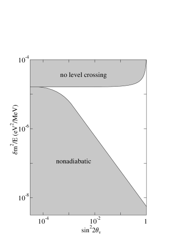
Figure 6: MSW conversion for a neutrino produced at the sun’s center. The upper shaded region indices thoses $\delta m^{2}/E$ where the vacuum mass splitting is too great to be overcome by the solar density. Thus no level crossing occurs. The lower shaded region defines the region where the level crossing is nonadiabatic ($\gamma_{c}$ less than unity). The unshaded region corresponds to adiabatic level crossings where strong $\nu_{e}\rightarrow\nu_{\mu}$ will occur.

One can envision superimposing on Fig. 6 the spectrum of solar neutrinos, plotted as a function of ${\delta m^{2}\over E}$ for some choice of $\delta m^{2}$. Since Davis sees some solar neutrinos, the solutions must correspond to the boundaries of the triangle in Fig. 6. The horizontal boundary indicates the maximum ${\delta m^{2}\over E}$ for which the sun’s central density is sufficient to cause a level crossing. If a spectrum properly straddles this boundary, we obtain a result consistent with the Homestake experiment in which low energy neutrinos (large 1/E) lie above the level-crossing boundary (and thus remain $\nu_{e}$’s), but the high-energy neutrinos (small 1/E) fall within the unshaded region where strong conversion takes place. Thus such a solution would mimic nonstandard solar models in that only the ⁸B neutrino flux would be strongly suppressed. The diagonal boundary separates the adiabatic and nonadiabatic regions. If the spectrum straddles this boundary, we obtain a second solution in which low energy neutrinos lie within the conversion region, but the high-energy neutrinos (small 1/E) lie below the conversion region and are characterized by $\gamma\ll 1$ at the crossing density. (Of course, the boundary is not a sharp one, but is characterized by the Landau-Zener exponential). Such a nonadiabatic solution is quite distinctive since the flux of pp neutrinos, which is strongly constrained in the standard solar model and in any steady-state nonstandard model by the solar luminosity, would now be sharply reduced. Finally, one can imagine “hybrid” solutions where the spectrum straddles both the level-crossing (horizontal) boundary and the adiabaticity (diagonal) boundary for small $\theta$, thereby reducing the ⁷Be neutrino flux more than either the pp or ⁸B fluxes.

What are the results of a careful search for MSW solutions satisfying the Homestake, Kamiokande/SuperKamiokande, and SAGE/GALLEX constraints? One solution, corresponding to a region surrounding $\delta m^{2}\sim 6\cdot 10^{-6}$eV² and $\sin^{2}2\theta_{v}\sim 6\cdot 10^{-3}$, is the hybrid case described above. It is commonly called the small-angle solution. A second, large-angle solution exists, corresponding to $\delta m^{2}\sim 10^{-5}$eV² and $\sin^{2}2\theta_{v}\sim$ 0.6. (Variations on these solutions include oscillations to sterile neutrinos, oscillations modified by regeneration as neutrinos pass through the earth (day/night effects), and of course vacuum oscillations.) These solutions can be distinguished by their characteristic distortions of the solar neutrino spectrum. The survival probabilities $P_{\nu_{e}}^{\rm MSW}$(E) for the small- and large-angle parameters given above are shown as a function of E in Fig. 7.

Figure 7: MSW survival probabilities P(E_ν) for typical small angle and large angle solutions.

The MSW mechanism provides a natural explanation for the pattern of observed solar neutrino fluxes. While it requires profound new physics, both massive neutrinos and neutrino mixing are expected in extended models. The small-angle solution corresponds to $\delta m^{2}\sim 10^{-5}$ eV², and thus is consistent with $m_{2}\sim$ few $\cdot 10^{-3}$ eV. This is a typical $\nu_{\tau}$ mass in models where $m_{R}\sim m_{\rm{GUT}}$. This mass is also reasonably close to atmospheric neutrino values. On the other hand, if it is the $\nu_{\mu}$ participating in the oscillation, this gives $m_{R}\sim 10^{12}$ GeV and predicts a heavy $\nu_{\tau}\sim$ 10 eV. Such a mass is of great interest cosmologically as it would have consequences for supernova physics, the dark matter problem, and the formation of large-scale structure.

There are many interesting elaborations of the MSW effect not discussed here, but treated in many papers: spin-flavor oscillations induced by the solar magnetic field [25, 26] (the mass difference between $\nu^{L}_{e}$ and a sterile $\nu^{R}_{\mu}$ is compensated by the matter effects); oscillations induced by density fluctuations [27, 28, 29]; “stochastic depolarization” effects in large random magnetic fields [30]; etc. There are also interesting effects associated with three neutrinos: if the solar neutrino problem is due to MSW $\nu_{e}-\nu_{\mu}$ oscillations, one might expect a $\nu_{e}-\nu_{\tau}$ crossing at still higher densities. This has led to many interesting speculations about the role of the MSW mechanism in supernova explosions and in supernova nucleosynthesis, and about the possibility that $\nu_{e}-\nu_{\tau}$ oscillations governed by small mixing angles might be best probed using the supernova neutrino flux.

7 Other Neutrino Mass Evidence and Implications

The solar neutrino problem is not the most compelling evidence for neutrino mass. SuperKamiokande’s analysis of the ratio of muon-like to electron-like atmospheric neutrino events confirmed that a dramatic anomaly exists. The quantity studied is

$$R={(N_{\mu}/N_{e})_{DATA}\over(N_{\mu}/N_{e})_{MC}},$$ (28)

the measured ratio of muon-like to electron-like neutrino events normalized to the expected ratio, based on Monte Carlo calculations of the production and interaction of atmospheric neutrinos. The SuperKamiokande results are [31]

$$R=0.63\pm 0.03({\rm stat})\pm 0.05({\rm syst})$$ (29)

for sub-GeV events which were fully contained in the detector and

$$R=0.65\pm 0.05({\rm stat})\pm 0.08({\rm syst})$$ (30)

for fully- and partially-contained multi-GeV events. The results for $R$ are consistent among the four largest detectors used for atmospheric neutrinos (SuperK, Soudan II, IMB, Kamiokande). While this suggests neutrino oscillations, even stronger evidence for new physics comes from measurements of $R$ as a function of the zenith angle, $\Theta$, between the vertical and neutrino direction. A down-going neutrino ($\Theta\sim 0^{o}$) travels through the atmosphere above the detector (a distance of about 20 km), whereas an up-going neutrino ($\Theta\sim 180^{o}$) has traveled through the entire Earth (a distance of about 13000 km). Hence a measurement of number of neutrinos as a function of the zenith angle yields information about their numbers as a function of the distance traveled.

Figure 8: The ratio of fully contained events measured at SuperKamiokande versus reconstructed $L/E_{\nu}$. The dashed lines show the expected shape for $\nu_{\mu}\leftrightarrow\nu_{\tau}$ oscillations with $\delta m^{2}=2.2\cdot 10^{-3}$ eV² and $\sin^{2}2\theta=1$.

The zenith angle dependence of the electron and muon fluxes [31] is shown in Fig. 8, plotted as a function of the reconstructed $L/E_{\nu}$. The muon neutrino flux drops with increasing distance, while the electron neutrino flux is approximately constant. This behavior is consistent with $\nu_{\mu}\leftrightarrow\nu_{\tau}$ oscillations. Measurements of up-going muons at Kamiokande [32] and MACRO [33], produced by high energy muon neutrino interactions in the rock below the detectors, show a similar deficit.

It is often pointed out that such results provide convincing evidence because the up/down difference in R is essentially self-normalizing: only weak geomagnetic effects are expected to break the isotropy of cosmic ray interactions in the atmosphere.

Explanations of the SuperK anomaly in terms of $\nu_{\mu}\leftrightarrow\nu_{e}$ oscillations conflict with reactor oscillation limits, while the explanation $\nu_{\mu}\leftrightarrow\nu_{sterile}$ is disfavored in fits. The preferred solution is $\nu_{\mu}\leftrightarrow\nu_{\tau}$ characterized by

$$\delta m_{23}^{2}\sim(4\pm 2)\cdot 10^{-3}eV^{2}$$

$$0.8\mathrel{\hbox to0.0pt{\lower 4.0pt\hbox{\hskip 1.0pt$\sim$}\hss}\raise 1.0pt\hbox{$<$}}\sin^{2}2\theta\mathrel{\hbox to0.0pt{\lower 4.0pt\hbox{\hskip 1.0pt$\sim$}\hss}\raise 1.0pt\hbox{$<$}}1.0.$$

The best fit mixing angle is approximately maximal, an intriguing and surprising result.

One can take the the square root of the atmospheric $\delta m^{2}$ to obtain $\sim 0.06$ eV, a minimum value for a neutrino mass. This immediately establishes a lower bound on the neutrino contribution to dark matter of about 0.3% the closure density, a value not too different from the mass evident in visible stars, a remarkable result [34].

There is one other indication of neutrino mass, the positive signal for $\bar{\nu}_{\mu}\rightarrow\bar{\nu}_{e}$ oscillations seen by the LSND group in a beam-stop experiment at Los Alamos [35]. The experiment uses a 52,000 gallon tank of mineral oil and liquid scintillator, instrumented with 1220 phototubes. A neutrino event $\bar{\nu}_{e}+p\rightarrow n+e^{+}$ is detected by the coincidence of the positron and subsequent 2.2 MeV $\gamma$ ray from neutron capture, $n+p\rightarrow d+\gamma$. The signal is consistent with $\bar{\nu}_{\mu}\rightarrow\bar{\nu}_{e}$ oscillations in a narrow band that includes the ranges $\delta m^{2}\sim$ 0.2 - 2.0 eV² and $\sin^{2}2\theta\sim 0.03-0.003$. A similar experiment at the Rutherford Laboratory, KARMEN, sees no oscillations, but has lower sensitivity [36]. A recent combined analysis [37] of the two experiments lowers the confidence level of the oscillation claim, but finds a parameter region consistent with both experiments. An improved experiment at Fermilab has been approved and should yield results in 2002.

These results have some interesting implications. For example, we discussed the quadratic seesaw relation earlier, $m_{\mathrm{light}}\sim{m_{D}^{2}\over m_{R}}$. If we use the atmospheric $\delta m^{2}$ as a rough guide to the $\nu_{\tau}$ mass (or more correctly the $\nu_{3}$ mass, given the large atmospheric neutrino mixing angle), $\nu_{3}\sim 0.1$ eV, and adopt for $m_{D}$ the corresponding third-generation quark mass, $m_{D}\sim m_{top}\sim$ 180 GeV, one obtains $m_{R}\sim 0.3\cdot 10^{15}$ GeV. This is a value reasonable close to the supersymmetric grand unified scale of $\sim 10^{16}$ GeV, a startling result. It has inspired some to hope that current neutrino results are giving us our first glimpse of physics at the GUT scale.

One puzzling aspect of atmospheric, solar, and LSND neutrino results is that they require three independent $\delta m^{2}$s. That is, they do not respect the relation

$$\delta m^{2}_{21}+\delta m^{2}_{13}+\delta m^{2}_{32}=0.$$ (31)

Thus either one of more of the experiments must be attributed to some phenomenon other than neutrino oscillations, or a fourth neutrino is required. That neutrino must be sterile to avoid constraints imposed by the known width of the $Z_{0}$.

8 Outlook

The argument that the solar neutrino problem is due to neutrino oscillations is, in a sense, circumstantial: this conclusion is derived from combining several experiments, no one of which requires new particle physics. There is no direct observation of new physics analogous to the zenith angle dependence of the SuperKamiokande atmospheric results. For this reason there is great interest in a new experiment now taking data in the Creighton nickel mine in Sudbury, Ontario, 6800 feet below the surface. The Sudbury Neutrino Observatory (SNO) has a central acrylic vessel filled with one kiloton of very pure (99.92%) heavy water, surrounded by a shield of 7.5 kilotons of ordinary water. SNO can detect electron neutrinos through the charged current reaction

$$\nu_{e}+d\rightarrow p+p+e^{-}$$ (32)

The Cerenkov light from the outgoing electron is then recorded in the array of 9800 phototubes that surround SNO’s central vessel. The spectrum of produced electrons is quite hard, making reconstruction of the energy of the $\nu_{e}$ easier than in the case of neutrino-electron elastic scattering. Thus the experimenters may be able to detect distortions of the neutrino spectrum resulting from the MSW effect.

SNO will also study the neutral current reaction

$$\nu_{x}(\bar{\nu}_{x})+d\rightarrow\nu_{x}(\bar{\nu}_{x})+p+n$$ (33)

by detecting the produced neutron either through $(n,\gamma)$ reactions on salt dissolved in the heavy water or in ³He proportional counters. In this way the experimenters will obtain an integral measurement of the flux of active neutrinos, independent of flavor. Thus a neutral current signal clearly larger than the corresponding $\nu_{e}$ signal would show that heavy-flavor neutrinos comprise a portion of the solar neutrino flux, providing definite proof of new physics.

The SNO collaboration is expected to make its first announcement of results for the charged current reaction as early as summer, 2000. In future years, as the SNO neutral and charged current results become precise and as SuperKamiokande continues to amass data, the nature of the solar neutrino problem should become much clearer. The hope is that these results, in combination with other solar neutrino results (Borexino, GNO, iodine), with new atmospheric and (possibly) supernova neutrino measurements, and with precision tests of oscillations at accelerators and reactors, will allow us to completely characterize the neutrino mass matrix, providing a window on physics well beyond the standard model.

This work was supported in part by the US Department of Energy.

References

References

- [1] A more extended popular summary of the development of neutrino physics can be found in W. C. Haxton and B. Holstein, Am. J. Phys. 68, 15 (2000).
- [2] E. Fermi, Z. Phys. 88, 161 (1934).
- [3] C. L. Cowan et al., Science 124, 103 (1956).
- [4] J. N. Bahcall, S. Basu, and M. H. Pinsonneault, Phys. Lett. B 433, 1 (1998).
- [5] A. S. Brun, S. Turck-Chieze, and P. Morel, Ap. J. 506, 913 (1998) and private communication; S. Turck-Chieze and I. Lopez, Ap. J. 408, 347 (1993).
- [6] See, for example, G. Fiorentini and B. Ricci, to appear in the Proc. of Neutrino Telescopes ‘99 (Venice) (astro-ph/9905341)
- [7] R. Davis, Jr., D. S. Harmer, and K. C. Hoffman, Phys. Rev. Lett. 20, 1205 (1968).
- [8] K. Lande, talk presented at Neutrino ’98 (Takayama, Japan, June, 1998).
- [9] J. N. Abdurashitov et al., Phys. Lett. B 328, 234 (1994) and talk presented at Neutrino ’98 (Takayama, Japan, June, 1998).
- [10] P. Anselmann et al., Phys. Lett. B 285, 376 (1992); T. Kirsten, Rev. Mod. Phys. 71, 1213 (1999).
- [11] J. N. Bahcall, Neutrino Astrophysics, (Cambridge University, Cambridge, 1989).
- [12] Y. Suzuki, Nucl. Phys. B 38, 54 (1995).
- [13] Y. Suzuki, talk presented at Lepton-Photon ’99.
- [14] V. Castellani, S. Degl’Innocenti, G. Fiorentini, M. Lissia, and B. Ricci, Phys. Rev. D 50, 4749 (1994).
- [15] A. Cumming and W. C. Haxton, Phys. Rev. Lett. 77, 4286 (1996).
- [16] F. W. W. Dilke and D. O. Gough, N 240, 262 (1972).
- [17] J. N. Bahcall, M. H. Pinsonneault, S. Basu, and J. Christensen-Dalsgaard, PRL 78, 171 (1997).
- [18] R. Epstein and J. Guzik, private communication; also see V. Berezinsky, G. Fiorentini, and M. Lissia, Phys. Rev. D 60, 123002 (1999).
- [19] K. M. Heeger and R. G. H. Robertson, Prog. Part. Nucl. Phys. 40, 135 (1998) and Phys. Rev. Lett. 77, 3720 (1996).
- [20] There has been a lot of discussion about treatments that begin with a wave packet. For recent work, see M. Nauenberg, Phys. Lett. B 447, 23 (1999).
- [21] S. P. Mikheyev and A. Smirnov, Sov. J. Nucl. Phys. 42, 913 (1985); L. Wolfenstein, Phys. Rev. D 17, 2369 (1979).
- [22] H. Bethe, Phys. Rev. Lett. 56, 1305 (1986).
- [23] W. C. Haxton, Phys. Rev. Lett. 57, 1271 (1986).
- [24] S. J. Parke, Phys. Rev. Lett. 57, 1275 (1986).
- [25] C. S. Lim and W. J. Marciano, Phys. Rev. D 37, 1368 (1988).
- [26] E. Kh. Akhmedov, Sov. J. Nucl. Phys. 48, 382 (1988).
- [27] A. Schaefer and S. E. Koonin, PLB 185, 417 (1987).
- [28] P. I. Krastev and A. Yu. Smirnov, PLB 226, 341 (1989).
- [29] W. C. Haxton and W. M. Zhang, PRD 43, 2484 (1991).
- [30] F. N. Loreti, Y. Z. Qian, G. M. Fuller, and A. B. Balantekin, PRD 52, 2264 (1995); A. B. Balantekin, J. M. Fetter, and F. N. Loreti, PRD 54, 3941 (1995).
- [31] Y. Fukuda et al. (Superkamiokande collaboration), Phys. Rev. Lett. 81, 1562 (1998); Phys. Lett. B 433, 9 (1998).
- [32] S. Hatakeyama et al. (Kamiokande collaboration), Phys. Rev. Lett. 81, 2016 (1998).
- [33] M. Ambrosio et al. (MACRO collaboration), Phys. Lett. B 434, 451 (1998).
- [34] M. Turner, astro-ph/9912211.
- [35] C. Athanassopoulos et al., Phys. Rev. Lett. 81, 1774 (1998).
- [36] B. Armbruster et al., Phys. Rev. C 57, 3414 (1998).
- [37] K. Eitel, New J. Phys. 2, 1 (2000).