STAR Note SN0420 Discussing the possibility of observation of parity violation in heavy ion collisions

Abstract

It was recently argued that in heavy ion collision the parity could be broken. This Note addresses the question of possibility of the experimental detection of the effect. We discuss how parity violating effects would modify the final particle distributions and how one could construct variables sensitive to the effect, and which measurement would be the (most) conclusive. Discussing different observables we also discuss the question if the “signals” can be faked by “conventional” effects (such as anisotropic flow, etc.) and make estimates of the signals.

I Introduction

Kharzeev, Pisarski and Tytgat[1] argue that during the evolution of the hot (QGP) fireball created in heavy ion collision meta-stable parity odd bubbles can be created. Such bubbles would have a non-zero expectation value of $\langle{\bf B}\cdot{\bf E}\rangle\neq 0$, where ${\bf B}$ and ${\bf E}$ are the chromo-magnetic and chromo-electric fields. The expectation value $\langle{\bf B}\cdot{\bf E}\rangle$ is not sign definite and would take positive and negative values with equal probabilities. Originally [1] it was proposed to look for the effect by detecting the non-statistical fluctuations in the variable

$$J=\sum_{\pi^{+},\pi^{-}}\frac{\displaystyle(\vec{p}_{\pi^{+}}\times\vec{p}_{\pi^{-}})_{z}}{\displaystyle p_{\pi^{+}}p_{\pi^{-}}}.$$ (1)

Later, Gyulassy [2] proposed to use for this purpose the so-called twist tensor:

$$T_{ij}=\sum_{\pi^{+},\pi^{-}}(\vec{p}_{\pi^{+}}\times\vec{p}_{\pi^{-}})_{i}(\vec{p}_{\pi^{+}}-\vec{p}_{\pi^{-}})_{j}.$$ (2)

Other observables as well as relations between them were also discussed in [6, 7]. The purpose of the current Note is not to discuss and compare all different P- and/or CP-odd variables (though we do discuss some of them), but instead concentrate on the general approaches to the question of experimental detection of the hypothetical bubbles with parallel electric and magnetic field. This problem clearly belongs to what now is usually called Event-by-Event (EbyE) physics. The parity violating effects modify the particle distributions on the EbyE basis and we try to apply EbyE techniques to detect the signal. We also show that sometimes the effect of parity violation can be confused with other effects (having nothing to do with parity violation) such as anisotropic flow, and caution should be used analyzing different signals.

In our discussion we adopt the idea of Chikanian and Sandweiss [3], who for simplicity proposed to simulate the effect of parity odd bubbles by bubbles with parallel (real) magnetic and electric fields randomly oriented in space. Note that the real effect caused by color fields is not necessarily opposite for positive and negative pions as it is for the real electric and magnetic fields. Thus it is very important whenever possible to measure the effect separately for each particle species including baryons and anti-baryons. The observables discussed in this Note provide such a possibility.

The Note is organized as following. The discussion of the effect of parity odd bubbles on particle momentum distributions we split into two parts. The effects related to transverse field component and due to the longitudinal component are discussed separately. Then based on the picture we get, we discuss how the effect can be observed experimentally. There exist two classes of possible observables, being sensitive only to one of the fields or to the both of them. We discuss both classes. Finally we make simple statistical estimates of the signal (and background).

In our discussion we often assume that the parity odd bubble is located at midrapidity, and we consider the effect of particle distribution modification separately in the forward and backward hemispheres. In principle the bubble can be produced anywhere in rapidity, and the corresponding splitting of the entire rapidity space into two parts can be done at any rapidity point.

II Effect of the transverse field components

We start with the case of non-zero transverse component of the electric and magnetic fields. We choose the coordinate system such that the magnetic field points in the $y$ direction. The electric field would point either in the same or in the opposite direction. The effect of the fields on the particle distribution is the following. First, the magnetic field “rotates” the distribution about the $y$ axis. Fig. 1a shows qualitatively such a rotation for positively charged particles. Next, the electric field “shifts” the entire distribution along the $y$ axis either in the positive or negative direction based on the orientation of the field and charge of the particle (Fig. 1b).

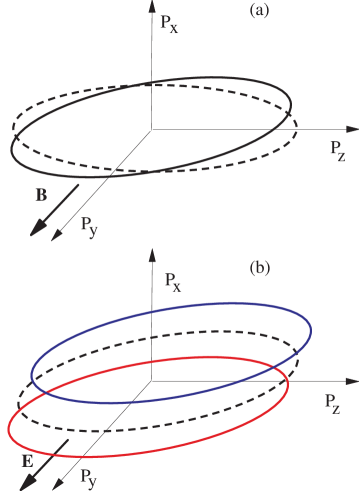
FIG. 1.: (a) The rotation of the (positive) particle distribution due to the magnetic field. (b) The shifts of the distributions of positive and negative particles in the opposite directions due to electric field.

How these changes in the distribution can be detected? The “cleanest” (and the most robust) observable for the effect would be the one which is sensitive to both fields. One of the simplest observable of this kind is the so-called $V$ variable. It is also important that this variable can be constructed using only one kind of particles (e.g. positive pions, protons, anti-nucleons, etc.). It uses the average transverse momenta of particles with positive and negative rapidities (or pseudorapidities), $\langle{\bf p}_{t}\rangle_{\eta>\eta_{c}}=(1/N_{\eta>\eta_{c}})\sum_{\eta>\eta_{c}}{\bf p}_{t}$ and $\langle{\bf p}_{t}\rangle_{\eta<\eta_{c}}=(1/N_{\eta<\eta_{c}})\sum_{\eta<\eta_{c}}{\bf p}_{t}$, where the sums run over all particles in the rapidity interval. $N_{\eta>\eta_{c}}$ and $N_{\eta<\eta_{c}}$ are the corresponding multiplicities. The result of the rotation of the distribution due to magnetic field on $\langle{\bf p}_{t}\rangle$ is opposite in the forward and backward hemispheres. Then the quantity $(\langle{\bf p}_{t}\rangle_{\eta>\eta_{c}}-\langle{\bf p}_{t}\rangle_{\eta<\eta_{c}})$ would be a good measure of the strength of the magnetic field (how it is constructed this quantity on average has nonzero “x” component, positive in Fig. 1.) (If it would be real magnetic field it could be better to weight each particle with its longitudinal momentum. We do not discuss possible weights at this moment).

The effect of the electric field is on the contrary similar in both hemispheres. To “feel” the electric field we use the quantity $(\langle{\bf p}_{t}\rangle_{\eta>\eta_{c}}+\langle{\bf p}_{t}\rangle_{\eta<\eta_{c}})$ (oriented along the “y” axis in our example if one consider positive particles). Finally we construct the variable

$$V=\{(\langle{\bf p}_{t}\rangle_{\eta>\eta_{c}}-\langle{\bf p}_{t}\rangle_{\eta<\eta_{c}})\times(\langle{\bf p}_{t}\rangle_{\eta>\eta_{c}}+\langle{\bf p}_{t}\rangle_{\eta<\eta_{c}})\}_{z}$$ (3)

The value of $V$ is directly proportional to $\langle{\bf B}\cdot{\bf E}\rangle$ and thus directly measures the effect. $V$ depends on both electric and magnetic fields and thus is quadratic in the field strengths. Due to this the effect may be small in magnitude. We leave the numeric estimates for the last section of the Note. As it was already mentioned the electric field can be either parallel or anti-parallel to the magnetic field. It means that $V$ would have both positive and negative values. The non-zero effect would manifest itself by non-statistical fluctuations in $V$. It could be measured, for example, by the sub-event method (see section on estimates and [8] for description of the method).

If the strength of the signal permits the best would be to correlate the magnitude of $(\langle{\bf p}_{t}\rangle_{\eta>\eta_{c}}+\langle{\bf p}_{t}\rangle_{\eta<\eta_{c}})$ to the perpendicular to it component of $(\langle{\bf p}_{t}\rangle_{\eta>\eta_{c}}-\langle{\bf p}_{t}\rangle_{\eta<\eta_{c}})$ in order to prove that ${\bf B}$ and ${\bf E}$ fields are correlated, or check that the electric and magnetic fields are indeed aligned, that is to check if $(\langle{\bf p}_{t}\rangle_{\eta>\eta_{c}}+\langle{\bf p}_{t}\rangle_{\eta<\eta_{c}})$ is perpendicular to $(\langle{\bf p}_{t}\rangle_{\eta>\eta_{c}}-\langle{\bf p}_{t}\rangle_{\eta<\eta_{c}})$.

Let us now discuss the possibility to observe the first order effects, namely the effects due to only magnetic or only electric field. We start with magnetic field. As can be seen directly from Fig. 1 the effect of the magnetic field (rotation about the $y$ axis and predominant particle emission in one of the transverse directions for particles in the forward hemisphere and in the opposite direction in the backward hemisphere) is indistinguishable from the effect of directed flow (which can be small but not negligible even for very central collisions). One can argue that the parity violation effect should be different for positive and negative pions, but the same could be true for directed flow. Taking into account that the effect of P/CP-odd bubbles expected to be rather small (some estimates are given below) it would be extremely difficult to disentangle it from the effect of “conventional” directed flow. Even if the effect is large one wold have to prove that the observed effect is due to the parity violation and not to anomalously large directed flow.

At this point one can ask why the effects are so similar, while directed flow obviously does not violate parity. The answer to this question is that the directed flow can “rotate” the distribution only in the reaction plane. Any rotation in any other plane would constitute the parity violation. Unfortunately, in reality we do not know the real reaction plane orientation, and the particle azimuthal distribution itself is used to determine the plane. Then it is not at all clear what is the cause for the observed anisotropy in the azimuthal particle distribution. The variable $V$ discussed above (as any other variable sensitive to both fields, e.g. the twist tensor) correlates the effects due to magnetic and electric fields and thus is not confused by the anisotropic flow.

The effect of the electric field (shifts of the positive and negative pion distributions in opposite directions) in principle should be also possible to observe, but once more one has to prove that is not due to Coulomb interactions, and/or resonance decays, etc..

III Longitudinal field components

Now we move on to the discussion of the effect of the longitudinal components of the electric and magnetic fields. The electric field “shifts” positive particles along the $z$ axis (read, rapidity) while shifting negative particles in the opposite direction. The magnetic field would “rotate” the particle distribution about the $z$ axis. In principle the magnitude of the “shift” due to the electric field could be correlated with the change in particle distribution due to magnetic field (the correlation similar to the one discussed in the previous section), but as it is shown below the effect of magnetic field itself would be an unambiguous signal of parity violation. Thus we concentrate in this section on the effects sensitive to only electric or magnetic field.

The electric field effect (relative shift of the rapidity distribution of positive and negative particles) from our point of view can be confused with the effects due to Coulomb interactions and/or resonance decays, unless the electric field effect happen to be extremely strong. The hope here would be to observe strong EbyE fluctuations in the shift, but once more one would have to calculate the possible fluctuations in Coulomb fields. Much “cleaner” signal could be the one based on the effect of the magnetic field, which presumably “rotates” the initial distribution about the $z$ axis in opposite directions for positive and negative particles. If the initial distribution is azimuthally symmetric such a rotation obviously do not produce any noticeable effect and is not detectable (as was already noticed in [3]). But in the real collisions the distribution is not expected to be azimuthally symmetric due to directed and/or elliptic flow! Then the magnetic field effect becomes observable.

The direction of the rotation of the distribution is different for positive and negative particles as shown in Fig. 2.

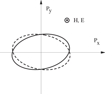
FIG. 2.: The rotation of the distribution due to longitudinal component of the magnetic field. Positive and negative particles exhibit opposite effect.

Such rotations would lead to the difference in the reaction planes reconstructed separately using positive or negative particles. One should have in mind that the final observable effect is a product of two, the anisotropic flow and the parity violation (magnetic field), and can be small. Expressed as the mean sine of the azimuthal angle difference between positive and negative particles in a given event the effect is

$$\langle\sin(\phi_{\pi^{+}}-\phi_{\pi^{-}})\rangle\approx 2v_{n}\langle\Delta\phi_{H}\rangle,$$ (4)

where $v_{n}$ ($n=1,2$) is the anisotropic flow parameter (n-th Fourier coefficient in the particle azimuthal angle distribution with respect to the reaction plane; for definition see, for example, [9]) and $\langle\Delta\phi_{H}\rangle$ is the mean (over all particles in a given event) rotation angle due to the magnetic field. $\langle\Delta\phi_{H}\rangle$ can be positive or negative depending on the orientation of the field and thus one has to study the non-statistical fluctuations in this quantity, $\sigma_{\sin(\Delta\phi),non-stat}$.

In the analysis, especially if one studies elliptic flow, it could be more convenient to use the reconstructed reaction planes, not the azimuthal angles of the individual particles. Then for a weak signal one gets:

$$\langle\sin(\Psi_{RP,\pi^{+}}-\Psi_{RP,\pi^{-}})\rangle$$ (5)

$$\approx\sqrt{N_{\pi^{+}}N_{\pi^{-}}}\langle\sin(\phi_{\pi^{+}}-\phi_{\pi^{-}})\rangle.$$ (6)

Such kind of analysis was done by the NA49 Collaboration [4, 5] for Pb+Pb collisions at CERN SPS energies. In that analysis the non-statistical fluctuations in the azimuthal angle between positive and negative pions have been measured. The results are presented as an upper limit on $\sigma_{\sin(\Delta\phi),non-stat}<10^{-3}$, the variance of the angle difference. According to the discussion above, one has to divide this quantity by the flow signal (in that case $v_{1}$) typically of a few percent in order to get the limit on the rotational angle due to the bubble magnetic field.

IV Numeric estimates

The impulse that acts on the particle crossing the bubble is estimated [10] to be about 30 MeV. It is similar for both electric and magnetic fields. Not all particles in the collision cross the bubble boundaries. The fraction would obviously depends on the bubble volume. In our estimates we will use that the mean impulse due to either field is $\Delta p\approx\alpha\cdot 30$ MeV. Then $\alpha$ would be the fraction of all particles (in the acceptance) suffered a collision with the bubble boundary. In the STAR acceptance for central Au+Au collision we expect about 2000 charged particles. In our analysis one often has to subdivide this number into two parts (e.q. forward and backward hemispheres), which gives about 1000 particles in each part. We also use an estimate (comes from RQMD) for $\langle p_{x}^{2}\rangle\approx(350~{}MeV)^{2}$. Then the “signal to background” ratio in a quantity like $\langle p_{x}\rangle_{\eta>\eta_{c}}$ would be of the order of $(\alpha\cdot 30/\sqrt{3})/(350/\sqrt{1000})\approx 1.5\alpha$, where we divided the impulse by a factor of $\sqrt{3}$, taking into account that the direction of the corresponding field is not fixed.

All quantities discussed as a signal of parity violation are not sign definite and one has look for non-statistical fluctuations in such quantities. The subevent method is probably one of the best for this purpose. This technique involves the subdivision of all particles in a given event into two groups with subsequent correlation of the signals in each of the groups (called subevents). The number of particles in a subevent is about half of that of the event, and signal to background ratio would drop to $S/B\approx\alpha$. Having in mind that one needs to correlate the subevents we get in the correlation function $S/B\approx\alpha^{2}$. The last step in this direction would be to take into account the event statistics. Then $S/B\approx\alpha^{2}\sqrt{N_{events}}$.

The above estimates are relevant mostly for a variables such as $V$ variable. For the correlation of the reaction planes the relevant quantity would be

$$\langle\theta_{H}\rangle\approx\Delta p/\sqrt{3}/\langle p_{t}\rangle\approx\alpha\cdot 30/\sqrt{3}/(\sqrt{2}\cdot 350)\approx 0.05\alpha.$$ (7)

The anisotropic flow parameters are (at SPS) of the order of $v_{n}\approx 0.02-0.06$. Then for $\sigma_{\sin(\Delta\phi),non-stat}$ one would expect values about

$$\sigma_{\sin(\Delta\phi),non-stat}\approx\alpha\cdot(1-3)\cdot 10^{-3}.$$ (8)

Remind you that the NA49 preliminary limit on this quantity is $<10^{-3}$.

V Conclusion

Parity violation in strong interactions is a question of a fundamental value. The experimental detection of the effect is a challenge and a perfect example of a problem of Event-by-Event physics. The search is expected to be difficult, but as discussed in this Note as well as in [3, 7] it is not hopeless in a sense that results valuable for theory can be obtained.

We should probably also mention here a “homework” for theorists. In the case the effect would be experimentally observed one would have to prove that it is not due to large fluctuations of the real electric and magnetic fields. Theoretical estimates of such fluctuations in the volume of the fireball created in heavy ion collision are highly desirable.

REFERENCES

- [1] D. Kharzeev, R.D. Pisarski, and M.H.G. Tytgat, Phys. Rev. Lett., 81 (1998) 512.
- [2] M. Gyulassy, RBRC MEMO 3/11/99.
- [3] A. Chikanian and J. Sandweiss, Parity and Time reversal studies in STAR, July, 1999,
- [4] S. Voloshin and the NA49 Collaboration, Search for parity violation in minimum bias Pb-Pb collisions at SPS, LBNL 1998 annual report, http://ie.lbl.gov/nsd1999/rnc/RNC.htm, report R10.
- [5] F. Sikler for the NA49 Collaboration, talk at Quark Matter ’99; http://www.qm99.to.infn.it/program/qmprogram.html
- [6] D. Kharzeev and R.D. Pisarski, preprint hep-ph/9906401.
- [7] Jim Thomas and Ron Longacre, Pattern recognition in Parity and CP Violation Studies at RHIC, LBNL 1999 annual report; Ron Longacre and Jim Thomas, Detecting CP Violation in a Left-Right Symmetric World, ibid..
- [8] S.A. Voloshin, V. Koch, and H.G. Ritter, Phys. Rev. C 60 (1999) 024901.
- [9] A.M. Poskanzer and S.A. Voloshin, Phys. Rev. C 58 (1998) 1671.
- [10] see [7] with the corresponding reference to private communication with D. Kharzeev.