Proton-Proton Fusion in Effective Field Theory

Xinwei Kong

TRIUMF, 4004 Wesbrook Mall, Vancouver, B.C., Canada V6T 2A3.

Finn Ravndal

Institute of Physics, University of Oslo, N-0316 Oslo, Norway.

Abstract: The rate for the fusion process $p+p\rightarrow d+e^{+}+\nu_{e}$ is calculated using non-relativistic effective field theory. Including the four-nucleon derivative interaction, results are obtained in next-to-leading order in the momentum expansion. This reproduces the effects of the effective range parameter. Coulomb interactions between the incoming protons are included non-perturbatively in a systematic way. The resulting fusion rate is independent of specific models and wavefunctions for the interacting nucleons. At this order in the effective Lagrangian there is an unknown counterterm which limits the numerical accuracy of the calculated rate given by the squared reduced matrix element $\Lambda^{2}(0)=7.37$. Assuming the counterterm to have a natural magnitude, we estimate the accuracy of this result to be 6% - 8%. This is consistent with previous nuclear physics calculations based on effective range theory and inclusion of axial two-body weak currents. The true magnitude of the counterterm can be determined from a precise measurement of the cross-section for low-energy neutrino scattering on deuterons.

1 Introduction

One of the most important problems in modern physics is the nature and properties of neutrinos. These were for a long time thought to be massless and stable, but experiments during the last decade have consistently shown this to be incompatible with the observed neutrino oscillations[1]. Historically and even today the fusion processes in the Sun are among the few available and abundant sources of low-energy neutrinos available for experimental investigations. In order to study oscillations in the detected fluxes, one needs to be sure of the production rates in the different nuclear reactions taking place in the Sun.

The basic process is proton-proton fusion $p+p\rightarrow d+e^{+}+\nu_{e}$. It was explained more than sixty years ago by Bethe and Critchfield when nuclear physics was still at a very primitive stage[2]. When the field had matured, it was reconsidered in the light of more modern developments by Salpeter who included effective range corrections[3]. Applications to the specific conditions we have in the Sun were investigated by Bahcall and May[4]. This work was later extended by Kamionkowski and Bahcall who also included the effects of vacuum polarization in the Coulomb interaction between the incoming protons[5]. In spite of the enormous progress in nuclear physics during this time, the methods and approximations made in these different calculations were essentially the same with a resulting accuracy in the fusion rate of a few percent. Including strong corrections due to mesonic currents at smaller scales, the uncertainty in the rate is now around one percent[6]. This is very impressive for a strongly interacting process at low energies where ordinary perturbation theory cannot be used.

In the light of the importance this fundamental process plays in connection with the solar neutrino production and possible neutrino oscillations, it is natural to reconsider the process from the point of view of modern quantum field theory instead of the old potential models used previously. A first attempt in this direction was made by Ivanov et al.[7]. In their relativistic model they obtained a result which was significantly different from the standard result based upon conventional nuclear physics models. Subsequently it was pointed out by Bahcall and Kamionowski that their effective nuclear interaction was not consistent with what is known about proton-proton scattering at low energies where Coulomb effects are important[8]. In a more recent contribution this defect of their calculation was removed and better agreement with standard results have been obtained[9].

The approach of Ivanov et al. is based upon relativistic field theory and should in principle yield reliable results. But it is well known that it is very difficult to use consistently a relativistic formulation for bound states like the deuteron. In addition, the fusion process considered here takes place at low energies and should therefore instead be described within a non-relativistic framework. Then all the large-momentum degrees of freedom are integrated out and one is left with an effective theory involving only the physically important field variables. The underlying, relativistic interactions are replaced by non-renormalizable local interactions with coupling constants which must be determined from experiments at low energies. Along these lines the proton-proton fusion rate has been calculated by Park, Kubodera, Min and Rho using chiral perturbation theory in the low-energy limit[10]. They obtain results in very good agreement with previous nuclear physics calculations. This is to be expected since they make use of phenomenological nucleon wavefunctions which fit low-energy scattering data very well. The drawback is that the results cannot be derived in an entirely analytical way.

A more fundamental approach to nucleon-nucleon interactions at low energies has been formulated by Kaplan, Savage and Wise in terms of an effective theory for non-relativistic nucleons[11][12]. It involves a few basic coupling constants which have been determined from nucleon scattering data at low energies. With no more free parameters to fit it can then be used to make predictions for a large number of other experimentally accessible quantities[13]. The effects of pions can be included using the established counting rules and higher order corrections can be derived in a systematic way. When the energy is sufficiently low as for the fusion process considered here, the effects of pions can be integrated out and absorbed into the coupling constants of the contact interactions. The resulting effective field theory which is sometimes called EFT($\pi\!\!\!/)$ then involves only nucleon fields[14]. In proton-proton scattering at low energies the Coulomb repulsion has a dominant role and can naturally be incorporated into this theory[15]. As a direct result one can derive the difference between the strong scattering length which should be approximately the same as in proton-neutron scattering, and the observed one which is modified by Coulomb effects. The relation is very similar to the old result by Jackson and Blatt[16]. Corrections due to effective-range interactions can also be included but with more difficulty due to highly divergent integrals involving Coulomb wavefunctions[17].

With this understanding of low-energy proton-proton elastic scattering, one can calculate the leading order result for the fusion process $p+p\rightarrow d+e^{+}+\nu_{e}$ taking place at essential zero initial kinetic energy[18]. With the use of a non-standard representation of the Coulomb propagator, the result is in full agreement with the corresponding leading order nuclear physics result and depends only on the physical proton-proton scattering length. To next order in the effective field theory expansion, one can derive higher order corrections[19] which also have the same structure as the corresponding effective-range corrections from more standard nuclear physics[3][4]. However, at this order there appears an unknown counterterm in the effective Lagrangian which will enter as a correspondingly unknown term in the result for the fusion rate. It can be determined from other related reactions. The most promising is neutrino scattering on deuterons at low energies which has been investigated in the same effective theory by Butler and Chen[20]. When this is done, we will also have a more accurate and predictive result for the fusion rate.

In the next section we present the theoretical framework which in the following will be used to calculate the proton-proton fusion rate in next-to-leading order in the momentum expansion of the effective theory. This is done both for the proton-neutron and proton-proton sectors. A short summary of the leading order calculation is given in section 3 followed by a more detailed calculation of the next-to-leading order corrections. The derivation of the rate is completed by the inclusion of the effects of the counterterm. In the last section the obtained result is discussed and compared with what is obtained by other methods. Using a recently improved matching of the coupling constants in the proton-neutron sector[21], we obtain a final result of $\Lambda^{2}(0)=7.37$ for the squared reduced matrix element giving the fusion rate. This is to be compared with the result of $\Lambda^{2}(0)=7.08$ derived within the corresponding effective range approximation of nuclear physics. From the dependence of the result on the magnitude of the unknown counterterm, we estimate the uncertainty to be 6% - 8%. This is significantly more than in other approaches where the unknown counterterm is replaced by definite mesonic contributions with a resulting accuracy claimed to be close to 1%. In the present effective theory a corresponding accuracy can only be hoped for when the counterterm is accurately determined in some other process. Finally, in an appendix we present a new and simpler method to regularize divergent integrals involving derivatives of the Coulomb wavefunctions at the origin.

2 Theoretical framework

In the fusion reaction $p+p\rightarrow d+e^{+}+\nu_{e}$ at low energies the incoming protons are in an antisymmetric spin singlet state. The deuteron $d$ has spin $S=1$ and the process is thus a Gamow-Teller transition mediated by the weak axial current operator ${\bf A}_{-}$ which also lowers the isospin by a unit. For a given kinetic energy $E$ and relative velocty $v_{rel}$ of the protons in the initial state, the reaction cross-section is then given by the standard formula

$$\sigma(E)={G_{A}^{2}m_{e}^{5}\over 2\pi^{3}v_{rel}}\,f(E)\,|\mbox{$\langle d\!\mid$}{\bf A}_{-}\mbox{$\mid\!pp\rangle$}|^{2}$$ (1)

where the squared matrix element must be spin averaged. Here $G_{A}$ is the weak axial vector coupling constant, $m_{e}$ is the electron mass and $f(E)$ is the Fermi function resulting from the integration over the available phase space of the leptons in the final state[22]. The available energy in the process for fusion at rest is set by the neutron-proton mass difference $\Delta M=M_{n}-M_{p}$ which is 1.294 MeV and the deuteron binding energy $B$ = 2.225 MeV. This gives an energy release of $0.931$ MeV carried away by the leptons. The temperature in the core of the Sun is approximately $15\times 10^{6}$ K which corresponds to an average proton momentum around $p=1.5$  MeV and a much smaller energy. We will therefore in the following assume that the initial proton energy $E$ approaches zero. The kinetic energy of the lepton pair will be much smaller than the momentum $\gamma=\sqrt{BM}$ of the bound nucleons with reduced mass $M/2$ in the deuteron. With the above value for the binding energy it follows that $\gamma=45.7$ MeV and thus to a very good approximation one can just ignore the momentum transfer between the leptons and the nucleons.

The difficult part of calculating the fusion cross-section (1) lies in the hadronic matrix element $T_{fi}(p)=\mbox{$\langle d\!\mid$}{\bf A}_{-}\mbox{$\mid\!pp\rangle$}$ which is a function of the initial proton momentum $p=\sqrt{EM}$. Its magnitude can easily be estimated[22]. When the proton momentum goes to zero, the $pp$ wavefunction $\psi_{p}(r)$ becomes constant over the range of the deuteron. It is simply given by the the Sommerfeld factor $C_{\eta}=e^{-\pi\eta/2}|\Gamma(1+i\eta)|$ where $\eta=\alpha M/2p$ characterizes the strength of the Coulomb repulsion between the protons[23]. The probability to find the two protons at the same point is therefore

$$C_{\eta}^{2}={2\pi\eta\over e^{2\pi\eta}-1}$$ (2)

At very low energies when $\eta$ gets large, it becomes exponentially small and is the dominant effect in the fusion reaction. Similarly, in lowest order the deuteron wavefunction is simply

$$\psi_{d}(r)=\sqrt{\gamma\over 2\pi}\;{e^{-\gamma r}\over r}$$ (3)

A rough estimate for the nuclear matrix element is then

$$T_{fi}(p)=\int\!d^{3}r\,\psi_{d}(r)\psi_{p}(r)=C_{\eta}\sqrt{8\pi\over\gamma^{3}}$$ (4)

This result sets the scale for the fusion rate. It is therefore natural to define the reduced matrix element[3]

$$\Lambda(p)=\sqrt{{\gamma^{3}\over 8\pi C_{\eta}^{2}}}\,|T_{fi}(p)|$$ (5)

which contains all the interesting and important physics. It is expected to have a value of the order of one and is now the conventional way of presenting theoretical results for the fusion rate. The goal of the present paper is to calculate this number in a more model-independent way by purely analytical methods without using any other phenomenological input than the scattering lengths and effective ranges appearing in nucleon-nucleon scattering.

2.1 KSW effective field theory

During the last couple of years much progress has been made in understanding the low-energy properties of few-nucleon systems from the non-relativistic effective field theory proposed by Kaplan, Savage and Wise[11]. At these length scales the proton and neutron are considered to be structureless point particles described by a nucleon isodoublet $N^{T}=(p,n)$ Schrödinger field. For energies well below the pion mass $m_{\pi}$, all interactions including those due to pion exchanges, will be local. In the effective Lagrangian they can be thus represented by terms involving only the nucleon field and derivatives thereof in such a way that all the symmetries obeyed by the strong interactions are preserved. At the lowest energies only $S$-waves will contribute. Including no more than terms of dimension eight in the derivative expansion, there are only two possible interaction terms in the Lagrangian parametrized by the coupling constants $C_{0}$ and $C_{2}$. It can be written as

$${\cal L}_{0} = N^{\dagger}\left(i\partial_{t}+{\nabla^{2}\over 2M}\right)N-C_{0}(N^{T}{\mbox{\boldmath$\Pi$}}N)\cdot(N^{T}{\mbox{\boldmath$\Pi$}}N)^{\dagger}$$ (6)

$$+ {1\over 2}C_{2}\left\{(N^{T}{\overrightarrow{\nabla}}\!\!\!\!\!\!{\overleftarrow{\nabla}}^{2}{\mbox{\boldmath$\Pi$}}N)\cdot(N^{T}{\mbox{\boldmath$\Pi$}}N)^{\dagger}+h.c.\right\}$$

where the operator ${\overrightarrow{\nabla}}\!\!\!\!\!\!{\overleftarrow{\nabla}}=(\overrightarrow{\nabla}-\overleftarrow{\nabla})/2$. The projection operators $\Pi_{i}$ enforce the correct spin and isospin quantum numbers in the channels under investigation. More specifically, for spin-singlet interactions $\Pi_{i}=\sigma_{2}\tau_{2}\tau_{i}/\sqrt{8}$ while for spin-triplet interactions $\Pi_{i}=\sigma_{2}\sigma_{i}\tau_{2}/\sqrt{8}$. This theory is now valid below an upper momentum $\Lambda$ which will be the physical cutoff when the theory is regularized that way. Since the pion field is integrated out, all its effects are soaked up in the two coupling constants $C_{0}$ and $C_{2}$. Then the value of the cutoff $\Lambda$ will be set by the pion mass $m_{\pi}$. In this momentum range all the main properties of few-nucleon systems are now in principle given by the above Lagrangian. More accurate results will follow from higher order operators in this field-theoretic description[14].

The effective Lagrangian (6) is non-renormalizable and divergent loop integrals must be regularized. For this purpose one can use the OS scheme of Mehen and Stewart[24] which is a generalization of the original proposal by Gegelia[25]. An equivalent method is the PDS scheme which was invented by Kaplan, Savage and Wise[11][12] and is based on dimensional regularization. We will use it here. The a priori unknown coupling constants $C_{0}$ and $C_{2}$ can be determined in terms of experimental quantities measured in low-energy nuclear reactions. The size of the dimension-six coupling constant $C_{0}$ will then be determined by the scattering length $a$ in nucleon-nucleon scattering while $C_{2}$ is found to be proportional to the effective range parameter $r_{0}$. Both of these coupling constants will depend on the renormalization mass $\mu$ which enters in the PDS regularization scheme. It can be chosen freely in the interval $\gamma<\mu\leq m_{\pi}$ but physical results obtained from the effctive theory should be independent of its precise value.

2.2 Proton-neutron interactions and the deuteron

The deuteron will appear as a bound state in proton-neutron scattering in the spin-triplet channel. It is then natural to determine the corresponding coupling constants by matching the results to properties at the deuteron pole of the scattering amplitude. The residue at the pole gives the renormalization constant $Z$ of the deuteron interpolating field which replaces the wavefunction of the bound state[12].

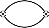
Figure 1: Feynman diagram representing the leading order contribution to the deuteron wavefunction renormalization. The crosses represent the coupling to the interpolating field for the deuteron while the lines are nucleon propagators.

In lowest order of perturbation theory one finds the renormalization constant from the irreducible 2-point function $\Sigma(E)$ shown in Fig. 1. At the two vertices the interpolating field acts with energy $E$ and zero momentum and a strength which we choose to be $-1$. In the intermediate state there is a neutron and a proton which propagate with relative momentum ${\bf k}$. Integrating over all these momenta we then find the value of the diagram,

$$\Sigma_{0}(E)=\int\!{d^{3}k\over(2\pi)^{3}}{1\over E-{\bf k}^{2}/M+i\epsilon}$$

This divergent integral is now made finite using the PDS regularization scheme[11] and gives

$$\Sigma_{0}(E)=-{M\over 4\pi}\left(\mu-\sqrt{-ME}\right)$$ (7)

The renormalization constant

$$Z=\sqrt{1\over|d\Sigma/dE|}_{E=-B}$$ (8)

which is evaluated at the deuteron pole where the binding energy is $B=\gamma^{2}/M$, thus takes the value $Z_{0}=\sqrt{8\pi\gamma}/M$ at this order of perturbation theory. It is independent of the coupling constant $C_{0}^{d}$ whose effect must be summed to all orders in order to find the non-perturbatively bound state in this channel. When it takes the special renormalized value

$$C_{0}^{d}(\mu)={4\pi\over M}{1\over\gamma-\mu}$$ (9)

we see that the reducible chain of bubble interactions in Fig. 2 just gives the same result as for the single bubble in the irreducible diagram in Fig. 1.

Figure 2: Chain of proton-neutron interactions mediated by the leading order contact term.

In this particular channel one shall therefore not sum such chains of bubble diagrams when one describes the bound state deuteron by an interpolating quantum field.

While the coupling constant $C_{0}^{d}$ must be treated non-perturbatively, the effects of the derivative coupling $C_{2}^{d}$ are included only to first order. The corresponding renormalized coupling constant is found to be $C_{2}^{d}(\mu)=\rho_{d}M(C_{0}^{d}(\mu))^{2}/8\pi$ where $\rho_{d}=1.76$ fm is the spin-triplet $pn$ effective range scattering parameter evaluated at the deuteron pole[12][14]. It will also contribute to the renormalization constant $Z$ via the perturbative diagram in Fig. 3 for the 2-point function. It has the value $\Sigma_{2}(E)=C_{2}^{d}ME\Sigma_{0}^{2}(E)$ which gives the total contribution

$$Z_{2}=Z_{0}\left[1-{\gamma M\over 2\pi}C_{2}^{d}(\mu-\gamma)(\mu-2\gamma)\right]^{-1/2}$$ (10)

In the limit $\mu\gg\gamma$ the dependence on the regularization mass $\mu$ is seen to go away. The previous value $Z_{0}$ then gets modified by the factor $\sqrt{Z_{d}}=1/\sqrt{1-\gamma\rho_{d}}$. This corresponds to a change of the normalization of the deuteron wavefunction (3) which now becomes $\psi_{d}(r)\rightarrow\sqrt{Z_{d}}\psi_{d}(r)$ in agreement with effective range theory in nuclear physics[26].

Figure 3: Effective-range correction to the deuteron wavefunction renormalization constant.

Here it is only valid at large distances since properties of the deuteron at scales less than $1/m_{\pi}$ are not accessible in this theory. Also, it is strictly only valid to first order in an expansion in powers of $\gamma\rho_{d}$ since it is obtained perturbatively in the coupling constant $C_{2}^{d}$. Since the expansion parameter has the rather large value $\gamma\rho_{d}=0.41$, it is desirable to improve the convergence of perturbation theory in this coupling constant. This has recently been achieved by Phillips, Rupak and Savage[21] whose method we will apply at the end of the more conventional approach we present first.

2.3 Coulomb interactions and the proton-proton wavefunction

In the absence of strong interactions, the incoming proton-proton state with center-of-mass momentum ${\bf p}$ is given by the Coulomb wavefunction[27]

$$\psi_{\bf p}({\bf r})={1\over\rho}\sum_{\ell=0}^{\infty}(2\ell+1)i^{\ell}e^{i\sigma_{\ell}}F_{\ell}(\rho)P_{\ell}(\cos(\theta)$$ (11)

Here $\rho=pr$ and $\sigma_{\ell}=\arg{\Gamma(1+\ell+i\eta)}$ is the Coulomb phaseshift. At low energies only the $S$-wave will contribute. It is given in terms of the Kummer function $M(a,b;z)$ as

$$F_{0}(\rho)=C_{\eta}\rho e^{-i\rho}M(1-i\eta,2;2i\rho)$$ (12)

which is a confluent hypergeometric function.

The strong interactions between the protons can now be included using the same KSW Lagrangian (6) but now with coupling constants $C_{0}^{p}$ and $C_{2}^{p}$ which also get renormalized[17].

Figure 4: Elastic scattering due to chain of bubble diagrams with Coulomb interactions. Incoming and outgoing particles are in Coulomb eigenstates.

As in the proton-neutron channel one must again consider the coupling $C_{0}^{p}$ to all orders in perturbation theory. In this way one finds that proton-proton elastic scattering is given by the infinite sum of all chains of Coulomb-dressed bubble diagrams as shown in Fig. 4. Each bubble is given by the Coulomb propagator

$$G_{C}(E;{\bf r}^{\prime},{\bf r})=M\!\int\!{d^{3}q\over(2\pi)^{3}}{\psi_{\bf q}({\bf r}^{\prime})\psi_{\bf q}^{*}({\bf r})\over p^{2}-q^{2}+i\epsilon}$$ (13)

It satisfies the Lippmann-Schwinger equation $G_{C}=G_{0}+G_{0}V_{C}G_{C}$ where $V_{C}$ is the Coulomb potential and

$$G_{0}(E;{\bf q}^{\prime},{\bf q})={M\over p^{2}-q^{2}+i\epsilon}(2\pi)^{3}\delta({\bf q}^{\prime}-{\bf q})$$ (14)

is the free propagator in momentum space. Iterating this functional equation we see from Fig. 5 that it corresponds to the exchange of zero, one, two and more static photons. Since a single bubble in Fig. 4 corresponds to the propagation of the proton pair with energy $E=p^{2}/M$ from zero separation and back to zero separation, it has the value $J_{0}(p)=G_{C}(E;{\bf r}^{\prime}=0,{\bf r}=0)$ or

$$J_{0}(p)=M\!\int\!{d^{3}q\over(2\pi)^{3}}{2\pi\eta(q)\over e^{2\pi\eta(q)}-1}{1\over p^{2}-q^{2}+i\epsilon}$$ (15)

Figure 5: The Coulomb propagator can be represented by an infinite sum of exchanged static photons between the two charged particles.

The integral is seen to be ultraviolet divergent, but can be regularized in the PDS scheme in $d=3-\epsilon$ dimensions. When contributions from poles in $d=2$ dimensions are subtracted, one finds[15]

$$J_{0}(p)={\alpha M^{2}\over 4\pi}\left[{1\over\epsilon}+\ln{\mu\sqrt{\pi}\over\alpha M}+1-{3\over 2}C_{E}-H(\eta)\right]-{\mu M\over 4\pi}$$ (16)

Here $C_{E}=0.5772$ is Euler’s constant and the function

$$H(\eta)=\psi(i\eta)+{1\over 2i\eta}-\ln(i\eta)$$ (17)

is known to appear in these Coulomb scattering problems[16]. The divergent $1/\epsilon$ piece will be absorbed in counterterms representing electromagnetic interactions at shorter scales. This replaces the bare coupling constant $C_{0}^{p}$ with the renormalized value $C_{0}^{p}(\mu)$. It can be found by matching the calculated proton-proton scattering amplitude to the experimental one. This is usually given by the measured scattering length $a_{p}=-7.82$ fm when the proton momentum $p\rightarrow 0$. Thus one finds[15]

$${1\over C_{0}^{p}(\mu)}={M\over 4\pi a_{p}}+J_{0}(0)$$ (18)

Since the function (17) is dominated by its real part $h(\eta)=1/(12\eta^{2})+{\cal O}(\eta^{-4})$ which goes to zero when $p\rightarrow 0$, we see from the form of $J_{0}(0)$ in (16) that it is natural to introduce the $\mu$-dependent scattering length

$${1\over a(\mu)}={1\over a_{p}}+\alpha M\left[\ln{\mu\sqrt{\pi}\over\alpha M}+1-{3\over 2}C_{E}\right]$$ (19)

where $\alpha$ is the fine-structure constant. It corresponds to the Jackson-Blatt relation between the strong and Coulomb-modified proton-proton scattering lengths[16]. Then we can write

$$C_{0}^{p}(\mu)={4\pi\over M}{1\over 1/a(\mu)-\mu}$$ (20)

which is now on the same form as (9) for the bound-state case.

In next order of the momentum expansion the derivative coupling $C_{2}^{p}$ in (6) is introduced perturbatively. Again matching to low-energy proton-proton scattering, one finds $C_{2}^{p}(\mu)=\rho_{d}M(C_{0}^{p}(\mu))^{2}/8\pi$ where $\rho_{p}=2.79$ fm is the the proton-proton effective range parameter. It is not affected by Coulomb corrections to this order in the effective theory. However, the $C_{2}^{p}$ coupling gives an important contribution to the scattering length (19) which picks up an additional term $-\mu\rho_{p}/2$ in the parenthesis[17].

2.4 Gamow-Teller transition operators

The dominant weak transition matrix elements in the basic fusion rate formula (1) are due to the elementary isovector axial current operator

$${\bf A}_{-}^{(1)}=N^{\dagger}{\mbox{\boldmath$\sigma$}}\tau_{-}N$$ (21)

which converts an incoming proton into a neutron with the proper spin and isospin quantum numbers. This is the ordinary one-body interaction depicted in Fig.6a. But when we include the dimension-eight derivative operator in (6) higher dimension weak transition operators must also be considered. These were first discussed by Butler and Chen in connection with elastic and inelastic scattering of neutrinos on deuterons[20]. In our case there is only one such operator which can be written as

$${\bf A}_{-}^{(2)}=L_{1A}(N^{T}{\mbox{\boldmath$\Pi$}}N)^{\dagger}(N^{T}\Pi_{-}N)$$ (22)

where the projection operator ${\mbox{\boldmath$\Pi$}}=\sigma_{2}{\mbox{\boldmath$\sigma$}}\tau_{2}/\sqrt{8}$ acts in the spin-triplet final proton-neutron state while $\Pi_{-}=\sigma_{2}\tau_{2}\tau_{-}/\sqrt{8}$ acts on the spin-singlet proton-proton initial state. The weak axial

Figure 6: One-body interaction in (a) represents the weak axial current vertex while the two-body interaction in (b) represents the higher order axial vector counterterm.

vector coupling constant has been factored out so that the effective coupling constant is just $L_{1A}$. This new two-body operator represents weak transitions taking place at shorter length scales than considered in the effective theory and the corresponding vertex is shown in Fig.6b. Typically it represents transitions due to pion interactions and other two-body interactions. In the effective theory it will act as a counterterm which can absorb the dependence on the renormalization mass $\mu$. Its actual magnitude is presently unknown. It can be estimated from dimensional arguments combined with the renormalization group. Even better would be to determine it in some other weak process where its contribution could be isolated and measured.

3 Hadronic matrix elements

We are now in position to calculate the hadronic matrix elements $T_{fi}(p)=\mbox{$\langle d\!\mid$}{\bf A}_{-}\mbox{$\mid\!pp\rangle$}$ of the weak transition operator. The initial proton state is constructed in terms of the Coulomb wavefunctions as in the elastic scattering case. For the final state deuteron we use the interpolating field which contains a proton-neutron state with the amplitude $Z$ which is the wavefunction renormalization constant. We will initially consider only the action of the axial current operator (21). The effects of spin has been separated out and will not enter the following calculation.

3.1 Leading order result

In lowest order of the effective theory only the dimension-six operators will contribute with coupling constants $C_{0}^{d}$ and $C_{0}^{p}$ in the deuteron and proton-proton sectors respectively.

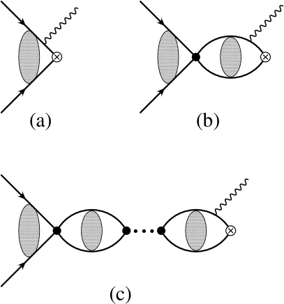
Figure 7: Feynman diagrams contributing to proton-proton fusion in leading order.

The transition matrix element $T_{fi}$ then gets contributions from three classes of diagrams shown in Fig. 7. After being hit by the weak current, the proton-proton system is transformed into a bound deuteron. The value of the simplest diagram in Fig.7a is then seen to be $Z_{0}A_{0}(p)$ where $Z_{0}$ is the constant derived in the previous section and

$$A_{0}(p)=\int\!{d^{3}k\over(2\pi)^{3}}{M\over{\bf k}^{2}+\gamma^{2}}\psi_{\bf p}({\bf k})$$ (23)

There is a factor (-1) from the deuteron vertex and the bound proton-neutron propagator is $-M/({\bf k}^{2}+\gamma^{2})$. In addition, we have introduced the Fourier transform $\psi_{\bf p}({\bf k})$ of the Coulomb wavefunction (11) when the protons have the center-of-mass momentum ${\bf p}$. Including next the strong interaction once between the two protons as shown in Fig.7b, we get the contribution $Z_{0}C_{0}B_{0}(p)\psi_{\bf p}(0)$ where

$$B_{0}(p)=\int\!{d^{3}k\over(2\pi)^{3}}{d^{3}k^{\prime}\over(2\pi)^{3}}{M\over{\bf k}^{2}+\gamma^{2}}G_{C}(E;{\bf k},{\bf k}^{\prime})$$ (24)

is a convergent integral and the last factor $\psi_{\bf p}(0)=C_{\eta}e^{i\sigma_{0}}$ gives the amplitude for the two incoming protons to meet at the first vertex. Going to higher orders in the coupling $C_{0}^{p}$ we will add in Coulomb-dressed bubble diagrams as in Fig.7c. Each bubble is of the same form as in proton-proton scattering in Fig. 4 where the contribution from each bubble is given by $J_{0}(p)$ in (15). Adding up these diagrams, they are seen to form a geometric series with the sum $C_{0}^{p}/(1-C_{0}^{p}J_{0})$. The total contribution from all the three classes of diagrams thus gives the lowest order transition amplitude $T_{fi}(p)=Z_{0}\,T_{0}(p)$ where

$$T_{0}(p)=\left[A_{0}(p)+B_{0}(p){C_{0}^{p}\psi_{\bf p}(0)\over 1-C_{0}^{p}J_{0}(p)}\right]$$ (25)

The term involving $C_{0}^{p}$ can now be expressed in terms of the proton-proton scattering length $a_{p}$ in (18) and is independent of the renormalization scale $\mu$.

For the explicit evaluation of this matrix element it is necessary to introduce the Coulomb wavefunction (12). Since the first term of the momentum integral is the product of two Fourier transformed functions, we find that it simplifies in coordinate space to

$$A_{0}(p) = MC_{\eta}e^{i\sigma_{0}}\int_{0}^{\infty}\!drre^{-(\gamma+ip)r}M(1-i\eta,2;2ipr)$$

$$= {MC_{\eta}e^{i\sigma_{0}}\over(\gamma+ip)^{2}}{{}_{2}F_{1}}\left(1-i\eta,2;2;{2ip\over\gamma+ip}\right)$$

Now the hypergeometric function ${}_{2}F_{1}(a,b,b;z)=(1-z)^{-a}$ so that the final result can be written as

$$A_{0}(p)=C_{\eta}e^{i\sigma_{0}}{M\over p^{2}+\gamma^{2}}e^{2\eta\arctan({p\over\gamma})}$$ (27)

In the expression (24) for $B_{0}(p)$ we notice that the integral over ${\bf k}^{\prime}$ gives the complex conjugate value of the Coulomb wavefunction at the origin. It therefore takes the form

$$B_{0}(p)=M\int\!{d^{3}k\over(2\pi)^{3}}\int\!{d^{3}q\over(2\pi)^{3}}{M\over{\bf k}^{2}+\gamma^{2}}{\psi_{\bf q}({\bf k})\over{\bf p}^{2}-{\bf q}^{2}+i\epsilon}\psi_{\bf q}^{*}(0)$$

The integral over ${\bf k}$ is just the previous result for $A_{0}(q)$ so that

$$B_{0}(p)=M\int\!{d^{3}q\over(2\pi)^{3}}{M\over q^{2}+\gamma^{2}}{e^{2\eta\arctan({q\over\gamma})}\over p^{2}-q^{2}+i\epsilon}{2\pi\eta(q)\over e^{2\pi\eta(q)}-1}$$ (28)

When the momentum of the incoming proton is non-zero it yields in general a complex result.

In the fusion limit $p\rightarrow 0$ we now find that the first term (27) simplifies to

$$A_{0}(p\rightarrow 0)=C_{\eta}\,{M\over\gamma^{2}}\,e^{\chi+i\sigma_{0}}$$ (29)

where the parameter $\chi=\alpha M/\gamma$. Similarly, the second term $B_{0}(p)$ becomes proportional to the integral

$$I(\chi)=\int_{0}^{\infty}\!dx{2x\over e^{x}-1}{e^{{x\over\pi}\arctan({\pi\chi\over x})}\over x^{2}+\pi^{2}\chi^{2}}$$ (30)

in the same limit when we use $x=2\pi\eta(q)$ as a new integration variable. Repeating this calculation with a different representation of the Coulomb Green’s function, it can be shown that the integral takes the value[18]

$$I(\chi)={1\over\chi}-e^{\chi}E_{1}(\chi)$$ (31)

when expressed in terms of the exponential integral

$$E_{1}(\chi)=\int_{\chi}^{\infty}dt{e^{-t}\over t}$$

With $Z_{0}=\sqrt{8\pi\gamma}/M$ for the renormalization constant, we thus find for the full matrix element the result

$$T_{fi}=\sqrt{8\pi\over\gamma^{3}}\,C_{\eta}\,e^{i\sigma_{0}}\left[e^{\chi}-\alpha Ma_{p}\,I(\chi)\right]$$ (32)

The reduced matrix element in leading order is therefore

$$\Lambda_{0}(0)=e^{\chi}-\alpha Ma_{p}\,I(\chi)$$ (33)

This is also the canonical result from standard nuclear physics[4]. The parameter $\chi=0.15$ and thus the integral $I(0.15)=4.96$. Combined with the measured value $a_{p}=-7.82$ fm for the scattering length, we then have $\Lambda_{0}(0)=2.51$ for the reduced matrix element. In the formula for the fusion rate it gives the contribution $\Lambda_{0}^{2}(0)=6.30$. From previous applications of the effective theory[13], we know that leading-order results are typically within 20 - 30% of the correct values. Going to next order in perturbation theory, the accuracy is expected to increase to 5 - 10%.

3.2 Effective range corrections

In next order of the momentum expansion of the effective field theory, there is no operator which induces $S-D$ mixing of the deuteron state. It will first appear at one order higher[12].

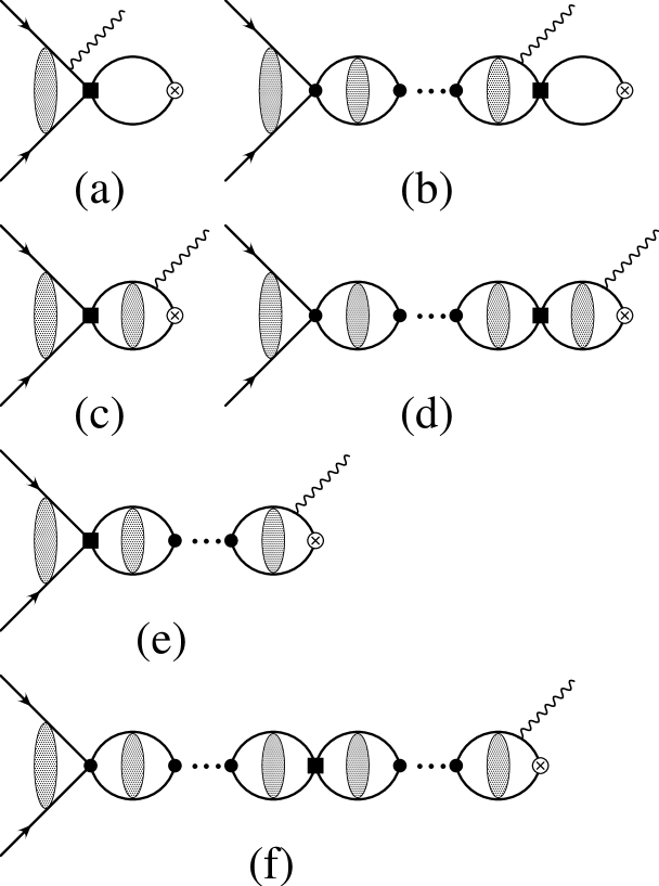
Figure 8: Corrections to the fusion amplitude coming in at next-to-leading order.

The dimension-eight couplings $C_{2}^{d}$ and $C_{2}^{p}$ give the additional diagrams shown in Fig. 8 in first order perturbation theory. Each such operator $V_{2}$ has a momentum matrix element $\mbox{$\langle{\bf k}\!\mid$}V_{2}\mbox{$\mid\!{\bf q}\rangle$}=C_{2}({\bf k}^{2}+{\bf q}^{2})/2$. The contribution from Fig.8a is seen to be

$$T_{a}={1\over 2}C_{2}^{d}\int\!{d^{3}k\over(2\pi)^{3}}\int\!{d^{3}q\over(2\pi)^{3}}{-M\over{\bf k}^{2}+\gamma^{2}}({\bf q}^{2}+{\bf k}^{2}){M\over{\bf q}^{2}+\gamma^{2}}\psi_{\bf p}({\bf q})$$ (34)

This can be expressed in terms of the divergent integral

$$I_{0}(\gamma)=-M\int\!{d^{3}k\over(2\pi)^{3}}{1\over{\bf k}^{2}+\gamma^{2}}={-M\over 4\pi}(\mu-\gamma)$$ (35)

which is the same as occured in the lowest-order determination of the wavefunction renormalization constant in (7). It is finite after PDS regularization which gives for the other occuring integral

$$I_{2}(\gamma)=-M\int\!{d^{3}k\over(2\pi)^{3}}{{\bf k}^{2}\over{\bf k}^{2}+\gamma^{2}}=-\gamma^{2}I_{0}(\gamma)$$ (36)

since $\int d^{d}k/(2\pi)^{d}=0$ in dimensional regularization. Together with the function $A_{0}(p)$ in (23) and the related function

$$A_{2}(p)=M\int\!{d^{3}k\over(2\pi)^{3}}{{\bf k}^{2}\over{\bf k}^{2}+\gamma^{2}}\psi_{\bf p}({\bf k})$$ (37)

we thus have for the matrix element (34)

$$T_{a}={1\over 2}C_{2}^{d}\left[I_{2}(\gamma)A_{0}(p)+I_{0}(\gamma)A_{2}(p)\right]$$

In the same way as we could express the integral $I_{2}(\gamma)$ in terms of $I_{0}(\gamma)$, we also find

$$A_{2}(p)=M\psi_{\bf p}(0)-\gamma^{2}A_{0}(p)$$ (38)

Here $\psi_{\bf p}(0)=C_{\eta}e^{i\sigma_{0}}$ where $\sigma_{0}$ is the Coulomb $S$-wave phaseshift. When we eventually use this result to calculate the fusion rate from (5), we will take the absolute value and this phase factor will not contribute. We therefore write

$$T_{a}={1\over 2}C_{2}^{d}I_{0}(\gamma)\left[MC_{\eta}(p)-2\gamma^{2}A_{0}(p)\right]$$

where the same phase factor also should be dropped in the last term. This result is now to be taken in the fusion limit $p\rightarrow 0$ as in the previous section.

The contribution from the diagram Fig.8b involves the Coulomb Green’s function and its derivative in the triple integral

$$T_{b1}={1\over 2}C_{2}^{d}C_{0}^{p}\int\!{d^{3}k\over(2\pi)^{3}}\int\!{d^{3}q\over(2\pi)^{3}}\int\!{d^{3}q^{\prime}\over(2\pi)^{3}}G_{C}(E;{\bf q},{\bf q}^{\prime}){M\over{\bf q}^{2}+\gamma^{2}}({\bf q}^{2}+{\bf k}^{2}){-M\over{\bf k}^{2}+\gamma^{2}}\psi_{\bf p}(0)$$

resulting from just one proton bubble. This can be expressed in terms of the function $B_{0}(p)$ in (24) and the related function

$$B_{2}(p)=M\int\!{d^{3}k\over(2\pi)^{3}}{d^{3}q\over(2\pi)^{3}}{{\bf k}^{2}\over{\bf k}^{2}+\gamma^{2}}G_{C}(E;{\bf k},{\bf q})$$ (39)

as

$$T_{b1}={1\over 2}C_{2}^{d}C_{0}^{p}[I_{2}(\gamma)B_{0}(p)+I_{0}(\gamma)B_{2}(p)]\psi_{\bf p}(0)$$

With the simplification

$$B_{2}(p)=MJ_{0}(p)-\gamma^{2}B_{0}(p)$$ (40)

we find the total contribution

$$T_{b}={1\over 2}C_{2}^{d}{I_{0}(\gamma)C_{0}^{p}\over 1-C_{0}^{p}J_{0}(p)}\left[MJ_{0}(p)-2\gamma^{2}B_{0}(p)\right]C_{\eta}$$ (41)

from all the Coulomb-dressed proton bubble diagrams in Fig.8b. Here we have again replaced $\psi_{\bf p}(0)$ by $C_{\eta}(p)$.

The remaining diagrams involve the proton derivative coupling $C_{2}^{p}$. Diagram Fig.8c gives

$$T_{c}={1\over 2}C_{2}^{p}\int\!{d^{3}q\over(2\pi)^{3}}\int\!{d^{3}k\over(2\pi)^{3}}\int\!{d^{3}k^{\prime}\over(2\pi)^{3}}{M\over{\bf k}^{\prime 2}+\gamma^{2}}G_{C}(E;{\bf k}^{\prime},{\bf k})({\bf k}^{2}+{\bf q}^{2})\psi_{\bf p}({\bf q})$$ (42)

This can again be expressed in terms of the functions $B_{0}(p)$ and $C_{\eta}(p)$ and their derivatives. In particular, we define

$$B_{2}^{\prime}(p)=M\int\!{d^{3}k\over(2\pi)^{3}}{d^{3}q\over(2\pi)^{3}}{{\bf q}^{2}\over{\bf k}^{2}+\gamma^{2}}G_{C}(E;{\bf k},{\bf q})$$ (43)

and introduce

$$\psi_{2}(p)=\int\!{d^{3}k\over(2\pi)^{3}}{\bf k}^{2}\psi_{\bf p}({\bf k})$$ (44)

which is the double derivative of the Coulomb wavefunction at the origin. Both of them are highly divergent, but can be calculated in the PDS regularization scheme and expressed in terms of already introduced functions. This is shown in the appendix. We thus find for this diagram

$$T_{c}={1\over 2}C_{2}^{p}\left[\psi_{0}(p)B_{2}^{\prime}(p)+\psi_{2}(p)B_{0}(p)\right]$$

where $\psi_{2}(p)=-\alpha M\mu\psi_{0}(p)$ in the limit $p\rightarrow 0$ as shown in the appendix. Then we also have $B_{2}^{\prime}(p)=MI_{0}(\gamma)-\alpha M\mu B_{0}(p)$ and we therefore get

$$T_{c}={1\over 2}C_{2}^{p}C_{\eta}\left[MI_{0}(\gamma)-2\alpha M\mu B_{0}(p)\right]$$ (45)

which now involves only finite and known quantities.

In Fig.8d we sum over all the Coulomb-dressed proton bubbles. The result is given by the multiple integral

$$T_{d} = {1\over 2}C_{2}^{p}{C_{0}^{p}\over 1-C_{0}^{p}J_{0}(p)}\int\!{d^{3}k\over(2\pi)^{3}}\int\!{d^{3}k^{\prime}\over(2\pi)^{3}}\int\!{d^{3}q\over(2\pi)^{3}}\int\!{d^{3}q^{\prime}\over(2\pi)^{3}}G_{C}(E;{\bf q},{\bf q}^{\prime})({\bf q}^{2}+{\bf k}^{2})$$

$$\times G_{C}(E;{\bf k}^{\prime},{\bf k}){M\over{\bf k}^{\prime 2}+\gamma^{2}}\psi_{\bf p}(0)$$

Again we can reorder the integrand so that the result is expressed in terms of simpler functions,

$$T_{d} = {1\over 2}C_{2}^{p}{C_{\eta}C_{0}^{p}\over 1-C_{0}^{p}J_{0}(p)}\left[J_{2}(p)B_{0}(p)+J_{0}(p)B_{2}^{\prime}(p)\right]$$

where now

$$J_{2}(p)=\int\!{d^{3}k\over(2\pi)^{3}}\int\!{d^{3}q\over(2\pi)^{3}}{\bf k}^{2}G_{C}(E;{\bf k},{\bf q})$$ (46)

involves the derivative of the Coulomb propagator. It is also evaluated in the appendix. In the limit $p\rightarrow 0$ we find $J_{2}(p)=-\alpha M\mu J_{0}(p)$ which together with the related result for $B_{2}^{\prime}(p)$ gives

$$T_{d}={1\over 2}C_{2}^{p}{C_{\eta}C_{0}^{p}J_{0}(p)\over 1-C_{0}^{p}J_{0}(p)}\left[MI_{0}(\gamma)-2\alpha M\mu B_{0}(p)\right]$$ (47)

It has the same structure as $T_{c}$ in (45) and they can therefore be combined into a simpler result.

The deuteron side of the diagrams in Fig.8e is seen to be just $B_{0}(p)$. Summing up the bubbles on the proton side, we find

$$T_{e}={1\over 2}{C_{2}^{p}C_{0}^{p}\over 1-C_{0}^{p}J_{0}(p)}\left[J_{2}(p)\psi_{0}(p)+J_{0}(p)\psi_{2}(p)\right]B_{0}(p)$$

In the limit $p\rightarrow 0$ this simplifies again with the result

$$T_{e}=-C_{2}^{p}C_{\eta}{C_{0}^{p}J_{0}(p)\over 1-C_{0}^{p}J_{0}(p)}\alpha M\mu B_{0}(p)$$ (48)

Similarly we find that the diagrams in Fig.8f gives

$$T_{f}={1\over 2}C_{2}^{p}\left({C_{0}^{p}\over 1-C_{0}^{p}J_{0}(p)}\right)^{2}\left[J_{2}(p)J_{0}(p)+J_{0}(p)J_{2}(p)\right]\psi_{0}(p)B_{0}(p)$$

which becomes

$$T_{f}=-C_{2}^{p}C_{\eta}\left({C_{0}^{p}J_{0}(p)\over 1-C_{0}^{p}J_{0}(p)}\right)^{2}\alpha M\mu B_{0}(p)$$ (49)

in the low-energy limit $p\rightarrow 0$.

Adding now up the contributions from all the diagrams in Fig. 8, we obtain the sum

$$T_{2} = -\gamma^{2}C_{2}^{d}I_{0}(\gamma)T_{0}(p)+{1\over 2}(C_{2}^{p}+C_{2}^{d}){MI_{0}(\gamma)C_{\eta}\over 1-C_{0}^{p}J_{0}(p)}$$

$$- {\alpha M\mu C_{2}^{p}C_{\eta}B_{0}(p)\over(1-C_{0}^{p}J_{0}(p))^{2}}$$

where $T_{0}(p)$ is the lowest order matrix element (25). The full transition matrix element to this order is therefore

$$T_{fi}=Z_{2}T_{0}(p)+Z_{0}T_{2}(p)$$

where $Z_{2}$ is the next-to-leading order renormalization constant (10). Reordering and combining terms, we obtain

$$Z_{0}^{-1}T_{fi} = A_{0}(p)+B_{0}(p)C_{\eta}\left[{C_{0}^{p}\over 1-C_{0}^{p}J_{0}(p)}-{\alpha M\mu\,C_{2}^{p}\over[1-C_{0}^{p}J_{0}(p)]^{2}}\right]$$ (50)

$$+ {\gamma M\over 4\pi}C_{2}^{d}(\mu)(\mu-\gamma)^{2}\left[A_{0}(p)+B_{0}(p){C_{\eta}C_{0}^{p}\over 1-C_{0}^{p}J_{0}(p)}\right]$$ (51)

$$- {M^{2}\over 8\pi}C_{\eta}(\mu-\gamma){C_{2}^{p}+C_{2}^{d}\over 1-C_{0}^{p}J_{0}(p)}$$ (52)

In the bubble integral $J_{0}(p)$ we can take $p\rightarrow 0$ since it is finite. The function $B_{0}(p)$ is also finite in this limit while $A_{0}(p)$ becomes proportional to the Coulomb factor $C_{\eta}(p)$ which diverges. As shown previously in the application of the same effective theory to low-energy, elastic proton-proton scattering, the first square bracket is now just the physical proton-proton scattering length $a_{p}$ calculated in next-to-leading order with the result[17]

$$a_{p}={M\over 4\pi}\left({C_{0}^{p}\over 1-C_{0}^{p}J_{0}(0)}-{\alpha M\mu\,C_{2}^{p}\over[1-C_{0}^{p}J_{0}(0)]^{2}}\right)$$ (53)

The last term is the effective-range correction which is important in order to have a physically meaningful result for the scattering length. We see that when this is zero, we have the previous result (18) used in leading order.

The transition matrix element in next-to-leading order is now given by (52). Isolating a common factor, the reduced matrix element (5) follows as

$$\Lambda_{2}(0)=\Lambda_{0}(0)\left[1+{\gamma M\over 4\pi}C_{2}^{d}(\mu)(\mu-\gamma)^{2}\right]-a_{p}\gamma^{2}(\mu-\gamma){C_{2}^{p}(\mu)+C_{2}^{d}(\mu)\over 2C_{0}^{p}(\mu)}$$ (54)

where $\Lambda_{0}(0)$ is the leading-order result (33) but now expressed in terms of the next-to-leading order scattering length (53). With the already established value for the coupling constant $C_{2}^{d}$ we see that it is now multiplied by the factor $1+\gamma\rho_{d}/2$. This can be interpreted as the first term in the expansion of the deuteron normalization factor $Z_{d}$ discussed in the previous section. While this term in the result is independent of the renormalization scale $\mu$, we see that the last term is generally not. However, when $\mu$ is much larger than the other mass scales given by the scattering lengths, this dependence goes away and we are left with the definite result

$$\Lambda_{2}(0)_{\mu\gg\gamma}=\Lambda_{0}(0)\left[1+{1\over 2}\gamma\rho_{d}\right]+{1\over 4}a_{p}\gamma^{2}(\rho_{p}+\rho_{d})$$ (55)

It has a structure which is very similar to the reduced matrix element in the standard nuclear physics effective-range approximation[3][4]

$$\Lambda_{ER}(0)=\sqrt{Z_{d}}\left[\Lambda_{0}(0)+{1\over 4}a_{p}\gamma^{2}(\rho_{p}+\rho_{d})\right]$$ (56)

With the known values for the different nucleon parameters, the result in this old approximation is therefore $\Lambda_{ER}(0)=2.66$ or $\Lambda_{ER}^{2}(0)=7.08$. On the other hand, our next-to-leading order result (55) gives $\Lambda_{2}(0)_{\mu\gg\gamma}=2.54$ which is just a 1.4% addition to the leading order result we previously obtained . This is surprisingly small, but results from an almost total cancellation between the two effective-range corrections in (55). The net result for the squared matrix element is $\Lambda_{2}^{2}(0)_{\mu\gg\gamma}=6.45$ which is seen to be 8% below the effective-range value.

3.3 Contribution from counterterm

A complete calculation of the fusion rate in next-to-leading order must include all operators contributing to this order in the momentum expansion of effective theory. Until now we have only included the effects of the dimension-eight operators coupling four nucleons with a derivative interaction. Since our result above in general depends on the renormalization scale, it signals that the calculation is incomplete. There should be additional interaction terms that in principle should absorb all dependence on the renormalization scale. This is in fact the case as shown by Butler and Chen[20] and discussed in the introductory section. It has the structure as given in (22) and corresponds to the weak current coupling directly to the four-nucleon vertex. In a more fundamental theory it could be due to weak interactions via virtual pions, coupling to excited nucleons or more general two-body operators in nuclear physics language. Obviously, this counterterm will also modify the numerical result for the fusion rate in addition to softening the $\mu$-dependence.

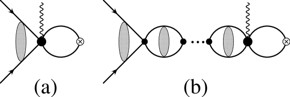
Figure 9: Contributions to the fusion amplitude from the counterterm.

In our case it gives a contribution depicted by the Feynman diagram in Fig.9a. It is similar to the previously calculated contribution from Fig.8a in (34) and becomes

$$T_{a}^{\,ct}=L_{1A}\int\!{d^{3}k\over(2\pi)^{3}}\int\!{d^{3}q\over(2\pi)^{3}}{M\over{\bf k}^{2}+\gamma^{2}}\psi_{\bf p}({\bf q})=-L_{1A}C_{\eta}I_{0}(\gamma)$$ (57)

The strong interactions in the initial state, now to lowest order in the derivative expansion, gives the series of diagrams shown in Fig.9b. They form again an infinite geometric series whose sum

$$T_{b}^{\,ct}=-L_{1A}\,C_{\eta}I_{0}(\gamma){C_{0}^{p}J_{0}(p)\over 1-C_{0}^{p}J_{0}(p)}$$ (58)

is given by the proton-proton physical scattering length $a_{p}$ from (18) and $a(\mu)$ from (20) in the fusion limit $p\rightarrow 0$. With the regularized value for the integral $I_{0}$, we thus find the total contribution from the counterterms to be

$$T^{\,ct}=-L_{1A}\,C_{\eta}{M\over 4\pi}(\mu-\gamma)\left[\mu-{1\over a(\mu)}\right]a_{p}$$ (59)

The corresponding reduced matrix element then follows from (5) after multiplication by the wavefunction renormalization constant $Z_{0}$.

We now include this new contribution as a correction to the matrix element (54) coming from the ordinary axial current interactions. For the combined result we then have

$$\Lambda_{2}^{ct}(0) = \Lambda_{0}(0)\left[1+{1\over 2}\gamma\rho_{d}\right]-{a_{p}\gamma^{2}\over 4\pi}(\mu-\gamma)\left[\mu-{1\over a(\mu)}\right]$$ (60)

$$\times \left[L_{1A}(\mu)-{M\over 2}\left(C_{2}^{p}(\mu)+C_{2}^{d}(\mu)\right)\right]$$

The coupling constant $L_{1A}$ of the counterterm must have a dependence on the renormalization scale $\mu$ so that the total $\mu$-dependence in the last term is negligible. When $\mu\gg\gamma$ we see that this requirement leads to

$$L_{1A}(\mu)_{\mu\gg\gamma}={4\pi\ell_{1A}\over M\mu^{2}}$$ (61)

where $\ell_{1A}$ is an unknown, dimensionless constant. It is set by physics on scales shorter than $1/m_{\pi}$ and its natural value should be around one as pointed out by Butler and Chen[20]. In order to get a rough idea of the sensitivity of the result on this parameter, we take $\mu=m_{\pi}$ which is the scale at which one should match the effective theory to the more fundamental theory involving pions. Varying then $\ell_{1A}$ in the interval $[-1,1]$, we find that the fusion rate measured by $\Lambda_{2}^{ct}(0)^{2}$ varies linearly from 6.22 to 6.84. These values are seen to be systematically below the effective-range result following from (56), but are within the 5% - 10% uncertainty range expected at this order.

4 Discussion and conclusion

Effective field theory is a very powerful approach to low-energy phsyics. It can hardly be said to be wrong when used correctly since it is just based upon the basic symmetries of the problem and standard quantum field theory. In that way it is a very conservative approach since it does not admit assumptions about the physics on scales shorter than it is meant to handle. Instead of such specific and model-dependent assumptions, one has higher-dimensional contact interactions and counterterms with coupling constants which represent the unknown physics. The most common criticism against effective field theory is therefore that it is not accurate enough since the results may depend on one or more such coupling constants which are not a priori known. One can make estimates of these unknown coupling constants based upon some kind of naturalness supported by dimensional analysis and the renormalization group.

But these counterterms do not really represent a weakness of effective field theory. Since they are interactions appearing in a Lagrangian, they will appear with the same strength in many different processes. If one or more of these allow for the determination of the corresponding coupling constants, one can then make much more accurate predictions for the other reactions. One recent example is radiative neutron-proton capture $n+p\rightarrow d+\gamma$. When the process takes place at very low energies or at rest, it is dominated by a magnetic dipole transition which at next-to-leading order also involves a four-nucleon counterterm very similar to the one we have considered here for proton-proton fusion. From the measured rate at these low energies, the counterterm can then be determined numerically[14]. The same neutron-proton fusion process is also a key reaction in big-bang nucleosynthesis where it takes place at energies upto around 1 MeV. Chen and Savage have now calculated the corresponding cross section with an uncertainty of 4% based on the measured counterterm[28]. A similar accuracy can be expected also for proton-proton fusion if the counterterm can be determined in some other process.

It has already been pointed out that our results for the proton-proton fusion have a very similar structure to what one finds in the effective-range approximation in nuclear physics. This has also been seen in other processes investigated within the same effective theory and at higher orders in the perturbative expansion[12][14]. It is understood when one realizes that these processes are dominated by the properties of the deuteron wavefunction at large distance scales which is contained in the effective-range approximation. In the KSW field theory, these properties are coded into the coupling constants $C_{0}^{d}$ and $C_{2}^{d}$. While $C_{0}^{d}$ is responsible for binding the deuteron and must be treated non-perturbatively, the effects of $C_{2}^{d}$ are to be treated perturbatively and gives the detailed behaviour of the wavefunction at large distances. In the above $C_{2}^{d}$ was determined by matching to the effective range parameter $\rho_{d}$. In order to get better agreement with low-energy proton-neutron scattering data which are related directly to the deuteron bound state wavefunction via analytical continuation, it has recently been pointed out by Phillips, Rupak and Savage that one should instead match $C_{2}^{d}$ to the wavefunction normalization parameter $Z_{d}$[21]. This gives the result

$$C_{2}^{d}(\mu)={2\pi\over\gamma M}{Z_{d}-1\over(\mu-\gamma)^{2}}$$ (62)

where $Z_{d}=1.69$. They have shown that this markedly improves the convergence of the perturbative calculation of many processes involving deuterons at low energies. Rupak has recently applied this improved method to neutron-proton fusion $n+p\rightarrow d+\gamma$ at energies relevant to big-bang nucleosynthesis as discussed above[29]. Including one higher order in the perturbative expansion of the elctric transition amplitude, he has then obtained an accuracy of 1% for the calculated cross section.

In our case we can now use this new value for $C_{2}^{d}$ in the result (54) for the reduced matrix element. Including also the counterterm as in (60), we then obtain our final result. Again the counterterm coupling constant will have the form (61) for large values of the renormalization mass. Choosing $\mu=m_{\pi}$, we now find that $\Lambda_{2}^{2}(0)$ varies between 7.04 and 7.70 when the parameter $\ell_{1A}$ takes values in the interval $[-1,1]$. With the size of the unknown counterterm in this range, we thus have the central value $\Lambda_{2}^{2}(0)=7.37$ with a conservative estimate for the uncertainty of 6% - 8%. We thus find a somewhat higher value for the fusion rate in this improved perturbative calculation compared with results from effective range theory (56) and the inclusion of axial two-body effects[6]. But these other results are now within the accuracy range of the effective field theory method. Should there in the future turn out to be a real discrepancy between these different theoretical descriptions, it can only be due to meson processes at shorter scales which have been overlooked or not correctly handled in the more conventional nuclear physics approach.

The only way to improve the accuracy and thus obtain a more predictive result, is to establish the value of the counterterm coupling constant $L_{1A}$. In principle it could be measured in many other reactions, but the most promising is elastic and inelastic scattering of neutrinos on deuterons as shown by Butler and Chen[20]. High-precision experimental results for these reactions would then result in a known value of the relevant counterterm. As shown by Rupak for radiative neutron capture, one should then be in the position to obtain the proton-proton fusion rate with a much improved accuracy. This will place our understanding of this fundamental process on a more solid basis. Needless to say, it will also strengthen our knowledge of the neutrino production rate in the Sun.

5 Acknowledgement

We want to thank John Bahcall, Jiunn-Wei Chen, Peter Lepage, Gautam Rupak, Martin Savage and Mark Wise for encouragement and many helpful discussions. Most of this work was done in the Department of Physics and INT at the University of Washington in Seattle and we are grateful for generous support and hospitality.

6 Appendix

We will here regularize and evaluate the divergent integrals involving Coulomb wavefunctions which are needed for the effective-range corrections to the fusion rate. Some of them have previously been encountered in connection with higher order corrections to low-energy proton-proton elastic scattering[17]. They were then calculated by a method based on regularization of the Fourier-transformed Coulomb wavefunctions. We will here use a different and simpler method.

The simplest integral is $J_{2}(p)$ in (46) which we rewrite as

$$J_{2}(p)=p^{2}J_{0}(p)+\int\!{d^{3}k\over(2\pi)^{3}}\int\!{d^{3}q\over(2\pi)^{3}}({\bf k}^{2}-{\bf p}^{2})\,\mbox{$\langle{\bf k}\!\mid$}G_{C}(E)\mbox{$\mid\!{\bf q}\rangle$}$$

It represents a Coulomb-dressed bubble propagator with a derivative interaction at one vertex. Here we have introduced the free eigen-momentum states $\langle{\bf k}\!\mid$ and $\mid\!{\bf q}\rangle$. The Coulomb propagator $G_{C}(E)$ satifies the Lippmann-Schwinger equation $G_{C}=G_{0}+G_{0}V_{C}G_{C}$ where $G_{0}(E)$ is the free propagator (14) and $V_{C}$ is the Coulomb potential. In momentum space it has the matrix element $\mbox{$\langle{\bf k}\!\mid$}V_{C}\mbox{$\mid\!{\bf k}^{\prime}\rangle$}=4\pi\alpha/({\bf k}-{\bf k}^{\prime})^{2}$. The first term will now give zero with the use of dimensional regularization,

$$\int\!{d^{d}k\over(2\pi)^{d}}=0$$ (63)

We then insert two complete sets of momentum eigenstates between the three operators in the matrix elements in the second term. The denominator in the free propagator $G_{0}$ then cancels against the factor ${\bf k}^{2}-{\bf p}^{2}$ in the integral. We are thus left with

$$\int\!{d^{3}k\over(2\pi)^{3}}({\bf k}^{2}-{\bf p}^{2})\,\mbox{$\langle{\bf k}\!\mid$}G_{0}V_{C}G_{C}\mbox{$\mid\!{\bf q}\rangle$}=-M\int\!{d^{3}k\over(2\pi)^{3}}\int\!{d^{3}k^{\prime}\over(2\pi)^{3}}{4\pi\alpha\over({\bf k}-{\bf k}^{\prime})^{2}}\mbox{$\langle{\bf k}^{\prime}\!\mid$}G_{C}(E)\mbox{$\mid\!{\bf q}\rangle$}$$

In the integral over ${\bf k}$ we now shift the integration variable ${\bf k}\rightarrow{\bf k}+{\bf k}^{\prime}$ and use the PDS regularization result

$$\int\!{d^{3}k\over(2\pi)^{3}}{4\pi\alpha\over{\bf k}^{2}}=\alpha\mu$$ (64)

The remaining two integrals over ${\bf k}^{\prime}$ and ${\bf q}$ then simply gives $J_{0}(p)$. We thus have the result

$$J_{2}(p)=[p^{2}-\alpha M\mu]\,J_{0}(p)$$ (65)

Except for a higher order term in the fine-structure constant $\alpha$, this agrees with what we obtained with the much more cumbersome wavefunction regularization method[17].

The next integral $\psi_{2}(p)$ in (44) corresponds to the double drivative of the Coulomb wavefunction at the origin. We can write it as

$$\psi_{2}(p)=p^{2}\psi_{0}(p)+\int\!{d^{3}k\over(2\pi)^{3}}({\bf k}^{2}-{\bf p}^{2})\,{\mbox{$\langle{\bf k}\,$}}\mbox{$\mid\!\psi_{\bf p}\rangle$}$$

where $\mid\!\psi_{\bf p}\rangle$ is a Coulomb state with momentum ${\bf p}$. It can formally be expressed in terms of the free state $\mid\!{\bf p}\rangle$ as

$$\mbox{$\mid\!\psi_{\bf p}\rangle$}=[1+G_{C}V_{C}]\mbox{$\mid\!{\bf p}\rangle$}$$

One then has

$$\int\!{d^{3}k\over(2\pi)^{3}}({\bf k}^{2}-{\bf p}^{2})\,{\mbox{$\langle{\bf k}\,$}}\mbox{$\mid\!\psi_{\bf p}\rangle$} = \int\!{d^{3}k\over(2\pi)^{3}}({\bf k}^{2}-{\bf p}^{2})\,\left[\mbox{$\langle{\bf k}\!\mid$}G_{0}V_{C}\mbox{$\mid\!{\bf p}\rangle$}+\mbox{$\langle{\bf k}\!\mid$}G_{0}V_{C}G_{C}V_{C}\mbox{$\mid\!{\bf p}\rangle$}\right]$$

$$= \int\!{d^{3}k\over(2\pi)^{3}}({\bf k}^{2}-{\bf p}^{2})\,\mbox{$\langle{\bf k}\!\mid$}G_{0}V_{C}\mbox{$\mid\!\psi_{\bf p}\rangle$}$$

using $G_{C}V_{C}\mbox{$\mid\!{\bf p}\rangle$}=\mbox{$\mid\!\psi_{\bf p}\rangle$}-\mbox{$\mid\!{\bf p}\rangle$}$ in the last term. Inserting now again two complete sets of free momentum states as above, it follows that

$$\psi_{2}(p)=p^{2}\psi_{0}(p)-M\int\!{d^{3}k\over(2\pi)^{3}}\int\!{d^{3}q\over(2\pi)^{3}}{4\pi\alpha\over({\bf k}-{\bf q})^{2}}{\mbox{$\langle{\bf q}\,$}}\mbox{$\mid\!\psi_{\bf p}\rangle$}$$

After a shift of integration variable, we have the result

$$\psi_{2}(p)=[p^{2}-\alpha M\mu]\,\psi_{0}(p)$$ (66)

when making use the the PDS regularized integral (64).

The last integral we need is $B_{2}^{\prime}(p)$ in (43). Rewriting it as above, it takes the form

$$B_{2}^{\prime}(p)=p^{2}B_{0}(p)+M\int\!{d^{3}k\over(2\pi)^{3}}{d^{3}q\over(2\pi)^{3}}{{\bf q}^{2}-{\bf p}^{2}\over{\bf k}^{2}+\gamma^{2}}G_{C}(E;{\bf k},{\bf q})$$

where the first term is the finite integral (24). In the second term we can use the Lippmann-Schwinger equation for the Coulomb propagator. Again we find that the denominator of the free propagator cancels against ${\bf q}^{2}-{\bf p}^{2}$ in the numerator. The first term in the integral gives then just the integral $I_{0}(p)$ in (35). Going through the same steps as above with insertion of complete sets of states, the second term is then reduced to the finite integral $B_{0}(p)$. In this way we obtain

$$B_{2}^{\prime}(p)=MI_{0}(p)+[p^{2}-\alpha M\mu]\,B_{0}(p)$$ (67)

which again is a surprising simple result.

We notice that these three divergent Coulomb integrals contain the common factor $p^{2}-\alpha M\mu$ in the results. This can be understood as coming from the divergence of the double derivative of the Coulomb wavefunction $\psi_{\bf p}({\bf r})$ at the origin. It satisfies the Schödinger wave equation

$$\left[-{1\over M}{\mbox{\boldmath$\nabla$}}^{2}+V_{C}(r)\right]\psi_{\bf p}({\bf r})=E\psi_{\bf p}({\bf r})$$

where the energy $E=p^{2}/M$. When we now take the limit $r\rightarrow 0$, it follows that

$$-{\mbox{\boldmath$\nabla$}}^{2}\psi_{\bf p}({\bf r})_{r\rightarrow 0}=[p^{2}-\alpha M\mu]\,\psi_{\bf p}(0)$$ (68)

since the regularized integral (64) is just the Coulomb potential at the origin.

References

- [1] J.N. Bahcall, Phys. Rev. D58, 096016 (1998); Neutrino Astrophysics, Cambridge University Press, Cambridge, 1989.
- [2] H.A. Bethe and C.L. Chritchfield, Phys. Rev. 54, 248 (1938).
- [3] E.E. Salpeter, Phys. Rev. 88, 547 (1952).
- [4] J.N. Bahcall and R.M. May, Ap. J. 155, 501 (1969).
- [5] M. Kamionkowski and J.N. Bahcall Ap. J. 420, 884 (1994).
- [6] R. Schiavilla, V.G.J. Stoks, W. Glöckle, H. Kamada, A. Nogga, J. Carlson, R. Machleidt, V.R. Pandharipande, R.B. Wiringa, A. Kievsky, S. Rosati and M. Viviani, Phys. Rev. C58, 1263 (1998).
- [7] A.N. Ivanov, N.I. Troitskaya, M. Faber and H. Oberhummer, Nucl. Phys. A617, 414 (1997); Errata ibid. A618, 509 and A625 896; H. Oberhummer, A.N. Ivanov, N.I. Troitskaya and M. Faber, astro-ph/9705119.
- [8] J.N. Bahcall and M. Kamionkowski, Nucl. Phys. A625, 893 (1997).
- [9] A.N. Ivanov, H. Oberhummer, N.I. Troitskaya and M. Faber, nucl-th/9910021.
- [10] T.-S. Park, K. Kubodera, D.-P. Min and M. Rho, Ap. J. 507, 443 (1998).
- [11] D.B. Kaplan, M.J. Savage and M.B. Wise, Phys. Lett. B424, 390 (1998); Nucl. Phys. B534, 329 (1998).
- [12] D.B. Kaplan, M.J. Savage and M.B. Wise, Phys. Rev. C59, 617 (1999).
- [13] P.F. Bedaque, M.J. Savage, R. Seki and U. van Kolck (editors), Nuclear Physics with Effective Field Theory II, World Scientific, Singapore, 2000.
- [14] J.-W. Chen, G. Rupak and M.J. Savage, Nucl. Phys. A653, 386 (1999).
- [15] X. Kong and F. Ravndal, Phys. Lett. B450, 320 (1999).
- [16] J.D. Jackson and J.M. Blatt, Rev. Mod. Phys. 22, 77 (1950).
- [17] X. Kong and F. Ravndal, Nucl. Phys. A665, 137 (2000).
- [18] X. Kong and F. Ravndal, Nucl. Phys. A656, 421 (1999).
- [19] X. Kong and F. Ravndal, Phys. Lett. B470, 1 (1999).
- [20] M. Butler and J.-W. Chen, nucl-th/9905059.
- [21] D.R. Phillips, G. Rupak and M.J. Savage, nucl-th/9908054.
- [22] M.G. Bowler, Nuclear Physics, Pergamon Press, London, 1973.
- [23] A. Sommerfeld, Atombau und Spektrallinien, Vol. II, Vieweg, Braunschweig, 1939; L.D. Landau and E.M. Lifschitz, Quantum Mechanics, Pergamon Press, London, 1958.
- [24] T. Mehen and I.W. Stewart, Phys. Lett. B445, 378 (1999); Phys. Rev. C59, 2365 (1999).
- [25] J. Gegelia, Phys. Lett. B429, 227 (1998).
- [26] H.A. Bethe, Phys. Rev. 76, 38 (1949).
- [27] M. Abramowitz and I.A. Stegun, Handbook of Mathematical Functions, Dover Publications, Inc., New York, 1972.
- [28] J.-W. Chen and M. Savage, nucl-th/9907042.
- [29] G. Rupak, nucl-th/9911018.