Nuclear structure from random interactions
Abstract
Low-lying states in nuclei are investigated using an ensemble of random interactions. Both in the nuclear shell model and in the interacting boson model we find a dominance of ground states. It is shown that this feature is not due to time reversal symmetry. In the shell model, evidence is found for the occurrence of pairing properties, and in the interacting boson model for both vibrational and rotational band structures. Our results suggest that these features represent general and robust properties of the model space, and do not depend on details of the interactions.
pacs:
PACS numbers: 21.60.Cs, 21.60.Ev, 21.60.Fw, 24.60.LzI Introduction
Despite the fact that nuclei are complex many-body systems with many degrees of freedom, their spectral properties often show very regular features. A recent analysis of experimental energy systematics of medium and heavy even-even nuclei suggests a tripartite classification of nuclear structure into seniority, anharmonic vibrator and rotor regions [1, 2]. Plots of the excitation energies of the yrast states with against show a characteristic slope for each region: 1.00, 2.00 and 3.33, respectively. In each of these three regimes, the energy systematics is extremely robust. Moreover, the transitions between different regions occur very rapidly, typically with the addition or removal of only one or two pairs of nucleons. The transition between the seniority region (either semimagic or nearly semimagic nuclei) and the anharmonic vibrator regime (either vibrational or soft nuclei) was addressed in a simple schematic shell model calculation and attributed to the proton-neutron interaction [3]. The empirical characteristics of the collective regime which consists of the anharmonic vibrator and the rotor regions, as well as the transition between them, have been studied [4, 5] in the framework of the interacting boson model (IBM) [6]. An analysis of phase transitions in the IBM [7, 8] has shown that the collective region is characterized by two basic phases (spherical and deformed) with a sharp transition region [9, 10], rather than a gradual softening which is traditionally associated with the onset of deformation in nuclei.
In a separate development, the characteristics of low-energy spectra of many-body even-even nuclear systems have been studied recently in the context of the nuclear shell model (SM) with random two-body interactions [11, 12]. Despite the random nature of the interactions, the low-lying spectra still show surprisingly regular features, such as a predominance of ground states separated by an energy gap from the excited states. This is contrary to the traditional wisdom in which the favoring of ground states is attributed to the nuclear pairing arising from the short-range nuclear force. A subsequent analysis of the pair transfer amplitudes has shown that pairing is a robust feature of the general two-body nature of shell model interactions and the structure of the model space [13]. On the other hand, no evidence was found for rotational band structures.
The existence of robust features in the low-lying spectra of medium and heavy even-even nuclei [1, 2] suggests an underlying simplicity of low-energy nuclear structure never before appreciated. In order to address this point we carry out a study of the systematics of energy levels in the framework of the SM and the IBM with random interactions. We address time-reversal symmetry in connection with the dominance of ground states, look for regular spectral properties, and investigate the effect of many-body interactions.
II The nuclear shell model
We first consider the properties of nuclei in the presence of random interactions within the context of the shell model. As a model space we take that of identical nucleons in the shell, which consists of single-particle orbitals with , 3/2 and 5/2 . The case of particles is one of the examples considered in [11, 12] and referred to as corresponding to the nucleus 22O. For identical particles the isospin is the same for all states, and hence does not play a role. In Ref. [12] it was shown that the single-particle energies have little effect on the results, and therefore they are not considered here. The two-body interactions can be expressed as
| (1) |
with
| (2) | |||||
| (3) | |||||
| (4) | |||||
| (5) | |||||
| (6) | |||||
| (7) | |||||
| (8) | |||||
| (9) | |||||
| (10) | |||||
| (11) | |||||
| (12) | |||||
| (13) | |||||
| (14) | |||||
| (15) |
The coefficients correspond to the 30 two-body matrix elements for identical particles in the shell. They are chosen independently from a Gaussian distribution of random numbers with zero mean and variance ,
| (16) |
Here denotes an ensemble average. The ensemble of Eq. (16) satisfies the requirement that it is invariant under orthogonal transformations (i.e. a change of basis). The variance of the Gaussian distribution is independent of the angular momentum and only represents an overall energy scale. All results that we present here were obtained using 1000 runs.
For particles the Hamiltonian matrix is entirely random and the ensemble coincides with the Gaussian Orthogonal Ensemble (GOE), which is characterized by a semi-circular distribution of eigenvalues [14]
| (17) |
whose width depends on the dimension of the Hamiltonian matrix [15] according to
| (18) |
In Table I we show the percentage of the total number of runs for which the ground state has a given angular momentum. Clearly, the angular momentum for which the width of the distribution is largest will be the most likely to be the ground state. In this case, as noted earlier, the widths depend directly on the corresponding dimension of the basis. Thus, the state is the most likely to be the ground state, followed by and then by , exactly as seen in the table. These various points are made clearer from the semi-circular level distributions shown in Fig. 1.
For particles the ensemble is the Two-Body Random Ensemble (TBRE) [16, 17], in which the -body matrix elements are correlated and can be expressed in terms of the random two-body matrix elements of Eq. (16) by the usual reduction formulae. The eigenvalues now follow a Gaussian distribution [16, 17, 18]
| (19) |
As an example, we consider the nuclei 20,22O with four and six valence neutrons. In Table II we show the percentage of the total number of runs for which the ground state has a given angular momentum. The corresponding level distributions are shown in Figs. 2 and 3. For particles the percentage of ground states is 55.9 , significantly larger than for (see Table I). Note, however, that the percentage of states in the model space is only 11.1 for this case. Similar results hold for particles (see the last column of Table II); namely the percentage of ground states dramatically exceeds the percentage of states in the basis. Our results for are in agreement with those obtained earlier by Johnson et al. [11, 12].
In the cases of and , the percentage of ground states associated with each angular momentum is also correlated with the widths of the distributions, which are now Gaussian (see Figs. 2 and 3). The key difference between these results and those for is that here there is no direct connection between the width and the size of the basis for a given angular momentum. ground states predominate for and even though they have much fewer basis states than some of the other angular momenta.
The observed preponderance of ground states for is surprising, considering that there is no obvious pairing character in the assumed random forces. Thus the question remains: what is it that produces this dominance of ground states in even-even many-body systems? One possibility is that it arises because of the time-reversal invariance of the random Hamiltonian. Since time-reversed states play an important role in the formation of correlated (Cooper) pairs which in turn can give rise to favored collective many-body states, it is conceivable that time-reversal invariance may contain a built-in preference for many-body ground states [19].
To see whether this is indeed the case, we consider what happens when we break time-reversal invariance in the random two-body interactions. This can be done by introducing a Gaussian Unitary Ensemble (GUE) rather than a Gaussian Orthogonal Ensemble (GOE) to randomly generate the two-body matrix elements. More specifically, we consider a two-body Hamiltonian of the form [15, 20]
| (21) | |||||
The coefficients and are chosen independently from a Gaussian distribution of random numbers with zero mean and variance as
| (22) | |||||
| (23) | |||||
| (24) |
For and 1 they correspond to GOE and GUE, respectively. The Hamiltonian is time-reversal invariant if the two-body matrix elements are real, i.e. . The breaking of time-reversal symmetry can be studied by taking . For a given value of , the above ensemble for two-body interactions gives a semicircle level density. The normalization is chosen such that the radius of this semicircle distribution does not depend on [20]. In Table III we present the results for identical particles in the shell. For the time-reversal invariance is broken. We see that the dominance of ground states increases with from 67.7 to 76.8 . On the basis of these results, we conclude that time-reversal invariance of the two-body interactions is not the origin of the dominance of ground states.
For the cases with a ground state we calculate the probability distribution of the energy ratio
| (25) |
As noted earlier, this energy ratio has characteristic values of , and for the seniority, vibrational and rotational regions, respectively. In Fig. 4 we show the results for particles. The probability distribution shows a broad peak between , with a maximum around . This suggests that on average a system of identical nucleons tends to behave in accord with the seniority regime of [1, 2]. An analysis of the amplitudes for pair transfer between ground states has shown that pairing is a robust feature of two-body shell model interactions and arises from a much broader class of Hamiltonians than the ones usually considered [13]. This finding and ours are in qualitative agreement with the empirical observation of very robust spectroscopic features in the seniority regime [1, 2]. Since the distribution extends to , we conclude that there is also some evidence, although minimal, for vibrational structure in our calculations. On the other hand, there is no evidence for the occurrence of rotational bands, at least within the context of the model space we have considered (see also [11]).
In the next section we carry out a study of the systematics of collective levels in the IBM with random interactions, and look for evidence for vibrational and rotational bands.
III The interacting boson model
In the IBM collective nuclei are described as a system of interacting monopole and quadrupole bosons [6]. The one-body Hamiltonian of the model contains the single-boson energies
| (26) |
and the two-body Hamiltonian contains the various two-boson interactions
| (27) |
with
| (28) | |||||
| (29) | |||||
| (30) | |||||
| (31) | |||||
| (32) |
The coefficients and correspond to the 2 one-body and 7 two-body matrix elements, respectively. They are chosen independently from a Gaussian distribution of random numbers with zero mean and variance according to
| (33) | |||||
| (34) |
First we consider the most general one- and two-body IBM Hamiltonian
| (35) |
Note that to remove the dependence of the matrix elements of -body interactions, we have scaled by . In all calculations we take and 1000 runs. For each set of randomly generated many-body matrix elements we calculate the entire energy spectrum and the values between the yrast states.
Just as in the case of the nuclear shell model [11], we find a predominance of ground states; 63.4 of the ground states have this value of the angular momentum, even though only 3.3 of the basis states do. Other angular momenta for which there are relatively high ground-state probabilities are (13.8 ) and – the maximum value of the angular momentum (16.7 ).
For those cases having a ground state we have calculated the probability distribution of the energy ratio of Eq. (25). Fig. 5 shows a remarkable result: the probability distribution has two very pronounced peaks, one at and a narrower one at [21]. These values correspond almost exactly to the harmonic vibrator and rotor values of 2 and 10/3 (see Table IV).
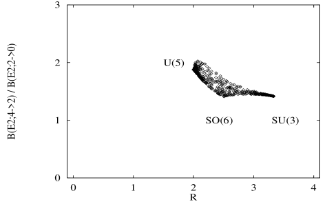
Energies by themselves are not sufficient to decide whether or not there exists a collective structure. Levels belonging to a collective band are connected by strong electromagnetic transitions. In Fig. 6 we show a correlation plot between the ratio of values for the and transitions and the energy ratio R. For the values we use the quadrupole operator
| (36) |
with . For completeness, in Table IV we show the results for the three symmetry limits of the IBM [6]. In the large limit, the ratio of values is 2 for the harmonic vibrator and 10/7 both for the -unstable rotor and the pure rotor. There is a strong correlation between the first peak in the energy ratio and the vibrator value for the ratio of values (the concentration of points in this region corresponds to about 50 of all cases), and for the second peak and the rotor value (about 25 of all cases) [21].
The results presented in Figs. 5 and 6 were obtained with random interactions, with no restriction on the sign nor the magnitude of the one- and two-body matrix elements. It is of interest to make a comparison with a calculation in which the parameters are restricted to the ‘physically’ allowed region. To this end, we consider the consistent-Q formulation [22] which uses the same form for the quadrupole operator, Eq. (36), i.e. with the same value of for the operator and the Hamiltonian
| (37) |
The parameters and are restricted to be positive, whereas can be either positive or negative . The properties of the Hamiltonian of Eq. (37) are investigated by taking the scaled parameters and randomly on the intervals and (these coefficients have been used as control parameters in a study of phase transitions in the IBM [8, 9]). In Figs. 7 and 8 we show the corresponding probability distribution and correlation plot for the consistent-Q formulation of the IBM with realistic interactions. Although in this case the points are concentrated in a smaller region of the plot than before, the results show the same qualititative behavior as with random one- and two-body interactions. In Fig. 8 we have identified each of the dynamical symmetries of the IBM (and the transitions between them). There is a large overlap between the regions with the highest concentration of points in Figs. 6 and 8.
These results, i.e. the dominance of ground states and the occurrence of both vibrational and rotational structures, are not based solely on energies, but also involve wave function information via the quadrupole transitions. The use of random interactions (both in magnitude and sign) show that these regular features arise from a much wider class of Hamiltonians than are generally considered to be realisitic, and are, to a certain extent, independent of the specific character of the interactions. This too is in qualitative agreement with the empirical observation of robust features in the low-lying spectra of medium and heavy even-even nuclei [1, 2]. This leads naturally to the question of what is the cause of this behavior, if the only ingredients of the calculations are the one- and two-body nature of the interactions, the number of bosons and the structure of the model space?
In order to see to what extent the results found above [21] depend on the rank of the interactions, we study the effect of the inclusion of three-body interactions in the Hamiltonian. Three-body interactions are of special interest in the IBM, since they can give rise to stable triaxial deformations [23], which are absent in the case of one- and two-body interactions only. We consider the most general one-, two- and three-body IBM Hamiltonian
| (38) |
where and are given in Eqs. (26) and (27). contains the 17 possible three-body random interactions and can be written in a similar fashion. Again we find a dominance (61.9 ) of ground states; in 12.0 of the cases the ground state has , and in 17.7 it has the maximum value of the angular momentum , very close to the results for the case of one- and two-body interactions only (63.4, 13.8 and 16.7 , respectively). Also the probability distribution shows the same behavior as for one- and two-body interactions. In Fig. 9 we compare the result for (solid curve, see Fig. 5) with . In both cases we see a very clear structure with pronounced peaks at the vibrational and rotational values of the energy ratio. Since the Hamiltonian depends on 26 independent random numbers (2 one-body, 7 two-body and 17 three-body matrix elements), there is less correlation between its many-body () matrix elements than in the case of . This results in somewhat less pronounced (lower and broader) – but nevertheless very clear – peaks in the probability distribution .
IV Summary and conclusions
In this work, we discussed global properties of nuclear structure using random Hamiltonians.
We first considered the problem from a shell model perspective, focussing on a system of identical neutrons in the shell. We confirmed the conclusion reached earlier by Johnson and collaborators [11, 12] that nuclei with many nucleons favor ground states, even without a dominant pairing component in the force. We demonstrated further that this is not a consequence of time-reversal invariance of the random Hamiltonian. Finally, we showed that systems of identical nucleons interacting via random two-body interactions tend to favor a seniority structure, in accord with conclusions reported recently in [13]. There is little or no evidence for the occurrence of vibrational and rotational bands.
We then considered the same issues in the context of the IBM, a collective model that from the outset emphasizes the role of monopole and quadrupole pairs. Here too we found that ground states predominate, exactly as in the shell model analysis. In contrast, we found that the IBM strongly favors both vibrational and rotational structures, as evident from energy ratios of low-lying states and their corresponding ratios. These conclusions emerged from a much wider class of Hamiltonians than is usually thought to be ‘realistic’. The inclusion of three-body random interactions did not change these basic conclusions, as long as the number of bosons is sufficiently large. This suggests that the observed vibrational and rotational features represent general and robust properties of the IBM model space, and do not depend significantly on details of the interaction. Since the structure of the model space is completely determined by the degrees of freedom, our results emphasize once again the importance of the selection of the relevant degrees of freedom.
The results that we obtained with random Hamiltonians in the shell model and the IBM are in qualitative agreement with the empirical observation of robust features in the low-lying spectra of medium and heavy even-even nuclei and their tripartite classification into seniority, anharmonic vibrator and rotor regimes [1, 2]. The analysis with random interactions shows that seniority arises as a global property of the shell model space, while vibrational and rotational bands arise as general features of the interacting boson model space. However, the IBM is based on the assumption that low-lying collective excitations in nuclei can be described as a system of interacting monopole and quadrupole bosons, which in turn are associated with generalized pairs of like-nucleons with angular momentum and . Therefore it would be very important to establish whether vibrational and rotational features can also arise from ensembles of random interactions in the nuclear shell model, if appropriate (minimal) restrictions are imposed on the parameter space.
Acknowledgements
It is a pleasure to thank Rick Casten, Jorge Flores and Franco Iachello for illuminating discussions. This work was supported in part by DGAPA-UNAM under project IN101997, by CONACyT under projects 32416-E and 32397-E, and by NSF under grant PHY-9970749.
REFERENCES
- [1] R.F. Casten, N.V. Zamfir and D.S. Brenner, Phys. Rev. Lett. 71, 227 (1993).
- [2] N.V. Zamfir, R.F. Casten and D.S. Brenner, Phys. Rev. Lett. 72, 3480 (1994).
- [3] R. Bijker, A. Frank and S. Pittel, Phys. Rev. C 55, R585 (1997).
- [4] N.V. Zamfir and R.F. Casten, Phys. Lett. B 341, 1 (1994).
- [5] R.V. Jolos, P. von Brentano, R.F. Casten and N.V. Zamfir, Phys. Rev. C 51, R2298 (1995).
- [6] F. Iachello and A. Arima, The interacting boson model (Cambridge University Press, 1987).
- [7] J.N. Ginocchio and M. Kirson, Phys. Rev. Lett. 44, 1744 (1980).
- [8] A.E.L. Dieperink, O. Scholten and F. Iachello, Phys. Rev. Lett. 44, 1747 (1980).
- [9] F. Iachello, N.V. Zamfir and R.F. Casten, Phys. Rev. Lett. 81, 1191 (1998).
- [10] R.F. Casten, D. Kusnezov and N.V. Zamfir, Phys. Rev. Lett. 82, 5000 (1999).
- [11] C.W. Johnson, G.F. Bertsch and D.J. Dean, Phys. Rev. Lett. 80, 2749 (1998).
- [12] C.W. Johnson, Rev. Mex. Fís 45 S2, 25 (1999).
- [13] C.W. Johnson, G.F. Bertsch, D.J. Dean and I. Talmi, Phys. Rev. C 61, 014311 (2000).
- [14] E.P. Wigner, Ann. of Math. 62, 548 (1955); Ann. of Math. 67, 325 (1958).
- [15] See e.g. the review T.A. Brody, J. Flores, J.B. French, P.A. Mello, A. Pandey and S.S.M. Wong, Rev. Mod. Phys. 53, 385 (1981).
- [16] J.B. French and S.S.M. Wong, Phys. Lett. B 33, 449 (1970); Phys. Lett. B 35, 5 (1971).
- [17] O. Bohigas and J. Flores, Phys. Lett. B 34, 261 (1971).
- [18] A. Gervois, Nucl. Phys. A 184, 507 (1972).
- [19] R. Bijker, A. Frank and S. Pittel, Phys. Rev. C 60, 021302 (1999).
- [20] J.B. French, V.K.B. Kota, A. Pandey and S. Tomsovic, Phys. Rev. Lett. 54, 2313 (1985).
- [21] R. Bijker and A. Frank, Phys. Rev. Lett. 84, 420 (2000).
- [22] D.D. Warner and R.F. Casten, Phys. Rev. Lett. 48, 1385 (1982).
- [23] P. van Isacker and J.Q. Chen, Phys. Rev. C 24, 684 (1981).
| Basis | GOE | ||||
|---|---|---|---|---|---|
| 2 | 0 | 3 | 2.00 | 21.4 | 15.9 |
| 1 | 2 | 1.73 | 14.3 | 4.9 | |
| 2 | 5 | 2.45 | 35.7 | 68.3 | |
| 3 | 2 | 1.73 | 14.3 | 6.1 | |
| 4 | 2 | 1.74 | 14.3 | 4.8 |
| Basis | TBRE | ||||
| 4 | 0 | 9 | 6.24 | 11.1 | 55.9 |
| 1 | 12 | 5.05 | 14.8 | 4.9 | |
| 2 | 21 | 5.37 | 25.9 | 22.7 | |
| 3 | 15 | 4.79 | 18.5 | 1.4 | |
| 4 | 15 | 5.12 | 18.5 | 12.3 | |
| 5 | 6 | 4.65 | 7.4 | 1.5 | |
| 6 | 3 | 4.69 | 3.7 | 1.3 | |
| 6 | 0 | 14 | 10.16 | 9.9 | 67.7 |
| 1 | 19 | 8.53 | 13.4 | 1.3 | |
| 2 | 33 | 9.01 | 23.2 | 15.0 | |
| 3 | 29 | 8.80 | 20.4 | 7.1 | |
| 4 | 26 | 8.80 | 18.3 | 6.8 | |
| 5 | 12 | 8.27 | 8.5 | 0.4 | |
| 6 | 8 | 8.61 | 5.6 | 1.7 | |
| 7 | 1 | 8.07 | 0.7 | 0.0 |
| TBRE | |
|---|---|
| 0.00 | 67.7 |
| 0.25 | 69.3 |
| 0.50 | 71.7 |
| 0.75 | 74.0 |
| 1.00 | 76.8 |