Dynamical constraints on phase transitions

Abstract

The numerical solutions of nonlocal and local Boltzmann kinetic equations for the simulation of central heavy ion reactions are parameterized in terms of time dependent thermodynamical variables in the Fermi liquid sense. This allows one to discuss dynamical trajectories in phase space. The nonequilibrium state is characterized by non-isobaric, non-isochoric etc. conditions, shortly called iso-nothing conditions. Therefore a combination of thermodynamical observables is constructed which allows one to locate instabilities and points of possible phase transition in a dynamical sense. We find two different mechanisms of instability, a short time surface - dominated instability and later a spinodal - dominated volume instability. The latter one occurs only if the incident energies do not exceed significantly the Fermi energy and might be attributed to spinodal decomposition. In contrast the fast surface explosion occurs far outside the spinodal region and pertains also in the cases where the system develops too fast to suffer a spinodal decomposition and where the system approaches equilibrium outside the spinodal region.

]

I Introduction

The collisions of heavy ions around the Fermi energy and the description of multifragmentation phenomena fills an enormous literature. Mostly the multifragmentation is attributed to a hypothetical liquid - gas phase transition which is partially supported by mean field considerations in equilibrium where the nonlinear density dependence of the interaction energy leads to a liquid - gas like first order phase transition. Therefore, the phenomena has been investigated in terms of a spinodal decomposition. However this straightforward picture is over-shadowed by at least two serious drawbacks. First we have to deal with finite systems, where the phase transition appears modified and less pronounced than in infinite bulk matter. And secondly, we have to face the fact that the process evolves under extreme nonequilibrium conditions. For a critical discussion of recent models on multifragmentation see [1]. We want to investigate the latter two points here and will use a microscopic approach which allows one to describe the time evolution of the one-particle distribution function including binary correlations. We will suggest a possibility of analyzing phase transitions in terms of time dependent thermodynamical variables and will be able, in this way, to see signals of instability in nonequilibrium and finite systems.

The standard treatment to investigate basic features of multifragmentation processes is performed in terms of fluctuation analysis starting from the Landau equation [2, 3, 4] or BUU equations [5, 6]. Observing that these kinetic equations do not lead to enough fluctuations to describe multifragmentation, additional stochasticity has been assumed and incorporated resulting in Boltzmann-Langevin pictures [7, 8, 9, 10, 11, 12]. The large time scale of fluctuations has been analyzed in [13]. It is found that the large time evolution of the system is guided by cooperative effects and fluctuations in a universal manner. The crucial role of collision rate has been pointed out in that it enforces the diffusive regime.

We will adopt here a straight microscopic picture of kinetic theory without additional fluctuations of Langevin sources. While this is perfectly microscopical controlled we have to leave out the possibility of describing fragment production. In contrast we will investigate the thermodynamical trajectories as arising straight from the solved kinetic equation as a Fermi liquid. Therefore no coalescence or other cluster creation mechanisms are used. This allows to restrict to the single particle distribution if the two - particle correlations are included in the collision integral. This is performed in the frame of the nonlocal kinetic theory. Since we want to study the dynamical constraints of phase transitions as necessary but not sufficient conditions we can expect already from the kinetic theory an answer whether the system will undergo spinodal decomposition or other forms of decomposition. In fact we will demonstrate that there is a dominant surface emission at higher energies than the Fermi energy while the spinodal decomposition can be accessed only for energies lower or equal the Fermi energy. For higher energies the system evolves too fast through the spinodal region to be influenced sufficiently by spinodal decomposition.

There are two experimental hints for two different regimes of instability in heavy ion collisions around Fermi energy. The first one concerns the emulsion data recorded in the experiment by F. Schussler et. al. which has been considered in [14]. There the fragments with charge $Z>2$ has been grouped into two different velocities, one around $0.16c$ and the other with $0.25c$. A possible interpretation has been advocated that the higher velocity group comes from fragments emitted at an early stage from the surface. The TDHF calculations seemed to support this picture.

A second experimental signal comes from the production of hard photons as measured by the TAPS collaboration [15]. The extracted source sizes by HBT interferometry has found to be too large if not two sources are assumed. Moreover the calculated photon spectra shows a clear prompt source of hard photons besides later thermal photons. The latter second source vanishes for incident energies larger than $60$MeV. This indicates already that there is a transition between two mechanisms of particle production and instability if the bombarding energy exceeds 50-60 MeV.

We will show that indeed there can be identified two mechanisms; at short times a surface dominated emission and at later times a volume dominated spinodal decomposition. For low energies we will find that the volume spinodal effects are visible while for higher energies only the surface emission survives.

II Kinetic description

We use for the description the recently derived nonlocal kinetic equation [16] for the one - particle distribution function

$${\partial f_{1}\over\partial t}+{\partial\varepsilon_{1}\over\partial{\bf k}}{\partial f_{1}\over\partial{\bf r}}-{\partial\varepsilon_{1}\over\partial{\bf r}}{\partial f_{1}\over\partial{\bf k}}=$$ (1)

$$\sum_{b}\int{d{\bf p}d{\bf q}\over(2\pi)^{5}\hbar^{7}}\delta\left(\varepsilon_{1}+\varepsilon_{2}-\varepsilon_{3}-\varepsilon_{4}+2\Delta_{E}\right)\left|{\cal T}_{ab}\right|^{2}=$$ (2)

$$\Bigl{[}f_{3}f_{4}\bigl{(}1-f_{1}\bigr{)}\bigl{(}1-f_{2}\bigr{)}-\bigl{(}1-f_{3}\bigr{)}\bigl{(}1-f_{4}\bigr{)}f_{1}f_{2}\Bigr{]},$$ (3)

with Enskog-type shifts of arguments [16]: $f_{1}\equiv f_{a}({\bf k,r},t)$, $f_{2}\equiv f_{b}({\bf p,r}\!-\!\Delta_{2},t)$, $f_{3}\equiv f_{a}({\bf k\!-\!q}\!-\!\Delta_{K},{\bf r}\!-\!\Delta_{3},t\!-\!\Delta_{t})$ , and $f_{4}\equiv f_{b}({\bf p\!+\!q}\!-\!\Delta_{K},{\bf r}\!-\!\Delta_{4},t\!-\!\Delta_{t})$ . The effective scattering measure, the ${\cal T}$-matrix is centered in all shifts. The quasiparticle energy $\varepsilon$ contains the mean field as well as the correlated self energy.

In agreement with [17, 18], all gradient corrections are given by derivatives of the scattering phase shift $\phi={\rm Im\ ln}{\cal T}^{R}_{ab}(\Omega,{\bf k,p,q,}t,{\bf r})$,

$$\begin{array}[]{lclrcl}\Delta_{t}&=&{\displaystyle\left.{\partial\phi\over\partial\Omega}\right|_{\varepsilon_{1}+\varepsilon_{2}}}&\ \ \Delta_{2}&=&{\displaystyle\left({\partial\phi\over\partial{\bf p}}-{\partial\phi\over\partial{\bf q}}-{\partial\phi\over\partial{\bf k}}\right)_{\varepsilon_{1}+\varepsilon_{2}}}\\ &&&&&\\ \Delta_{E}&=&{\displaystyle\left.-{1\over 2}{\partial\phi\over\partial t}\right|_{\varepsilon_{1}+\varepsilon_{2}}}&\Delta_{3}&=&{\displaystyle\left.-{\partial\phi\over\partial{\bf k}}\right|_{\varepsilon_{1}+\varepsilon_{2}}}\\ &&&&&\\ \Delta_{K}&=&{\displaystyle\left.{1\over 2}{\partial\phi\over\partial{\bf r}}\right|_{\varepsilon_{1}+\varepsilon_{2}}}&\Delta_{4}&=&{\displaystyle-\left({\partial\phi\over\partial{\bf k}}+{\partial\phi\over\partial{\bf q}}\right)_{\varepsilon_{1}+\varepsilon_{2}}}.\end{array}$$ (4)

After derivatives, $\Delta$’s are evaluated at the energy shell $\Omega\to\varepsilon_{3}+\varepsilon_{4}$. Neglecting these shifts the usual BUU scenario appears.

The $\Delta$’s in the arguments of the distribution functions in (3) remind the non-instant and non-local corrections in the scattering-in integral for classical particles. The displacements of the asymptotic states are given by $\Delta_{2,3,4}$. The time delay enters in an equal way the asymptotic states 3 and 4. The momentum gain $\Delta_{K}$ also appears only in states 3 and 4. Finally, there is the energy gain which is discussed in [19]. These nonlocal corrections to the usual Boltzmann equation are a compact form of gradient corrections. It ensures that the conservation laws contain besides the mean-field correlations also the two particle correlations.

Despite its complicated form it is possible to solve this kinetic equation with standard Boltzmann numerical codes and to implement the shifts [20]. Therefore we have calculated the shifts for different realistic nuclear potentials [21]. The numerical solution of the nonlocal kinetic equation has shown an observable effect in the dynamical particle spectra of around $10\%$. The high energetic tails of the spectrum are enhanced due to more energetic two-particle collisions in the early phase of nuclear collision. Therefore the nonlocal corrections lead to an enhanced production of preequilibrium high energetic particles.

Besides the nonlocal shifts and cross section which has been calculated from realistic potentials we adopt here the view that the selfenergy $\varepsilon$ is parameterized in terms of the Skyrme potential for which we use a soft potential of the form

$$\varepsilon={p^{2}\over 2m}+A\left({n\over n_{0}}\right)+B\left({n\over n_{0}}\right)^{\sigma}.$$ (5)

For a derivation of collision integrals and the Skyrme potential (5) from the same microscopic footing, see [22].

A Balance equations

By multiplying the kinetic equation with $1,{\bf p},\varepsilon$ one obtains the balance for the particle density $n$, the momentum density $J$ and the energy density ${\cal E}$. Without nonlocal corrections the collision integrals vanish for the density and momentum balance and we get the standard balance equations for the quasiparticle parts

$${\partial n_{a}({\bf r},t)\over\partial t}+{\bf{\partial\over\partial r}}\int{d{\bf p}\over(2\pi\hbar)^{3}}{\partial\varepsilon\over\partial{\bf p}}f_{a}({\bf p,r},t)=0$$ (6)

$${\partial J_{i}({\bf r},t)\over\partial t}+{\partial\over\partial r_{j}}{\cal P}^{\rm qp}_{ij}=0$$ (7)

with the quasiparticle density, the current and the momentum tensor

$$n_{a} = \int{d{\bf p}\over(2\pi\hbar)^{3}}f_{a}$$ (8)

$${\bf J}({\bf r},t) = \int{d{\bf p}\over(2\pi\hbar)^{3}}\,{\bf p}\,f_{a}({\bf p,r},t)$$ (9)

$${\cal P}_{ij}^{\rm qp} = \sum_{a}\int{d{\bf p}\over(2\pi\hbar)^{3}}\left(p_{j}{\partial\varepsilon_{a}\over\partial p_{i}}+\delta_{ij}\varepsilon_{a}\right)f_{a}-\delta_{ij}{\cal E}^{\rm qp}$$ (10)

where the quasiparticle energy is given by

$${\cal E}^{\rm qp} = \sum_{a}\int{d{\bf p}\over(2\pi\hbar)^{3}}{p^{2}\over 2m}f_{a}$$ (11)

$$+ {1\over 2}\sum_{a,b}\int{d{\bf k}d{\bf p}\over(2\pi\hbar)^{6}}{\cal T}_{ab}(\varepsilon_{1}+\varepsilon_{2},{\bf k,p},0)f_{a}f_{b}$$ (12)

and the pressure is as usual

$$P=\frac{1}{3}{\cal P}_{ii}.$$ (13)

The quasi particle energy of the system varies as

$$\delta{\cal E^{\rm qp}} = \int{d{\bf p}\over(2\pi\hbar)^{3}}{\delta{\cal E}^{\rm qp}\over\delta f({\bf p,r},t)}\delta f({\bf p,r},t)$$ (14)

$$= \int{dp\over(2\pi\hbar)^{3}}\varepsilon\delta f({\bf p,r},t)$$ (15)

and since we adopt the parameterization of quasiparticle energy (5), the quasiparticle part of the total energy density reads

$${\cal E}^{\rm qp}({\bf r},t)=\sum\limits_{a}\int{d{\bf p}\over(2\pi\hbar)^{3}}{p^{2}\over 2m}f_{a}({\bf p,r},t)$$ (16)

$$+{A}{\textstyle\frac{n^{2}({\bf r},t)}{2n_{0}}}+B{\textstyle\frac{n({\bf r},t)^{\sigma+1}}{(\sigma+1)n_{0}^{\sigma}}}+{\cal E}^{\rm Born}.$$ (17)

Please note that besides the mean field (5) we have also a Born correlation term ${\cal E}^{\rm Born}$ coming from the second term of (12), see [23],

$${\cal E}^{\rm Born}(t) = {{\cal E}_{F}^{2}}{2\log 2-11\over 70\pi^{3}}{m\over\hbar^{2}}{\sigma}+o(T^{3}).$$ (18)

The balance of the quasiparticle part of the energy density reads from the kinetic equation

$${\partial{\cal E}^{\rm qp}({\bf r},t)\over\partial t}+{\bf{\partial\over\partial r}}\sum\limits_{a}\int{d{\bf p}\over(2\pi\hbar)^{3}}\varepsilon_{a}{\partial\varepsilon_{a}\over\partial{\bf p}}f_{a}({\bf p,r},t)=0.$$ (19)

The correlational parts of the density, pressure and energy are coming from genuine two-particle correlations beyond Born approximation which are also derived from the balance equations of nonlocal kinetic equations [16]. It has been shown that they establish the complete conservation laws. These $\Delta$-contributions following from the nonlocality of the scattering integral read for the energy, pressure tensor and density

$${\cal E}_{c} = {1\over 2}\sum_{a,b}\int{d{\bf k}d{\bf p}d{\bf q}\over(2\pi\hbar)^{9}\hbar}\,\Psi\,[\varepsilon_{1}+\varepsilon_{2}]\Delta_{t},$$ (20)

$${\cal P}^{c}_{ij} = \!{1\over 2}\!\sum_{a,b}\!\!\int\!{d{\bf k}d{\bf p}d{\bf q}\over(2\pi\hbar)^{9}\hbar}\Psi\left[(p\!+\!q)_{i}\Delta_{4j}\!+\!(k\!-\!q)_{i}\Delta_{3j}\!-\!p_{i}\Delta_{2j}\right],$$ (21)

$$n_{c} = \sum_{b}\int{d{\bf k}d{\bf p}d{\bf q}\over(2\pi\hbar)^{9}\hbar}\Psi\Delta_{t},$$ (22)

where $\Psi=|{\cal T}_{\rm ab}^{R}|^{2}2\pi\delta(\varepsilon_{1}\!+\!\varepsilon_{2}\!-\!\varepsilon_{3}\!-\!\varepsilon_{4})f_{1}f_{2}(1\!-\!f_{3}\!-\!f_{4})$ is the probability to form a molecule during the delay time $\Delta_{t}$.

While these correlated parts are present in the numerical results and can be shown to contribute to the conservation laws we will only discuss the thermodynamical properties in terms of quasiparticle quantities to compare as close as possible with the mean field or local BUU expressions. The discussion of these correlated two - particle quantities are devoted to a separate consideration.

B Dynamical thermodynamical variables

We want now to construct the time dependent global termodynamical variables. From the distribution function $f({\bf p,r},t)$ the local density, current and energy densities are given by

$${n}({\bf r},t) = \displaystyle{\int{d{\bf p}\over(2\pi\hbar)^{3}}{f({\bf p,r},t)}}$$ (23)

$${\bf J}({\bf r},t) = \displaystyle{\int{d{\bf p}\over(2\pi\hbar)^{3}}{\bf p}{f({\bf p,r},t)}}$$ (24)

$${\cal E}_{K}({\bf r},t) = \displaystyle{\int{d{\bf p}\over(2\pi\hbar)^{3}}{p^{2}\over 2m}{f({\bf p,r},t)}}$$ (25)

which are computed directly from the numerical solution of the kinetic equation in terms of test particles. Please note that the above kinetic energy includes the Fermi motion.

1 Temperature

The global variables per particle number like kinetic energy, Fermi energy and collective energy are obtained by spatial integration

$${\cal E}_{K}(t) = {\displaystyle{\int d{\bf r}\,{\cal E}_{K}({\bf r},t)}\over\displaystyle{\int d{\bf r}\,{n}({\bf r},t)}}$$ (26)

$${\cal E}_{F}(t) = {\displaystyle{\int d{\bf r}\,{\cal E}_{f}[{n}({\bf r},t)]{n}({\bf r},t)}\over\displaystyle{\int d{\bf r}\,{n}({\bf r},t)}}$$ (27)

$${\cal E}_{\rm coll}(t) = {\displaystyle{\int d{\bf r}\,{{J}({\bf r},t)^{2}\over m\,{n}({\bf r},t)}}\over\displaystyle{\int d{\bf r}\,{n}({\bf r},t)}}$$ (28)

where we have used the local density approximation [24]. Now we adopt the picture of Fermi liquid theory which connects the temperature with the kinetic energy as

$${\cal E}_{K}(t)=\frac{3}{5}{\cal E}_{F}(t)+{\cal E}_{\rm coll}(t)+{\pi^{2}\over 4{\cal E}_{F}(t)}{T(t)}^{2}$$ (29)

from which we deduce the global temperature. The definition of temperature is by no means obvious since it is in principle an equilibrium quantity. One has several possibilities to define a time dependent equivalent temperature which should approach the equilibrium value when the system approaches equilibrium. In [25, 26] the definition of slope temperatures has been discussed and compared to local space dependent temperature fits of the distribution function of matter. This seems to be a good measure for higher energetic collisions in the relativistic regime. Since we restrict here to collisions in the Fermi energy domain and do not want to add coalescence models we will not use the slope temperature. Moreover we define the global temperature in terms of global energies which are obtained by local quantities rather than defining a local temperature itself. This has the advantage that we do not consider local energy fluctuations but only a mean evolution of temperature.

2 Energy and pressure

The mean field part of the energy is given by

$$U(t) = {\cal E}^{\rm qp}(t)-{\cal E}_{K}(t)-{\cal E}^{\rm Born}(t)$$ (30)

$$= {\displaystyle{\int d{\bf r}\left(A{{n({\bf r},t)}^{2}\over 2n_{0}}+B{{n({\bf r},t)}^{s+1}\over(s+1)n_{0}^{s}}\right)}\over\displaystyle{\int d{\bf r}\,{n}({\bf r},t)}}$$ (31)

from which one deduces the pressure per particle

$$P(t) = \frac{2}{3}({\cal E}_{K}(t)-{\cal E}_{\rm coll}(t))+\frac{4}{3}{\cal E}^{\rm Born}(t)$$ (32)

$$+ {\displaystyle{\int d{\bf r}\left(A{{n({\bf r},t)}\over 2n_{0}}+B{s\,{n({\bf r},t)}^{s}\over(s+1)n_{0}^{s}}\right)}\over\displaystyle{\int d{\bf r}\,{n}({\bf r},t)}}.$$ (33)

In order to compare now the local BUU with the nonlocal BUU scenario we consider the energy which would be the total energy in the local BUU without Coulomb energy

$${\cal E}(t)={\cal E}_{K}(t)-{\cal E}_{\rm coll}(t)+U(t).$$ (34)

This expression does not contain the two - particle correlation energy which is zero for BUU and the Coulomb energy. The reason for considering this energy for dynamical trajectories is that we want to follow the trajectories in the picture of mean field and usual spinodal plots.

3 Density

To define the density exhibits to some extend a problem. To illustrate this fact we have plotted in figure 1 and 2 the density evolution. We see that depending on the considered volume sphere we obtain different global densities. We follow here the point of view that the mean square radius will be used as a sphere to define the global density. This is also supported by the observation that the mean square radius follows the visible compression. This becomes evident in figure 2 for a symmetric reaction at higher energies where at $40$fm/c we see a clear compression. If we define the volume by a density cut $n>n_{0}/10$ in spatial domain we will not see compression at all since the matter is evaporating and this volume increases correspondingly to compression. Therefore we think that the sphere with the mean square radius is a good compromise.

III Iso-nothing conditions in equilibrium

Let us first recall the figures of mean field isotherms in equilibrium. The mean field Skyrme and Born correlational energy is

$${\cal E}=\frac{3}{2}nT{f_{5/2}\over f_{3/2}}+{A\over 2n_{0}}n^{2}+{B\over(s+1)n_{0}}n^{s+1}+{\cal E}^{\rm Born}$$ (35)

with the kinetic energy in terms of standard Fermi integrals and the density

$$n={g\over\lambda^{3}}f_{3/2}$$ (36)

with $g$ the spin, isospin,… degeneracy. The corresponding pressure reads

$$P = n^{2}{d({\cal E}/n)\over dn}$$ (37)

$$= nT{f_{5/2}\over f_{3/2}}+{A\over 2n_{0}}n^{2}+{Bs\over(s+1)n_{0}}n^{s+1}.$$ (38)

We obtain the typical van der Waals curves in figure 3. Since we have neither isothermal nor isochoric nor isobaric conditions in simulations, shortly since we have iso-nothing conditions, we have to find a representation of the phase transition curves which are independent of temperature but which reflects the main features of phase transitions. This can be achieved by the product of energy and pressure density versus energy density in figure 3 below. This plot shows that all instable isotherms exhibit a minimum in the left lower quarter. There the energy is negative denoting bound state conditions but the pressure is already positive which means the system is unstable. The first isotherm above the critical one does not touch this quarter but remains in the right upper quarter where the energy and pressure are both positive and the system is expanding and decomposing unboundly. The left upper quarter denotes negative pressure and energy indicating that the system is bound and stable.

FIG. 1.: The time evolution of central collisions $Ni+Au$ at $25$MeV per nucleon. The density contours in the spatial plane $(x,0,Z)$ is plotted in the left figure in the range $-15,15$fm and the arrows characterize the values of the local current $J$ according to (25). The middle figure gives the density profile in ${\rm fm}^{-3}$ of the beam direction (solid line) and perpendicular to the beam (dotted line). The corresponding right panel shows the global density ratio to nuclear density $no=0.16{\rm fm}^{-3}$ defined in a sphere versus the radius of the sphere. The mean square radius is marked explicitly by a dot on the radius axes.

FIG. 2.: The time evolution of central collisions $Xe+Sn$ at $50$MeV per nucleon analogous to figure 1.

FIG. 3.: The isotherms for the pressure density versus volume (above) and for the product of pressure and energy density versus energy density (below). The temperatures are $T=1,4,7,10,13,16,19$MeV.

In order to achieve now a temperature independent plot we scale both axes of figure 3 (below) with a temperature dependent polynomial and achieve that all critical isotherms are collapsing on one curve in the left lower quarter, see figure 4.

FIG. 4.: The isotherms of the product of pressure and energy density versus energy density scaled by a temperature polynomial $f(T)$, $g(T)$. The temperatures are $T=1,4,7,10,13,16,19$MeV respectively. All critical isotherms collapse on one line in the left lower quarter.

The first isotherms above the critical one does not enter the left lower quarter. We consider this scaling as adequate for iso-nothing conditions. A phase transition should be possible to observe if there occurs a minimum in the left half of this plot at negative energies.

The idea of plotting combinations of pressure and energy is similar to the one of softest point [27] in analyzing QCD phase transitions. There the simple pressure over energy ratio leads to a temperature independent plot due to ultrarelativistic energy - temperature relations. In our case we have a Fermi liquid behavior at low temperatures and have to scale differently. In particular we have used in figure 4 the temperature dependent polynomials

$$g[x=T/{\rm MeV}] = 1.2+\frac{1}{3}10^{-1}x+\frac{1}{3}10^{-3}x^{2}+\frac{1}{5}10^{-4}x^{4}$$ (40)

$$+\frac{1}{8}10^{-6}x^{6}$$

$$f[x=T/{\rm MeV}] = 1.2+\frac{1}{3}10^{-2}x+\frac{1}{3}10^{-2}x^{2}+10^{-5}x^{4}$$ (42)

$$+10^{-7}x^{6}$$

which are producing a temperature independent plot in figure 4 for the specific used mean field potential parameterization.

IV Nonequilibrium thermodynamics

Let us now inspect the dynamical trajectories for the above defined temperature, density and energy. In figure 5 we have plotted the dynamical trajectories for a charge - symmetric reaction of $Xe$ on $Sn$ at $25$MeV lab - energy. The solution of the nonlocal kinetic equation is compared to the local BUU one. One sees in the temperature versus density plane that the point of highest compression is reached around $60$fm/c with a temperature of $9$ MeV.

After this point of highest overlap or fusion phase we have an expansion phase where the density and temperature is decreasing. While the compression phase is developing similar for the BUU and for the nonlocal kinetic equation we see now differences in the development. First the temperature of the nonlocal kinetic equation is around $2$MeV higher than the local BUU result. This is due to the release of correlation energy into kinetic energy which is not present in the local BUU scenario. After this expansion stage until times of $120$fm/c we see that the BUU trajectories come to a rest inside the spinodal region while the nonlocal scenario leads to a further decay. This can be seen by the continuous decrease of density and increase of energy. Since matter is more decomposed with the nonlocal kinetic equation we also heat the system more due to Coulomb acceleration. This leads to the enhancement of temperature compared to BUU. An oscillating behavior occurs at later times which reflects an interplay between short range correlation and long range Coulomb repulsion. The decomposition leads almost to free gaseous matter after $300$fm/c as can be seen in the energy versus density plot.

Please note that although the trajectories seems to equilibrate inside the spinodal region when one considers the temperature versus density plane, we see that in the corresponding energy versus temperature plane the trajectories travel already outside the spinodal region. This underlines the importance to investigate the region of spinodal decomposition in terms of a three dimensional plot instead of a two dimensional one like in the recently discussed caloric curve plots. Different experimental situations lead to different curves as long as the third coordinate (pressure or density) remains undetermined.

The iso-nothing plot analog to figure 4 in the lower left corner shows that the point of highest compression is linked to a first instability seen as a pronounced minimum of the trajectory in the left quarter. This is connected with a pronounced surface emission and connected with anomalous velocity profiles [28]. We will call this phase surface emission instability further on. At $180$ fm/c we see a second minimum which is taking place inside the spinodal region. This instability we might now attribute to spinodal decomposition since the trajectories developing slower and remain inside the spinodal region. The BUU shows the same qualitative minima but the matter rebounds and the trajectories move towards negative energies again. In opposition the nonlocal scenario leads to a further decomposition of matter as described above.

In the next figure 6 we have plotted the same reaction as in figure 5 but at higher energy of $33$MeV. We recognize a higher compression density and temperature than compared to the lower bombarding energy. Consequently the trajectories develop further towards the unbound region of positive energy after $300$fm/c. While the first surface emission instability is strongly pronounced we see that the second minimum in the iso-nothing plot is already weaker indicating that the role of spinodal decomposition is diminished. The trajectories in the temperature versus density plot comes still in the spinodal region at rest but travels already outside the spinodal region if the energy versus temperature plot is considered. This shows that the trajectories start to develop too fast to suffer much spinodal decomposition.

If we now plot the same reaction at $50$MeV in figure 7 we see that the trajectories come at rest outside the spinodal region whatever plot is used and no second minima is seen anymore in the iso-nothing plot. But, the surface emission instability is still very pronounced and is probably here the leading mechanism of matter disintegration.

We might now search for a situation where we have the opposite extreme that is we search for a reaction with as less as possible surface emission instability and as much as possible spinodal decomposition. For this reason we might think on asymmetric reactions since the different sizes of the colliding nuclei might suppress the surface emission. Indeed as can be seen in figure 8 for an asymmetric reaction of $Ni$ on $Au$ at $25$MeV lab-energy with nearly the same total charge as in the reaction before that the surface emission instability is less pronounced while the spinodal instability is much more important. There appears even a third minima showing that the matter suffers spinodal decomposition perhaps more than once if the bombarding energy is low enough and a long oscillating piece of matter is developing.

The higher bombarding energies now show the same qualitative effect in that it pronounces the surface emission instability and reduces the importance of the spinodal decomposition as can be seen in figures 9 and 10. Please note that much smaller compression densities and temperatures are reached in these reactions compared to the more symmetric case of $Xe$ on $Sn$.

V Summary

The nonlocal kinetic theory leads to a different nonequilibrium thermodynamics compared to the local BUU. We see basically a higher energetic particle spectra and a higher temperature of $2$MeV. This is attributed to the conversion of two-particle correlation energy into kinetic energy which is of course absent in local BUU scenario.

By constructing a temperature independent combination of thermodynamical variables we are able to investigate the signals of phase transitions under iso-nothing conditions. Two mechanisms of instability have been identified: surface emission instability and spinodal decomposition. We predict for the currently investigated reactions seen in table I which effect should be the leading one for matter decomposition.

25 MeV 33 MeV 50 MeV ${}^{58}_{28}$Ni + ${}^{197}_{79}$Au S C S C ( S) ${}^{129}_{54}$Xe + ${}^{119}_{50}$Sn C S C ( S) C

15 MeV 33 MeV 60 MeV ${}^{157}_{64}$Gd + ${}^{238}_{92}$U – C S C ${}^{181}_{73}$Ta + ${}^{197}_{79}$Au C S C ( S) C

TABLE I.: The prediction of the leading mechanisms of matter disintegration for two reactions with equal total charge but asymmetric entrance channels. Surface compression is denoted by $C$ and spinodal decomposition by $S$. In the reactions with bombarding energies higher than the Fermi energy the fast surface eruption happens outside the spinodal region. For even higher energies there is not enough time for the system to rest at the spinodal region. The trajectories simply move through the spinodal and the system decays before it comes to an equilibrium - like state inside the spinodal region.

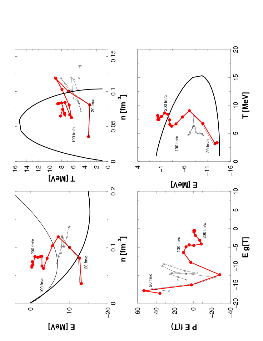
FIG. 5.: The dynamical trajectories of the energy (34), density and temperature (29) in the nonlocal (gray thick) and in the local BUU (black thin) scenario. The considered reaction is ${}^{129}Xe$ on ${}^{119}Sn$ at $25$MeV lab energy. The dots mark the times in steps of $20$fm/c up to total of $300$fm/c. To guide the eye the zero temperature mean field energy (thick line) and the pressure (thin line) is plotted in the upper left picture and in the right figures the spinodal line for infinite matter is given. The scaled combinational plot analogous to figure 4 is given in the left lower plane.

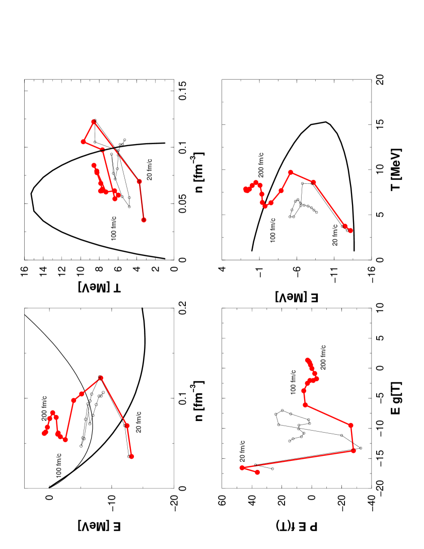
FIG. 6.: The same figure as 5 but for $33$MeV lab energy.

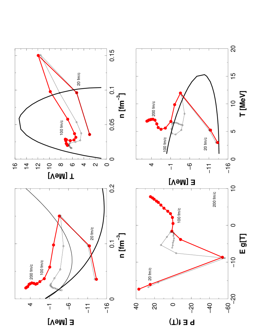
FIG. 7.: The same figure as 5 but for $50$MeV lab energy.

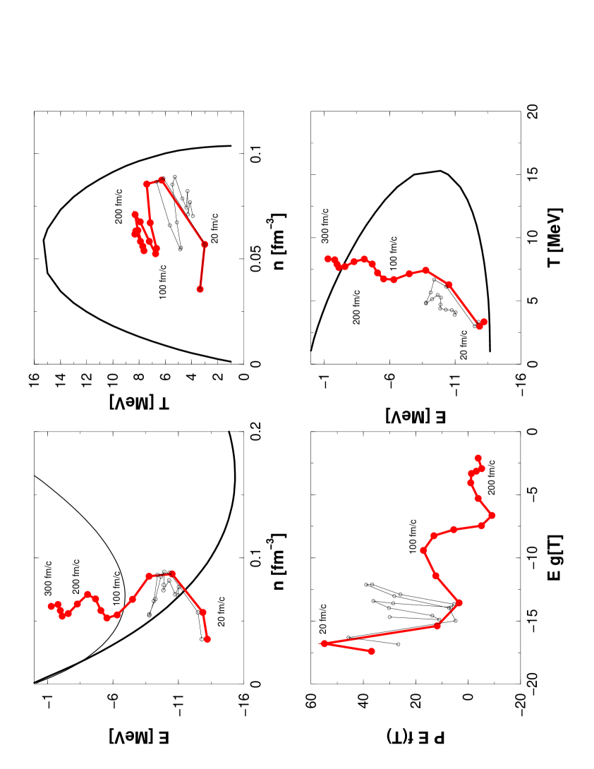
FIG. 8.: The same dynamical trajectories as in figure (5) but for a reaction ${}^{56}Ni$ on ${}^{179}Au$ at $25$MeV lab energy.

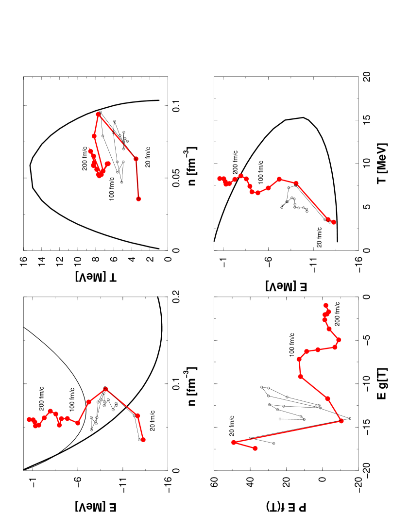
FIG. 9.: The same figure as 8 but for $33$MeV lab energy.

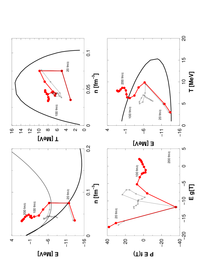
FIG. 10.: The same figure as 8 but for $50$MeV lab energy. Please note that the time point of highest compression is between $20$fm/c and $40$fm/c and not resolved.

- [1] J. B. Elliott and A. S. Hirsch, (2000), nucl-th/9912037.
- [2] C. Pethik and D. Ravenhall, Nucl. Phys. A 471, 19c (1987).
- [3] R. Donangelo, C. O. Dorso, and H. D. Marta, Phys. Lett. B 263, 19 (1991).
- [4] R. Donangelo, A. Romanelli, and A. C. S. Schifino, Phys. Lett. B 263, 342 (1991).
- [5] D. Kiderlen and H. Hofmann, Phys. Lett. B 332, 8 (1994).
- [6] S. Ayik, M. Colonna, and P. Chomaz, Phys. Lett. B 353, 417 (1995).
- [7] E. Suraud, S. Ayik, J. Stryjewski, and M. Belkacem, Nucl. Phys. A 519, 171c (1990).
- [8] S. Ayik and C. Gregoire, Nucl. Phys. A 513, 187 (1990).
- [9] J. Randrup and B. Remaud, Nucl. Phys. A 514, 339 (1990).
- [10] S. Ayik, E. Suraud, M. Belkacem, and D. Boilley, Nucl. Phys. A 545, 35 (1992).
- [11] M. Colonna et al., Phys. Rev. C 47, 1395 (1993).
- [12] M.Colonna, Ph.Chomaz, and J.Randrup, Nucl.Phys. A 567, 637 (1994).
- [13] S. Chattopadhyay, Phys. Rev. C 53, 1065 (1996).
- [14] H. Ngo et al., in Proceedings of the international workshop (GSI, Hirschegg, Kleinwalsertal, 1993), p. 302.
- [15] Y. Schutz and et. al., Nucl. Phys. A 622, 404 (1997).
- [16] V. Špička, P. Lipavský, and K. Morawetz, Phys. Lett. A 240, 160 (1998).
- [17] P. J. Nacher, G. Tastevin, and F. Laloe, Ann. Phys. (Leipzig) 48, 149 (1991).
- [18] M. de Haan, Physica A 164, 373 (1990).
- [19] P. Lipavský, V. Špička, and K. Morawetz, Phys. Rev. E 59, R 1291 (1999).
- [20] K. Morawetz et al., Phys. Rev. Lett. 82, 3767 (1999).
- [21] K. Morawetz, P. Lipavský, V. Špička, and N. Kwong, Phys. Rev. C 59, 3052 (1999).
- [22] K. Morawetz, sub: nucl-th/0003068 (2000).
- [23] K. Morawetz and H. Köhler, Eur. Phys. J. A 4, 291 (1999).
- [24] P. Schuck et al., Prog. Part. Nucl. Phys. 22, 181 (1989).
- [25] T. Gaitanos, H. Wolter, and C. Fuchs, (2000), sub: nucl-th/0003043.
- [26] T. Gaitanos, H. Wolter, and C. Fuchs, Phys. Lett. B 478, 79 (2000).
- [27] C. M. Hung and E. V. Shuryak, Phys. Rev. Lett. 75, 4003 (1995).
- [28] K. Morawetz, S. Toneev, and M. Ploszajczak, Phys. Rev. C (2000), sub.