Gradient terms in the microscopic description of K-atoms

We analyze the spectra of kaonic atoms using optical potentials with non-local (gradient) terms. The magnitude of the non-local terms follows from a self consistent many-body calculation of the kaon self energy in nuclear matter, which is based on s-wave kaon nucleon interactions. The optical potentials exhibit strong non-linearities in the nucleon density and sizeable non-local terms. We find that the non-local terms are quantitatively important in the analysis of the spectra and that a phenomenologically successful description can be obtained for p-wave like optical potentials. It is suggested that the microscopic form of the non-local interaction terms is obtained systematically by means of a semi-classical expansion of the nucleus structure. The resulting optical potential leads to less pronounced non-local effects.

and

^a Gesellschaft für Schwerionenforschung GSI, Postfach 110552, D-64220 Darmstadt, Germany 

^b H. Niewodniczański Institute of Nuclear Physics ul. Radzikowskiego 152, PL-31-342 Kraków, Poland 

PACS numbers: 36.10.-k, 13.75.Jz

1 Introduction

Kaonic atom data provide a valuable consistency check on any microscopic theory of the $K^{-}$ nucleon interaction in nuclear matter. We therefore apply the microscopic approach, developed by one of the authors in [1], to kaonic atoms. The description of the nuclear level shifts in $K^{-}$ atoms has a long history. For a recent review see [2]. We recall here the most striking puzzle. In the extreme low-density limit the nuclear part of the optical potential, $U_{\rm opt.}$, is determined by the s-wave $K^{-}N$ scattering length:

$$2\,\mu\,\,U_{\rm opt.}\left(\vec{r}\,\right)=-4\,\pi\left(1+\frac{m_{K}}{m_{N}}\right)a_{KN}\,\rho(r)$$ (1)

with $a_{KN}={\textstyle{1\over 4}}\,a_{KN}^{(I=0)}+{\textstyle{3\over 4}}\,\,a_{KN}^{(I=1)}\simeq\left(-0.18+0.67\,i\right)\,\mbox{fm}$, the nucleus density profile $\rho(r)$ and the reduced kaon mass $\mu$ of the $K^{-}$ nucleus system. As shown by Friedman, Gal and Batty [3] kaonic atom data can be described with a large attractive effective scattering length $a_{\rm eff.}\simeq\left(0.63+0.89\,i\right)$ fm, which is in direct contradiction to the low-density optical potential (1). The present data set on kaonic level shifts include typically the 3d$\to$2p transition for light nuclei and the 4f$\to$3d transition for heavy nuclei. Deeply bound kaonic states in an s-wave have not been observed so far. Since a $K^{-}$ bound in a p-wave at a nucleus probes dominantly the low-density tail of the nucleus profile one may conclude that the optical potential must exhibit a strong non-linear density characteristic at rather low density.

A further complication was pointed out for example by Thies [4], who demonstrated that in the kaonic ${}^{12}_{6}C$ system non-local effects may be important. The importance of non-local effects was also emphasized in [5, 6]. In fact a reasonable description of kaonic atom level shifts was achieved by Mizoguchi, Hirenzaki and Toki [7] with a phenomenological non-local optical potential of the form

$$2\,\mu\,\,U_{\rm opt.}\left(\vec{r},\vec{\nabla}\right)=-4\,\pi\left(1+\frac{m_{K}}{m_{N}}\right)\left(a_{KN}\,\rho(r)-b\,\vec{\nabla}\,\rho(r)\cdot\vec{\nabla}\right)\;,$$ (2)

where the parameter $b\simeq(0.47+i\,0.30)$ fm³.

Though it has been long anticipated that the $\mathchar 3\relax(1405)$ resonance plays a key role [5, 6, 7, 8], a microscopic description of kaonic atom data remains a challenge. Obviously an important ingredient of any such attempt must be a proper many-body treatment of the $\mathchar 3\relax(1405)$ resonance structure in nuclear matter.

2 Kaon self energy in nuclear matter

In this section we prepare the ground for our study of kaonic atoms. Of central importance is the kaon self energy, $\mathchar 5\relax_{K}(\omega,\vec{q}\,;\rho)$, evaluated in nuclear matter. Here we introduce the self energy relative to all vacuum polarization effects, i.e. $\mathchar 5\relax_{K}(\omega,{\vec{q}}\,;0)=0$.

First we recall results for the kaon self energy as obtained in a self consistent many-body calculation based on microscopic s-wave kaon-nucleon interactions. For the details of this microscopic approach we refer to [1]. We identify the $K^{-}$-nucleus optical potential $V_{\rm opt.}(\vec{q}\,)$ by

$$2\,E_{K}({\vec{q}}\,)\,V_{\rm opt.}({\vec{q}}\,)=\mathchar 5\relax_{K}(\omega=E_{K}({\vec{q}}\,),{\vec{q}}\,)\;,$$ (3)

where $E_{K}({\vec{q}}\,)=(m_{K}^{2}+{\vec{q}}\,^{2})^{1/2}$ is the free-space kaon energy. In Fig. 1 we present the result of [1]

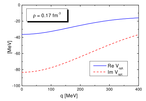
Fig. 1: The $K^{-}$ nuclear optical potential, $V_{\rm opt.}(\vec{q}\,)$, plotted as a function of the kaon three momentum. The nuclear density is $\rho=0.17$ fm^-3.

at nuclear saturation density. We point out that the real part of our optical potential exhibits rather moderate attraction of less than 40 MeV. On the other hand we find a rather strong absorptive part of the optical potential. This is in disagreement with recent work by Friedman, Gal, Mares and Cieply [9]. We recall that in [1] the quasi-particle energy for a $K^{-}$ at rest was found to be $380$ MeV at nuclear saturation density and that the large attraction in the quasi-particle energy is consistent with the moderate attraction in the optical potential. It merely reflects the strong energy dependence of the kaon self energy induced by the $\mathchar 3\relax(1405)$ resonance. Such important energy variations are typically missed in a mean field approach. Hence, a proper treatment of the pertinent many-body effects is mandatory.

We analyze the self energy as probed in kaonic atoms in more detail. Before we proceed it is important to straighten out the relevant scales. Since the typical binding energy of a $K^{-}$ bound at a nucleus in a p-wave is of the order of 0.5 MeV the typical kaon momentum is estimated to be roughly 20 MeV. We then expect the relevant nuclear Fermi momentum $k_{F}$ to be larger than the kaon momentum $|\vec{q}\,|<k_{F}$.

Fig. 2: The effective scattering length $a_{\rm eff.}(k_{F})$ and effective slope parameters $b_{\rm eff.}(k_{F})$ and $c_{\rm eff.}(k_{F})$ as defined in (4). The solid and dashed lines represent the real and imaginary parts, respectively.

For the study of kaonic level shifts it is therefore useful to introduce the effective scattering length $a_{\rm eff.}(k_{F})$ and the effective slope parameters $b_{\rm eff.}(k_{F})$ and $c_{\rm eff.}(k_{F})$

$$\mathchar 5\relax_{K}(\omega,{\vec{q}}\,) = -\frac{8}{3\,\pi}\left(1+\frac{m_{K}}{m_{N}}\right)\left(a_{\rm eff.}(k_{F})\,k_{F}^{3}+b_{\rm eff.}(k_{F})\,k^{2}_{F}\,{\vec{q}}\,^{2}\right)$$ (4)

$$+ \frac{8}{3\,\pi}\left(1+\frac{m_{K}}{m_{N}}\right)c_{\rm eff.}(k_{F})\,k^{2}_{F}\,\Big{(}\omega-m_{K}\Big{)}$$

$$+ {\mathcal{O}}\left({\vec{q}}\,^{4},\left(\omega-m_{K}\right)^{2},{\vec{q}}\,^{2}\,\left(\omega-m_{K}\right)\right),$$

where we expanded the kaon self energy for small momenta ${\vec{q}}$ and energies close to $m_{K}$. The rational behind the expansion (4) will be discussed in more detail in the subsequent section when constructing the optical potential. It is instructive to derive the model independent low-density limit of the slope parameters:

$$\!b_{\rm eff.}(k_{F}=0)\!\! =\frac{1}{8\,\pi}\left(\frac{2}{1-\kappa}+\frac{7-3\,\kappa^{2}}{1-\kappa^{2}}\,\frac{\log|\kappa|}{1-\kappa}\right)\Bigg{(}\left(a_{KN}^{(I=0)}\right)^{2}+3\left(a_{KN}^{(I=1)}\right)^{2}\Bigg{)},$$

$$\!c_{\rm eff.}(k_{F}=0)\!\! =\frac{3\,m_{K}}{4\,\pi}\,\frac{\log|\kappa|}{1-\kappa}\,\Bigg{(}\left(a_{KN}^{(I=0)}\right)^{2}+3\left(a_{KN}^{(I=1)}\right)^{2}\Bigg{)},$$ (5)

which is given in terms of the kaon-nucleon scattering lengths and the ratio $\kappa=m_{K}/m_{N}$. As demonstrated in the appendix these limits are determined by the Pauli blocking effect which characterizes the leading medium modification of the kaon-nucleon scattering process. Using the values for the scattering lengths we obtain $b_{\rm eff.}(0)\simeq\left(-2.45+i\,0.95\right)$ fm GeV^-1 and $c_{\rm eff.}(0)\simeq\left(-1.35+i\,0.53\right)$ fm.

In Fig. 2 the effective scattering length and the slope parameters are presented as extracted numerically from the self consistent calculation of [1]. The real part of the effective scattering length $a_{\rm eff.}(k_{F})$ changes sign as the density is increased. At large densities we find an attractive effective scattering length in qualitative agreement with the previous work [10]. Note that the quantitative differences of the works [10] and [1] are most clearly seen in the imaginary part of the effective scattering length in particular at small density. A more recent calculation by Ramos and Oset [17] confirms the results of [1] at the qualitative level. The quantitative differences will be discussed in the next section. Most dramatic are the non-linear density effects in the effective slope parameters $b_{\rm eff.}(k_{F})$ and $c_{\rm eff.}(k_{F})$, not considered in [10, 11, 17].

The non-trivial changes in the effective scattering length and effective slope parameters are the key elements of our microscopic approach to the kaonic atom level shifts.

3 Non-local optical potential: phenomenology

In this section, in order to make an estimate of non-local effects in kaonic atoms, we calculate the spectra with an optical potential $U_{\rm opt.}(r,\vec{\nabla})$ deduced from the kaon self energy (4) but use a phenomenological Ansatz for its non-local structure. Our starting point is the Klein-Gordon equation

$$\vec{\nabla}^{2}\phi(r)+\left[\left(\mu-E-{i\,\mathchar 0\relax\over 2}-V_{\rm e.m.}(r)\right)^{2}-\mu^{2}\right]\phi(r)=2\,\mu\,U_{\rm opt.}(r,\vec{\nabla})\,\phi(r),$$ (6)

where $E$ and $\mathchar 0\relax$ are the binding energy and width of the kaonic atom, whereas $\mu$ is the reduced kaon mass in the $K^{-}$ nucleus system. The electromagnetic potential $V_{\rm e.m.}$ is the sum of the Coulomb potential and the Uehling and Källen-Sabry vacuum polarization potentials [12] folded with the nucleus density profile. The nuclear densities are taken from [3], where they are obtained by unfolding a gaussian proton charge distribution from the tabulated nuclear charge distributions [13]. We solve the Klein-Gordon equation (6) using the computational procedure of Krell and Ericson [14].

For the optical potential $U_{\rm opt.}(r,\vec{\nabla})$, appearing on the right-hand-side of (6), we make the following Ansatz:

$$U_{\rm opt.}^{(i)}=U_{\rm opt.}^{(0)} + V_{i}\;,\quad\quad 2\mu\,U_{\rm opt.}^{(0)}=-4\pi\left(1+{m_{K}\over m_{N}}\right)a\left[\rho(r)\right]\rho(r)\;,$$

$$2\mu\,V_{1} = 4\pi\left(1+{m_{K}\over m_{N}}\right)b[\rho(r)]\rho(r)\vec{\nabla}^{2}\;,$$

$$2\mu\,V_{2} = 4\pi\left(1+{m_{K}\over m_{N}}\right)b[\rho(r)]\vec{\nabla}\rho(r)\cdot\vec{\nabla}\;,$$

$$2\mu\,V_{3} = 4\pi\left(1+{m_{K}\over m_{N}}\right)b[\rho(r)][\vec{\nabla}^{2}\rho(r)]\;.$$ (7)

In contrast to the approach of [7] we do not fit the spectrum. The effective scattering length $a[\rho]$ and the effective slope parameter $b[\rho]$ in (7) are determined by the expansion of the $K^{-}$ self energy at small momenta (see (4)): we identify $a=a_{\rm eff.}$ and $b=b_{\rm eff.}/k_{F}$. The optical potentials (7) follow from (4) with ${\vec{q}}\,$ replaced by the momentum operator $-i\vec{\nabla}$. Of course, this heuristic procedure is not unique and may lead to different ways of ordering the gradients. For this reason we study the three different cases in (7) separately. Although our procedure of constructing the optical potential is not strict, it allows us to make an estimate of the magnitude of the non-local effects, usually neglected in other approaches. A more systematic derivation of the non-local part of the optical potential is presented in the subsequent section.

Here we wish to emphasize an important aspect related to the expansion suggested in (4). In the previous section we argued that the typical kaon momentum $q$ up which (4) should represent the kaon self energy is rather small with $q\sim 20$ MeV. This observation is evidently true if the gradient in (7) is acting on the kaon wave function. However, if the proper gradient ordering asks for a sizeable contribution in which the gradient is acting on the nucleus density profile this cannot be true anymore. Such terms probe the surface thickness of the nucleus which in turn would require that the expansion in (4) represents the kaon self energy up to much larger momenta $q\sim 200$ MeV. This leads to a severe conflict, because the expansion in (4) can only be performed for the typical momentum $q$ smaller than the typical Fermi momentum: if the non-local Pauli blocking contribution is to be expanded one must either assume $q<k_{F}$ or $q>k_{F}$ (see Appendix). We conclude that given the effective functions $a_{\rm eff.}$ and $b_{\rm eff.}$ only, we can at most expect to derive terms in the optical potential linear in $\nabla\rho$. A term like given in the last line of (7) is outside the scope of this work, because its systematic derivation requires a more general input. Note that an analogous consideration applies to the expansion of the self energy in powers of $\omega-m_{K}$.

The nuclear energy shift $\mathchar 1\relax E$ and the width $\mathchar 0\relax$ of the 3d$\to$2p transition (${}^{10}_{\,\,5}$B,${}^{12}_{\,\,6}$C) and the 4f$\to$3d transition (${}^{27}_{13}$Al,${}^{32}_{16}$S) are presented in Tab. 1. In the second column (LDT) we recall the results obtained with the optical potential determined by the low-density theorem (1). In the next column we present the results obtained with the effective scattering length $a=a_{\rm eff.}$, as shown in Fig. 2. The use of the density dependent scattering length improves the agreement with the empirical data as compared to the density independent scattering length. In particular the level widths increase towards the empirical values. In the next three columns we show the results obtained with the non-local potentials of (7) with $b=b_{\rm eff.}/k_{F}$. For all considered nuclei we observe the same type of the change in the spectrum. In contrast to $U_{\rm opt.}^{(1)}$, the effects of $U_{\rm opt.}^{(2)}$ are large. Whereas the level energies are affected only moderately by $U_{\rm opt.}^{(2)}$ the widths of the kaonic atom levels are increased significantly by hundreds of eV. This is an effect leading towards the proper spectrum. However, in our case the strength of $b$ is too small to obtain a completely successful agreement with data though a semi-quantitative description is achieved. An improved phenomenological description of the selected cases follows if the effective scattering length $a_{\rm eff.}$ of Ramos and Oset [17] is combined with the effective slope parameter $b_{\rm eff.}$ of Fig. 2. The results, shown in the second last row of Tab. 1, agree remarkably well with the data. Of course it is not consistent to combine the two different calculations [1, 17]. The last column is included only to demonstrate that there may be many different ways to describe the K-atom data in a phenomenological approach.

From our previous discussion it should not be a surprise that $U_{\rm opt.}^{(3)}$ leads to unphysical results as clearly proven in Tab. 1. The huge effects found for that form of the optical potential are an indication that one should also investigate non-local effects involving terms like $\nabla^{2}\rho$ or $(\nabla\rho)^{2}$ systematically. Such effects are outside the scope of the present study because they are clearly not determined by the effective slope parameter $b_{\rm eff.}$. They will be carefully investigated in a separate work.

Nucleus LDT $U^{(0)}_{\rm opt.}$ $U^{(1)}_{\rm opt.}$ $U^{(2)}_{\rm opt.}$ $U^{(3)}_{\rm opt.}$ RO+L experiment ${}^{10}_{\,\,5}$B $-\mathchar 1\relax E$ 174 222 238 236 -128 237 208 $\pm$ 35 $\mathchar 0\relax$ 322 441 405 569 11 713 810 $\pm$ 100 ${}^{12}_{\,\,6}$C $-\mathchar 1\relax E$ 475 603 638 638 -218 674 590 $\pm$ 80 $\mathchar 0\relax$ 761 1022 926 1342 -38 1694 1730 $\pm$ 150 ${}^{27}_{13}$Al $-\mathchar 1\relax E$ 92 115 130 141 -128 135 130 $\pm$ 50 $\mathchar 0\relax$ 220 293 282 395 -52 478 490 $\pm$ 160 ${}^{32}_{16}$S $-\mathchar 1\relax E$ 497 625 683 729 -378 748 550 $\pm$ 60 $\mathchar 0\relax$ 1023 1324 1264 1748 -41 2105 2330 $\pm$ 200

Table 1: Collection of our results for different nuclei. The energy level shifts $\mathchar 1\relax E$ and widths are all given in eV. LDT denotes the results obtained with the use of the low-density theorem with $a_{KN}=(-0.18+i\,0.67)$ fm. The last column gives the empirical value of [15] (for ${}^{10}_{\,\,5}$B, ${}^{12}_{\,\,6}$C and ${}^{32}_{16}$S) and [16] (for ${}^{27}_{13}$Al). The results obtained with the optical potentials (7) are listed in the columns denoted by $U^{(0)}_{\rm opt.}$, $U^{(1)}_{\rm opt.}$, $U^{(2)}_{\rm opt.}$ and $U^{(3)}_{\rm opt.}$, respectively. RO+L is the result obtained with $a[\rho]$ given by Ramos and Oset [17], and $b[\rho]$ given in [1].

We stress that we do not advocate that either of the three phenomenological gradient orderings is realistic. Tab. 1 is included in this work to demonstrate that non-local effects are important and in particular that it is crucial to derive the proper gradient ordering systematically. Furthermore we point out that the expansion of the kaon self energy in small momenta $q$ in (4) requires that the contribution of the region $0<k_{F}<q\simeq 20$ MeV to the kaonic level shifts is insignificant. In order to verify this assumption we artificially modified the slope function such that it is zero at $k_{F}=0$ but agrees to good accuracy with $b_{\rm eff.}(k_{F})$ for $k_{F}>50$ MeV. This is achieved with:

$$b_{\rm eff.}(k_{F})\to\sqrt{\frac{k_{F}^{2}}{(20\,{\rm MeV})^{2}+k_{F}^{2}}}\;b_{\rm eff.}(k_{F})\;.$$ (8)

We considered the implication of the modified slope function (8) for the level shift of the ${}^{12}_{\;6}C\,K^{-}$ system. The optical potentials $U^{(1)}_{\rm opt.}$ and $U^{(2)}_{\rm opt.}$ are found rather insensitive to the modification of $b_{\rm eff.}(k_{F})$ according to (8), the level shift and width change by less than $2\%$.

It is instructive to compare our results with the analysis of Ramos and Oset [17]. In their approach the real part $a[\rho]$ becomes positive at somewhat smaller densities, as compared to the calculation [1]. A more rapid change of Re $a[\rho]$ leads to a stronger attraction of the optical potential $U_{\rm opt.}^{(0)}$ and better agreement with empirical level shifts [18]. We point out that the recent calculations [18, 19] are not conclusive since first, they ignore the important non-local structure of the optical potential and second, the optical potential is still subject to sizeable uncertainties from the microscopic kaon-nucleon interaction. Strong non-local effects are an immediate consequence of the $\mathchar 3\relax(1405)$-resonance structure and an important part of any microscopic description of kaonic atom data. The uncertainties in the optical potential reflect the poorly determined subthreshold kaon-nucleon scattering amplitudes. The isospin zero amplitude of [17] and [1] differ by almost a factor two in the vicinity of the $\mathchar 3\relax(1405)$-resonance. Naively one might expect that the amplitudes of [1] are more reliable since they are constructed to reproduce the amplitudes of [10] which are based on a chiral $SU(3)$ analysis of the kaon-nucleon scattering data to chiral order $Q^{2}$ as compared to the analysis of Ramos and Oset, which considers only the leading order $Q$. On the other hand the amplitudes of [17] include further channels implied by $SU(3)$-symmetry but not included in the amplitudes of [10]. Also the work by Ramos and Oset includes the effect of an in-medium modified pion propagation not included in [1]. Note, however that such effects are not too large at small density. Clearly a reanalysis of the scattering data and the self consistent many-body approach in an improved chiral $SU(3)$ scheme is highly desirable [20].

4 Semi-classical expansion

In this section we suggest to systematically construct the non-local part of the optical potential by a semi-classical expansion of the nucleus structure. In the previous section we have demonstrated that the ordering of the gradient terms has dramatic influence on the kaonic level shifts. Naively one may conjecture that the gradient ordering should be s-wave like since the vacuum kaon-nucleon interaction is s-wave dominated. A perturbative s-wave interaction would give rise to the gradient ordering suggested in [1] in contrast to the phenomenological successful Kisslinger potential [21] employed in [7]. However, since the kaon self energy is obtained in a non-perturbative many-body approach it is not obvious as to which gradient ordering to choose. In particular it is unclear to what extent the gradients are supposed to act on the function $b_{\rm eff.}(k_{F})$ in (4). Since $b_{\rm eff.}(k_{F})$ is a rapidly varying function in the nuclear density such effects have to be considered.

The starting point of our semi-classical approach is the Klein-Gordon equation

$$\Big{[}\vec{\nabla}^{2}-\mu^{2}+\Big{(}\omega-V_{\rm e.m.}(r)\Big{)}^{2}\Big{]}\phi({\vec{r}}\,)=2\,\mu\,\intop d^{3}r^{\prime}\,U_{\rm opt.}(\omega,{\vec{r}},{\vec{r}}\,^{\prime})\,\phi({\vec{r}}\,^{\prime})$$ (9)

with the non-local $K^{-}$ nuclear optical potential $U_{\rm opt.}(\vec{r},\vec{r}\,^{\prime})$ and $\omega=\mu-E-{i\,\mathchar 0\relax\over 2}$. Since the binding energy $E$ of a kaonic atom is of the order of hundreds of keV it will be justified to expand the nuclear optical potential in the kaon energy $\omega$ around the reduced kaon mass $\mu$. Here we exploit the obvious fact that the nuclear part of the potential varies extremely smoothly at that scale.

In order to derive the form of the non-locality in the nuclear optical potential it is useful to consider the in-medium kaon-nucleon scattering process. The s-wave $K^{-}$-nucleon interaction of [1] implies that the scattering amplitude, $T_{KN}(\omega,\vec{q}\,)$, depends exclusively on the sum of initial kaon and nucleon momenta $\vec{q}$, and energies $\omega$. Close to the kaon-nucleon threshold the former can therefore be represented by the density dependent coefficients $a_{KN}(\rho),b_{KN}(\rho)$ and $c_{KN}(\rho)$

$$T_{KN}(\omega,\vec{q}\,;\rho) =4\,\pi\,\left(1+\frac{m_{K}}{m_{N}}\right)\Bigg{(}a_{KN}(\rho)+b_{KN}(\rho)\,\vec{q}\,^{2}$$ (10)

$$\;\;\;\;\;\;\;\;\;\;\;\;\;\;\;\;\;-c_{KN}(\rho)\,\Big{(}\omega-m_{N}-m_{K}\Big{)}+\cdots\Bigg{)}\;,$$

where we suppress higher order terms for simplicity. We note that at vanishing baryon density one expects from covariance $2\,(m_{N}+m_{K})\,b_{KN}=c_{KN}$. In the nuclear medium, however, the functions $b_{KN}(\rho)$ and $c_{KN}(\rho)$ are independent quantities. The model independent low-density characteristic is derived in the Appendix:

$$b_{KN}(\rho)=-\frac{1}{6\,\pi}\,\frac{3\,\kappa-1}{(1+\kappa)^{2}}\,\frac{1}{k_{F}}\,\Bigg{(}\left(a_{KN}^{(I=0)}\right)^{2}+3\left(a_{KN}^{(I=1)}\right)^{2}\Bigg{)}+{\mathcal{O}}\left(k_{F}^{0}\right),$$

$$c_{KN}(\rho)=-\frac{1}{\pi}\,\frac{m_{K}}{1+\kappa}\,\frac{1}{k_{F}}\,\Bigg{(}\left(a_{KN}^{(I=0)}\right)^{2}+3\left(a_{KN}^{(I=1)}\right)^{2}\Bigg{)}+{\mathcal{O}}\left(k_{F}^{0}\right).$$ (11)

It should not come as a surprise that we find $b_{KN}\sim 1/k_{F}$ and $c_{KN}\sim 1/k_{F}$ at small density. The leading term follows upon expansion of the scattering amplitude in powers of small momenta followed by the low density expansion. For details we refer to the Appendix. In fact the expansion in (10) stops to converge at $k_{F}<q$. Since the scattering amplitude leads to the kaon self energy via

$$\mathchar 5\relax_{K}(\omega,{\vec{q}}\,) = -4\,\intop_{0}^{k_{F}}\frac{d^{3}p}{(2\pi)^{3}}\,T_{KN}\left(\omega+m_{N}+\frac{{\vec{p}}\,^{2}}{2\,m_{N}},\,{\vec{q}}+{\vec{p}}\right)\,,$$ (12)

we conclude that at small density (with $k_{F}<50$ MeV ) an accurate representation of the kaon self energy requires an infinite number of terms in (10). A manifestation of this fact is that $c_{\rm eff.}\neq k_{F}\,c_{KN}$ and $b_{\rm eff.}\neq k_{F}\,b_{KN}$ at small density. We observe that at somewhat larger density with $50$ MeV $<k_{F}<300$ MeV, one obtains a faithful representation of the self energy keeping only a few terms in (10). In any case our final optical potential (23) will be expressed directly in terms of $a_{\rm eff.}(k_{F})$,$b_{\rm eff.}(k_{F})$ and $c_{\rm eff.}(k_{F})$ defined in (4) and extracted numerically form the kaon self energy of [1] (see discussion below (20)).

In order to proceed and derive the non-local kaon optical potential we generalize (12), which holds for infinite homogeneous nuclear matter, to the non-local system of a nucleus (see e.g. [4]):

$$\!\!\!\!\!\!2\,\mu\,U_{\rm opt.}(\omega,{\vec{r}},{\vec{r}}\,^{\prime}) = -\sum_{n}\,\chi_{n}^{\dagger}({\vec{r}}\,)\,T\Big{(}\omega-V_{\rm e.m.}({\vec{r}}\,^{\prime})+E_{n},{\vec{r}},{\vec{r}}\,^{\prime}\,\Big{)}\,\chi_{n}({\vec{r}}\,^{\prime}).$$ (13)

Here we introduced the non-local amplitude $T(\omega,\vec{r},\vec{r}\,^{\prime})$ and the nucleon wave function $\chi_{n}(\vec{r}\,)$ for a given nucleus in a shell model description. $E_{n}$ is the energy of the single particle wave function and the index $n$ sums all occupied shell model states of the nucleus.

To make contact with the formalism for homogeneous nuclear matter it is useful to transform the amplitude $T(\omega,\vec{q};\vec{R}\,)$ to momentum space

$$T(\omega,{\vec{r}},{\vec{r}}\,^{\prime}) = \intop\frac{d^{3}q}{(2\pi)^{3}}\,e^{\,i\,{\vec{q}}\cdot({\vec{r}}-{\vec{r}}\,^{\prime})}\,T(\omega,{\vec{q}}\,;{\vec{R}}\,)$$ (14)

with $\vec{R}=(\vec{r}+\vec{r}\,^{\prime})/2$. In the limit of infinite and homogeneous nuclear matter the amplitude $T(\omega,\vec{q};\vec{R})$ does not depend on $\vec{R}$ and equals the previously analyzed amplitude of (10). For the non-local system we identify:

$$T_{KN}(\omega,{\vec{q}};\rho({\vec{R}}))=T(\omega,{\vec{q}};{\vec{R}})$$ (15)

with $\rho(\vec{R})$ the density profile of the nucleus. We emphasize that the identification (15) neglects an explicit dependence of the in-medium scattering amplitude on $\nabla^{2}\rho$. This is of no further concern here, because such effects are not addressed in this work.

We now aim at a shell model independent representation of the non-local optical potential by rewriting it in terms of the nuclear density profile of the nucleus. Consider first the term proportional to $b_{KN}\,\vec{q}\,^{2}$ in (10). We rewrite its contribution to the optical potential by means of the semi-classical expansion

$$b_{KN}({\vec{R}}\,)\,\sum_{n}\,\chi_{n}^{\dagger}({\vec{r}}\,)\,\chi_{n}({\vec{r}}\,^{\prime})\,\vec{\nabla}_{{\vec{r}}\,^{\prime}}\cdot\vec{\nabla}_{{\vec{r}}\,^{\prime}}\,\delta^{3}({\vec{r}}-{\vec{r}}\,^{\prime})$$ (16)

$$= \Bigg{(}\frac{1}{4}\,\mathchar 1\relax\,\rho(r)\,b_{KN}(r)-\frac{3}{5}\,b_{KN}(r)\,k_{F}^{2}(r)\,\rho(r)-\frac{1}{12}\,b_{KN}(r)\,\mathchar 1\relax\,\rho(r)$$

$$- b_{KN}(r)\,\frac{\Big{(}\vec{\nabla}\rho(r)\Big{)}^{2}}{36\,\rho(r)}+\vec{\nabla}_{{\vec{r}}}\,b_{KN}(r)\,\rho(r)\,\cdot\vec{\nabla}_{{\vec{r}}}\Bigg{)}\,\delta^{3}({\vec{r}}-{\vec{r}}\,^{\prime})+{\mathcal{O}}\left(\hbar^{4}\right),$$

where we did not include a spin-orbit force for simplicity (see e.g. [22]). We emphasize that we have to drop all terms in (16) which involve more than one gradient acting on the density profile. For such terms the expansion in (4) does not make any sense. On the other hand, the last term in (16) is well established and leads to a microscopic interpretation of the gradient ordering for $V_{2}$ in (7). We turn to $c_{KN}$ in (10). This term appears most susceptible to shell effects since it probes the shell model energies $E_{n}$ explicitly. Again we perform the semi-classical expansion

$$\sum_{n}\,E_{n}\,\chi_{n}^{\dagger}(\vec{r}\,)\,\chi_{n}(\vec{r}\,) = \left(m_{N}+\bar{\mu}-\frac{\mathchar 1\relax}{18\,m_{N}}-\frac{k_{F}^{2}(r)}{5\,m_{N}}\right)\rho(r)+{\mathcal{O}}\left(\hbar^{4}\right)$$

with $\bar{\mu}\simeq-8$ MeV the one-nucleon separation energy of the nucleus. Again one needs to realize that for instance the term with $\bar{\mu}-k_{F}^{2}/(5m_{N})$ in (17) is not determined reliably and therefore must be dropped. This follows, because the expansion of the self energy in powers of $\omega-m_{K}$ is applicable only for $\omega-m_{K}\sim 1$ MeV of the order of the $K$-atom binding energy.

We summarize the results of the semi-classical expansion. It leads to a description of $K^{-}$ atoms in terms of the empirical nuclear density profile. Upon collecting the various contributions we present the optical potential as implied by (10):

$$2\,\mu\,U_{\rm opt.}(\omega,\vec{r},\vec{\nabla}) = -4\,\pi\left(1+\frac{m_{K}}{m_{N}}\right)\Big{(}\bar{a}_{KN}[\rho(r)]\,\rho(r)+s_{KN}[\rho(r)]\Big{)}$$

$$+ 4\,\pi\left(1+\frac{m_{K}}{m_{N}}\right)\vec{\nabla}\,b_{KN}[\rho(r)]\,\rho(r)\,\cdot\vec{\nabla}$$

$$+ 4\,\pi\left(1+\frac{m_{K}}{m_{N}}\right)\Big{(}\omega-V_{\rm e.m.}(r)-m_{K}\Big{)}c_{KN}[\rho(r)]\,\rho(r),$$

where we represent the non-local optical potential, $U_{\rm opt.}({\vec{r}},{\vec{r}}\,^{\prime})$, in terms of the differential operator, $U_{\rm opt.}({\vec{r}},\vec{\nabla})$, with:

$$U_{\rm opt.}(\omega,{\vec{r}},\vec{\nabla})\,\phi({\vec{r}}\,)=\intop d^{3}r^{\prime}\,U_{\rm opt.}(\omega,{\vec{r}},{\vec{r}}\,^{\prime})\,\phi({\vec{r}}\,^{\prime})\;.$$ (19)

We further introduce the renormalized effective scattering length $\bar{a}_{KN}[\rho]$ and a term $s_{KN}[\rho]$ responsible for binding and surface effects

$$\bar{a}_{KN}[\rho] = a_{KN}(\rho)+\frac{3}{5}\,k_{F}^{2}\,\left(b_{KN}(\rho)-\frac{1}{2\,m_{N}}\,c_{KN}(\rho)\right),$$

$$s_{KN}[\rho] = \frac{1}{12}\,b_{KN}(\rho)\,\left(\mathchar 1\relax\,\rho+\frac{\big{(}\vec{\nabla}\rho\big{)}^{2}}{3\,\rho}\right)-\frac{1}{4}\,\mathchar 1\relax\,b_{KN}(\rho)\,\rho$$ (20)

$$- c_{KN}(\rho)\left({\bar{\mu}}-\frac{k_{F}^{2}}{2\,m_{N}}-\frac{\mathchar 1\relax}{18\,m_{N}}\right)\rho.$$

Equation (20) is instructive since it suggests to identify $\bar{a}_{KN}(\rho)$ with the effective scattering length $a_{\rm eff.}(k_{F})$ introduced when analyzing the kaon self energy. It also gives a clear separation of effects we have under control from those which are beyond the scope of this work. According to our previous discussions all terms collected in $s_{KN}$ should be dropped. We arrive at our final form of the optical potential by replacing

$$\bar{a}_{KN}(\rho)\rightarrow a_{\rm eff.}(k_{F})\,,\qquad b_{KN}(k_{F})\rightarrow b_{\rm eff.}(k_{F})/k_{F}\;,$$

$$c_{KN}(\rho)\rightarrow c_{\rm eff.}(k_{F})/k_{F}\,,\qquad s_{KN}(\rho)\rightarrow 0\,,$$ (21)

in (LABEL:koptical) with the functions $a_{\rm eff.}(k_{F}),b_{\rm eff.}(k_{F})$ and $c_{\rm eff.}(k_{F})$ as extracted from the kaon self energy of the self consistent calculation in [1]. We point out that this procedure recovers higher order terms in the expanded amplitude (10). Note for instance that (20) is written in such a way that $\bar{a}_{KN}$ includes the trivial renormalization of the scattering length implied by (12). This justifies the identification of $\bar{a}_{KN}$ with $a_{\rm eff.}(k_{F})$, because it avoids the double inclusion of such effects.

We present the final radial differential equation for the kaon wave function $\phi({\vec{r}}\,)=\chi(r)\,Y_{lm}(\theta,\phi)/r$ as it follows from (LABEL:koptical,20) and (21):

$$\!\!\!\!\!\!\!Z(r)\,\left(\frac{d^{2}}{d\,r^{2}}-\frac{l(l+1)}{r^{2}}\right)\chi(r) = \bar{Z}(r)\,\Bigg{[}\mu^{2}-\Big{(}\mu-E-{\textstyle{i\over 2}}\,\mathchar 0\relax-V_{\rm e.m.}(r)\Big{)}^{2}\Bigg{]}\,\chi(r)$$ (22)

$$+ 2\,\mu\,V(r)\,\chi(r)+2\,\mu\,S(r)\,\left(\frac{d}{d\,r}\,\chi(r)\right)$$

with

$$2\,\mu\,V(r) = -\frac{8}{3\pi}\left(1+\frac{m_{K}}{m_{N}}\right)\Bigg{[}a_{\rm eff.}\left(k_{F}(r)\right)k^{3}_{F}(r)+\frac{d}{r\,d\,r}\,b_{\rm eff.}\left(k_{F}(r)\right)k_{F}^{2}(r)\Bigg{]}\,,$$

$$Z(r) = 1-\frac{8}{3\pi}\left(1+\frac{m_{K}}{m_{N}}\right)k^{2}_{F}(r)\,b_{\rm eff.}\left(k_{F}(r)\right),$$

$$2\,\mu\,S(r) = \frac{8}{3\pi}\left(1+\frac{m_{K}}{m_{N}}\right)\frac{d}{d\,r}\,k_{F}^{2}(r)\,b_{\rm eff.}\left(k_{F}(r)\right),$$

$$\bar{Z}(r) = 1-\frac{8}{3\pi}\left(1+\frac{m_{K}}{m_{N}}\right)\frac{k^{2}_{F}(r)}{2\,m_{K}}\,c_{\rm eff.}\left(k_{F}(r)\right).$$ (23)

The effective Klein-Gordon equation (22) shows a wave function renormalization $Z(r)$, a mass renormalization $\bar{Z}(r)$ and a surface interaction strength $S(r)$. Note that in (22) we approximated the linear energy dependence of (LABEL:koptical) by a quadratic one.

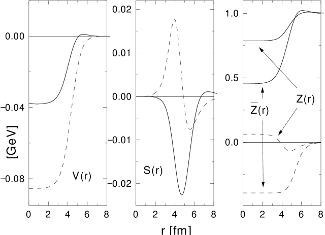
Fig. 3: The effective potential $V(r)$, the effective surface function $S(r)$ and the effective renormalization functions $Z(r),\,\bar{Z}(r)$ as introduced in (23) for the ${}^{58}_{28}$Ni K^- system. The solid and dashed lines represent the real and imaginary parts respectively.

We discuss the effect of the semi-classical optical potential (22) at hand of a $K^{-}$ bound at the ${}^{12}_{\;6}$C-core and ${}^{58}_{28}$Ni-core. We use the unfolded density profiles of [13, 3]:

$$\rho_{[^{12}_{\;6}C]}(r)=\rho_{0}\left(1+2.234\,\left(\frac{r}{1.516\,{\rm fm}}\right)^{2}\right)\exp\left(-\left(\frac{r}{1.516\,{\rm fm}}\right)^{2}\right)\;,$$

$$\rho_{[^{58}_{28}{\rm Ni}]}(r)=\rho_{0}\left(1+\exp\left(\frac{r-4.134\,{\rm fm}}{0.500\,{\rm fm}}\right)\right)^{-1}\;,$$ (24)

with $\rho_{0}$ determined by $4\,\pi\,\intop dr\,r^{2}\,\rho(r)=12$ for carbon and $4\,\pi\,\intop dr\,r^{2}\,\rho(r)=58$ for nickel. In Fig. 3 the effective potential $V(r)$, the effective surface function $S(r)$ and the renormalization functions $Z(r),\bar{Z}(r)$ defined in (23) are shown for the ${}^{58}_{28}$Ni density profile of (24). We point out that for the wave function and mass renormalization functions $Z(r)$ and $\bar{Z}(r)$ we find quite large deviations of about 50$\%$ from the asymptotic value 1. Also the function $S(r)$ shows sizeable strength close to the nucleus surface.

We introduce the nuclear level shift, $\mathchar 1\relax E$, in terms of the measured transition energy, $\mathchar 1\relax E_{\rm emp.}=\mathchar 1\relax E_{\rm e.m.}+\mathchar 1\relax E$, and the theoretical electromagnetic transition energy, $\mathchar 1\relax E_{\rm e.m.}$. For the ${}^{12}_{\;6}C\,K^{-}$ system we consider the 3d$\to$2p transition with $E_{\rm e.m.}$(2p) = 0.113763 MeV and $E_{\rm e.m.}$(3d) = 0.050458 MeV. For the ${}^{58}_{28}$Ni K^- system we consider the 5g$\to$4f transition with $E_{\rm e.m.}$(4f) = 0.641572 MeV and $E_{\rm e.m.}$(5g) = 0.409951 MeV. Here the Coulomb potential and the vacuum polarization potentials [12] are folded with the nucleus density profile (24). We use $m_{K^{-}}=493.677$ MeV and $1/\alpha=137.035989$. The empirical transition energy is $\mathchar 1\relax E_{\rm emp.}=62.73\pm 0.08$ keV with $\mathchar 0\relax=1.73\pm 0.15$ keV [15] for carbon and $\mathchar 1\relax E_{\rm emp.}=231.408\pm 0.052$ keV with $\mathchar 0\relax=1.230\pm 0.140$ keV for nickel. Note that the resulting empirical nuclear level shifts $\mathchar 1\relax E=-573\pm 80$ keV for carbon and $\mathchar 1\relax E=-213\pm 52$ keV for nickel differ slightly from the values given in [15, 23] and shown in Tab. 2. The reason for which is an old value for the kaon mass, a slightly different nucleus profile and the inclusion of further small correction terms.

	${}^{12}_{\;6}$C (3d$\to$2p)		${}^{58}_{28}$Ni (5g$\to$4f)
	$-\mathchar 1\relax E$ [eV]	$\mathchar 0\relax$ [eV]	$-\mathchar 1\relax E$ [eV]	$\mathchar 0\relax$ [eV]
$a_{KN}$	475	761	199	476
$a^{(\rm eff.)}_{KN}$	593	1362	143	932
$b_{\rm eff.}=0\;\;\&\;\;c_{\rm eff.}$ = 0	603	1022	248	627
$c_{\rm eff.}$ = 0	589	1109	278	759
full  theory	569	1098	233	701
experiment [15, 23]	590 $\pm$ 80	1730 $\pm$ 150	246 $\pm 52$	1230 $\pm 140$

Table 2: Results for the ${}^{12}_{\;6}$C K^- and ${}^{58}_{28}$Ni K^- systems. The first two rows show the results from the optical potential (1) with i) the empirical repulsive scattering length $a_{KN}=(-0.18+i\,0.67)$ fm and ii) the effective attractive scattering length $a^{(\rm eff.)}_{KN}=(0.63+i\,0.89)$ fm. The remaining rows show the result with the semi-classical optical potential (23) with iii) $b_{\rm eff.}=0=c_{\rm eff.}$, iv) with $c_{\rm eff.}=0$ and v) with $a_{\rm eff.},b_{\rm eff.}$ and $c_{\rm eff.}$ from Fig. 2.

In Tab. 2 we compare the results from the low-density optical potential (1) with the result of the semi-classical optical potential. The full semi-classical potential represents the empirical level shifts quantitatively but underestimates the empirical widths systematically. As can be seen from Tab. 2 the non-local effects increase the level widths by only a small amount towards the empirical values. The results obtained with the semi-classical potential differ significantly from the results obtained with phenomenological potential $V_{2}$ in (7) with an ad-hoc gradient ordering. We emphasize that the crucial assumption of our approach, namely that the results are insensitive to the precise form of the slope functions $b_{\rm eff.}(k_{F})$ and $c_{\rm eff.}(k_{F})$ in the extreme surface region $k_{F}<q\simeq 20$ MeV, which justifies the expansion (4), is fulfilled. The size of the level shifts and widths, using $b_{\rm eff.}(k_{F})$ and $c_{\rm eff.}(k_{F})$ functions modified according to (8), are affected by less than $3\%$ for the ${}^{12}_{\;6}$C K^- and ${}^{58}_{28}$Ni K^- systems. Note that this uncertainty is certainly not resolved by the accuracy of the available empirical level shifts and widths.

5 Summary

We summarize the findings of our work. The kaon self energy shows a rapid density, energy and momentum dependence in nuclear matter. This rich structure is a consequence of a proper many-body treatment of the $\mathchar 3\relax(1405)$ resonance structure in nuclear matter invalidating any mean field type approach to kaon propagation in nuclear matter at moderate densities. Thus non-local terms in the optical potential are large and quantitatively important. If included phenomenologically in the calculation of the kaonic atom spectra they cause substantial additional shifts of the binding energies and level widths. Since the kaon self energy must be obtained in a non-perturbative many-body approach it is not immediate as to which gradient ordering to choose. A phenomenological p-wave like ordering of gradient terms with the strength taken from the many-body calculation of [1, 17] leads to a satisfactory description of the kaonic atom level shifts. However, a proper microscopic description of $K^{-}$-atom data requires a careful derivation of the non-local part of the optical potential. Given the kaon self energy as evaluated for infinite nuclear matter, one can at most establish non-local terms where a gradient is acting on the kaon wave function. This follows in particular, because the low-momentum expansion of the self energy converges only for $q<k_{F}$ once the important Pauli blocking effects are considered. In this work we established that for such non-local effects the typical kaon momentum is indeed smaller than the typical Fermi momentum as probed in K-atoms. This justifies an expansion of the kaon self energy in small momenta. We reiterate that given only the kaon self energy of infinite nuclear matter any contribution considered for the optical potential which involves $\nabla^{2}\,\rho$ is not controlled and therefore must be dropped.

We derived the microscopic structure of the optical potential by means of the semiclassical expansion in the second part of this work systematically. At present this approach reproduces the empirical level shifts quantitatively but underestimates the empirical widths systematically. The microscopic optical potential leads to less pronounced non-local effects as compared to the phenomenological optical potential with p-wave like gradient ordering. Further improvements are conceivable. For instance the non-local effects involving $\nabla^{2}\rho$ should be studied and also p-wave interaction terms should be considered. Moreover, the kaonic atom data appear very sensitive to the precise microscopic interaction of the kaon-nucleon system. An improved microscopic input for the many-body calculation of the kaon self energy is desirable. This is supported by the recent chiral $SU(3)$ analysis of the kaon-nucleon scattering data which includes for the first time also p-wave effects systematically [20]. It is found that the subthreshold kaon-nucleon scattering amplitudes differ strongly from those of [10, 17] and that p-wave effects in the isospin one channel are strong. An evaluation of the many-body effects based on the improved chiral SU(3)-dynamics is in progress [24].

6 Appendix

In this appendix we derive the contribution from Pauli blocking to the in-medium kaon-nucleon scattering process and the kaon self energy. Pauli blocking induces a model independent term in the scattering amplitude $T^{(P.B.)}_{KN}(\omega+m_{N},\vec{q}\,)$ and self energy $\mathchar 5\relax^{(P.B.)}_{K}(\omega,\vec{q}\,)$ proportional to the squared s-wave scattering lengths:

$$T^{(P.B.)}_{KN}(\omega+m_{N},\vec{q}\,)=\pi\left(1+\kappa\right)\left(\left(a_{KN}^{(0)}\right)^{2}+3\,\left(a_{KN}^{(1)}\right)^{2}\right)I(\omega,\vec{q}\,)\;,$$

$$\mathchar 5\relax^{(P.B.)}_{K}(\omega,\vec{q})=-4\,\intop_{0}^{k_{F}}\frac{d^{3}p}{(2\pi)^{3}}\,T^{(P.B.)}_{KN}\big{(}\omega+m_{N}+p^{2}/(2\,m_{N}),\vec{p}+\vec{q}\,\big{)},$$

(25)

with $\kappa=m_{K}/m_{N}$ and

$$\!\!\!\!\!\!I(\omega,\vec{q}\,)=i\,p_{\rm cm}[\omega,\vec{q}\,]$$

$$-\intop_{0}^{k_{F}}\frac{d^{3}l}{(2\pi)^{3}}\,\frac{4\,\pi\,\big{(}1+\kappa\big{)}}{m_{K}^{2}+\mathchar 1\relax m_{K}^{2}-\omega^{2}+\big{(}1+\omega/m_{N}\big{)}\,\vec{l}\,^{2}-2\,\vec{l}\cdot\vec{q}+\vec{q}\,^{2}-i\,\epsilon},$$

$$\sqrt{(\omega+m_{N})^{2}-\vec{q}\,^{2}}=\sqrt{m_{N}^{2}+p^{2}_{\rm cm}[\omega,\vec{q}\,]}+\sqrt{m_{K}^{2}+\mathchar 1\relax m_{K}^{2}+p^{2}_{\rm cm}[\omega,\vec{q}\,]}.$$

(26)

Note that in the denominator of (26) we neglected relativistic correction terms of the form $(l^{2})^{n+1}/m_{N}^{2n}$ or $\omega\,(l^{2})^{n+1}/m_{N}^{2n+1}$ with $n\geq 1$ but kept the correction term $\omega/m_{N}$. The latter term is important since it renders the derivatives $\partial_{\omega}\mathchar 5\relax(m_{K},0)$ and $\partial_{q^{2}}\mathchar 5\relax(m_{K},0)$ finite and well defined at $\omega=m_{K}$ and $q^{2}=0$. We emphasize that the inclusion of the kaon mass modification $\mathchar 1\relax m_{K}^{2}\sim k_{F}^{3}$ as required in a self-consistent calculation [1] leads to a well defined behavior of $I(\omega,\vec{q}\,)$ close to $\omega\simeq m_{K}$ and $\vec{q}\simeq 0$. Similarly, as suggested in [25], one may include nuclear binding effects in $I(\omega,\vec{q}\,)$ by replacing $m_{N}\to m_{N}+\mathchar 1\relax m_{N}$ and $\omega\to\omega-\mathchar 1\relax m_{N}$ in the r.h.s of (26). This leads to identical results for the low-density limits $\partial_{\omega}\,T(m_{K}+m_{N},0)$ and $\partial_{q^{2}}\,T(m_{K}+m_{N},0)$ since only the combination $\mathchar 1\relax m_{K}+\mathchar 1\relax m_{N}$ is active at leading order and will cancel identically. It is straightforward to derive:

$$\frac{\partial}{\partial\,\omega}\,I(m_{K},0) = \frac{4}{\pi}\,\frac{m_{K}}{k_{F}}\,\frac{1}{1+\kappa}+{\mathcal{O}}\left(k_{F}^{0}\right)\;,$$

$$\frac{\partial}{\partial\,q^{2}}\,I(m_{K},0) = -\frac{2}{3\,\pi}\,\frac{1}{k_{F}}\,\frac{3\,\kappa-1}{(1+\kappa)^{2}}+{\mathcal{O}}\left(k_{F}^{0}\right)\;,$$ (27)

leading to our result (11). Note that the two terms in $I(\omega,\vec{q}\,)$ lead to contributions proportional to $1/\sqrt{\mathchar 1\relax m_{K}+\mathchar 1\relax m_{N}}$ in (27) which however cancel identically. Similarly one may expand

$$\intop_{0}^{k_{F}}\frac{d^{3}p}{(2\pi)^{3}}\,I\big{(}m_{K}+p^{2}/(2\,m_{N}),\vec{p}\,\big{)}=-\frac{k_{F}^{4}}{4\,\pi^{3}}\,\frac{1-\kappa^{2}+\kappa^{2}\,\ln\kappa^{2}}{(1-\kappa)^{2}\,(1+\kappa)}+{\mathcal{O}}\left(k_{F}^{5}\right)\;,$$

$$\frac{d}{d\,\omega}\Bigg{|}_{\omega=m_{K}}\,\intop_{0}^{k_{F}}\frac{d^{3}p}{(2\pi)^{3}}\,I\big{(}\omega+p^{2}/(2\,m_{N}),\vec{p}\,\big{)}=-\frac{k_{F}^{2}\,m_{K}}{2\,\pi^{3}}\,\frac{\ln|\kappa|}{1+\kappa}+{\mathcal{O}}\left(k_{F}^{3}\right)\;,$$

$$\frac{d}{d\,q^{2}}\Bigg{|}_{q^{2}=0}\,\intop_{0}^{k_{F}}\frac{d^{3}p}{(2\pi)^{3}}\,I\big{(}m_{K}+p^{2}/(2\,m_{N}),\vec{p}+\vec{q}\,\big{)}=\frac{k_{F}^{2}}{4\,\pi^{3}}\Bigg{(}\frac{7}{3}\,\frac{\ln|\kappa|}{1+\kappa}$$

$$\qquad\qquad\qquad\qquad+\frac{2}{3}\,\frac{1-\kappa^{2}+2\,\kappa^{2}\,\ln|\kappa|}{(1+\kappa)\,(1-\kappa)^{2}}\Bigg{)}+{\mathcal{O}}\left(k_{F}^{3}\right)\;,$$ (28)

and arrive at the low-density limit of $b_{\rm eff.}(0)$ and $c_{\rm eff.}(0)$ as given in (5). For completeness we included in (28) the integral leading to the $k_{F}^{4}$-term in the self energy given in [1]. Its limit for small $\kappa$ was derived in [26].

References

- [1] M. Lutz, Phys. Lett. B426, 12 (1998); M.F.M. Lutz, in Proc. Workshop on Astro-Hadron Physics, Seoul, Korea, October, 1997, nucl-th/980233.
- [2] E. Friedmann, A. Gal and C.J. Batty, Phys. Rep. 287, 385 (1997).
- [3] E. Friedman, A. Gal and C.J. Batty, Nucl. Phys. A579, 518 (1994).
- [4] M. Thies, Nucl. Phys. A298, 344 (1978).
- [5] W.A. Bardeen and E.W. Torigoe, Phys. Rev. C3, 1765 (1971).
- [6] M. Alberg, E.H. Henely and L. Wilets, Ann. Phys. 96, 43 (1976).
- [7] M. Mizoguchi, S. Hirenzaki and H. Toki, Nucl. Phys. A567, 893 (1994); Nucl. Phys. A585, 349c (1995).
- [8] R. Brockmann and W. Weise, Nucl. Phys. A308, 365 (1978).
- [9] E. Friedman, A. Gal, J. Mares and A. Cieply, Phys. Rev. C60, 024314 (1999).
- [10] T. Waas, N. Kaiser and W. Weise, Phys. Lett. B365, 12 (1996).
- [11] V. Koch, Phys. Lett. B337, 7 (1994); A. Ohnishi, Y. Nara and V. Koch, Phys. Rev. C56, 2767 (1997).
- [12] J. Blomqvist, Nucl. Phys. B48, 95 (1972).
- [13] H. de Vries, C.W. de Jaeger and C. Vries, Atomic Data and Nuclear Data 36, 495 (1987).
- [14] M. Krell and T.E.O. Ericson, Jour. Comp. Phys. 3, 202 (1968).
- [15] G. Backenstoss, A. Bamberger, I. Bergström, P. Bounin, T. Bunaciu, J. Egger, S. Hultberg, H. Koch, M. Krell, U. Lynen, H.G. Ritter, A. Schwitter, and R. Stearns, Phys. Lett. B38, 181 (1972).
- [16] P.D. Barnes, R.A. Eisenstein, W.C. Lam, J. Miller, R.B. Sutton, M. Eckhause, J.R. Kane, R.E. Welsh, D.A. Jenkins, R.J. Powers, A.R. Kunselman, R.P. Redwine and R.E. Segel, Nucl. Phys. A231, 477 (1974).
- [17] A. Ramos and E. Oset, Nucl. Phys. A671, 481 (2000); we thank A. Ramos for providing us with a table of the effective scattering length.
- [18] A. Baca, C. Garcia-Recio and J. Nieves, Nucl. Phys. A673, 335 (2000).
- [19] S. Hirenzaki, Y. Okumura, H. Toki, E. Oset and A. Ramos, Phys. Rev. C61, 055205 (2000); we thank A. Ramos for communicating the above paper prior to publication.
- [20] M.F.M. Lutz and E.E. Kolomeitsev, in Proceedings of the International Workshop XXVII on Gross Properties of Nuclei and Nuclear Excitations, Hirschegg, Austria, January, 2000.
- [21] L.S. Kisslinger Phys. Rev. 98, 761 (1955).
- [22] M. Brack, C. Guet and H.-B. Hakansson, Phys. Rep. 123, 276 (1985).
- [23] C. J. Batty, S.F. Biagi, M. Blecher, S.D. Hoath, R.A.J. Riddle, B.L. Roberts, J.D. Davies, G.J. Pyle, G.T.A. Squier, D.M. Asbury, A.S. Clough, Nucl. Phys. A329, 407 (1979).
- [24] C. Korpa and M. Lutz, in preparation.
- [25] C. Garcia-Recio, L.L. Salcedo and E. Oset, Phys. Rev. C39, 595 (1989).
- [26] C. Garcia-Recio, E. Oset, L.L. Salcedo, Phys. Rev. C37, 194 (1988).