Transport with three-particle interaction

Abstract

Starting from a point - like two - and three - particle interaction the kinetic equation is derived. While the drift term of the kinetic equation turns out to be determined by the known Skyrme mean field the collision integral appears in two - and three - particle parts. The cross section results from the same microscopic footing and is naturally density dependent due to the three - particle force. By this way no hybrid model for drift and cross section is needed for nuclear transport. Besides the mean field correlation energy the resulting equation of state has also a two - and three - particle correlation energy which are both calculated analytically for the ground state. These energies contribute to the equation of state and lead to an occurrence of a maximum at 3 times nuclear density in the total energy.

]

I Introduction

The equation of state of nuclear matter is known to saturate at the density of $n_{0}=0.16$fm^-3 with a binding energy of $-16$MeV. Refined two-particle calculations using Bruckner theory [1] and beyond [2] are not crossing the “Coester line” in that they lead to binding energies and/or densities above the saturation ones. Only density dependent Skyrme parameterizations originally introduced by Skyrme [3, 4], three-particle interactions [5, 6] or relativistic treatments [7] can reproduce the correct binding energy and saturation density of nuclear matter. The Skyrme parameterizations are derived from an effective three-particle interaction [8]. This leads to a nonlinear density dependence in the effective three - particle part which is responsible for saturation. The importance of three-particle collisions in nuclear matter transport has been demonstrated, e.g. in [9]. The density dependence deviating from that arising by three-body contact interaction has been introduced and compared with experiments in [10].

The relativistic approach on the other hand yields immediately the correct saturation with two - particle exchange interactions. This has been traced down to the nonlinear density dependence of scalar density and consequently nonlinear mean fields [11] which leads to a density contribution to the binding energy of $(n/n_{0})^{8/3}$. Higher order effects have been shown to lead to a $(n/n_{0})^{3.4}$ dependence, see [12] and citations therein. Therefore the physics of the saturation mechanism is certainly a nontrivial density dependence of the mean field. Though the Skyrme interaction has been overwhelmingly successful and the evidence of saturation by three-particle interaction [5, 6], it is puzzling that a transport theory with three-particle contact interaction has not been formulated. In this paper we will derive the corresponding kinetic equation using nonequilibrium Green’s function and we will show that the three-body interaction term leads to a $(n/n_{0})^{10/3}$ contribution to the binding energy.

The transport theory including three - particle interactions seems to be of wider interest e.g. in [13] it has been found that the three-body interactions have a measurable influence on thermodynamic properties of fluids in equilibrium. The description of nonequilibrium in nuclear matter is mostly based on the Boltzmann (BUU) equation which uses the Skyrme parameterization to determine the mean field and drift side of the kinetic equation. The collisional integral is then calculated with a cross section which arises from different theoretical impact. In addition one usually neglects the three-particle collision integral. These hybrid models have worked quite successfully despite their weak rigour in microscopic foundation.

In this paper the transport equation will be derived for two- and three - particle contact interactions. We will see that a natural density dependent mean field appears, in agreement with variational methods. Further we will obtain, on the same ground, density dependent cross sections. This has the advantage that we can derive a BUU equation which has the same microscopic impact on the drift and collisional side. Finally the three -particle collision integral appears naturally from this treatment. From balance equations we will derive the density dependent energy which gives the equation of state.

II Three - particle Kadanoff and Baym equation

We consider a Hamilton system with the Hamiltonian

$$H = \sum\limits_{i}a_{i}^{+}{\hbar^{2}\nabla^{2}\over 2m}a_{i}$$ (3)

$$+\frac{1}{2}\sum\limits_{ij}a_{i}^{+}a_{j}^{+}a_{i}a_{j}V_{2}(i,j)$$

$$+\frac{1}{6}\sum\limits_{ijk}a_{i}^{+}a_{j}^{+}a_{k}^{+}a_{i}a_{j}a_{k}V_{3}(i,j,k)$$

where $a_{i}^{+},a_{i}$ are creation and annihilation operators with cumulative variables $i=(x_{i},t_{i},...)$. We assume the potential is contact - like as

$$V_{2}(i,j) = t_{0}\delta(i-j)$$ (4)

$$V_{3}(i,j,k) = t_{3}\delta(i-j)\delta(i-k).$$ (5)

The Heisenberg equations of motion for the annihilation operators read

$$i\hbar\partial_{t_{1}}a_{1} = [a_{1},H]$$ (6)

$$= -{\hbar^{2}\nabla_{1}^{2}\over 2m}a_{1}+\sum\limits_{2}V(1,2)a_{2}^{+}a_{1}a_{2}$$ (8)

$$+\frac{1}{2}\sum\limits_{23}V(1,2,3)a_{2}^{+}a_{3}^{+}a_{1}a_{2}a_{3}.$$

From this we get the equation of motion for the causal Green function $G(1,2)=\frac{1}{i}<Ta_{1}^{+}a_{2}>$ with the time ordering $T$ and the average taken about the nonequilibrium density operator

$$(i\hbar\partial_{t_{1}}-{\hbar^{2}\nabla_{1}^{2}\over 2m})G(1,1^{\prime})=\delta(1-1^{\prime})$$ (9)

$$+\int d2V(1,2)G_{2}(1,2,1^{\prime},2^{+})$$ (10)

$$+\frac{1}{2}\int d2d3V(1,2,3)G_{3}(1,2,3,1^{\prime},2^{+},3^{+})$$ (11)

$$\equiv\delta(1-1^{\prime})-\int dx_{2}\Sigma_{HF}(x_{1},x_{2},t)G(x_{2},t,x_{1},t)$$ (12)

$$+\int d2(\Sigma(1,2)G(2,1^{\prime})-\Sigma^{>}(1,2)G^{<}(2,1^{\prime}))$$ (13)

where the $1^{+}$ denotes the space - time point $1=(x_{1},t_{1}+\epsilon)$ with a time infinitesimally larger than $1$. This equation is enclosed in the standard manner introducing the self energy $\Sigma$. We have split the mean field parts $\Sigma_{HF}$ including exchange and have introduced for the rest the self energy on the Keldysh contour. This is equivalent to the weakening of initial correlations. The correlation functions are $G^{<}(1,2)=<a_{2}^{+}a_{1}>$ and $G^{>}(1,2)=<a_{1}a_{2}^{+}>$ respectively and their equation of motion follows from (13) in the form of the known Kadanoff and Baym equation [14, 15]

$$i(G_{0}^{-1}G^{<}-G^{<}G_{0}^{-1})=\Sigma^{R}G^{<}-G^{<}\Sigma^{A}$$ (14)

where one takes advantage of the retarded and advanced functions $G^{R/A}=\mp i\theta[\pm(t_{1}-t_{2})](G^{>}\mp G^{<})$ and understands products as integration over inner variables.

FIG. 1.: The definition of self energy. We denote the two-particle interaction by long dashed lines and the three-particle interaction by short dashed line.

A Mean field parts

We first calculate the mean field parts. These parts come from the first order interaction diagrams of figure 1. To this end we use the two- and three- particle Green function in lowest order approximation seen in figure 2.

FIG. 2.: The lowest order expansion of Green functions. The statistical factor $g$ due to degeneracy in the system is indicated explicitly.

Introducing these diagrams into figure 1, one obtains for contact interaction (5)

$$\Sigma^{\rm HF}(1,1^{\prime})=\Biggl{[}{g\pm 1\over g}t_{0}n(1)+{(g\pm 1)(g\pm 2)\over 2g^{2}}t_{3}n(1)^{2}\Biggr{]}\delta(1-1^{\prime})$$ (15)

(16)

where we have used the fact that the density is $n(1)=G^{<}(1,1)/g$. Here and in the following we write the upper sign for Bosons and the lower sign for Fermions. The result (16) is the known Skyrme mean field expression in nuclear matter for $g=4$. It resembles an effective density dependent two-particle interaction arising from three-particle contact interaction. As a consistency check we see that for $g=2$ degenerated Fermionic system, like spin -1/2 Fermions, no three-body term appears. Pauli-blocking forbids two particles to meet at the same point with equal quantum numbers which one would have for three - particle contact interaction and degeneracy of $g=2$.

B Kinetic equation

For the kinetic equation we need as the lowest order approximation the next diagrams of figure 2 including one interaction line. While there are different expansion techniques at hand [16, 13] we will perform here a scheme as close as possible to the causal Green’s function including all exchanges which are presented in figure 2. This will give us the advantage that we can consider all diagrams which differ by exchange of outgoing lines as equal. To this aim we introduce the abbreviated symmetrized Green’s function with respect to incoming lines in figure 3.

FIG. 3.: The symmetrized three-body Green function with respect to incoming lines which are used in figure 5.

FIG. 4.: The introduced vertices. The three - and two - particle interaction potentials are the same as in figure1.

The expansion of the three -body Green’s function is given in figure 5. Besides the three -particle interaction potential we have to consider all possible single line interactions between two incoming lines. This is shortened by the introduction of the symmetrized Green function in figure 3 and the vertices of figure 4.

FIG. 5.: The first order expansion of the two - and three - particle Green’s functions with respect to interaction.

Since we can also have nontrivial combinations of two incoming lines and one free line for the three - body Green function we have introduced an auxiliary two - body Green function $G_{2}^{\rm s}$ which is defined in figure 5. Please note that the exchange of outgoing lines does not lead to distinguished diagrams. The two - particle Green function is then given by figure 5. Introducing now this expansion into the definition of self energy in figure 1 we obtain the 4 diagrams of figure 6. All other combinations lead either to disconnected diagrams or to equivalent ones by interchanging outgoing lines. Here the seemingly disconnected diagrams for $G_{3}^{1}$ in figure 5 lead together with the corresponding diagrams from $G_{2}^{1}$ to the vertex in front of $G^{s}_{2}$ of figure 6.

FIG. 6.: The self energy according to figure1 with the expansion of figure 5.

The enclosing diagram about the auxiliary Green function $G_{2}^{s}$ is given in figure 7. Please denote that here the seemingly disconnected diagrams of figure 5 vanish. We have used again the fact that the interchange of outgoing lines does not lead to distinguished diagrams.

FIG. 7.: The enclosing diagram of the auxiliary Green function $G_{2}^{s}$.

Inserting figure 7 in figure 6 we obtain the final result for the self energy in the Born approximation

$$\Sigma^{<}(1,1^{\prime})=(g\pm 1)\left[t_{0}^{2}\right.$$ (17)

$$+\left.(g\pm 2)\left(4t_{0}^{2}+6t_{3}^{2}{n(1)n(1^{\prime})\over g^{2}}+5t_{0}t_{3}({n(1)\over g}+{n(1^{\prime})\over g})\right)\right]$$ (18)

$$\times G^{<}(1,1^{\prime})^{2}G^{>}(1^{\prime}1)$$ (19)

$$+\frac{1}{2}(g\pm 1)(g\pm 2)t_{3}^{2}\,\,G^{<}(1,1^{\prime})^{3}G^{>}(1^{\prime}1)^{2}.$$ (20)

Note that all interactions vanish for the fermionic case $g=1$ since the Pauli-principle does not allow contact interaction in this case. For $g=2$ only the two - particle interactions survive for fermions as one expects from the Pauli principle. That the result is symmetric in the densities at the two time-space points needs no further comment.

From the self energy we can write down the Kadanoff and Baym equation (14) in closed form. If we employ standard gradient expansion and convert the equation (14) into an equation for the pole part of the Green’s function we obtain the final kinetic equation

$$\frac{\partial}{\partial t}f_{1}(t)+{p_{1}\over m}{\partial\over\partial r}f_{1}(t)-{\partial\over\partial r}\sigma^{\rm HF}(t){\partial\over\partial p_{1}}f_{1}(t)$$ (21)

$$= \frac{2}{\hbar^{2}}\int\frac{dp_{2}dp_{1}^{\prime}dp_{2}^{\prime}}{(2\pi\hbar)^{6}}T_{2}^{2}\delta(p_{1}+p_{2}-p_{1}^{\prime}-p_{2}^{\prime})$$ (22)

$$\times \int_{t_{0}}^{t}d\tau{\rm cos}\left[\frac{1}{\hbar}(E_{1}+E_{2}-E_{1}^{\prime}-E_{2}^{\prime})(t-\tau)\right]$$ (23)

$$\times \left\{f_{1}^{\prime}(\tau)f_{2}^{\prime}(\tau){\bar{f}_{1}}(\tau){\bar{f}_{2}}(\tau)-f_{1}(\tau)f_{2}(\tau){\bar{f}_{1}^{\prime}}(\tau){\bar{f}_{2}^{\prime}}(\tau)\right\}$$ (24)

$$+ \frac{2}{\hbar^{2}}\int\frac{dp_{2}dp_{3}dp_{1}^{\prime}dp_{2}^{\prime}dp_{3}^{\prime}}{(2\pi\hbar)^{12}}T_{3}^{2}\delta(p_{1}\!+\!p_{2}\!+\!p_{3}\!-\!p_{1}^{\prime}\!-\!p_{2}^{\prime}\!-\!p_{3}^{\prime})$$ (25)

$$\times \int_{t_{0}}^{t}d\tau{\rm cos}\left[(E_{1}+E_{2}+E_{3}-E_{1}^{\prime}-E_{2}^{\prime}-E_{3}^{\prime}){t-\tau\over\hbar}\right]$$ (27)

$$\times\left\{f_{1}^{\prime}(\tau)f_{2}^{\prime}(\tau)f_{3}^{\prime}(\tau){\bar{f}_{1}}(\tau){\bar{f}_{2}}(\tau){\bar{f}_{3}}(\tau)\right.$$

$$- \left.f_{1}(\tau)f_{2}(\tau)f_{3}(\tau){\bar{f}_{1}^{\prime}}(\tau){\bar{f}_{2}^{\prime}}(\tau){\bar{f}_{3}^{\prime}}(\tau)\right\}$$ (28)

with $\bar{f}=1-f$, and the particle dispersion $E=p^{2}/2m+\sigma^{\rm HF}$. The quasiparticle distribution functions are normalized to the density as $g\int{dp\over(2\pi\hbar)^{3}}f(p)=n$. For the sake of simplicity we have suppressed the notation of centre of mass space dependence. Neglecting the retardation in the distribution functions and taking $t_{0}\rightarrow\infty$ gives the standard Boltzmann two- and three- particle collision integrals.

The introduced two - and three- particle T-matrices are read off from (20) as first Born approximation

$$T_{2}^{2} = {g\pm 1\over g^{2}}\left[t_{0}^{2}\right.$$ (30)

$$+ \left.(g\pm 2)\left(4t_{0}^{2}+6t_{3}^{2}{n(1)n(1^{\prime})\over g^{2}}+5t_{0}t_{3}({n(1)\over g}+{n(1^{\prime})\over g})\right)\right]$$ (31)

$$T_{3}^{2} = \frac{1}{2}{g\pm 1\over g^{3}}(g\pm 2)t_{3}^{2}.$$ (32)

The reader is remind that we have generally to sum over collision partners and to average over the outgoing products. While the summation is already taken into account explicitly in the diagrammatic approach above we had to divide by $g^{2}$ and $g^{3}$ for the two- and three - particle outgoing collision partners respectively. An effective cross section can be defined in the usual way and read up to constants

$${d\sigma_{2}\over d\Omega} \sim T^{2}_{2}={3\over 16}\left[9{t_{0}^{2}}+\frac{3}{4}t_{3}^{2}n^{2}+5t_{0}t_{3}n\right]$$ (35)

$$={27\over 16}\left[(t_{0}+\frac{1}{6}t_{3}n)^{2}+\frac{2}{9}t_{3}n(t_{0}+\frac{1}{4}t_{3}n)\right]$$

$${d\sigma_{3}\over d\Omega} \sim T_{3}^{2}={3\over 64}t_{3}^{2}.$$ (36)

If one compares this with the effective two- particle cross section derived in [17] one sees that it differs by the last two terms of (36) proportional to $t_{3}$. This is due to the fact that the underlying three - particle process is taken into account explicitly here while in [17] an effective two - particle kinetic theory has been developed. Obviously we have to face a partial cancellation between three - and two - particle collisions. This will become explicit in the discussion of correlation energies. We will see that the two - and three - particle correlation energies indeed cancel partially concerning the $t_{3}$ terms.

The ratio of the effective cross sections are for the case of nuclear matter ($g=4$)

$${d\sigma_{2}\over d\sigma_{3}}={T_{2}^{2}\over T_{3}^{2}} = 4\left[9{t_{0}^{2}\over t_{3}^{2}}+\frac{3}{4}n^{2}+5{t_{0}\over t_{3}}n\right].$$ (37)

This could serve as the measure of relative importance of the corresponding collision processes, but we prefer to discuss this later in terms of dispersed energy by the two- and three- particle collision integrals since this includes also the Pauli blocking.

We would like to point out that we have fulfilled our task and have derived a kinetic equation where the drift as well as the collision integral follows from the same microscopic impact. The drift represents a Skyrme mean field and the collision side shows a two - and three - particle collision integral where the cross sections are calculated from the same parameters as the mean field.

III Balance equation

By multiplying the kinetic equation with $1,p$ and $E$, one obtains the balance for density $n$, momentum $u$ and energy ${\cal E}$. Since the collision integrals vanish for density and momentum balance we get the usual balance equations

$${\partial n\over\partial t}+{\partial\over\partial R}\int{dp\over(2\pi\hbar)^{3}}{\partial E\over\partial p}f=0$$ (38)

$${\partial u_{i}\over\partial t}+{\partial\over\partial R_{j}}\int{dp\over(2\pi\hbar)^{3}}(p_{i}{\partial E\over\partial p_{j}}f+{\cal E}\delta_{ij})=0$$ (39)

where the mean field energy of the system varies as

$$\delta{\cal E} = \int{dp\over(2\pi\hbar)^{3}}{\delta{\cal E}\over\delta f(p)}\delta f(p)$$ (40)

$$= \int{dp\over(2\pi\hbar)^{3}}E\delta f(p)$$ (41)

such that from (16) follows

$${\cal E}=<{k^{2}\over 2m}>+{g\pm 1\over 2g}t_{0}n^{2}+{(g\pm 1)(g\pm 2)\over 6g^{2}}t_{3}n^{3}.$$ (42)

With the help of this quantity the balance of energy density reads

$${\partial{\cal E}\over\partial t}+{\partial\over\partial R}\int{dp\over(2\pi\hbar)^{3}}E{\partial E\over\partial p}f=-{\partial\over\partial t}E_{\rm corr_{2}}(t)-{\partial\over\partial t}E_{\rm corr_{3}}(t)$$ (43)

with the two-particle correlation energy [18, 19]

$$E_{\rm corr_{2}}(t)$$ (45)

$$=-\frac{g}{\hbar}\int\limits_{t_{0}}^{t}d\tau\int\frac{dp_{1}dp_{2}dp_{1}^{\prime}dp_{2}^{\prime}}{(2\pi\hbar)^{9}}T_{2}^{2}\delta(p_{1}+p_{2}-p_{1}^{\prime}-p_{2}^{\prime})$$ (46)

$$\times\sin{\left[(E_{1}+E_{2}-E_{1}^{\prime}-E_{2}^{\prime}){t-\tau\over\hbar}\right]}f_{1}^{\prime}(\tau)f_{2}^{\prime}(\tau){\bar{f}_{1}}(\tau){\bar{f}_{2}}(\tau)$$ (47)

(48)

and the complete analogous expression for the three particle energy.

Please note that in the balance equations for the density and momentum no correlated density or correlated flux appears. This is due to the Born approximation. For more nontrivial approximations as e.g. the ladder summation these correlated observables appear [20, 21].

A Fit to nuclear matter ground state

As one can see, it is not enough to use the mean field parameterization to fit the equation of state as done in most approaches so far. Since the collision integral induces a two - particle and three - particle correlation energy we have to take this into account and have to refit the parameter $t_{0},t_{3}$ to the binding properties of nuclear matter. To illustrate this fact let us evaluate the fit without two - and three - particle correlation energy and therefore without collision integrals.

1 Hartree-Fock parameterization

Taking into account only Hartree-Fock mean field correlations (42) the ground state energy for nuclear matter reads

$${E\over A}={{\cal E}\over n}=\frac{3}{5}\epsilon_{f}+\frac{3}{8}t_{0}n+\frac{1}{16}t_{3}n^{2}.$$ (49)

Then the nuclear binding at $n_{0}=0.16$ fm^-3 with an energy of $E_{B}=-15.68$MeV is reproduced by the set

$$t_{0} = -{16\over 15n_{0}}(2\epsilon_{f}-5E_{B})=-1026.67{\rm MeV\,fm^{3}}$$ (50)

$$t_{3} = {16\over 5n_{0}^{2}}(\epsilon_{f}-5E_{B})=14625{\rm Mev\,fm^{6}}$$ (51)

which leads to a compressibility of

$$K=9n^{2}{\partial^{2}E/A\over\partial n^{2}}=\frac{9}{8}t_{3}n_{0}^{2}-\frac{6}{5}\epsilon_{f}=377{\rm MeV}.$$ (52)

2 Parameterization with two - and three - particle correlation energy

Now we consider the two - particle correlation energy. From (21) we obtain the total energy

$${\cal E}+E_{\rm corr_{2}}+E_{\rm corr_{3}}.$$ (53)

We want to calculate the long time limit which represents the equilibrium value. From the identity $\int\limits_{0}^{\infty}\sin{xt}dt={{\cal P}\over x}$ a principle value integration replaces the $sin$ term in (48)

$$E_{\rm corr_{2}}(\infty)=-g\int\frac{dp_{1}dp_{2}dp_{1}^{\prime}dp_{2}^{\prime}}{(2\pi\hbar)^{9}}T_{2}^{2}{{\cal P}\over E_{1}+E_{2}-E_{1}^{\prime}-E_{2}^{\prime}}$$ (54)

$$\times\delta(p_{1}+p_{2}-p_{1}^{\prime}-p_{2}^{\prime})f_{1}^{\prime}f_{2}^{\prime}{\bar{f}_{1}}{\bar{f}_{2}}.$$ (55)

For ground state Fermi distributions this expression can be integrated analytically [19] and we find from (55) the known Galitskii result for the two - particle ground state correlation energy [22]

$${E_{\rm corr_{2}}\over n} = 4\epsilon_{f}{2\log 2-11\over 35}({p_{f}mT_{2}\over 4\pi^{2}\hbar^{3}})^{2}$$ (56)

$$= -{5.7910^{-5}\over{\rm MeV\,fm}^{2}}n^{4/3}\left[9t_{0}^{2}+\frac{3}{4}t_{3}^{3}n^{2}+5t_{3}t_{0}n\right].$$ (57)

As pointed out in [23] we had to subtract here an infinite value, i.e. the term proportional to $f_{1}f_{2}$ in (55). This can be understood as renormalization of the contact potential and is formally hidden in $E_{\rm corr}(0)$ when time integrating equation (43). For finite range potentials we have an intrinsic cut-off due to range of interaction and such problems do not occur.

The correlational two - particle energy (57) is always negative for fermionic degeneracies $2<g<8$ and for bosonic degeneracy $g<4$. Since the leading density goes with $n^{10/3}$ it will dominate over the positive kinetic part which goes like $n^{2/3}$. We find that for densities around $3n_{0}$ the total energy has a maximum and starts to decrease continuously for higher densities. The maximal energy is changed towards higher values if we now include three - particle correlations since the latter remain positive and have the same leading density term as the two - particle correlational energy.

The three - particle part reads

$$E_{\rm corr_{3}}(\infty)=-g\int\frac{dp_{1}dp_{2}dp_{3}dp_{1}^{\prime}dp_{2}^{\prime}dp_{3}^{\prime}}{(2\pi\hbar)^{15}}T_{3}^{2}$$ (58)

$$\times \delta(p_{1}+p_{2}+p_{3}-p_{1}^{\prime}-p_{2}^{\prime}-p_{3}^{\prime})f_{1}^{\prime}f_{2}^{\prime}f_{3}^{\prime}{\bar{f}_{1}}{\bar{f}_{2}}{\bar{f}_{3}}$$ (59)

$$\times {{\cal P}\over E_{1}+E_{2}+E_{3}-E_{1}^{\prime}-E_{2}^{\prime}-E_{3}^{\prime}}.$$ (60)

The analytic result for the contact potential has not been given in the literature to our knowledge and reads

$${E_{\rm corr_{3}}\over n} = 4\epsilon_{f}{9013\over 2\cdot 9\cdot 25\cdot 77\cdot 13}({p_{f}^{4}mT_{3}\over 4\pi^{4}\hbar^{6}})^{2}$$ (61)

$$= {2.3710^{-6}\over{\rm MeV\,fm}^{2}}n^{10/3}t_{3}^{2}.$$ (62)

This three - particle correlation energy remains positive and has the same leading density behaviour of $n^{10/3}$ as the two - particle correlational energy. Since the pre-factor is smaller than the one for the two - particle correlational energy we obtain a maximum at 3 times nuclear density beyond which the two - particle part dominates and the total energy diverges negatively which would mean a collapse of the system. This clearly marks the limit of the Born approximation.

Taking now the correlational energy into account via (53) instead of only the Hartree Fock energy (49) we obtain a fit to the nuclear binding of

$$\tilde{t}_{0} = -745.71{\rm MeV\,fm^{3}}$$ (63)

$$\tilde{t}_{3} = 8272.8.{\rm MeV\,fm^{6}}$$ (64)

which leads to a compressibility of

$$\tilde{K}=351{\rm MeV}$$ (65)

which is somewhat lower than the mean field compressibility of (52). The comparison of the two equation of states with and without two - and three-particle correlations can be seen in figure 8. The inclusion of two - particle correlation energy leads to a maximum at 3 times nuclear density above which the system collapses. The complete result including three particle correlational energy leads to a higher reachable maximum.

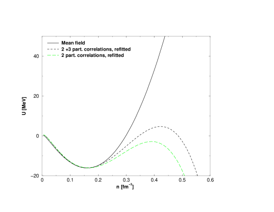
FIG. 8.: The equation of state due to mean field compared with the equation of state including two - and three - particle collisions in Born approximation.

B Importance of three particle collisions

We have seen that the three - particle contact interaction induces in a natural way a density dependence of the two - particle cross section. Additionally we have obtained an explicit three - particle collision integral on the same microscopic footing. We want now to answer the question how important the three - particle collisions are. Therefore we use as a measure the ratio of the two- and three - particle ground state correlation energies, (57) and (62), since this gives the measure of how much energy is maximally dispersed by the corresponding integrals. We obtain

$$\left|{E_{2}\over E_{3}}\right| = {2^{5}\cdot 5\cdot 11\cdot 13\over 9013}(11-2\log{2})$$ (66)

$$\times \left[9{t_{0}^{2}\over n^{2}t_{3}^{2}}+\frac{3}{4}+5{t_{0}\over t_{3}n}\right].$$ (67)

This ratio is decreasing until it reaches the density

$$n_{\rm min}=-{18t_{0}\over 5t_{3}}=0.32{\rm fm}^{-3}$$ (68)

where the ratio has the minimum

$$\left|{E_{2}\over E_{3}}\right|_{\rm min}=1.4.$$ (69)

For higher densities the constant value

$$\left|{E_{2}\over E_{3}}\right|_{\infty}=18.3$$ (70)

is approached.

I other words this means that the importance of three particle collisions increase with increasing density up to twice the nuclear density where the correlational energies are nearly equal. For higher densities we have 18 times larger two -particle correlational energies than three -particle ones. At nuclear saturation density this ratio is

$$\left|{E_{2}\over E_{3}}\right|_{n_{0}}=19.2$$ (71)

indicating that the three -particle collisions become important between nuclear density and twice the nuclear density while it can be neglected in the other cases.

IV Conclusions

For a microscopic two - and three - particle contact interaction consisting of two parameters the Kadanoff and Baym equation of motion is derived. From this a Boltzmann kinetic equation is obtained with drift which turns out to be the known Skyrme Hartree Fock expression while the collision side consists of two - and three - particle collision integrals. The two - particle collision integral contains an explicit density - dependent cross section arising from the three - particle contact interaction. By this way both the drift side as well as collision side is derived from the same microscopic footing and no hybrid assumptions about separate density dependent mean field and cross section is needed.

The correlational energy for the three- and the two - particle part are calculated analytically. Due to the density dependent two - particle collision integral both correlational energies have the same leading power of $(n/n_{0})^{10/3}4$ in density which shows that both contributions are of the same importance if three - particle interaction has to be considered. This is clearly motivated by the saturation point where non - relativistic two - particle approaches fail to overcome the “Coester line”.

We find that there is a maximum in the energy at 3 times nuclear density if two - and three particle correlational energies are included. Beyond this density the Born approximation fails at least in that the system collapses towards diverging negative energy.

While the two - particle collision cross section has a natural density dependence due to three - particle contact interaction it turns out that the explicit three particle collision integral can be neglected as long as one is below nuclear density. Around twice nuclear density the three particle collision integral has the same importance as the two - particle one since it disperses the same amount of energy. For higher densities the three - particle collision integral is again negligible.

I would like to thank H.S. Köhler and P. Lipavsky for numerous discussions and the LPC for a friendly and hospitable atmosphere. P. Chocian is thanked for reading the manuscript.

REFERENCES

- [1] H. S. Köhler, Phys. Rep. 18, 217 (1975).
- [2] M. Hjorth-Jensen, H. Muether, A. Polls, and E. Osnes, J. Phys. G 22, 321 (1996).
- [3] T. H. R. Skyrme, Phil. Mag. 1, 1043 (1956).
- [4] T. H. R. Skyrme, Nucl. Phys. 9, 615 (1959).
- [5] J. Carlson, V. Pandharipande, and R. Wiringa, Nucl. Phys. A 401, 59 (1983).
- [6] A. Jackson, M. Rho, and E. Krotscheck, Nucl. Phys. A 407, 495 (1983).
- [7] T. Gross-Boelting, C. Fuchs, and A. Faessler, Nucl. Phys. A 648, 105 (1999).
- [8] D. Vautherin and D. M. Brink, Phys. Rev. C 5, 626 (1972).
- [9] A. Bonasera, F. Gulminelli, and J. Molitoris, Phys. Rep. 243, 1 (1994).
- [10] H. S. Köhler, Nucl. Phys. A 258, 301 (1976).
- [11] A. Bouyssy, J. F. Mathiot, and N. V. Giai, Phys. Rev. C 36, 380 (1987).
- [12] G. E. Brown, W. Weise, G. Baym, and J. Speth, Comm. Nucl. Part. Phys. 17, 39 (1987).
- [13] S. Sinha, J. Ram, and Y. Singh, Physica A 133, 247 (1985).
- [14] L. P. Kadanoff and G. Baym, Quantum Statistical Mechanics (Benjamin, New York, 1962).
- [15] P. Lipavský, V. Špička, and B. Velický, Phys. Rev. B 34, 6933 (1986).
- [16] P. Danielewicz, Ann. Phys. (NY) 197, 154 (1990).
- [17] S. Ayik, O. Yilmaz, A. Golkalp, and P. Schuck, Phys. Rev. C 58, 1594 (1998).
- [18] K. Morawetz, Phys. Lett. A 199, 241 (1995).
- [19] K. Morawetz and H. Köhler, Eur. Phys. J. A 4, 291 (1999).
- [20] V. Špička, P. Lipavský, and K. Morawetz, Phys. Lett. A 240, 160 (1998).
- [21] P. Lipavský, K. Morawetz, and V. Špička, (1999), book sub. to Annales de Physique, K. Morawetz, Habilitation University Rostock 1998.
- [22] D. Pines and P. Nozieres, The Theory of Quantum Liquids (Benjamin, New York, 1966), Vol. 1.
- [23] E. Lifschitz and L. P. Pitaevsky, in Physical Kinetics, edited by E. Lifschitz (Akademie Verlag, Berlin, 1981).